Active conductivity of plane two-barrier resonance tunnel structure as operating element of quantum cascade laser or detector

Abstract

Within the model of rectangular potentials and different effective masses of electrons in different elements of plane two-barrier resonance tunnel structure there is developed a theory of spectral parameters of quasi-stationary states and active conductivity for the case of mono-energetic electronic current interacting with electromagnetic field. It is shown that the two-barrier resonance tunnel structure can be utilized as a separate or active element of quantum cascade laser or detector. For the experimentally studied In_0.53Ga_0.47As/In_0.52Al_0.48As nano-system it is established that the two-barrier resonance tunnel structure, in detector and laser regimes, optimally operates (with the biggest conductivity at the smallest exciting current) at the quantum transitions between the lowest quasi-stationary states.

resonance tunnel structure, conductivity, quantum laser, quantum detector 73.21.Fg, 73.90.+f, 72.30.+q, 73.63.Hs

Abstract

У моделi прямокутних потенцiалiв i рiзних ефективних мас електрона в рiзних елементах плоскої двобар’єрної резонансно-тунельної структури (ДБРТС) розвинута квантово-механiчна теорiя спектральних параметрiв квазiстацiонарних станiв i провiдностi цiєї системи для випадку моноенергетичного пучка електронiв, якi взаємодiють з електромагнiтним полем. Показано, що нано-ДБРТС може слугувати окремим елементом або активним елементом каскадного лазера чи детектора. На прикладi експериментально дослiджуваної наносистеми In_0.53Ga_0.47As/In_0.52Al_0.48As показано, що у детекторному i лазерному режимах робота ДБРТС є оптимальною (з найбiльшою провiднiстю при найменшому струмi збудження), коли вона працює на квантових переходах мiж найнижчими квазiстацiонарними станами. резонансно-тунельна структура, провiднiсть, квантовий лазер, квантовий детектор

1 Introduction

During the last decades, after the creation of the first nano-lasers by Faist and Capasso [1, 2] working at the transitions between electronic levels of size-quantization, the evident success was achieved in the improvement of quantum cascade lasers (QCLs) [3, 4, 5, 6] and quantum cascade detectors (QCDs) [7, 8, 9, 10] with various geometric design. These devices operate effectively in the actual terahertz range of electromagnetic waves with the frequencies getting into the known atmosphere transparency windows. Thus, the QCLs and QCDs are constantly in the field of researchers’ vision.

The main purpose of investigations is to optimize the parameters of nano-devices which is actually a hard task due to the absence of a consequent and complete theory of physical processes in open nano-systems. As far as the active working element in experimentally produced QCL or QCD were the open resonance tunnel structures (RTS), with different number of barriers and wells, the main theoretical attention was paid to the study of static and dynamic conductivities in such nano-systems because they determine the main QCL or QCD parameters, such as region and width of operating frequency range, radiation intensity, exciting current and so on.

The theory of dynamic conductivity [11, 12, 13, 14, 15, 16, 17] of electrons in open RTS, as separate active element of QCL working in ballistic regime, is developed within the analytic solution of complete Schrodinger equation using the simplified model of electron constant effective mass in all parts of nano-system and $\delta$-like approximation of rectangular potential barriers. In the cited and other papers, based on the simplified model of RTS, important results were obtained explaining the general properties of conductivity in open systems, but due to the rather rough approximating models, as it was established in reference [18], the obtained magnitudes of resonance energies and width of electron quasi-stationary states in RTS (essentially determining the conductivity magnitude) were manifestly overestimated compared to the more realistic model of rectangular potentials. Therefore, in the approximated model, the problem of the optimization of QCL, QCD or the operation of separate elements was not observed at all.

In the paper, using the model of rectangular potential wells and barriers and considering different electron effective masses in different parts, there is developed a theory of active conductivity of open plane two-barrier RTS as separate nano-detector or nano-laser. For the nano-system with In_0.53Ga_0.47As wells and In_0.52Al_0.48As barriers the best geometric design of two-barrier RTS is established providing its optimal work as an active element of nano-detector or nano-laser, i.e., providing the maximal active conductivity through the RTS at the minimal life times of electrons in the operating quasi-stationary states (QSSs). Besides, it is shown that contrary to the laser where the radiation transitions between two lowest electron QSS-s are not always optimal, the energy of mono-energetic electron beam falling at two-barrier RTS should correspond to the energy of the lowest QSS (from which the quantum transitions into the second resonance electron state occur with the absorption of electromagnetic energy) for the detector to operate effectively.

2 Active conductivity of two-barrier RTS

In Cartesian coordinate system, the open two-barrier RTS is observed with geometric parameters shown in figure 1. The small differences of lattice constants of RTS barriers and wells make it possible to study the nano-system within the models of effective masses and rectangular potentials

$$m(z)={\left\{{{\begin{array}[]{*{20}c}{m_{0}}\,,\hfill\\ {m_{1}}\,,\hfill\\ \end{array}}}\right.}\qquad U(z)={\left\{{{\begin{array}[]{*{20}c}{0,\qquad reg.\ 0,\,2,\,4,\hfill}\\ {U,\qquad reg.\,\,1,\,3.\hfill}\\ \end{array}}}\right.}$$ (1)

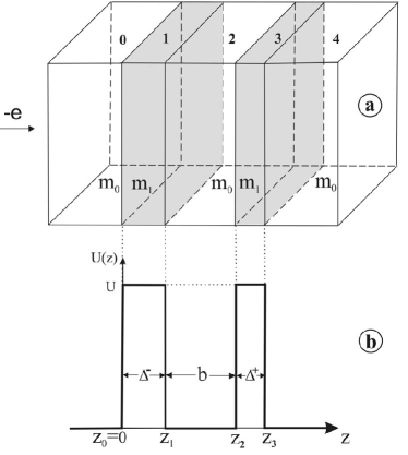
Figure 1: Geometric (a) and potential energy (b) schemes of two-barrier resonance tunnel structure.

The electronic beam moving in the direction perpendicular to the two-barrier RTS plane, impinges on it from the left hand side. The electrons with energy $(E)$ and concentration $(n_{0})$ are assumed to be uncoupled. In order to obtain the conductivity of a nano-system, determined by the density of current flowing through it, according to the quantum mechanics, one has to find the wave function of the electron dependent on time, interacting with the electromagnetic field periodic in time.

In the problem under study, the movement of electrons is observed as one-dimensional ($k_{||}=0$). Consequently, $\Psi(z,t)$ wave function satisfies the complete Schrodinger equation

$$\ri\hbar{\frac{{\partial\Psi(z,t)}}{{\partial t}}}=\left[{H+H(z,t)}\right]\Psi(z,t),$$ (2)

where

$$H=-{\frac{{\hbar^{2}}}{{2}}}{\frac{{\partial}}{{\partial z}}}{\frac{{1}}{{m\left({z}\right)}}}{\frac{{\partial}}{{\partial z}}}+U(z)$$ (3)

is the electron Hamiltonian in stationary case,

$$H(z,t)=-e\epsilon{\rm}\left\{{z\left[{\theta\left({z}\right)-\theta\left({z-z_{3}}\right)}\right]+z_{3}}{\theta\left({z-z_{3}}\right)}\right\}\left({\re^{\ri\omega t}+\re^{-\ri\omega t}}\right).$$ (4)

The Hamiltonian of an electron interacts with time varying electromagnetic field with frequency ($\omega$) and amplitude of electric field intensity ($\epsilon$).

The solution of equation (2) in the approximation of small signal [11, 12, 13, 14, 15, 16, 17] is written as follows:

$$\Psi\left({z,t}\right)=\Psi_{0}\left({z}\right)\re^{-\ri\omega_{0}t}+\Psi_{1}\left({z,t}\right),\qquad(\omega_{0}=E/\hbar)$$ (5)

where $\Psi_{0}(z)$ function is the solution of stationary Schrodinger equation

$$H\Psi_{0}(z)=E\Psi_{0}(z).$$ (6)

The first order correction in one-mode approximation is found as

$$\Psi_{1}\left({z,t}\right)=\Psi_{+1}\left({z}\right)\re^{-\ri\left({\omega_{0}+\omega}\right)t}+\Psi_{-1}\left({z}\right)\re^{-\ri\left({\omega_{0}-\omega}\right)t}.$$ (7)

Preserving the magnitudes of the first smallness order and taking into account formulas (5), (6), (2), the equation is obtained for the both parts $\Psi_{\pm 1}(z)$ of function $\Psi_{1}(z,t)$

$$\left({-{\frac{{\hbar^{2}}}{{2}}}{\frac{{\partial}}{{\partial z}}}{\frac{{1}}{{m\left({z}\right)}}}{\frac{{\partial}}{{\partial z}}}+U(z)-\hbar\left({\omega_{0}\pm\omega}\right)}\right)\Psi_{\pm 1}\left({z}\right)+H\left({z}\right)\Psi_{0}\left({z}\right)=0,$$ (8)

where

$$H(z)=-e\epsilon\left\{{z\left[{\theta\left({z}\right)-\theta\left({z-z_{3}}\right)}\right]+z_{3}\theta\left({z-z_{3}}\right)}\right\}.$$

The solution of stationary Schrodinger problem, equation (6) is written as

$$\Psi_{0}(z) = \Psi_{0}^{(0)}(z)\theta(-z)+\sum\limits_{p=1}^{3}{\Psi_{0}^{(p)}(z){\left[{\theta(z-z_{p-1})-\theta(z-z_{p})}\right]}}+\Psi_{0}^{(4)}(z)\theta(z-z_{3})$$ (9)

$$= \left({\re^{\ri k^{(0)}z}+B^{(0)}\re^{-\ri k^{(0)}z}}\right){\rm}\theta(-z)+A^{(4)}\re^{\ri k^{(4)}z}\theta(z-z_{3})$$

$${}+{\sum\limits_{p=1}^{3}{\left({A^{(p)}\re^{\ri k^{(p)}z}+B^{(p)}\re^{-\ri k^{(p)}z}}\right){\left[{\theta(z-z_{p-1})-\theta(z-z_{p})}\right]}}},$$

where

$$k^{(0)}=k^{(2)}=k^{(4)}=k=\hbar^{-1}\sqrt{2m_{0}E}\,,\qquad k^{(1)}=k^{(3)}=\hbar^{-1}\sqrt{2m_{1}(E-U)}\,,$$

$$z_{0}=0,\qquad z_{1}=\Delta_{1}^{-},\qquad z_{2}=b+\Delta_{1}^{-},\qquad z_{3}=b+\Delta,\qquad\Delta=\Delta_{1}^{-}+\Delta_{1}^{+}.$$

The unknown coefficients $B^{(0)}$, $A^{(4)}$, $A^{(p)}$, $B^{(p)}$ $(p=1,\ 2,\ 3)$ are fixed by the conditions of wave functions and their densities of currents continuity at all nano-system interfaces

$$\Psi_{0}^{(p)}(z_{p})=\Psi_{0}^{(p+1)}(z_{p}),\qquad{\frac{{1}}{{m_{0(1)}}}}{\left.{{\frac{{\rd\Psi_{0}^{(p)}}}{{\rd z}}}}\right|}_{z=z_{p}}={\frac{{1}}{{m_{1(0)}}}}{\left.{{\frac{{\rd\Psi_{0}^{(p+1)}(z)}}{{\rd z}}}}\right|}_{z=z_{p}}\qquad(p=0,\ 1,\ 2,\ 3)$$ (10)

as well as because the nano-system is an open one, from the normalizing condition for the wave functions (at fixed $k_{||}=0$)

$${\int\limits_{-\infty}^{\infty}{\Psi_{0}^{*}({k}^{\prime}z)\Psi_{0}(kz)}}{\rm}\rd z=\delta(k-{k}^{\prime}).$$ (11)

The obtained wave function $\Psi_{0}$ defines the density of electronic current and, thus, the permeability coefficient of the system as function of energy. It is well known [18], that the permeability coefficient in the vicinity of their maxima is of a quasi-Lorentz shape. Consequently, the position of maximum in the energy scale defines the resonance energy ($E_{n}$) and the width of Lorentz curve at half of its height fixes the resonance width ($\Gamma_{n}$) of the corresponding QSS.

The solutions of inhomogeneous equations (8) are the super-positions of functions

$$\Psi_{\pm 1}\left({z}\right)=\Psi_{\pm}\left({z}\right)+\Phi_{\pm}\left({z}\right),$$ (12)

where $\Psi_{\pm}\left({z}\right)$ are the solutions of homogeneous and $\Phi_{\pm}\left({z}\right)$ are solutions of inhomogeneous equations (8).

The solutions of homogeneous equations (8) are found as

$$\Psi_{\pm}(z) = \Psi_{\pm}^{(0)}(z)\theta(-z)+{\sum\limits_{p=1}^{3}{\Psi_{\pm}^{(p)}(z){\left[{\theta(z-z_{p-1})-\theta(z-z_{p})}\right]}}}+\Psi_{\pm}^{(4)}(z)\theta(z-z_{3})$$ (13)

$$= B_{\pm}^{(0)}\re^{-\ri k_{\pm}^{(0)}z}\theta(-z)+A_{\pm}^{(4)}\re^{\ri k_{\pm}^{(4)}\left({z-z_{3}}\right)}\theta(z-z_{3})$$

$${}+{\sum\limits_{p=1}^{3}{{\left[{B_{\pm}^{(p)}\re^{-\ri k_{\pm}^{(p)}(z-z_{p-1})}+A_{\pm}^{(p)}\re^{\ri k_{\pm}^{(p)}(z-z_{p-1})}}\right]}}}{\left[{\theta(z-z_{p-1})-\theta(z-z_{p})}\right]},$$

where

$$k_{\pm}^{(0)}=k_{\pm}^{(2)}=k_{\pm}^{(4)}=\hbar^{-1}\sqrt{2m_{0}(E\pm\hbar\omega)}\,,\qquad k_{\pm}^{(1)}=k_{\pm}^{(3)}=\hbar^{-1}\sqrt{2m_{1}\left[{(E-U)\pm\hbar\omega}\right]}\,.$$ (14)

Exact partial solutions of equations (8) are known

$$\Phi_{\pm}(z) = {\sum\limits_{p=1}^{3}{{\left[{\mp{\displaystyle\frac{{e\epsilon}}{{\hbar\omega}}}z\,\Psi_{0}^{(p)}\left({z}\right)+{\displaystyle\frac{{e\epsilon}}{{m_{p}\omega^{2}}}}{\displaystyle\frac{{\rd\Psi_{0}^{(p)}\left({z}\right)}}{{\rd z}}}}\right]}}}{\left[{\theta(z-z_{p-1})-\theta(z-z_{p})}\right]}$$ (15)

$${}\mp\displaystyle{\frac{{e\epsilon}}{{\hbar\omega}}}z_{3}\Psi_{0}^{(4)}\left({z_{3}}\right)\theta(z-z_{3}){\rm}.$$

Thus, the general solutions of these equations can be written as

$$\Psi_{\pm 1}\left({z}\right)=\Psi_{\pm 1}^{(0)}\left({z}\right){\rm}\theta(-z)+{\sum\limits_{p=1}^{3}{\Psi_{\pm 1}^{(p)}\left({z}\right){\rm}{\left[{\theta(z-z_{p-1})-\theta(z-z_{p})}\right]}}}+\Psi_{\pm 1}^{(4)}\left({z}\right){\rm}\theta(z-z_{3}).$$ (16)

The conditions of the equations of wave functions (16) and the respective continuity of currents at all interfaces of nano-systems

$$\Psi_{\pm 1}^{(p)}\left({z_{p}}\right)=\Psi_{\pm 1}^{(p+1)}\left({z_{p}}\right),\qquad{\left.{{\frac{{\rd\Psi_{\pm 1}^{(p)}\left({z}\right)}}{{m_{0(1)}\rd z}}}}\right|}_{z=z_{p}}={\left.{{\frac{{\rd\Psi_{\pm 1}^{(p+1)}\left({z}\right)}}{{m_{1(0)}\rd z}}}}\right|}_{z=z_{p}}\qquad(p=0,\ 1,\ 2,\ 3)$$ (17)

lead to the system of eight inhomogeneous equations determining all eight unknown coefficients $B_{\pm}^{(0)}$, $A_{\pm}^{(4)}$, $B_{\pm}^{(p)}$, $A_{\pm}^{(p)}$ $(p=1,\ 2,\ 3)$. Thus, now $\Psi_{\pm}(z)$ functions, the first order correction – $\Psi_{1}(z,t)$ and, consequently, the whole $\Psi(z,t)$ wave function are completely defined.

According to the quantum mechanics, the density of current of uncoupling electrons with concentration $n_{{\rm 0}}$ is given by the formula

$$j(z,t)={\frac{{\ri e\hbar{\rm}n_{0}}}{{2m(z)}}}{\left[{\Psi(z,t){\frac{{\partial}}{{\partial z}}}\Psi^{\ast}(z,t)-\Psi^{\ast}(z,t){\frac{{\partial}}{{\partial z}}}\Psi(z,t)}\right]}.$$ (18)

Taking into account the small sizes of two-barrier RTS compared to the electromagnetic wavelength, in quasi-classic approximation [11, 12, 13, 14, 15, 16, 17] the calculation of the guided current density is performed, determining the real part of nano-system conductivity

$$\begin{array}[]{c}\sigma(\omega)=\sigma^{+}(\omega)+\sigma^{-}(\omega)={\displaystyle\frac{{\hbar^{2}\omega{\rm}n_{0}}}{{2z_{3}m_{0}\epsilon^{2}}}}{\left[{k_{+}\left({{\left|{B_{+}^{(0)}}\right|}^{2}+{\left|{A_{+}^{(4)}}\right|}^{2}}\right)-k_{-}\left({{\left|{B_{-}^{(0)}}\right|}^{2}+{\left|{A_{-}^{(4)}}\right|}^{2}}\right)}\right]}.\end{array}$$ (19)

Here $\sigma^{+}(\omega)$, $\sigma^{-}(\omega)$ are the components of conductivity throughout the nano-system and in the opposite direction, respectively, caused by the electronic currents from the nano-system after the interaction with electromagnetic field therein.

3 Discussion of the results

The operating characteristics of a separate nano-laser, nano-detector or quantum cascade nano-devices at their base are determined by the properties of active conductivity, depending on spectral parameters (resonance energies and widths) of electron QSSs. The latter characteristics, in turn, are defined by material and geometric parameters of a nano-system. Thus, one has to study, first of all, the spectral parameters of electron QSSs for further analyzing and understanding the main properties of the active conductivity. For example, the paper studies the widely experimentally investigated [1, 2, 3, 7, 8, 9, 10] plane two-barrier RTS (figure 1), consisting of In_0.53Ga_0.47As wells ($m_{0}=0.046~{}m_{e}$) and In_0.52Al_0.48As barriers ($m_{1}=0.089~{}m_{e}$). The difference of electron potential energy between the barrier and the well is $U=516$ meV. This structure well satisfies the developed theory conditions due to the close magnitudes of lattice constants ($a_{0}=0.5867$ nm, $a_{1}=0.5868$ nm), wells ($\varepsilon_{0}=14.2$) and barriers ($\varepsilon_{1}=12.7$) dielectric constants.

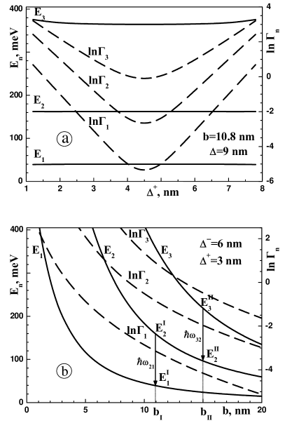
Figure 2: Dependencies of resonance energies $E_{n}$ and logarithms of resonance widths $\ln\Gamma_{n}$ : (a) on output barrier width $\Delta^{+}$ at $\Delta=9$ nm and (b) on well width $b$.

In figure 2 there are shown the resonance energies ($E_{n}$) and logarithms of resonance widths ($\ln\Gamma_{n}$ , in units $\Gamma_{0}=1$ meV) of the three lowest electron QSSs depending on geometric parameters of two-barrier RTS: i.e., on the width of the output barrier $\Delta^{+}$ (figure 2 (a)) at constant well width $b=10.8$ nm with sum barriers width $\Delta=\Delta^{-}+\Delta^{+}=9$ nm; potential well width $b$ (figure 2 (b)) at the fixed barriers widths $\Delta^{-}=6$ nm, $\Delta^{+}=3$ nm. The resonance energy ($E_{n}$) of electron n-th QSS is fixed by the position of maximum of n-th peak of permeability coefficient and the resonance width ($\Gamma_{n}$) – as the width of the same peak at the half of its height in energy scale.

From figure 2 it is clear that the change of both widths of barriers ($\Delta^{-}$, $\Delta^{+}$) almost does not change the spectrum of resonance energies ($E_{n}$), as square function of quantum number $n$. That is: $E_{n}=E_{1}n^{2}$, like the spectrum of quasi-particle in infinitely deep potential well. Here $E_{1}$ is the resonance energy of the first electron QSS in two-barrier RTS (fixed, as it was mentioned above, by the position of the first maximum of permeability coefficient in energy scale).

Contrary to the resonance energies ($E_{n}$), the magnitudes of resonance widths ($\Gamma_{n}$) essentially depend on the ratio between the barrier widths. It is clear (figure 2 (a)) that the increasing width of the output barrier ($\Delta^{+}$) and the respective decreasing width of the input barrier ($\Delta^{-}=\Delta-\Delta^{+}$) causes a linear decrease of all $\ln\Gamma_{n}$ , approaching the minima magnitudes at $\Delta^{+}=\Delta^{-}=4.5$ nm. At further $\Delta^{+}$ increase, the magnitudes of $\ln\Gamma_{n}$ linearly increase. Such a behavior of the width of electron QSSs ($\Gamma_{n}$) in $0<\Delta^{\pm}<\Delta/2$ range can be described by the typical, for the quantum-barrier systems, dependence: $\Gamma_{n}=\Gamma_{n}^{0}\exp(-\gamma_{n}\Delta^{\pm})$, where $\Gamma_{n}^{0}$ is the width of $n$-th virtual QSS, existing at $\Delta^{\pm}=0$, $\Delta^{\mp}=\Delta\neq 0$, $b\neq 0$. The magnitudes $\gamma_{n}$ characterize the speed of resonance widths decrease when the barriers width ($\Delta^{\pm}$) increases.

The dependence of electron QSSs spectral parameters ($E_{n}$ , $\Gamma_{n}$) on the well width ($b$) is shown in figure 2 (b). In the figure one can see that for the increasing well width, the resonance energies ($E_{n}$) and logarithms of resonance widths ($\ln\Gamma_{n}$) shift into the region of smaller energies. Herein, $E_{n}\sim b^{-3/2}$, contrary to the energy spectrum in infinitely deep potential well, where $E_{n}\sim b^{-2}$. The decreasing character of resonance widths is caused by a decrease of resonance energies which is equivalent to the increase of effective potential barriers above them.

The numerical calculations prove that the established properties of spectral parameters ($E_{n}$ , $\Gamma_{n}$) of electron QSSs are equitable at any magnitudes of two-barrier RTS geometric parameters ($b$, $\Delta^{\pm}$, $\Delta$). Further, the active conductivity of nano-system is studied as a function of energy ($E$) of mono-energetic electronic beam impinging upon two-barrier RTS and electromagnetic field frequency ($\omega$). The concentration of electronic current is assumed to be small ($n_{0}\approx 10^{16}$ cm^-3), which allows us to neglect the coupling between electrons.

In order to establish the optimal geometric design of two-barrier RTS, when the system operates in the required range of electromagnetic wave frequencies as separate nano-detector or nano-laser, one has to analyze the behavior of active conductivity ($\sigma$) together with its components ($\sigma^{-},\ \sigma^{+}$) formed by the input and output currents, depending on the nano-system geometric parameters. It is clear that the effectiveness of any nano-device operation would be better at the maximal absolute value of conductivity ($\sigma$) at the demanded condition $|\sigma^{+}|\gg|\sigma^{-}|$ and minimal life time ($\tau_{n}=\hbar/\Gamma_{n}$) of electrons in the operating QSSs (minimizing the negative effect of dissipative processes).

Now let us study the two-barrier RTS conductivity, considering that the mono-energetic beam of uncoupling electrons impinges on it from the left, in the direction perpendicular to the planes of the layers. The energy of electrons is the same as the resonance energy ($E_{n}$) of n-th QSS. The electronic current interacts with the electromagnetic field in such a way that the quantum transitions take place in the nano-system. As a result, the active conductivity is formed, being, as it is well known [17], positive (detector) for the transitions accompanied by the absorption of electromagnetic field energy, and negative (laser) with the energy radiation.

The numeric calculations prove that the active conductivity is mainly formed by quantum transitions between two nearest electron QSSs, because the transitions between the states with equal parity are forbidden and the transitions into the far resonance states are weak. Therefore, studying the conductivity and its components, we consider only the transitions between the nearest states.

In order to detect (or radiate) the electromagnetic field with frequency $\omega$ due to the quantum transitions between two QSSs with the resonance energies $E_{n}$ and $E_{n\pm 1}$ , it is necessary that the energy ($E$) of electrons impinging upon the system should correspond to the energy ($E_{n}$) of those $n$-th state from which the transition occurs. Then, the electromagnetic field energy is defined as: $\hbar\omega_{n,n\pm 1}=|E_{n}-E_{n\pm 1}|=(2n\pm 1)E_{1}$ . Consequently, the estimation of electron ground QSS energy is $E_{1}=\hbar\omega_{n,n\pm 1}/(2n\pm 1)$ and thus, the energy of the impinging electronic current is: $E_{n}=\hbar\omega_{n,n\pm 1}n^{2}/(2n\pm 1)$. The latter, due to the established properties (figure 2 (a), (b)), weakly depends on the barrier widths ($\Delta^{-}$, $\Delta^{+}$) and is mainly determined by the well width ($b$) of two-barrier RTS.

Thus, when the energy ($\hbar\omega$) of the detected (or radiated) electromagnetic field is known, first of all the estimation of the required well width $b_{0}=\pi\hbar n(2m_{0}E_{1})^{-1/2}=(\hbar\pi^{2}(2n\pm 1)/2m_{0}\omega_{n{n}^{\prime}})^{1/2}$ can be obtained within the model of infinitely deep potential well. Then, a more exact magnitude of the two-barrier RTS well width ($b$) is found as its variation in $b_{0}$ vicinity.

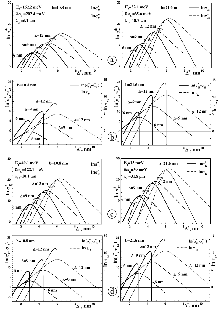
Figure 3: Dependencies of conductivity logarithms $\ln\sigma_{23}^{+}$ , $\ln\sigma_{23}^{-}$ , $\ln\sigma_{12}^{+}$ , $\ln\sigma_{12}^{-}$ , $\ln(\sigma_{23}^{+}-\sigma_{23}^{-})$, $\ln(\sigma_{12}^{+}-\sigma_{12}^{-})$ and life times $\ln\tau_{23}$ , $\ln\tau_{12}$ on output barrier width $\Delta^{+}$ at different well widths $b$ and sum $\Delta$, for the two-barrier RTS operating as detector.

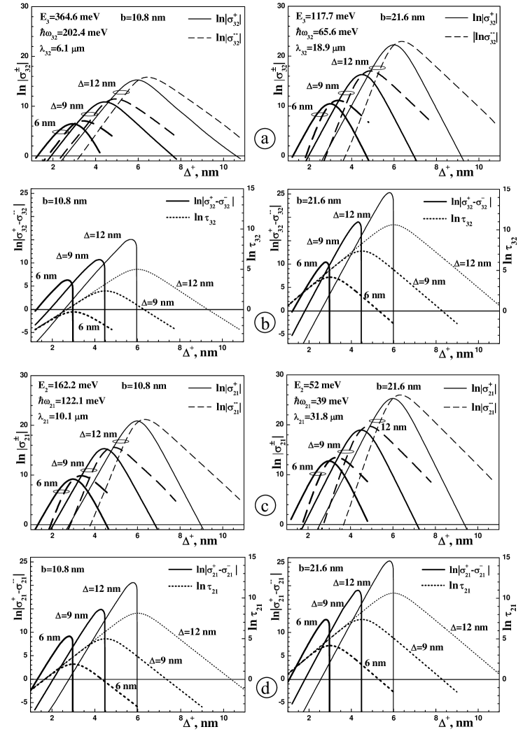
Figure 4: Dependencies of conductivity logarithms $\ln|\sigma_{32}^{+}|$ , $\ln|\sigma_{32}^{-}|$ , $\ln|\sigma_{21}^{+}|$ , $\ln|\sigma_{21}^{-}|$ , $\ln|\sigma_{32}^{+}-\sigma_{32}^{-}|$ , $\ln|\sigma_{21}^{+}-\sigma_{21}^{-}|$ and life times $\ln\tau_{32}$ , $\ln\tau_{21}$ on output barrier width $\Delta^{+}$ at different well width $b$ and sum $\Delta$, for the two-barrier RTS operating as laser.

The developed theory for two-barrier RTS active conductivity is valid for any type of quantum transitions (laser or detector). Further, to optimize the design of the system under research as an active element of nano-laser or nano-detector, there is performed the calculation of electron QSSs life times and maxima of active conductivity together with its components ($\sigma^{-}$, $\sigma^{+}$). The latter are formed by detector transitions with absorption (figure 3) and by laser transitions with radiation (figure 4) of electromagnetic field energy ($\hbar\omega$) with the respective wave-lengths ($\lambda$) shown in figures 3 (a), (c) and 4 (a), (c). The widths of the wells: $b=10.8$ nm, $21.6$ nm and the widths of the barriers: $\Delta=\Delta^{-}+\Delta^{+}=6$ nm, 9 nm, 12 nm were used as typical ones [3, 7, 8, 9, 10] for the experimentally investigated QCDs or QCLs with the range of operating frequencies being in the sub-infrared windows of atmosphere transparency.

The calculated conductivity logarithms: forward $\ln|\sigma_{12(21)}^{+}|$, $\ln|\sigma_{23(32)}^{+}|$ and backward $\ln|\sigma_{12(21)}^{-}|$, $\ln|\sigma_{23(32)}^{-}|$ and their differences $\ln|\sigma_{12(21)}^{+}-\sigma_{12(21)}^{-}|$, $\ln|\sigma_{23(32)}^{+}-\sigma_{23(32)}^{-}|$ (in units $\sigma_{0}=1$ S/cm) formed by the detector ($1\to 2$, $2\to 3$) and laser ($2\to 1$, $3\to 2$) quantum transitions; and logarithms of electron life times sum in operating QSSs $\ln\tau_{n,n\pm 1}$ , where $\tau_{n,n\pm 1}=\tau_{n}+\tau_{n\pm 1}$ (in units $\tau_{0}=1$ s) are presented in figures 3, 4 respectively, as functions of output barrier width $\Delta^{+}$ at the condition of the constant sum of barriers widths: $\Delta=\Delta^{-}+\Delta^{+}=\rm const$ (6 nm, 9 nm, 12 nm).

In figures 3 (a), (c) and 4 (a), (c) one can see that independently of the well width ($b$) and sum of barriers widths ($\Delta$) all $\ln|\sigma_{12}^{\pm}|$, $\ln|\sigma_{23}^{\pm}|$ and $\ln|\sigma_{21}^{\pm}|$, $\ln|\sigma_{32}^{\pm}|$ magnitudes qualitatively similarly depend on the output barrier width ($\Delta^{+}$). Herein, it is evident that $\ln|\sigma_{21}^{\pm}|>\ln|\sigma_{12}^{\pm}|>\ln|\sigma_{32}^{\pm}|>\ln|\sigma_{23}^{\pm}|$. Their main properties are as follows.

The increase of $\Delta^{+}$ (and the corresponding decrease of $\Delta^{-}$) in the range $0<\Delta^{+}<\Delta/2$ causes the linear increase of $\ln|\sigma_{12(21)}^{+}|$, $\ln|\sigma_{23(32)}^{+}|$ and $\ln|\sigma_{12(21)}^{-}|$, $\ln|\sigma_{23(32)}^{-}|$ magnitudes. Herein, there are always satisfied the inequalities: $\ln|\sigma_{12(21)}^{+}|>\ln|\sigma_{12(21)}^{-}|$, $\ln|\sigma_{23(32)}^{+}|>\ln|\sigma_{23(32)}^{-}|$. In the range of output barrier widths $\Delta/2<\Delta^{+}<\Delta$, on the contrary, these magnitudes are linearly decreasing with $\ln|\sigma_{12(21)}^{-}|>\ln|\sigma_{12(21)}^{+}|$, $\ln|\sigma_{23(32)}^{-}|>\ln|\sigma_{23(32)}^{+}|$. In the symmetric two-barrier RTS, when $\Delta^{+}=\Delta^{-}=\Delta/2$, we have $\ln|\sigma_{12(21)}^{+}|=\ln|\sigma_{12(21)}^{-}|$, $\ln|\sigma_{23(32)}^{+}|=\ln|\sigma_{23(32)}^{-}|$ which is completely understandable from physical considerations because the electronic current, after the interaction with the electromagnetic field, flows from the two-barrier RTS by two currents equal over magnitudes and opposite over directions.

The established properties of active conductivity ($\sigma$) and its components ($\sigma_{12(21)}^{+}$, $\sigma_{12(21)}^{-}$ and $\sigma_{23(32)}^{+}$, $\sigma_{23(32)}^{-}$) lead to the evident conclusion. Now it is clear that the condition $|\sigma_{12(21)}^{+}|\gg|\sigma_{12(21)}^{-}|$ or $|\sigma_{23(32)}^{+}|\gg|\sigma_{23(32)}^{-}|$, at which the two-barrier RTS optimally operates as detector or laser, is fulfilled only in the interval of widths $\Delta^{+}<\Delta/2$ ($\Delta/2<\Delta^{-}=\Delta-\Delta^{+}$), i.e., at the ascending parcels of $\ln\sigma_{12(21)}^{+}$ , $\ln\sigma_{23(32)}^{+}$ and $\ln\sigma_{12(21)}^{-}$ , $\ln\sigma_{23(32)}^{-}$ as functions of $\Delta^{+}$. There is performed a calculation of $\ln|\sigma_{12(21)}^{+}-\sigma_{12(21)}^{-}|$, $\ln|\sigma_{23(32)}^{+}-\sigma_{23(32)}^{-}|$ and $\ln\tau_{12}$ , $\ln\tau_{23}$ as functions of $\Delta^{+}$ in order to establish the best ratio between $\Delta^{+}$ and $\Delta^{-}$ magnitudes (at fixed $\Delta=6$ nm, 9 nm, 12 nm). The results are shown in figures 3 (b), (d) and 4 (b), (d).

From figures 3 and 4 one can see that at any $\Delta$, maximum magnitudes of $\ln|\sigma_{12(21)}^{+}-\sigma_{12(21)}^{-}|$, $\ln|\sigma_{23(32)}^{+}-\sigma_{23(32)}^{-}|$ are approached at such widths $\Delta^{+}=\Delta_{m}^{+}$ , which are in the small vicinity from the left hand side of $\Delta^{+}=\Delta/2$. It is clear that as far as the output barrier width $\Delta_{m}^{+}$ is only a little bit smaller than the input barrier width ($\Delta_{m}^{-}=\Delta-\Delta_{m}^{+}$), hence, the forward electronic current through the thinner output barrier is much bigger than the backward current through the thicker input barrier, observed in figure 3 (b), (d) and 4 (b), (d).

For the optimal design of two-barrier RTF and coherent character of electromagnetic wave (in case of laser), the evident physical requirements must be fulfilled: the life time ($\tau_{n,n\pm 1}$) of electron in both operating QSSs should not be bigger than the time ($\tau_{\rm d}$) of dissipative processes (interaction with phonons, impurities and so on). According to the known estimations [3] $\tau_{\rm d}\approx 20$ s or $\ln\tau_{\rm d}\approx 3$. Now, there are obtained the consequent estimations of optimal widths of both barriers $\Delta^{+}$ and $\Delta^{-}$ at which, at the conditions $|\sigma_{12(21)}^{+}|\gg|\sigma_{12(21)}^{-}|$, $|\sigma_{23(32)}^{+}|\gg|\sigma_{23(32)}^{-}|$, the magnitudes $\sigma_{12(21)}$ , $\sigma_{23(32)}$ are maximum due to the linear dependence of $\ln|\sigma_{12(21)}^{+}-\sigma_{12(21)}^{-}|$, $\ln|\sigma_{23(32)}^{+}-\sigma_{23(32)}^{-}|$ and $\ln|\sigma_{12(21)}^{\pm}|$, $\ln|\sigma_{23(32)}^{\pm}|$ maxima on $\Delta$ (figure 3, 4) at fixed well width ($b$). The magnitudes of all evaluated characteristics are shown in figures 3, 4. From the figure one can see that when the well width ($b$) increases, the optimal sum of both barriers widths ($\Delta=\Delta^{+}+\Delta^{-}$), confined by dissipative processes scattering time ($\tau_{\rm d}$) , decreases.

The detection or radiation of electromagnetic field with certain frequency can be obtained due to quantum transitions between QSSs in different two-barrier RTSs with respective widths of potential wells. There arises a question: which one of the two RTSs is more optimal – the one with smaller well width and operating at the transitions between lower levels or the one with bigger well width and operating at the respective transitions between higher levels.

There is an important property of two-barrier RTS, which is really clear from physical considerations. When the electron energy is equal to the resonance energy of any level except the ground one, the quantum transitions into the lower QSSs (figure 4) are more probable than into the higher ones (3). Consequently, the nano-system has a negative conductivity and operates in the regime of electromagnetic field radiation. Thus, in a detector regime, the two-barrier RTS operates only when the energy of electronic current is equal to the resonance energy of ground QSS and quantum transition into the second state occurs with the absorption of electromagnetic field energy. We should note that all the known experimentally utilized nano-detectors operate exactly in this regime [7, 8, 9, 10].

As far as the laser regime is concerned, this is realized within the quantum transitions between the neighbouring levels from arbitrary higher into arbitrary lower states. For example, we can compare the advantages and disadvantages of two different RTS, radiating the electromagnetic field in one of the ranges of atmosphere transparency windows ($\lambda=8-14~{}\mu\rm m$ or $\hbar\omega=89-155$ meV). It is clear from figure 2 (b) that the radiation with the field energy $\hbar\omega=122$ meV can be realized by two two-barrier RTSs with equal barrier widths ($\Delta^{-}=6$ nm, $\Delta^{+}=3$ nm) but different well widths: I) at the transition $2\to 1$ ($b_{I}=10.8$ nm) $\tau_{1}^{I}=14.6$ ps, $\tau_{2}^{I}=1.5$ ps, $\tau_{21}^{I}=\tau_{2}^{I}+\tau_{1}^{I}=16.1$ ps, $E_{2}^{I}=162$ meV, $|\sigma_{21}^{+}|=1200$ S/cm, $|\sigma_{21}^{-}|=1$ S/cm; II) at the transition $3\to 2$ ($b_{II}=15$ nm) $\tau_{2}^{II}=4.7$ ps, $\tau_{3}^{II}=1.1$ ps, $\tau_{32}^{II}=\tau_{3}^{II}+\tau_{2}^{II}=5.8$ ps, $E_{2}^{II}=219$ meV, $|\sigma_{32}^{+}|=811$ S/cm, $|\sigma_{21}^{-}|=2$ S/cm. Comparing the both nano-systems, one can see, even if the life-time ($\tau_{12}^{I}$) of electron in the operating QSS for the system I is almost three times bigger than the life time ($\tau_{32}^{II}$) for the system II, but, herein, the starting electron current ($j_{0}^{I}\sim\sqrt{E_{2}^{I}}$) at system I is 1.2 times smaller than the one ($j_{0}^{II}\sim\sqrt{E_{3}^{II}}$) at the system II. The intensity of radiation, proportional to the conductivity, for the system I is about 1.5 times bigger than for the II system. Thus, the increase of QSSs life times for the system I is not bigger than the scattering times of electrons due to the dissipative processes (phonons, impurities and so on) destroying the coherence. Thus, the optimal two-barrier RTS is the one operating at quantum transitions between two lowest QSSs.

Finally, we should note that the theory for the active conductivity of two-barrier RTS developed within the framework of simple rectangular potentials model and different electron effective masses approximation can be used in future as a basis of investigation and optimization of complicated open RTS with bigger number of wells and barriers, intensively utilized as operating elements of quantum cascade nano-lasers and nano-detectors.

Теорiя активної електронної провiдностi плоскої двобар’єрної наносистеми як робочого елемента квантового каскадного лазера чи детектора М.В. Ткач, Ю.О. Сетi, В.О. Матiєк, О.М. Войцехiвська Чернiвецький нацiональний унiверситет iменi Юрiя Федьковича,
58012 Чернiвцi, вул. Коцюбинського 2

References

- [1] Faist J., Capasso F., Sivco D.L., Sirtori C., Hutchinson A.L., Cho A.Y., Science, 1994, 264, 553; doi:10.1126/science.264.5158.553.
- [2] Faist J., Capasso F., Sirtori C., Appl. Phys. Lett., 1995, 66, 538; doi:10.1063/1.114005.
-
[3]
Gmachl C., Capasso F., Sivco D.L., Cho A.Y.,
Rep. Prog. Phys., 2001, 64, 1533;
doi:10.1088/0034-4885/64/11/204. - [4] Scalari G., Ajili L., Faist J., Beere H., Linfield E., Ritchie D., Davies G., Appl. Phys. Lett., 2003, 82, 3165; doi:10.1063/1.1571653.
- [5] Diehl L., Bour D., Corzine S., Zhu J., Hofler G., Loncar M., Troccoli M., Capasso F., Appl. Phys. Lett., 2006, 88, 201115; doi:10.1063/1.2203964.
- [6] Wang Q.J., Pflug C., Diehl L., Capasso F., Edamura T., Furuta S., Yamanishi M., Kan H., Appl. Phys. Lett., 2009, 94, 011103; doi:10.1063/1.3062981.
- [7] Hofstetter D., Beck M., Faist J., Appl. Phys. Lett., 2002, 81, 2683; doi:10.1063/1.1512954.
- [8] Gendron L., Carras M., Huynh A., Ortiz V., Koeniguer C., Berger V., Appl. Phys. Lett., 2004, 85, 2824; doi:10.1063/1.1781731.
- [9] Giorgetta F.R., Baumann E., Hofstetter D., Manz C., Yang Q., Kohler K., Graf M., Appl. Phys. Lett., 2007, 91, 111115; doi:10.1063/1.2784289.
- [10] Hofstetter D., Giorgetta F.R., Baumann E., Yang Q., Manz C., Kohler K., Appl. Phys. Lett., 2008, 93, 221106; doi:10.1063/1.3036897.
- [11] Elesin V.F., J. Exp. Theor. Phys., 1997, 85, 264; doi:10.1134/1.558273.
- [12] Elesin V.F., Kateev I.Yu., Podlivaev A.I., Semiconductors, 2000, 34, 1321; doi:10.1134/1.1325431.
- [13] Elesin V.F., J. Exp. Theor. Phys., 2002, 94, 794; doi:10.1134/1.1477905.
- [14] Belyaeva I.V., Golant E.I., Pashkovskii A.B., Semiconductors, 1997, 31, 103; doi:10.1134/1.1187090.
-
[15]
Gel’vich E.A., Golant E.I., Pashkovski A.B., Sazonov V.P.,
Tech. Phys. Lett., 1999, 25, 382;
doi:10.1134/1.1262490. - [16] Golant E.I., Pashkovskii A.B., Semiconductors, 2000, 34, 327; doi:10.1134/1.1187981.
- [17] Tkach M.V., Makhanets O.M., Seti Ju.O., Dovganiuk M.M., Voitsekhivska O.M., Acta Phys. Pol. A, 2010, 117, 965.
- [18] Tkach N.V., Seti Yu.A., Low Temp. Phys., 2009, 35, 556; doi:10.1063/1.3170931.