Magnetic breakdown and quantum oscillations in electron-doped high temperature superconductor $\mathrm{Nd_{2-x}Ce_{x}CuO_{4}}$

Abstract

Recent more precise experiments have revealed both a slow and a fast quantum oscillation in the $c$-axis resistivity of nearly optimal to overdoped electron-doped high temperature superconductor $\mathrm{Nd_{2-x}Ce_{x}CuO_{4}}$. Here we study this problem from the perspective of Fermi surface reconstruction using an exact transfer matrix method and the Pichard-Landauer formula. In this method, neither quasiclassical approximations for magnetic breakdown, nor ad hoc broadening of Landau levels, are necessary to study the high field quantum oscillations. The underlying Hamiltonian is a mean field Hamiltonian that incorporates a two-fold commensurate Fermi surface reconsruction. While the specific mean field considered is the $d$-density wave, similar results can also be obtained by a model of a spin density wave, as was explicitly demonstrated earlier. The results are consistent with an interplay of magnetic breakdown across small gaps in the reconstructed Fermi surface and Shubnikov-de Haas oscillations.

I Introduction

Quantum oscillations were first discovered Doiron-Leyraud et al. (2007) in the Hall coefficient of hole-doped high temperature superconductor $\mathrm{YBa_{2}Cu_{3}O_{6+\delta}}$ (YBCO) at high magnetic fields between $35-62T$ in the underdoped regime close to 10%. Since then a number of measurements, in even higher fields and with greater precision using a variety of measurement techniques have confirmed the basic features of this experiment. However, the precise mechanism responsible for oscillations has become controversial. Riggs et al. (2011) Fermi surface reconstruction due to a density wave order that could arise if superconductivity is “effectively destroyed” by high magnetic fields have been focus of some attention. Chakravarty (2008); *Chakravarty:2008b; *Dimov:2008; *Millis:2007; *Yao:2011

In contrast, similar quantum oscillation measurements in the doping range $15-17\%$ in $\mathrm{Nd_{2-x}Ce_{x}CuO_{4}}$ (NCCO) Helm et al. (2009) seem easier to interpret, as the magnetic field range $30-65T$ is far above the upper critical field, which is less than $10T$. This clearly places the material in the “normal” state, a source of contention in measurements in YBCO; in NCCO the crystal structure consists of a single CuO plane per unit cell, and, in contrast to YBCO, there are no complicating chains, bilayers, ortho-II potential, stripes, etc. Armitage et al. (2009) Thus, it would appear to be ideal for gleaning the mechanism of quantum oscillations. On the other hand, disorder in NCCO is significant. It is believed that well-ordered chain materials of YBCO contain much less disorder by comparison.

In a previous publication, Eun et al. (2010) we mentioned in passing that it is not possible to understand the full picture in NCCO without magnetic breakdown effects, since the gaps are expected to be very small in the relevant regime of the parameter space. However, in that preliminary work the breakdown phenomenon was not addressed; instead we focused our attention to the effect of disorder. Since then recent measurements Helm et al. (2010); *Kartsovnik:2011 have indeed revealed magnetic breakdown in the range $16-17\%$ doping, almost to the edge of the superconducting dome. Here we consider the same transfer matrix method used previously, Eun et al. (2010) but include third neighbor hopping of electrons on the square planar lattice, without which many experimental aspects cannot be faithfully reproduced, including quantitative estimates of the oscillation frequencies and breakdown effects. The third neighbor hopping makes the numerical transfer matrix calculation more intensive because of the enlarged size of the matrix, but we were able to overcome the technical challenge. In this paper we also analyze the $c$-axis resistivity and the absence of the electron pockets in the experimental regime.

II Hamiltonian

The mean field Hamiltonian for $d$-density wave Chakravarty et al. (2001) (DDW) in real space, in terms of the site-based fermion annihilation and creation operators $c_{\mathbf{i}}$ and $c_{\mathbf{i}}^{\dagger}$, is

$$H_{DDW}=\sum_{\mathbf{i}}\epsilon_{\mathbf{i}}c_{\mathbf{i}}^{\dagger}c_{\mathbf{i}}+\sum_{\mathbf{i},\mathbf{j}}t_{\mathbf{i},\mathbf{j}}~{}\mathrm{e}^{ia_{\mathbf{i},\mathbf{j}}}c_{\mathbf{i}}^{\dagger}c_{\mathbf{j}}+h.c\\ .,$$ (1)

where the nearest neighbor hopping matrix elements include DDW gap $W_{0}$ and are

$$\begin{split}t_{\mathbf{i},\mathbf{i}+\hat{\mathbf{x}}}&=t+\frac{iW_{0}}{4}(-1)^{(n+m)},\\ t_{\mathbf{i},\mathbf{i}+\hat{\mathbf{y}}}&=t-\frac{iW_{0}}{4}(-1)^{(n+m)},\\ \end{split}$$ (2)

where $(n,m)$ are a pair of integers labeling a site: $\mathbf{i}=n\hat{\mathbf{x}}+m\hat{\mathbf{y}}$; the lattice constant $a$ will be set to unity unless otherwise specified . In this paper we also include both next nearest hopping matrix element, $t^{\prime}$, and third nearest neighbor hopping matrix element $t^{\prime\prime}$. A constant perpendicular magnetic field $B$ is included via the Peierls phase factor $a_{\mathbf{i},\mathbf{j}}=\frac{e}{\hbar c}\int_{\mathbf{j}}^{\mathbf{i}}\mathbf{A}\cdot\mathrm{d}\mathbf{l}$, where $\mathbf{A}=(0,-Bx,0)$ is the vector potential in the Landau gauge. The band parameters are chosen to be $t~{}=~{}0.38eV$, $t^{\prime}~{}=~{}0.32t$, and $t^{\prime\prime}~{}=~{}0.5t^{\prime}$. Pavarini et al. (2001) The chemical potential $\mu$ is adjusted to achieve the required doping level and is given in Table 1, so is the DDW gap $W_{0}$. We assume that the on-site energy is $\delta$-correlated white noise defined by the disorder average $\overline{\epsilon_{\mathbf{i}}}=0$ and $\overline{\epsilon_{\mathbf{i}}\epsilon_{\mathbf{j}}}=V_{0}^{2}\delta_{\mathbf{i},\mathbf{j}}$. Disorder levels for each of the cases studied are also given there in Table 1. We have seen previously that longer ranged correlated disorder lead to very similar results. Jia et al. (2009)

The Fermi surface areas (See Fig. 1) of the small hole pocket in the absence of disorder correspond to oscillation frequencies $330T$ at 15% doping, $317T$ at 16% doping and $291T$ at 17% doping. These frequencies seem to be insensitive to $W_{0}$ within the range given in Table 1.

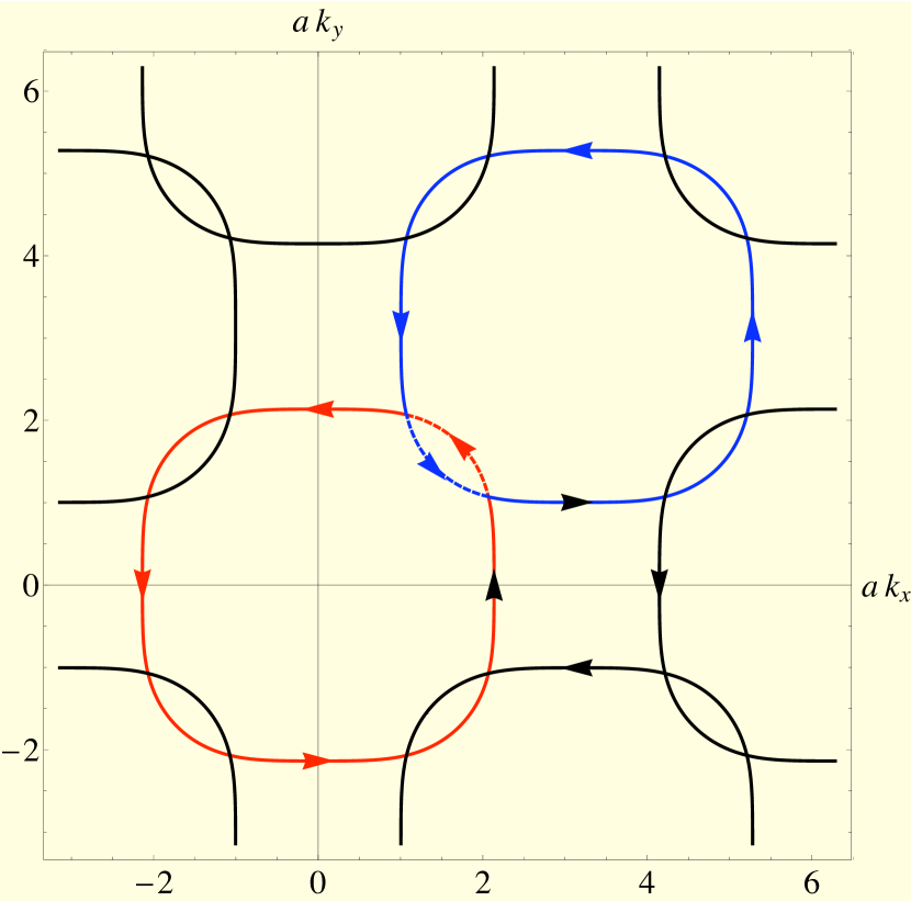
Figure 1: (Color online) A plot showing the breakdown junctions and electron trajectories across them in the extended Brillouin zone. The figure corresponds NCCO with 17% doping and small DDW gap. Note that the reflection at the junctions involve a large change in momentum. The electron trajectories that lead to magnetic breakdown of small hole pockets are shown.

III The transfer matrix method

Transfer matrix to compute the oscillations of the conductance is a powerful method. It requires neither quasiclassical approximation to investigate magnetic breakdown nor does it require ad hoc broadening of the Landau level to incorporate the effect of disorder. Various models of disorder, both long and short-ranged, can be studied ab initio. The mean field Hamiltonian, being a quadratic non-interacting Hamiltonian, leads to a Schrödinger equation for the site amplitudes, which is then recast in the form of a transfer matrix; the full derivation is given in the Appendix. The conductance is then calculated by a formula that is well known in the area of mesoscopic physics, the Pichard-Landauer formula. Pichard and André (1986); *Fisher:1981 This yields Shubnikov-de Haas oscillations of the $ab$-plane resistivity, $\rho_{ab}$. We show later how this can be related to the $c$-axis resistivity $\rho_{c}$ measured in experiments.

Consider a quasi-1D system, $N\gg M$, with a periodic boundary condition along y-direction. Here $Na$ is the length in the $x$-direction and $Ma$ is the length in the $y$-direction, $a$ being the lattice spacing. Let $\Psi_{n}=(\psi_{n,1},\psi_{n,2},\ldots,\psi_{n,M})^{T}$, $n=1,\dots N$, be the amplitudes on the slice $n$ for an eigenstate with a given energy. Then the amplitudes on four successive slices must satisfy the relation

$$\left[\begin{array}[]{c}\Psi_{n+2}\\ \Psi_{n+1}\\ \Psi_{n~{}~{}}\\ \Psi_{n-1}\\ \end{array}\right]=\left[\begin{array}[]{cccc}U_{n}^{-1}A_{n}&U_{n}^{-1}B_{n}&U_{n}^{-1}C_{n}&U_{n}^{-1}D_{n}\\ 1&0&0&0\\ 0&1&0&0\\ 0&0&1&0\\ \end{array}\right]\left[\begin{array}[]{c}\Psi_{n+1}\\ \Psi_{n~{}~{}}\\ \Psi_{n-1}\\ \Psi_{n-2}\\ \end{array}\right]={\mathbf{T}}_{n}\left[\begin{array}[]{c}\Psi_{n+1}\\ \Psi_{n~{}~{}}\\ \Psi_{n-1}\\ \Psi_{n-2}\\ \end{array}\right]$$ (3)

where $U_{n}$, $A_{n}$, $B_{n}$, $C_{n}$, $D_{n}$ are $M\times M$ matrices. The non-zero matrix elements of matrix $A_{n}$ are

$$(A_{n})_{m,m} = -\left[-1-\frac{\mathrm{i}W_{0}}{4}(-1)^{m+n}\right],$$ (4)

$$(A_{n})_{m,m+1} = -t^{\prime}\mathrm{e}^{\mathrm{i}(-n-\frac{1}{2})\phi},$$ (5)

$$(A_{n})_{m,m-1} = -t^{\prime}\mathrm{e}^{\mathrm{i}(n+\frac{1}{2})\phi},$$ (6)

where $\phi=Ba^{2}e/\hbar c$ is a constant. The elements of the matrix $B_{n}$ are

$$(B_{n})_{m,m} = \epsilon_{n,m}-\mu,$$ (7)

$$(B_{n})_{m,m+1} = \left[-1+\frac{\mathrm{i}W_{0}}{4}(-1)^{m+n}\right]\mathrm{e}^{-\mathrm{i}n\phi},$$ (8)

$$(B_{n})_{m,m-1} = \left[-1+\frac{\mathrm{i}W_{0}}{4}(-1)^{m+n}\right]\mathrm{e}^{\mathrm{i}n\phi},$$ (9)

$$(B_{n})_{m,m+2} = t^{\prime\prime}\mathrm{e}^{-\mathrm{i}2n\phi},$$ (10)

$$(B_{n})_{m,m-2} = t^{\prime\prime}\mathrm{e}^{\mathrm{i}2n\phi},$$ (11)

Here $C_{n}=A^{{\dagger}}_{n}$ and $D_{n}=-U_{n}=t^{\prime\prime}\mathbb{1}$, where $\mathbb{1}$ is the $M\times M$ identity matrix.

Table 1: Parameters $W_{0}$ (DDW gap), $V_{0}$ (on-site disorder potential), and $\mu$ (chemical potential).

Figure	Gap $W_{0}$ (meV)	$V_{0}$ (disorder)	$\mu$	doping (%)
Fig. 2	5	$0.2t$	$0.057t$	17
Fig. 3	5	$0.4t$	$0.057t$	17
Fig. 4	5	$0.6t$	$0.057t$	17
Fig. 5	10	$0.2t$	$0.057t$	17
Fig. 6	10	$0.4t$	$0.057t$	17
Fig. 7	10	$0.6t$	$0.057t$	17
Fig. 8	15	$0.2t$	$0.0176t$	16
Fig. 9	15	$0.4t$	$0.0176t$	16
Fig. 10	15	$0.6t$	$0.0176t$	16
Fig. 11	30	$0.2t$	$0.0176t$	16
Fig. 12	30	$0.4t$	$0.0176t$	16
Fig. 13	30	$0.6t$	$0.0176t$	16

The $4M$ Lyapunov exponents, $\gamma_{i}$, of $\lim_{N\to\infty}({\cal T}_{N}{\cal T}_{N}^{\dagger})$, where ${\cal T}_{N}=\prod_{j=1}^{j=N}{\mathbf{T}}_{j}$, are defined by the corresponding eigenvalues $\lambda_{i}=e^{\gamma_{i}}$. All the Lyapunov exponents $\gamma_{1}>\gamma_{2}>\ldots>\gamma_{4M}$, are computed by a method described in Ref. Kramer and Schreiber, 1996. However, the matrix is not symplectic. Therefore all $4M$ eigenvalues are computed. Remarkably, except for a small set, consisting of large eigenvalues, the rest of the eigenvalues do come in pairs $(\lambda,1/\lambda)$, as for the symplectic case, within our numerical accuracy. We have no analytical proof of this curious fact. Clearly, large eigenvalues contribute insignificantly to the Pichard-Landauer Pichard and André (1986) formula for the conductance, $\sigma_{ab}(B)$:

$$\sigma_{ab}(B)=\frac{e^{2}}{h}\text{Tr}\sum_{j=1}^{2M}\frac{2}{({\cal T}_{N}{\cal T}_{N}^{\dagger})+({\cal T}_{N}{\cal T}_{N}^{\dagger})^{-1}+2}.$$ (12)

We have chosen $M$ to be 32, smaller than our previous work. Eun et al. (2010) The reason for this is that the matrix size including the third neighbor hopping is larger $4M\times 4M$ instead of $2M\times 2M$. We chose $N$ to be of the order of $10^{6}$, as before. This easily led to an accuracy better than 5% for the smallest Lyapunov exponent, $\gamma_{i}$, in all cases.

IV Magnetic breakdown and quantum oscillations

We compute the conductance as a function of the magnetic field and then Fourier transform the numerical data. This procedure of course depends on the number of data points sampled within a fixed range of the magnetic field, typically between $45-60T$. As the number of sampling points increases, the peaks become narrower but greater in intensity, conserving the area under the peak. But the location of each peak and the relative ratio of the intensities remain the same. In order to compare the Fourier transformed results, we keep the sampling points fixed in all cases to be 1200.

In Figs. 2 through 4 the results for 17% doping for a $5meV$ gap and varying degrees of disorder are shown. Both the slow oscillation at a frequency $~{}290T$ corresponding to the small hole pocket and $~{}11,700T$ corresponding to the large hole pocket, as schematically sketched in Fig. 1 in the extended Brillouin zone, can be seen. Note that partitioning of the spectral weight between the peaks changes as the degree of disorder is increased. If we change the value of the gap to $10meV$, shown in Figs. 5 through 7, the overall picture remains the same, although the slower frequency peak is a bit more dominant, as the magnetic breakdown is a little less probable. For 16% doping similar calculation with gaps of $15meV$ and $30meV$ also show some evidence of magnetic breakdown depending on the disorder level, particularly seen in $15meV$ data in Figs. 8 though 10. On the other hand, the evidence of magnetic breakdown is much weaker in the $30meV$ data shown in Figs. 11 through 13.

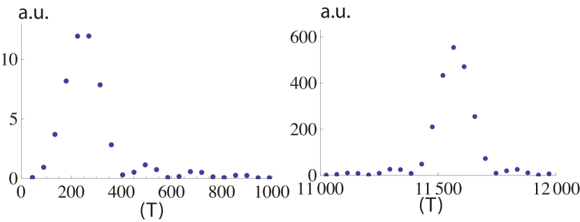
Figure 2: (Color online) Fourier transform of the conductance oscillations with a smooth background term subtracted. The parameters correspond to 17% doping with a DDW gap of $5meV$ and disorder $V_{0}=0.2t$. The horizontal axis is in units of Tesla and the vertical axis is in arbitrary units.

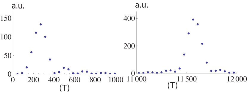
Figure 3: (Color online) The same as in Fig. 2 corresponding to 17% doping but with a DDW gap of $5meV$ and disorder $V_{0}=0.4t$.

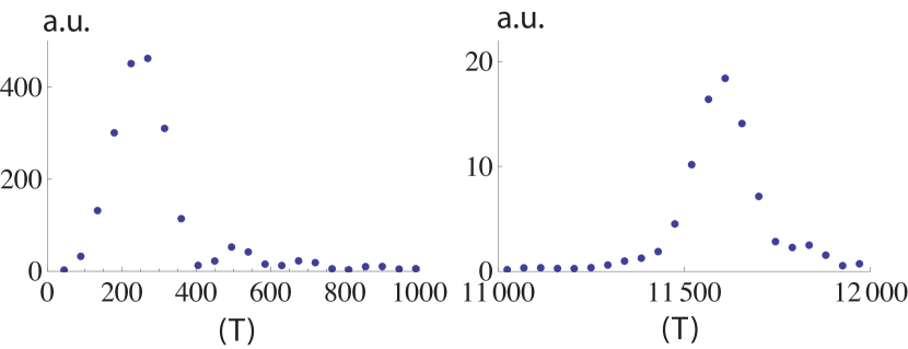
Figure 4: (Color online) The same as in Fig. 2 corresponding to 17% doping but with a DDW gap of $5meV$ and disorder $V_{0}=0.6t$.

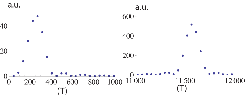
Figure 5: (Color online) The same as in Fig. 2 corresponding to 17% doping but with a DDW gap of $10meV$ and disorder $V_{0}=0.2t$.

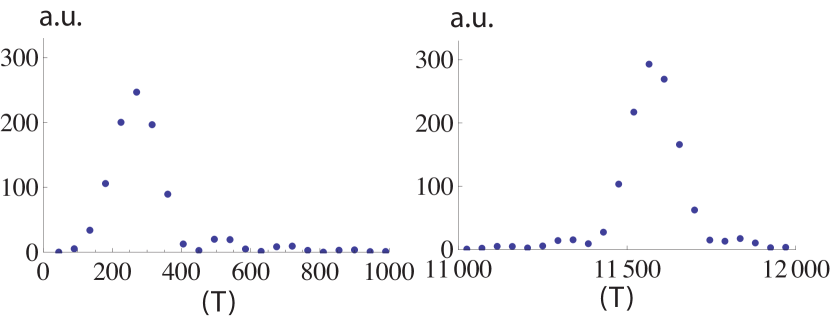
Figure 6: (Color online) The same as in Fig. 2 corresponding to 17% doping but with a DDW gap of $10meV$ and disorder $V_{0}=0.4t$.

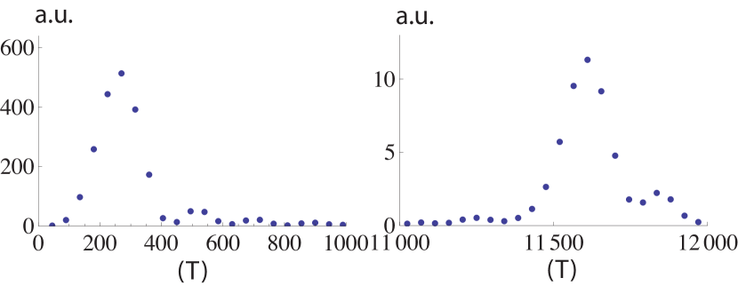
Figure 7: (Color online) The same as in Fig. 2 corresponding to 17% doping but with a DDW gap of $10meV$ and disorder $V_{0}=0.6t$.

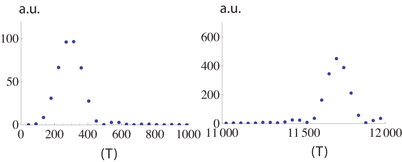
Figure 8: (Color online) The same as in Fig. 2 corresponding to 16% doping but with a DDW gap of $15meV$ and disorder $V_{0}=0.2t$.

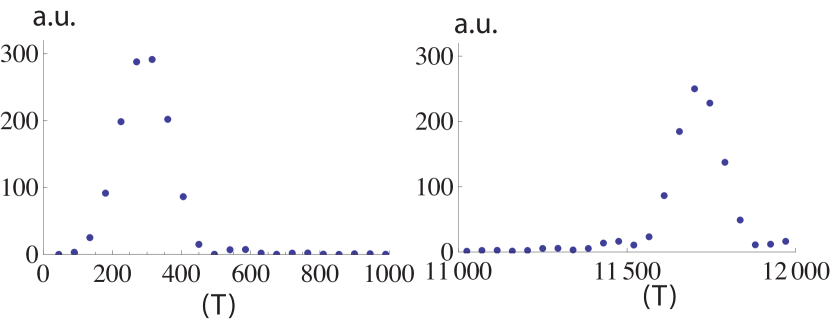
Figure 9: (Color online) The same as in Fig. 2 corresponding to 16% doping but with a DDW gap of $15meV$ and disorder $V_{0}=0.4t$.

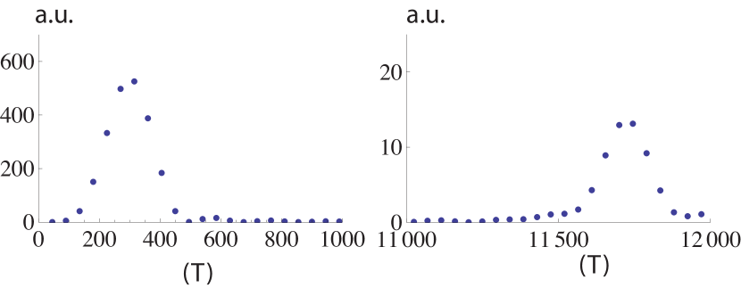
Figure 10: (Color online) The same as in Fig. 2 corresponding to 16% doping but with a DDW gap of $15meV$ and disorder $V_{0}=0.6t$.

Figure 11: (Color online) The same as in Fig. 2 corresponding to 16% doping but with a DDW gap of $30meV$, and disorder $V_{0}=0.2t$.

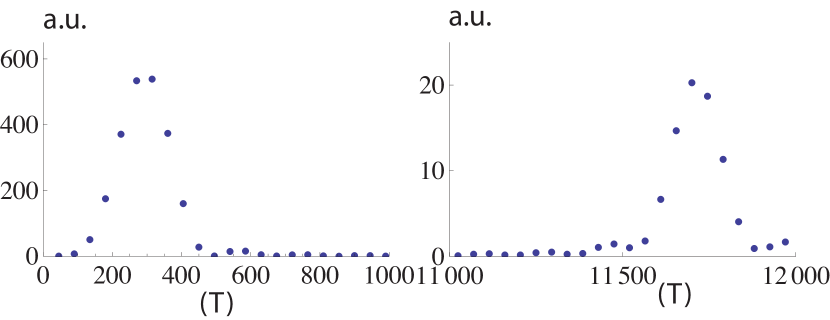
Figure 12: (Color online) The same as in Fig. 2 corresponding to 16% doping but with a DDW gap of $30meV$ and disorder $V_{0}=0.4t$.

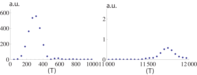
Figure 13: (Color online) The same as in Fig. 2 corresponding to 16% doping but with a DDW gap of $30meV$ and disorder $V_{0}=0.6t$.

It is important to note that in none of these calculations one finds any evidence of the electron pocket centered at $(\pi,0)$ and its symmetry counterparts, which should roughly correspond to a frequency of $2700T$. This is in part due to the fact that the effect of disorder is stronger on the electron pocket Eun et al. (2010) and in part due to the fact that at the breakdown junctions transmission coefficient is larger than the reflection coefficient because it entails a large ($\pi/2$) change in the direction of the momentum; see Fig. 1.

V Oscillations in $c$-axis resistivity

The Pichard-Landauer formula was calculated for conductance oscillations in the $ab$-plane, while the actual measurements in NCCO are carried for the $c$-axis resistivity. It is therefore necessary to relate the two to compare with experiments. A simple description for a strongly layered material can be obtained by modifying an argument of Kumar and Jayannavar. Kumar and Jayannavar (1992) An applied electric field, $E$, along the direction perpendicular to the planes will result in a chemical potential difference

$$\Delta\mu=edE,$$ (13)

where $d$ is the distance between the two planes of an unit cell. The corresponding current, $j_{c}$, is ($\varepsilon_{F}$ is the Fermi energy)

$$j_{c}=e\left[\Delta\mu g_{2D}(\varepsilon_{F},H)\right]\gamma,$$ (14)

since $\Delta\mu g_{2D}(\varepsilon_{F},H)$ is the number of unoccupied states to which an electron can scatter, while $\gamma$ is the scattering rate between the planes of a unit cell. Here, we have included a possible oscillatory dependence of the the two-dimensional density of states, $g_{2D}(\varepsilon_{F},H)$, that gives rise to Shubnikov-de Haas oscillations in the $ab$-plane. Thus,

$$\rho_{c}=\frac{E}{j_{c}}=\frac{1}{e^{2}dg_{2D}(\varepsilon_{F})\gamma}$$ (15)

There is an implicit assumption: an electron from a given plane makes a transition to a continuum of available states with a finite density at the Fermi surface in the next plane. We are not interested in the Rabi oscillations between two discrete states, a process that cannot lead to resistivity.

The measured $ab$-plane resistivity is of the order $10\mu\Omega$-cm as compared $\Omega$-cm for the $c$-axis resistivity even at optimum doping, Armitage et al. (2009) which allows us to make an adiabatic approximation. Because an electron spends much of its time in the plane, making only infrequent hops between the planes, we can adiabatically decouple these two processes. The slower motion along the $c$-axis can be formulated in terms of a $2\times 2$ matrix for each parallel wave vector ${\bf k}_{\parallel}$ after integrating out the planar modes. For simplicity, we are assuming that the $c$-axis warping is negligible, so there are only two available states of the electron corresponding to its locations in the two planes. The excitations in a plane close to the Fermi surface, $k_{\parallel}\approx k_{F,\parallel}$, can be approximated by a bosonic heat bath of particle-hole excitations. In this language, the problem maps on to a two-state Hamiltonian

$$H=-t_{c}\sigma_{x}+\sum_{j}\hbar\omega_{j}b^{\dagger}_{j}b_{j}+\frac{\sigma_{z}}{2}\sum_{j}f_{j}(b^{\dagger}_{j}+b_{j}),$$ (16)

where $\sigma$’s are the standard Pauli matrices and $t_{c}$ is the hopping matrix element between the nearest neighbor planes.. Given the simplification, the sum over ${\bf k}_{\parallel}$ is superfluous, and the problem then maps on to a much studied model of a two-level system coupled to an Ohmic heat bath. Chakravarty and Leggett (1984); *Leggett:1987 The Ohmic nature follows from the fermionic nature of the bath. Chang and Chakravarty (1985)The effect of the bath on the transition between the planest is summarized by a spectral function,

$$J(\omega)=\frac{\pi}{2}\sum_{j}f_{j}^{2}\delta(\omega-\omega_{j}).$$ (17)

For a fermionic bath, we can choose

$$J(\omega)=\begin{cases}2\pi\alpha\omega,\;&\omega\ll\omega_{c}\\ 0,\;&\omega\gg\omega_{c}\end{cases}$$ (18)

where $\omega_{c}$ is a high frequency cutoff, which is of the order of $\omega_{c}=2/\tau_{ab}$, where $\tau_{ab}$ is of the order of the planar relaxation time. For a Fermi bath, the parameter $\alpha$ is necessarily restricted to the range $0\leq\alpha\leq 1$. Chang and Chakravarty (1985) Moreover, for coherent oscillations we must have $\alpha<1/2$. Chakravarty and Leggett (1984) However, we shall leave $\alpha$ as an adjustable parameter, presumably less than or equal to $1/2$ to be consistent with our initial assumptions. While a similar treatment is possible for a non-Fermi liquid, Chakravarty and Anderson (1994) the present discussion is entirely within the Fermi liquid theory.

The quantity $\gamma$ is the interplanar tunneling tunneling rate renormalized by the particle-hole excitations close to the planar Fermi surface and can be easily seen to be Chakravarty and Leggett (1984)

$$\gamma=\frac{2t_{c}}{\hbar}\left(\frac{2t_{c}}{\hbar\omega_{c}}\right)^{\frac{\alpha}{1-\alpha}}.$$ (19)

The $c$-axis resistivity is then

$$\rho_{c}=\frac{\hbar}{e^{2}}\frac{1}{dg_{2D}(\varepsilon_{F},H)\hbar\omega_{c}}\left(\frac{\hbar\omega_{c}}{2t_{c}}\right)^{\frac{1}{1-\alpha}}$$ (20)

This equation can be further simplified by expressing it as a ratio of $\rho_{c}/\rho_{ab}$, but this is unnecessary. Two important qualitative points are: $\rho_{c}$ is far greater than $\rho_{ab}$ and the root of the quantum oscillations of $\rho_{c}$ is quantum oscillations of the planar density of states.

VI Conclusions

We have shown that a qualitatively consistent physical picture for quantum oscillations can be provided with a simple set of assumptions involving reconstruction of the Fermi surface due to density wave order. Although the specific order considered here was the DDW, we have shown previously that at the mean field level a very similar picture can be provided by a two-fold commensurate spin density wave (SDW). Eun et al. (2010) Thus, it appeared unnecessary to repeat the same calculations using the SDW order.

In YBCO, studies involving tilted field seems to rule out triplet order parameter, hence SDW. Ramshaw et al. (2011); *Sebastian:2011 Moreover, from NMR measurements at high fields, there appears to be no evidence of a static spin density wave order in YBCO. Wu et al. (2011) Similarly there is no evidence of SDW order in fields as high as $23.2T$ in $\mathrm{YBa_{2}Cu_{4}O_{8}}$ Zheng et al. (1999), while quantum oscillations are clearly observed in this material. yelland:2008; *Bangura:2008 Also no such evidence of SDW is found up to $44T$ in $\mathrm{Bi_{2}Sr_{2-x}La_{x}CuO_{6+\delta}}$. Kawasaki et al. (2011) At present, results from high field NMR in NCCO does not exist, but measurements are in progress. Brown (2011) It is unlikely that such static SDW order will be revealed in these measurements. This conjecture is based on the zero field neutron scattering measurements which indicate very small spin-spin correlation length in the relevant doping regime. Motoyama et al. (2007) A long range SDW order cannot appear merely by applying high magnetic fields, which is energetically a weak perturbation even for $45T$ field. Nguyen and Chakravarty (2002)

As to singlet order, most likely relevant to the observation of quantum oscillations, Garcia-Aldea and Chakravarty (2011); *Norman:2011; *Ramazashvili:2011 charge density wave is a possibility, which has recently found some support in the high field NMR measurements in YBCO. Wu et al. (2011) But since the mechanism involves oxygen chains, it is unlikely that the corresponding NMR measurements in NCCO will find such a charge order. As to singlet DDW, there are two neutron scattering measurements that seem to provide evidence for it. Mook et al. (2002); *Mook:2004 However, these measurements have not been confirmed by further independent experiments. However, DDW order should be considerably hidden in NMR involving nuclei at high symmetry points, because the orbital currents should cancel.

A mysterious feature of quantum oscillations in YBCO is the fact that only one type of Fermi pockets are observed. If two-fold commensurate density wave is the mechanism, this will violate the Luttinger sum rule. Luttinger (1960); *Chubukov:1997; *Altshuler:1998; *Chakravarty:2008b We have previously provided an explanation for this phenomenon in terms of disorder arising from both defects and vortex scattering in the vortex liquid phase; Jia et al. (2009) however, the arguments are not unassailable. In contrast, for NCCO, the experimental results are quite consistent with the simple theory discussed above. We have not addressed AMRO in NCCO, as the data seem to be somewhat anomalous, Kartsovnik and et al. (2011) although within the Fermi liquid framework discussed here, it should be possible to address this effect in the future.

The basic question as to why Fermi liquid concepts should apply remains an important unsolved mystery. Chakravarty (2011) It is possible that if the state revealed by applying a high magnetic field has a broken symmetry with an order parameter (hence a gap), the low energy excitations will be quasiparticle-like, not a spectra with a branch cut, as in variously proposed strange metal phases. In this respect, the notion of a hidden Fermi liquid may be relevant. Casey and Anderson (2011)

VII Acknowledgments

We thank Mark Kartsovnik, Stuart Brown, Marc-Henri Julien, Brad Ramshaw, and Cyril Proust for keeping us updated regarding their latest experiments. In particular, we thank Marc-Henri Julien for sharing with us his unpublished high field NMR results in YBCO. This work is supported by NSF under the Grant DMR-1004520. *

Appendix A The derivation of the transfer matrix

The DDW Hamiltonian in real space is

$$\begin{split}H=\sum_{\mathbf{i}}\epsilon_{\mathbf{i}}c_{\mathbf{i}}^{\dagger}c_{\mathbf{i}}-t\sum_{\langle\mathbf{i},\mathbf{j}\rangle}~{}\mathrm{e}^{ia_{\mathbf{i},\mathbf{j}}}c_{\mathbf{i}}^{\dagger}c_{\mathbf{j}}-t^{\prime}\sum_{\langle\mathbf{i},\mathbf{j}\rangle^{\prime}}~{}\mathrm{e}^{ia_{\mathbf{i},\mathbf{j}}}c_{\mathbf{i}}^{\dagger}c_{\mathbf{j}}-t^{\prime\prime}\sum_{\langle\mathbf{i},\mathbf{j}\rangle^{\prime\prime}}~{}\mathrm{e}^{ia_{\mathbf{i},\mathbf{j}}}c_{\mathbf{i}}^{\dagger}c_{\mathbf{j}}\\ +\sum_{\mathbf{i}}~{}\frac{iW_{0}}{4}(-1)^{n+m}c_{\mathbf{i}}^{\dagger}c_{\mathbf{\mathbf{i}+\hat{\mathbf{x}}}}-\sum_{\mathbf{i}}~{}\frac{iW_{0}}{4}(-1)^{n+m}c_{\mathbf{i}}^{\dagger}c_{\mathbf{\mathbf{i}+\hat{\mathbf{y}}}}+h.c.\end{split}$$ (21)

Here, $~{}\mathrm{e}^{ia_{\mathbf{i},\mathbf{j}}}$ is the Peierls phase due to the magnetic field. The summation notations are as follows: $\langle\mathbf{i},\mathbf{j}\rangle$, $\langle\mathbf{i},\mathbf{j}\rangle^{\prime}$, and $\langle\mathbf{i},\mathbf{j}\rangle^{\prime\prime}$ imply sum over nearest-neighbor, next-nearest-neighbor, and the third-nearest-neighobor sites, respectively. For example, with the lattice constant set to unity, $\langle\mathbf{i},\mathbf{j}\rangle$ is satisfied when $\mathbf{i}=\mathbf{j}\pm\hat{\mathbf{x}}$ or $\mathbf{i}=\mathbf{j}\pm\hat{\mathbf{y}}$. Likewise, $\langle\mathbf{i},\mathbf{j}\rangle^{\prime}$ requires $\mathbf{i}=\mathbf{j}+\hat{\mathbf{x}}\pm\hat{\mathbf{y}}$ or $\mathbf{i}=\mathbf{j}-\hat{\mathbf{x}}\pm\hat{\mathbf{y}}$ and $\langle\mathbf{i},\mathbf{j}\rangle^{\prime\prime}$ requires $\mathbf{i}=\mathbf{j}\pm 2\hat{\mathbf{x}}$ or $\mathbf{i}=\mathbf{j}\pm 2\hat{\mathbf{y}}$. Here $W_{0}$ is the DDW gap and $\mathbf{i}=(n,m)$. Consider an eigen state $|\Psi\rangle$ with an energy eigenvalue $E$: $H|\Psi\rangle=E|\Psi\rangle$, where $|\Psi\rangle=\sum_{\mathbf{i}}\psi(\mathbf{i})|\mathbf{i}\rangle$; the amplitude at a site is $\psi(\mathbf{i})$. Then the Schrödinger equation can be written in terms of the amplitudes $\psi_{n}(m)$ of the $n$-th slice for all values of $m=1,2,\ldots M$:

$$\begin{split}E\psi_{n}(m)=\epsilon_{\mathbf{i}}\psi_{n}(m)-t\left[\psi_{n+1}(m)+\psi_{n-1}(m)+\mathrm{e}^{-\mathrm{i}n\phi}\psi_{n}(m+1)+\mathrm{e}^{\mathrm{i}n\phi}\psi_{n}(m-1)\right]\\ -t^{\prime}\left[\mathrm{e}^{\mathrm{i}(-n-\frac{1}{2})\phi}\psi_{n+1}(m+1)+\mathrm{e}^{\mathrm{i}(n+\frac{1}{2})\phi}\psi_{n-1}(m+1)+\mathrm{e}^{\mathrm{i}(n+\frac{1}{2})\phi}\psi_{n+1}(m-1)+\mathrm{e}^{\mathrm{i}(-n-\frac{1}{2})\phi}\psi_{n-1}(m-1)\right]\\ -t^{\prime\prime}\left[\psi_{n+2}(m)+\psi_{n-2}(m)+\mathrm{e}^{-\mathrm{i}2n\phi}\psi_{n}(m+2)+\mathrm{e}^{\mathrm{i}2n\phi}\psi_{n}(m-2)\right]\\ +\frac{iW_{0}}{4}(-1)^{n+m}\left[\psi_{n+1}(m)+\psi_{n-1}(m)\right]-\frac{iW_{0}}{4}(-1)^{n+m}\left[\mathrm{e}^{-\mathrm{i}n\phi}\psi_{n}(m+1)+\mathrm{e}^{\mathrm{i}n\phi}\psi_{n}(m-1)\right]\end{split}$$ (22)

With periodic boundary condition along the y-axis i.e. $\psi_{n}(M+1)=\psi_{n}(1)$, the Schrödinger equation can be expressed as a matrix equation:

$$0=-U_{n}\psi_{n+2}+A_{n}\psi_{n+1}+B_{n}\psi_{n}+C_{n}\psi_{n-1}+D_{n}\psi_{n-2},$$ (23)

where $U_{n}$, $A_{n}$, $B_{n}$, $C_{n}$, and $D_{n}$ are $M\times M$ matrices defined in equations following Eq. 3. Now we can solve the Schrodinger equation for $\psi_{n+2}$ to obtain $\psi_{n+2}=U_{n}^{-1}(A_{n}\psi_{n+1}+B_{n}\psi_{n}+C_{n}\psi_{n-1}+D_{n}\psi_{n-2})$. Then the amplitudes at a set of four successive slices, $\psi_{n-1}$ through $\psi_{n+2}$, can be written in terms of the amplitudes of a previous set of four successive slices, $\psi_{n-2}$ through $\psi_{n+1}$. Thus, the transfer matrix in the main text follows.

References

- Doiron-Leyraud et al. (2007) N. Doiron-Leyraud, C. Proust, D. LeBoeuf, J. Levallois, J.-B. Bonnemaison, R. Liang, D. A. Bonn, W. N. Hardy, and L. Taillefer, Nature, 447, 565 (2007).
- Riggs et al. (2011) S. C. Riggs, O. Vafek, J. B. Kemper, J. Betts, A. Migliori, W. N. Hardy, R. Liang, D. A. Bonn, and G. Boebinger, Nat. Phys., 7, 332 (2011).
- Chakravarty (2008) S. Chakravarty, Science, 319, 735 (2008).
- Chakravarty and Kee (2008) S. Chakravarty and H.-Y. Kee, Proc. Natl. Acad. Sci. USA, 105, 8835 (2008).
- Dimov et al. (2008) I. Dimov, P. Goswami, X. Jia, and S. Chakravarty, Phys. Rev. B, 78, 134529 (2008).
- Millis and Norman (2007) A. J. Millis and M. R. Norman, Phys. Rev. B, 76, 220503 (2007).
- Yao et al. (2011) H. Yao, D.-H. Lee, and S. A. Kivelson, “Fermi-surface reconstruction in a smectic phase of a high temperature superconductor,” (2011), arXiv:1103.211v1 [cond-mat] .
- Helm et al. (2009) T. Helm, M. V. Kartsovnik, M. Bartkowiak, N. Bittner, M. Lambacher, A. Erb, J. Wosnitza, and R. Gross, Phys. Rev. Lett., 103, 157002 (2009).
- Armitage et al. (2009) N. P. Armitage, P. Fournier, and R. L. Green, Rev. Mod. Phys., 82, 2421 (2009).
- Eun et al. (2010) J. Eun, X. Jia, and S. Chakravarty, Phys. Rev. B, 82, 094515 (2010).
- Helm et al. (2010) T. Helm, M. V. Kartsovnik, I. Sheikin, M. Bartkowiak, F. Wolff-Fabris, N. Bittner, W. Biberacher, M. Lambacher, A. Erb, J. Wosnitza, and R. Gross, Phys. Rev. Lett., 105, 247002 (2010).
- Kartsovnik and et al. (2011) M. V. Kartsovnik and et al., New J. Phys., 13, 015001 (2011).
- Chakravarty et al. (2001) S. Chakravarty, R. B. Laughlin, D. K. Morr, and C. Nayak, Phys. Rev. B, 63, 094503 (2001).
- Pavarini et al. (2001) E. Pavarini, I. Dasgupta, T. Saha-Dasgupta, O. Jepsen, and O. K. Andersen, Phys. Rev. Lett., 87, 047003 (2001).
- Jia et al. (2009) X. Jia, P. Goswami, and S. Chakravarty, Phys. Rev. B, 80, 134503 (2009).
- Pichard and André (1986) J. L. Pichard and G. André, Europhys. Lett., 2, 477 (1986).
- Fisher and Lee (1981) D. S. Fisher and P. A. Lee, Phys. Rev. B, 23, 6851 (1981).
- Kramer and Schreiber (1996) B. Kramer and M. Schreiber, in Computational Physics, edited by K. H. Hoffmann and M. Schreiber (Springer, Berlin, 1996) p. 166.
- Kumar and Jayannavar (1992) N. Kumar and A. M. Jayannavar, Phys. Rev. B, 45, 5001 (1992).
- Chakravarty and Leggett (1984) S. Chakravarty and A. J. Leggett, Physi. Rev. Lett., 52, 5 (1984).
- Leggett et al. (1987) A. J. Leggett, S. Chakravarty, A. T. Dorsey, M. P. A. Fisher, A. Garg, and W. Zwerger, Rev. Mod. Phys., 59, 1 (1987).
- Chang and Chakravarty (1985) L.-D. Chang and S. Chakravarty, Phys. Rev. B, 31, 154 (1985).
- Chakravarty and Anderson (1994) S. Chakravarty and P. W. Anderson, Phys. Rev. Lett., 72, 3859 (1994).
- Ramshaw et al. (2011) B. J. Ramshaw, B. Vignolle, R. Liang, W. N. Hardy, C. Proust, and D. A. Bonn, Nat. Phys., 7, 234 (2011).
- Sebastian et al. (2011) S. E. Sebastian, N. Harrison, M. M. Altarawneh, F. F. Balakirev, C. H. Mielke, R. Liang, D. A. Bonn, W. N. Hardy, and G. G. Lonzarich, “Direct observation of multiple spin zeroes in the underdoped high temperature superconductor ,” (2011), arXiv:1103.4178v1 [cond-mat] .
- Wu et al. (2011) T. Wu, H. Mayaffre, S. Kramer, M. Horvatic, C. Berthier, W. Hardy, R. Liang, D. Bonn, and M.-H. Julien, “Magnetic-field-induced stripe order in the high temperature superconductor ,” (2011).
- Zheng et al. (1999) G.-q. Zheng, W. G. Clark, Y. Kitaoka, K. Asayama, Y. Kodama, P. Kuhns, and W. G. Moulton, Phys. Rev. B, 60, R9947 (1999).
- Yelland et al. (2008) E. A. Yelland, J. Singleton, C. H. Mielke, N. Harrison, F. F. Balakirev, B. Dabrowski, and J. R. Cooper, Phys. Rev. Lett., 100, 047003 (2008).
- Bangura et al. (2008) A. F. Bangura, J. D. Fletcher, A. Carrington, J. Levallois, M. Nardone, B. Vignolle, P. J. Heard, N. Doiron-Leyraud, D. LeBoeuf, L. Taillefer, S. Adachi, C. Proust, and N. E. Hussey, Phys. Rev. Lett., 100, 047004 (2008).
- Kawasaki et al. (2011) S. Kawasaki, C. Lin, P. L. Kuhns, A. P. Reyes, and G.-q. Zheng, Phys. Rev. Lett., 105, 137002 (2011).
- Brown (2011) S. E. Brown, (2011).
- Motoyama et al. (2007) E. M. Motoyama, G. Yu, I. M. Vishik, O. P. Vajk, P. K. Mang, and M. Greven, Nature, 445, 186 (2007).
- Nguyen and Chakravarty (2002) H. K. Nguyen and S. Chakravarty, Phys. Rev. B, 65, 180519 (2002).
- Garcia-Aldea and Chakravarty (2011) D. Garcia-Aldea and S. Chakravarty, Phys. Rev. B, 82, 184526 (2011).
- Norman and Lin (2011) M. R. Norman and J. Lin, Phys. Rev. B, 82, 060509 (2011).
- Ramazashvili (2011) R. Ramazashvili, Phys. Rev. Lett., 105, 216404 (2011).
- Mook et al. (2002) H. A. Mook, P. Dai, S. M. Hayden, A. Hiess, J. W. Lynn, S. H. Lee, and F. Doǧan, Phys. Rev. B, 66, 144513 (2002).
- Mook et al. (2004) H. A. Mook, P. Dai, S. M. Hayden, A. Hiess, S. H. Lee, and F. Doǧan, Phys. Rev. B, 69, 134509 (2004).
- Luttinger (1960) J. M. Luttinger, Phys. Rev., 119, 1153 (1960).
- Chubukov and Morr (1997) A. V. Chubukov and D. K. Morr, Phys. Rep., 288, 355 (1997).
- Altshuler et al. (1998) B. L. Altshuler, A. V. Chubukov, A. Dashevskii, A. M. Finkel’stein, and D. K. Morr, Europhys. Lett., 41, 401 (1998).
- Chakravarty (2011) S. Chakravarty, Rep. Prog. Phys., 74, 022501 (2011).
- Casey and Anderson (2011) P. A. Casey and P. W. Anderson, Phys. Rev. Lett., 106, 097002 (2011).