Crowding of Polymer Coils and Demixing in Nanoparticle-Polymer Mixtures

Abstract

The Asakura-Oosawa-Vrij (AOV) model of colloid-polymer mixtures idealizes nonadsorbing polymers as effective spheres that are fixed in size and impenetrable to hard particles. Real polymer coils, however, are intrinsically polydisperse in size (radius of gyration) and may be penetrated by smaller particles. Crowding by nanoparticles can affect the size distribution of polymer coils, thereby modifying effective depletion interactions and thermodynamic stability. To analyse the influence of crowding on polymer conformations and demixing phase behaviour, we adapt the AOV model to mixtures of nanoparticles and ideal, penetrable polymer coils that can vary in size. We perform Gibbs ensemble Monte Carlo simulations, including trial nanoparticle-polymer overlaps and variations in radius of gyration. Results are compared with predictions of free-volume theory. Simulation and theory consistently predict that ideal polymers are compressed by nanoparticles and that compressibility and penetrability stabilise nanoparticle-polymer mixtures.

1 Introduction

Colloid-polymer mixtures are among the most actively studied materials because of the windows they open onto the rich physical behaviour of both soft (macromolecular) and hard (atomically ordered) condensed matter. The close analogy between colloidal particles and atoms, combined with real-time imaging of slowly moving particles, have deepened our fundamental understanding of phase transitions, from freezing/melting to the glass transition, gelation, and demixing [1, 2, 3]. With steady advances in nanoparticle synthesis and characterization, much recent interest has turned to the physical properties of nanoparticle-polymer composites [4].

Adding nonadsorbing polymers to a stable suspension of colloids or nanoparticles can induce aggregation and demixing through a depletion mechanism first explained over a half-century ago by Asakura and Oosawa [5]. Depletion of polymers from the space between two particles creates an unbalanced osmotic pressure that drives the particles together. Equivalently, the larger volume available to polymers amidst particles whose excluded-volume shells overlap increases the polymer entropy and manifests as an effective interparticle attraction. Tuning the range and strength of the attraction by varying the polymer size and concentration directly influences phase stability.

The most widely studied model of mixtures of particles and nonadsorbing polymers is the Asakura-Oosawa-Vrij (AOV) model [5, 6], which treats the particles as hard spheres and the polymers as mutually non-interacting (ideal) effective spheres of fixed radius, having hard interactions with the particles. Despite its simplicity, this important reference model succeeds in qualitatively explaining demixing, freezing, and other phenomena observed in real particle-polymer mixtures. Bulk thermodynamic phase behaviour of the AOV model has been intensively explored using thermodynamic perturbation theory [7], free-volume theory [8], and a variety of computational methods. Most simulation studies have been based on Monte Carlo algorithms implemented in either the Gibbs ensemble [9, 10, 11, 12, 13] or the grand canonical ensemble [14, 15, 16], both of which circumvent complications associated with phase interfaces. Quantitative discrepancies between predictions and experiments have motivated enhancements of the AOV model to include more realism in the polymer properties, including polymer-polymer interactions [17, 18, 19, 20, 21, 22, 23, 24], polydispersity in molecular weight [25, 26, 27], and conformational freedom of polymers on a lattice [28, 29]. Recent theoretical and simulation studies of particle-polymer mixtures also have explored interfacial properties [30, 31, 32], demixing in confinement [33, 34, 35, 36, 37, 38], and dynamical properties, such as diffusion and response to shear [23, 24].

A polymer coil has a size that is well characterized by its radius of gyration [39]. Scattering experiments (using, e.g., light or neutrons) probe the mean coil size averaged over an ensemble of conformations. Even for a hypothetical solution having uniform molecular weight (i.e., chain length for linear polymers), the (pre-averaged) radius of gyration exhibits a broad distribution due to statistical fluctuations in coil conformations [40, 41, 42]. This intrinsic polydispersity can influence the phase behaviour of particle-polymer mixtures.

To accommodate intrinsic polymer polydispersity in particle-polymer mixtures, Denton and Schmidt [43] recently proposed a modified AOV model in which the polymer coils have a single internal degree of freedom, namely size. Taking as input the radius of gyration distribution of an ideal polymer coil, they developed and applied a classical density-functional theory, which reduces to a free-volume theory for uniform fluids. In the “colloid” limit, in which the polymer coils are impenetrable to the larger particles, the theory predicts compression of polymer with increasing particle concentration, and a resultant stabilisation of the mixture.

In the “protein” (or nanoparticle) limit, the particles are small enough to penetrate the polymer coils. Recent experiments [44, 45, 46, 47, 48, 49, 50], computer simulations [29, 51, 52, 53], and theories [51, 54, 55, 56] have begun to explore the behaviour of such asymmetric mixtures. These studies raise prospects of modifying protein solutions by adding polymer and tuning properties of polymer-metal (or polymer-semiconductor) nanocomposites by adding nanoparticles to a polymer matrix. Depending on solvent quality and other sample conditions, experiments indicate compression (shrinking) [57, 58], expansion (swelling) [59], or little change in size [60] of polymers in response to nanoparticles. Monte Carlo simulations of bead-spring polymers in the presence of nanoparticles [52, 53] indicate that nanoparticles can penetrate much larger polymer coils. Bulk demixing behaviour has been explored via density-functional theory within a relatively simple model in which the nanoparticles can penetrate the polymers (effective spheres of fixed size) after surmounting an energy barrier [54].

The main purpose of this paper is to study, by means of simulation and theory, the influence of nanoparticles on the conformations of nonadsorbing polymers and the resulting phase stability of nanoparticle-polymer mixtures. Section 2 first defines a simple extension of the AOV model that incorporates nanoparticle-polymer overlap and intrinsic polydispersity in polymer size. Section 3 next outlines our methods: Gibbs ensemble Monte Carlo simulation and a mean-field free-volume theory (with details consigned to appendices). Section 4 presents simulation results and theoretical predictions for polymer size distributions and demixing phase diagrams. Finally, Sec. 5 summarizes and concludes.

2 Model

We consider a mixture of impenetrable nanoparticles and nonadsorbing polymers, dispersed in a solvent, in osmotic equilibrium with a reservoir of pure polymer solution. Exchange of polymers between the system and reservoir (e.g., via a semi-permeable membrane) maintains constant polymer chemical potential. The thermodynamic state of the system is characterized by the temperature $T$, the nanoparticle number density $\rho_{n}$, and the polymer number density in the reservoir $\rho_{p}^{r}$. Equality of polymer chemical potentials in the system and reservoir determines the polymer density in the system $\rho_{p}$.

To model this system, we extend the AOV model to the protein limit in the manner proposed by Schmidt and Fuchs [54] by allowing nanoparticles to penetrate polymers and attributing to each overlapping nanoparticle-polymer pair an energy cost $\epsilon$. With the fixed nanoparticle radius denoted by $R_{n}$ (diameter $\sigma_{n}=2R_{n}$) and the instantaneous radius of a polymer by $R_{p}$, the nanoparticle-nanoparticle and nanoparticle-polymer interactions are specified by pair potentials:

$$v_{nn}(r) = \left\{\begin{array}[]{l@{\quad\quad}l}\infty,&r<\sigma_{n}~{},\\ 0,&r\geq\sigma_{n}~{},\end{array}\right.$$ (3)

$$v_{np}(r) = \left\{\begin{array}[]{l@{\quad\quad}l}\epsilon,&r<R_{n}+R_{p}~{},\\ 0,&r\geq R_{n}+R_{p}~{},\end{array}\right.$$ (6)

where $r$ is the centre-to-centre distance. Assuming ideal polymers, the polymer-polymer interaction vanishes, i.e., $v_{pp}(r)=0$ for all $r$, which strictly applies only to theta solvents [39], wherein the polymer second virial coefficient vanishes.

We further extend the AOV model to describe polymer coils whose size distribution is intrinsically polydisperse [43]. As noted above, even an idealized solution of polymers with uniform chain length has a broad distribution of radius of gyration. In fact, the radius of gyration of an ideal, freely-jointed chain follows the exact probability distribution [61, 62]

$$P_{r}(R_{p}) = \frac{1}{\sqrt{2}\pi R_{g}^{r}t^{3}}\sum_{k=0}^{\infty}\frac{(2k+1)!}{(2^{k}k!)^{2}}(4k+3)^{7/2}\exp(-t_{k})$$ (7)

$$\times \left[\left(1-\frac{5}{8t_{k}}\right)K_{1/4}(t_{k})+\left(1-\frac{3}{8t_{k}}\right)K_{3/4}(t_{k})\right]~{},$$

where

$$R_{g}^{r}~{}=~{}\sqrt{\int_{0}^{\infty}{\rm d}R_{p}\,R_{p}^{2}\,P_{r}(R_{p})}$$ (8)

is the root-mean-square radius of gyration of polymers in the reservoir, $t=(R_{p}/R_{g}^{r})^{2}$, $t_{k}=(4k+3)^{2}/(8t)$, and $K_{n}$ are modified Bessel functions of the second kind.

The extended AOV model is fully specified by the polymer size distribution [equation (7)] and two parameters: the penetration energy $\epsilon$ and the ratio of the rms radius of gyration of polymers in the reservoir to the nanoparticle radius, $q_{r}\equiv R_{g}^{r}/R_{n}$, which is an experimentally accessible property. In the colloid limit ($q_{r}\leq 1$), we assume impenetrable polymers by taking infinite penetration energy ($\epsilon\to\infty$) in equation (6). In the protein limit ($q_{r}\gg 1$), in which the particles can penetrate the polymers, we follow Schmidt and Fuchs [54] and take for the penetration energy an approximation from polymer field theory [63, 64] for the average excess free energy cost of inserting a hard sphere into an ideal coil:

$$\beta\epsilon~{}=~{}\frac{3}{q}~{},$$ (9)

where $\beta\equiv 1/k_{\rm B}T$ and $q\equiv R_{p}/R_{n}$ for a polymer of radius $R_{p}$. The loss of conformational entropy of a polymer that harbours a nanoparticle is thus modelled by an energy penalty that decreases as the polymer swells. (More refined models replace the step-function profile of equation (9) by a continuous function of separation [65, 66].) Next we explore the combined influences of penetration and compressibility on polymer size and demixing.

3 Methods

3.1 Gibbs Ensemble Monte Carlo Simulation

The Gibbs ensemble Monte Carlo (GEMC) method [9, 10, 11, 12, 13] provides a computationally efficient means of computing phase coexistence curves for model fluids. Allowing each phase to occupy a separate box avoids any need to simulate interfaces. This method is known to be of limited accuracy near critical points [67, 68, 69, 70], where grand canonical ensemble methods [14, 15, 16] can yield higher resolution. For our purposes of exploring nanoparticle-polymer demixing, however, GEMC proves practical.

We work in the semigrand ensemble, where temperature, total number of nanoparticles, and total volume, are fixed, while exchange of polymers with a reservoir fixes the polymer chemical potential. The conventional GEMC algorithm for our system involves four types of trial move: (1) displacements of nanoparticles and polymers within each box to ensure thermal equilibrium; (2) exchanges of volume between boxes to ensure mechanical equilibrium, characterized by equality of pressures; (3) transfers of nanoparticles and polymers between boxes to ensure chemical equilibrium, characterized by equality of chemical potentials for each species; and (4) transfers of polymers between each box and the reservoir. The acceptance probabilities for these standard trial moves are given in Appendix A.

To explore the influence of nanoparticles on the polymer size distribution, we implement an additional trial move: variation in polymer radius of gyration $R_{p}$. This move allows the polymer size distribution to adjust to the presence of particles. A polymer coil has radius of gyration $R_{p}$ with probability $P(R_{p})\propto P_{r}(R_{p})\exp(-\beta U)$, where $P_{r}(R_{p})$ is the polymer size distribution of equation (7) and $U$ is the potential energy due to any penetrating particles. A trial change in a polymer’s radius of gyration, from its old value $R_{p}^{o}$ to a new value $R_{p}^{n}$, with an attendant change in potential energy $\Delta U$, is then accepted with probability (see Appendix A)

$${\cal P}_{\rm size}=\min\left\{1,~{}\frac{P_{r}(R_{p}^{n})}{P_{r}(R_{p}^{o})}\exp(-\beta\Delta U)\right\}~{}.$$ (10)

Through trial expansions and contractions, the polymers achieve their equilibrium size distribution. In a dilute suspension of nanoparticles, the size distribution approaches that of the polymer reservoir $P_{r}(R_{p})$. With increasing nanoparticle concentration, however, crowding and penetration influence the polymer size distribution. Exploring the shift in polymer size distribution induced by nanoparticles, and the resulting effect on demixing, is the main goal of our simulation study.

3.2 Simulation Details

We simulated mixtures of nanoparticles and polymers confined to a cubic box (or boxes) with periodic boundary conditions. In the protein limit, we performed GEMC simulations in the semigrand ensemble, with fixed total number of nanoparticles $N_{n}$, total volume $V$, and polymer reservoir density $\rho_{p}^{r}$, for reservoir size ratio $q_{r}=3$. The volumes of the two boxes, initially set equal, were determined by $N_{n}$ and the nanoparticle volume fraction $\eta_{n}=(4\pi/3)\rho_{n}R_{n}^{3}$. In the colloid limit, we performed canonical ensemble simulations (one box), with fixed $N_{n}$, polymer number $N_{p}$, and volume, for $q_{r}=1$ .

The initial configurations were generated by randomly placing particles and polymers (initially monodisperse) on fcc lattice sites. At polymer concentrations exceeding full lattice occupancy, some sites were multiply occupied by polymers. The initial total number of polymers was chosen to yield a desired effective polymer volume fraction, defined as $\eta_{p}=(4\pi/3)\rho_{p}(R_{g}^{r})^{3}$ — an experimentally controllable quantity. From these initial states, the simulations proceeded via the various trial moves outlined in Sec. 3.1. Tolerances were adjusted to yield practical acceptance ratios for each move.

Several diagnostic quantities were calculated to confirm equilibration. The pressure $p$ in each box was computed from a simple adaptation of the virial expression for a binary hard-sphere fluid mixture [71]:

$$\frac{\beta p}{\rho}=1+\frac{2}{3}\pi\rho\left\langle x_{n}^{2}\sigma_{n}^{3}g_{nn}(\sigma_{n})+2(1-e^{-\beta\epsilon})x_{n}\sum_{R_{p}}x_{p}(R_{n}+R_{p})^{3}g_{np}(R_{n}+R_{p})\right\rangle,$$ (11)

where in the given box $\rho$ is the average total number density, $x_{n}$ and $x_{p}$ are the average concentrations of nanoparticles and polymers, $g_{nn}(\sigma_{n})$ and $g_{np}(R_{n}+R_{p})$ are the contact values of the nanoparticle-nanoparticle and nanoparticle-polymer radial distribution functions, the summation runs over all polymer radii, and angular brackets represent an ensemble average over all configurations of nanoparticles and polymers. In practice, the contact values of the radial distribution functions were computed by assigning polymer radii to bins of width $(R_{n}+R_{g}^{r})/50$, accumulating particles in radial bins of width 5% of the radius of the central nanoparticle, and extrapolating to contact.

The chemical potential of the nanoparticles was computed using Widom’s test particle insertion method [72], applied to trial nanoparticle transfers:

$$\beta\mu_{n}=-\ln\left\langle\frac{V/\sigma_{n}^{3}}{N_{n}+1}\exp(-\beta\Delta U)\right\rangle,$$ (12)

where $\Delta U$ is the change in potential energy of the box into which a nanoparticle is inserted and $\langle~{}\rangle$ represents an ensemble average over all configurations. In the semigrand ensemble, the chemical potentials of polymers of all sizes are imposed by the reservoir. As a consistency check, the mean polymer chemical potential (averaged over polymer sizes) also was computed via Widom’s insertion method applied to trial polymer transfers:

$$\beta\mu_{p}=-\ln\left\langle\frac{V/\sigma_{n}^{3}}{N_{p}+1}\exp(-\beta\Delta U)\right\rangle,$$ (13)

where $\Delta U$ now is the change in potential energy upon insertion of a polymer. Note that the chemical potentials are defined relative to an arbitrary reference potential, determined by the choice of volume units (here $\sigma_{n}^{3}$).

For comparison with free-volume theory (Sec. 3.3), we also computed the effective fraction of the total volume (averaged over polymer sizes) that was accessible to the polymers, i.e., not excluded by the nanoparticles. At equilibrium, the chemical potentials of polymer in the system and reservoir must be equal. Thus, equating $\mu_{p}$ [from equation (13)] to the mean chemical potential of (ideal) polymers in the reservoir,

$$\beta\mu_{p}^{r}=\ln\left(\rho_{p}^{r}\sigma_{n}^{3}\right)=\ln\left(\rho_{p}\sigma_{n}^{3}/\alpha_{\rm eff}\right)~{},$$ (14)

the effective polymer free-volume fraction amidst nanoparticles can be expressed as

$$\alpha_{\rm eff}=\rho_{p}\left\langle\frac{V}{N_{p}+1}\exp(-\beta\Delta U)\right\rangle~{}.$$ (15)

The effective polymer free-volume fraction for a given box was determined by applying equation (15) during the GEMC simulation and averaging over all trial polymer transfers into the box.

3.3 Free-Volume Theory

To guide the choice of parameters in our simulations, we generalize the free-volume theory of Lekkerkerker et al [8] to the case of compressible, penetrable polymers. As shown in Appendix B, the Helmholtz free energy density $f$ of a mixture of nanoparticles of number density $\rho_{n}$ (volume fraction $\eta_{n}$) and polymers in osmotic equilibrium with a polymer reservoir of density $\rho_{p}^{r}$ can be expressed (in $k_{B}T$ units) as

$$f(\eta_{n},\rho_{p}^{r})=\rho_{n}\left[\ln\left(\rho_{n}\sigma_{n}^{3}\right)-1\right]+\phi_{hs}(\eta_{n})+\rho_{p}^{r}\alpha_{\rm eff}(\eta_{n})\left[\ln\left(\rho_{p}^{r}\sigma_{n}^{3}\right)-1\right]~{},$$ (16)

where

$$\alpha_{\rm eff}(\eta_{n})\equiv\int_{0}^{\infty}{\rm d}R_{p}\,P_{r}(R_{p})\alpha(R_{p};\eta_{n})$$ (17)

is the effective free-volume fraction of the polymers amidst nanoparticles of volume fraction $\eta_{n}$ [cf. equation (15)], expressed as a weighted average of the free-volume fraction $\alpha(R_{p};\eta_{n})$ of polymers of radius $R_{p}$. The first two terms on the right side of equation (16) are the ideal-gas and excess free energy densities of the hard-sphere nanoparticles; the third term is the total free energy density of the polymers. Note that in this mean-field approximation, which neglects nanoparticle-polymer correlations, $\alpha(R_{p};\eta_{n})$ and $\alpha_{\rm eff}(\eta_{n})$ are assumed to be independent of the polymer density. The corresponding polymer size distribution in the mixture is given by (see Appendix B)

$$P(R_{p};\eta_{n})=\frac{\alpha(R_{p};\eta_{n})}{\alpha_{\rm eff}(\eta_{n})}P_{r}(R_{p})~{}.$$ (18)

4 Results and Discussion

We initialized the GEMC simulations with $N_{n}=400$ nanoparticles and $N_{p}=1000$ polymers in a volume yielding a nanoparticle volume fraction of $\eta_{n}=0.03$. After equilibrating for 150,000 MC cycles, statistics were accumulated and averaged over the next 150,000 cycles. Equilibrium was diagnosed via equality of pressures and chemical potentials in coexisting phases. Several longer runs for larger systems confirmed that equilibrium was attained and that finite-size effects were negligible. The main simulation results reported below are coexistence densities of nanoparticle and polymer species and probability distributions (histograms) of polymer radius.

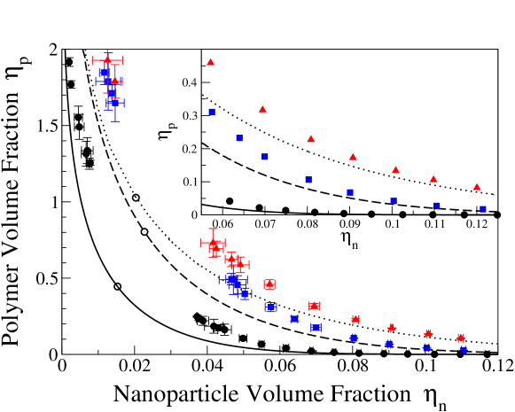
Figure 1: Phase diagram of a nanoparticle-polymer mixture in osmotic equilibrium with a reservoir of polymers whose mean radius of gyration is three times the nanoparticle radius ($q_{r}=3$). Symbols represent simulation data and curves predictions of free-volume theory for nanoparticle-rich and -poor binodals (open circles are predicted critical points). Results are shown for three polymer models: AOV model with impenetrable, incompressible polymer (black circles, solid curve); penetrable, incompressible polymer (blue squares, dashed curve); and penetrable, compressible polymer (red triangles, dotted curve). Inset: expanded view of nanoparticle-rich phase.

Figure 1 shows the fluid-fluid demixing phase diagram for reservoir polymer-to-nanoparticle size ratio $q_{r}=3$ (nanoparticle limit). In this representation, the polymer volume fraction in the system (rather than in the reservoir) is plotted on the vertical axis, facilitating comparison with experiment. Corresponding points on the nanoparticle-rich and -poor branches of the binodal represent coexisting “liquid” and “vapour” phases. The demixing and freezing transitions being well separated for this size ratio, we need not consider the liquid-solid phase boundary. Results are shown for the AOV model and its two penetrable-polymer extensions (incompressible and compressible polymers). Numerical data from our simulations are plotted together with predictions from our free-volume theory calculations, derived from a coexistence analysis that equates pressures and chemical potentials in each phase [using the free energy of equation (16)].

The simulations indicate that polymer penetrability and compressibility both promote stability against demixing, raising the binodal relative to that of the AOV model. The free-volume theory predicts the same qualitative trend, but somewhat underestimates stability of the mixture — a result of neglecting nanoparticle-polymer correlations. The theory also predicts an increase in critical polymer concentration with added polymer freedom. Although this prediction is impractical to test with the Gibbs ensemble method, it could be tested by grand canonical ensemble methods.

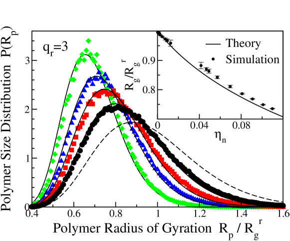
Figure 2: Probability distribution of polymer radius of gyration in a mixture of nanoparticles and penetrable, compressible polymers in osmotic equilibrium with a polymer reservoir. The mean radius of polymer in the reservoir is three times the nanoparticle radius ($q_{r}=3$). Polymer size distributions are shown along the liquid and vapour binodals for polymer chemical potentials $-\beta\mu_{p}=0.9$, 1.3, 1.5, and 1.7 (left to right), corresponding to mean nanoparticle volume fractions $\eta_{n}=0.120$, 0.0809, 0.0572, and 0.0312. The symbols are simulation data, solid curves are predictions of free-volume theory, and the dashed curve is the reservoir size distribution (pure polymer solution). Inset: Ratio of mean polymer radius of gyration in the system $R_{g}\equiv\left\langle R_{p}^{2}\right\rangle^{1/2}$ [equation (19)] to radius of gyration in the reservoir $R_{g}^{r}$ (see Table 1).

Polymer radius of gyration distributions (normalized histograms) are shown in Fig. 2 over a range of polymer chemical potentials along the liquid-vapour binodal. Our simulation data (smoothed by a running average) are compared with theoretical predictions from equation (18). The size distribution is seen to shift towards smaller radii of gyration with increasing nanoparticle concentration, reflecting compression of polymers due to crowding and penetration by nanoparticles. Endowing each polymer with the internal freedom to change its radius of gyration allows the polymers to shrink (compress) to avoid penetration by nanoparticles and contributes to stabilising the mixture. Polymer compression is further quantified by the mean radius of gyration,

$$R_{g}(\eta_{n})=\left\langle R_{p}^{2}\right\rangle^{1/2}=\left(\Delta R_{p}\sum_{i}\,P(R_{p}^{(i)};\eta_{n})(R_{p}^{(i)})^{2}\right)^{1/2},$$ (19)

defined as an average over conformations, i.e., sum over histogram bins, where $R_{p}^{(i)}$ is the polymer radius at bin $i$, and $\Delta R_{p}$ is the bin width. The corresponding polymer compression ratios $R_{g}/R_{g}^{r}$ are plotted in the inset of Fig. 2 and listed in Table 1.

Table 1: Polymer compression ratio $R_{g}(\eta_{n})/R_{g}^{r}$ for reservoir polymer-to-nanoparticle size ratio $q_{r}=R_{g}^{r}/R_{n}=3$ (see inset to Fig. 2). Results of Monte Carlo simulations are compared with predictions of free-volume theory over a range of nanoparticle volume fractions $\eta_{n}$ and polymer volume fractions $\eta_{p}$ along the demixing binodal.

$\eta_{n}$	$\eta_{p}$	Simulation	Theory
0.002	3.21	0.987 $\pm$ 0.001	0.991
0.009	2.17	0.968 $\pm$ 0.005	0.963
0.013	1.93	0.959 $\pm$ 0.011	0.948
0.042	0.731	0.882 $\pm$ 0.011	0.859
0.049	0.587	0.863 $\pm$ 0.007	0.841
0.057	0.459	0.842 $\pm$ 0.005	0.822
0.069	0.317	0.811 $\pm$ 0.004	0.796
0.081	0.227	0.786 $\pm$ 0.002	0.773
0.091	0.173	0.768 $\pm$ 0.001	0.754
0.100	0.133	0.749 $\pm$ 0.001	0.739
0.110	0.106	0.735 $\pm$ 0.001	0.723
0.120	0.082	0.720 $\pm$ 0.002	0.707

To further explore polymer compression, we performed canonical ensemble (constant-$NVT$) simulations in the colloid limit ($q_{r}=1$) at fixed polymer volume fraction. Polymer size distributions and compression ratios are shown over a range of particle volume fractions in Fig. 3. For dilute suspensions, crowding by particles compresses the polymers, as for $q_{r}=3$. These results support the trends in polymer size distribution predicted previously [43] for the same compressible polymer model. With increasing particle concentration, however, the polymers cease shrinking and begin to expand. This size reversal can be understood by noting that the trajectory of the state point now crosses the binodal from the stable (mixed) region into the unstable (demixed) region of the phase diagram. Snapshots of the system in the unstable region reveal the presence of large polymer clusters. Within such a cluster, polymers are shielded from particles and thus are free to adopt a size distribution closer to that in the reservoir. Such correlation-driven behaviour clearly is not captured by the mean-field theory.

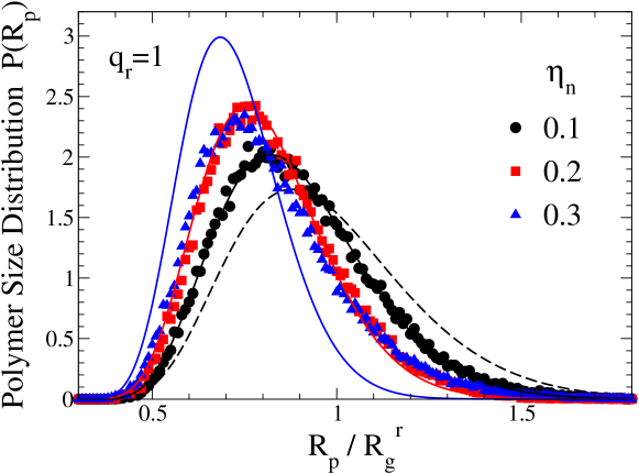
Figure 3: Probability distribution of polymer radius of gyration $R_{p}$ in a mixture of particles and impenetrable, but compressible, polymer at fixed polymer volume fraction $\eta_{p}=0.1$. The mean radius of polymer in the reservoir is equal to the particle radius ($q_{r}=1$). Simulation data (symbols) and predictions of free-volume theory (curves) are shown for increasing particle volume fraction $\eta_{n}=0$, 0.1, 0.2, and 0.3 (right to left).

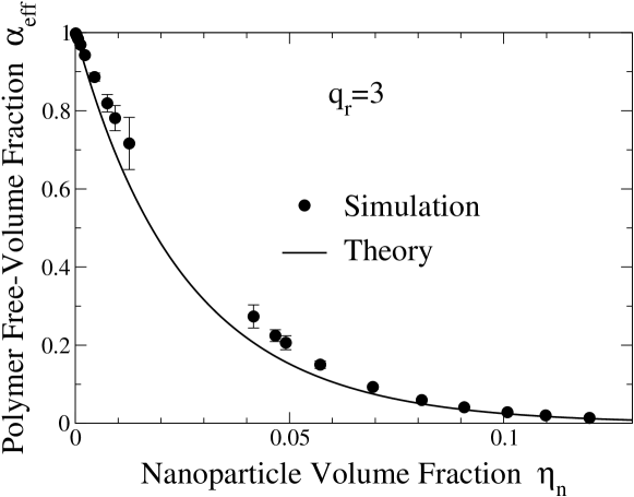
Figure 4: Effective polymer free-volume fraction $\alpha_{\rm eff}$ in a mixture of nanoparticles and penetrable, compressible polymer in osmotic equilibrium with a polymer reservoir for reservoir polymer-to-nanoparticle size ratio $q_{r}=3$. The symbols are simulation data [equation (15)] and the curve is the prediction of free-volume theory [Eq. (17)] along the liquid and vapour (demixing) binodals.

The influence of polymer compressibility on phase behaviour can be interpreted also in terms of effective interactions between nanoparticles induced by polymer depletion. Note that compression of polymers by crowding shortens the range of depletion-induced attraction between nanoparticles to an extent that depends on particle concentration. Since polymers in the nanoparticle-rich phase are more compressed, on average, than those in the nanoparticle-poor phase, weakening of the effective attraction tends to stabilise the nanoparticle-rich phase against demixing.

Figure 4 finally presents results for the polymer free-volume fraction $\alpha$, computed from equations (15) and (17), along the binodal of Fig. 1. Polymer compression clearly increases the free-volume fraction accessible to the polymers, consistent with the shift of the nanoparticle-rich binodal towards higher polymer volume fractions. The free-volume theory captures the qualitative trend, but underestimates $\alpha$ at higher nanoparticle concentrations, again because of neglect of nanoparticle-polymer correlations.

5 Summary and Conclusions

In summary, we have performed Monte Carlo simulations of model mixtures of monodisperse hard-sphere nanoparticles and nonadsorbing, intrinsically polydisperse polymers in a theta solvent. The polymers are modeled as effective spheres, each with a single internal degree of freedom (average size), which allows for fluctuations in radius of gyration. In addition to conventional Monte Carlo moves, the polymers undergo trial size variations, with an acceptance probability dependent on nanoparticle concentration. Within this coarse-grained model, we have investigated the effect of nanoparticle crowding on polymer size and the influence of polymer compression and penetrability on the demixing behaviour of nanoparticle-polymer mixtures.

For particles and polymers of comparable size, our simulations confirm the trends previously predicted by density-functional theory [43], namely that particles compress the polymer coils and that mixing stability is enhanced by polymer compression. In equilibrium fluid-fluid coexistence, the polymers fractionate into compressed coils in the particle-rich phase and expanded coils in the particle-poor phase. In the protein limit, in which nanoparticles face an energy barrier for penetrating the larger polymers, our simulations also show significant polymer compression and enhanced stability, in qualitative agreement with predictions of free-volume theory. Incorporating into the model excluded-volume interactions between polymer segments may help to shed light on the conformations of crowded polymers in good solvents.

While our model includes intrinsic polydispersity of polymers, it neglects polydispersity in chain length (molecular weight), which can be significant in real polymer systems [25, 26, 27]. Fasolo and Sollich [27] have applied free-volume theory to mixtures of particles and polydisperse polymers, finding that polydispersity in chain length promotes demixing – an effect just opposite to that of polymer compressibility. The relative importance of these two competing effects could be assessed by combining, in a single model, both radius of gyration and chain length polydispersities.

Finally, we emphasize that the present study demonstrates a general and practical approach to modelling soft matter systems, in which the microscopic complexity of the constituent macromolecules is considerably reduced through a coarse-grained approximation, while physically relevant features are retained and subsumed into a small number of internal degrees of freedom. Conceptual insight provided by this mesoscopic approach may help to guide the design of experiments and the choice of parameters in studies of more detailed molecular models [29, 52, 53]. A similar analysis of polymer shape variations induced by particle crowding, and the influence on demixing behaviour, will be the subject of future work.

Appendix A Acceptance Probabilities of Monte Carlo Trial Moves

The acceptance probabilities for the GEMC trial moves follow directly from the condition of detailed balance [73], according to which the average rate of transition from an old state ($o$) to a new state ($n$) must equal, in equilibrium, the average transition rate from state $n$ to state $o$. Defining $P(o)$ and $P(n)$ as the probabilities of finding the system in the states $o$ and $n$, respectively, and $\pi(o\to n)$ as the transition probability between the states, detailed balance requires that

$$P(o)\pi(o\to n)=P(n)\pi(n\to o)~{}.$$ (20)

Assuming that trial moves $o\to n$ and $n\to o$ are attempted at equal rates, equation (20) implies acceptance probabilities in the ratio

$$\frac{{\rm acc}(o\to n)}{{\rm acc}(n\to o)}=\frac{P(n)}{P(o)}~{}.$$ (21)

In the Metropolis algorithm, trial moves are accepted with probability [73, 74]

$${\cal P}(o\to n)=\min\left\{1,~{}\frac{P(n)}{P(o)}\right\}~{}.$$ (22)

Trial displacements of randomly chosen particles are thus accepted with probability

$${\cal P}_{\rm disp}=\min\left\{1,~{}\exp(-\beta\Delta U)\right\}~{},$$ (23)

where $\Delta U=U_{n}-U_{o}$ is the change in energy between old and new configurations. A trial move leading to overlap of nanoparticles yields infinite $\Delta U$ and so is automatically rejected. Each nanoparticle-polymer overlap increases $U$ by $\epsilon$; otherwise $\Delta U=0$.

In the semigrand Gibbs ensemble, box $i$ holds $N_{i}$ particles in a volume $V_{i}$ ($i=1,2$). A trial exchange of volume $\Delta V$, achieved by uniformly rescaling all particle coordinates, such that $V_{1}\to V_{1}+\Delta V$ and $V_{2}\to V_{2}-\Delta V$, is accepted with probability

$${\cal P}_{\rm vol}=\min\left\{1,~{}\left(\frac{V_{1}+\Delta V}{V_{1}}\right)^{N_{1}}\left(\frac{V_{2}-\Delta V}{V_{2}}\right)^{N_{2}}\exp(-\beta\Delta U)\right\}~{}.$$ (24)

In practice, it proves more efficient to make trial moves in $\ln(V_{1}/V_{2})$, for which the acceptance probability is [73, 74]

$${\cal P}_{\rm vol}=\min\left\{1,~{}\left(\frac{V_{1}+\Delta V}{V_{1}}\right)^{N_{1}+1}\left(\frac{V_{2}-\Delta V}{V_{2}}\right)^{N_{2}+1}\exp(-\beta\Delta U)\right\}~{}.$$ (25)

Denoting by $N_{j1}$ and $N_{j2}$ the respective particle numbers of species $j$ ($j=n,p$) in the two boxes, transfer of a particle of species $j$ from box 1 to box 2, resulting in $N_{j1}\to N_{j1}-1$ and $N_{j2}\to N_{j2}+1$, is accepted with probability [11]

$${\cal P}_{\rm trans}=\min\left\{1,~{}\frac{N_{j1}V_{2}}{(N_{j2}+1)V_{1}}\exp(-\beta\Delta U)\right\}.$$ (26)

In the colloid limit ($q_{r}\leq 1$), because of the difficulty of inserting a large particle into a box without overlaps, only direct transfers of polymers between the two boxes were attempted. Transfers of particles were achieved indirectly by exchanging identities of particles and polymers [12, 13]. In an identity-exchange move, a randomly chosen polymer in a randomly chosen box is changed to a particle; in the other box, a randomly chosen particle is changed to a polymer. Changing a polymer to a particle in box 1 (and a particle to a polymer in box 2) is accepted with probability

$${\cal P}_{\rm ex}=\min\left\{1,~{}\frac{N_{p1}N_{n2}}{(N_{n1}+1)(N_{p2}+1)}\exp[-\beta(\Delta U_{1}+\Delta U_{2})]\right\}~{},$$ (27)

where $N_{n1}$ ($N_{p1}$) and $N_{n2}$ ($N_{p2}$) are the respective numbers of particles (polymers) in the two boxes and $\Delta U_{1}$ and $\Delta U_{2}$ are the resulting changes in energy in boxes 1 and 2 – incremented by $\epsilon$ for each overlap of a particle and a polymer.

Trial transfers of polymer between the system and the reservoir are attempted with equal frequencies in either direction. Transfer of a polymer from the reservoir to the system is executed as follows. A polymer with a radius chosen randomly from the reservoir size distribution is placed at a random position in a randomly chosen box. For a transfer from the reservoir to box 1, the acceptance probability is

$${\cal P}_{\rm res}=\min\left\{1,~{}\frac{\rho_{p}^{r}V_{1}}{N_{p1}+1}\exp(-\beta\Delta U_{1})\right\}~{},$$ (28)

where $\Delta U_{1}$ is the change in energy of box 1. Transfer of a polymer from the system to the reservoir proceeds by removing a randomly chosen polymer from a randomly chosen box, with acceptance probability

$${\cal P}_{\rm res}=\min\left\{1,~{}\frac{N_{p1}-1}{\rho_{p}^{r}V_{1}}\exp(-\beta\Delta U_{1})\right\}~{}.$$ (29)

Finally, from equation (22), a trial change in polymer size from radius $R_{p}^{o}$ to $R_{p}^{n}$ is accepted with a probability given by equation (10). The same result follows also from the general relation ${\cal P}(o\to n)=\min\left\{1,\exp(-\beta\Delta F)\right\}$, where $\Delta F$ is the change in Helmholtz free energy, if the conformational entropy of a polymer in the system is taken to be the same as in the reservoir, i.e., $-k_{\rm B}T\ln P_{r}(R_{p})$.

Appendix B Free-Volume Theory of Nanoparticle-Polymer Mixtures

Following [8, 43], the Helmholtz free energy density $f$ of a mixture of nanoparticles of number density $\rho_{n}$ (volume fraction $\eta_{n}$) and polymers in osmotic equilibrium with a polymer reservoir of density $\rho_{p}^{r}$ can be expressed (in $k_{B}T$ units) as

$$f(\eta_{n},\rho_{p}^{r})=\rho_{n}\left[\ln\left(\rho_{n}\sigma_{n}^{3}\right)-1\right]+\phi_{hs}(\eta_{n})+f_{p}(\eta_{n},\rho_{p}^{r})~{},$$ (30)

to within an arbitrary constant. The excess free energy density of the hard-sphere nanoparticles is accurately approximated by the Carnahan-Starling expression [71]:

$$\phi_{hs}(\eta_{n})=\rho_{n}\frac{\eta_{n}(4-3\eta_{n})}{(1-\eta_{n})^{2}}~{}.$$ (31)

Progress in approximating the polymer free energy density $f_{p}$ is facilitated by defining polymer density distributions $\rho_{p}(R_{p};\eta_{n})$ and $\rho_{p}^{r}(R_{p})$, in the system and reservoir, respectively. These density distributions are related to the corresponding polymer size distributions, $P(R_{p};\eta_{n})$ and $P_{r}(R_{p})$, according to

$$\rho_{p}(R_{p};\eta_{n})=\rho_{p}(\eta_{n})P(R_{p};\eta_{n})\quad{\rm and}\quad\rho_{p}^{r}(R_{p})=\rho_{p}^{r}P_{r}(R_{p})~{},$$ (32)

which are normalized such that

$$\rho_{p}(\eta_{n})=\int_{0}^{\infty}{\rm d}R_{p}\,\rho_{p}(R_{p};\eta_{n})\quad{\rm and}\quad\rho_{p}^{r}=\int_{0}^{\infty}{\rm d}R_{p}\,\rho_{p}^{r}(R_{p})$$ (33)

are the average polymer densities in the system and reservoir, respectively.

In free-volume theory, the polymer free energy is approximated by the sum of the free energy of an ideal gas of polymers confined to the free volume, i.e., the volume not excluded by the nanoparticles, and the entropy of a polymer coil due to internal (conformational) degrees of freedom:

$$f_{p}=\int_{0}^{\infty}{\rm d}R_{p}\,\rho_{p}(R_{p};\eta_{n})\left[\ln\left(\frac{\rho_{p}(R_{p};\eta_{n})\sigma_{n}^{3}}{\alpha(R_{p};\eta_{n})}\right)-1+f_{\rm conf}(R_{p})\right]~{},$$ (34)

where $\alpha(R_{p};\eta_{n})$ is the free-volume fraction of polymers of radius $R_{p}$ amidst nanoparticles of volume fraction $\eta_{n}$ and $f_{\rm conf}(R_{p})$ is the conformational entropy of a polymer coil. Now equality of polymer chemical potentials in the system and reservoir implies

$$\rho_{p}(R_{p};\eta_{n})=\rho_{p}^{r}(R_{p})\alpha(R_{p};\eta_{n})~{}.$$ (35)

Furthermore, assuming the conformational entropy of a polymer in the system is the same as in the reservoir, we have

$$f_{\rm conf}(R_{p})=-\ln P_{r}(R_{p})~{}.$$ (36)

Combining equations (32)-(36), the polymer free energy density is given by

$$f_{p}(\eta_{n};\rho_{p}^{r})=\rho_{p}^{r}\alpha_{\rm eff}(\eta_{n})\left[\ln\left(\rho_{p}^{r}\sigma_{n}^{3}\right)-1\right]~{},$$ (37)

with the effective polymer free-volume fraction $\alpha_{\rm eff}(\eta_{n})$ defined by equation (17). Equations (30) and (37) together yield the total free energy density of equation (16). Moreover, from equations (32), (33), and (35), the polymer size distribution in the system is expressed by equation (18).

In practice, it is convenient to approximate the reservoir polymer size distribution [equation (7)] by the accurate, analytic ansatz of Eurich and Maass [75]:

$$P_{r}(u)=\frac{1}{2uK_{0}}\exp\left(-\frac{u}{a}-d^{2}\frac{a}{u}\right)~{},$$ (38)

where $u\equiv R_{p}^{2}$, $K_{0}=0.015923$, $a=0.0802$, and $d=1.842$ (see equation (13) in [75]). For the polymer free-volume fraction, we adapt the geometry-based approximation of Oversteegen and Roth [76]:

$$\alpha(R_{p};\eta_{n})=(1-\eta_{n}^{\prime})\exp[-\beta(pv_{p}+\gamma a_{p}+\kappa c_{p})]~{},$$ (39)

where $\eta_{n}^{\prime}\equiv[1-\exp(-\beta\epsilon)]\eta_{n}$ represents an effective nanoparticle volume fraction for penetrable polymers [54]. Equation (39), a generalization of scaled-particle theory derived from the fundamental measures formulation of density-functional theory [77, 78, 79] conceptually separates thermodynamic properties of the nanoparticle hard-sphere fluid — bulk pressure $p$, surface tension at a planar hard wall $\gamma$, and bending rigidity $\kappa$ — from geometric properties of the polymer depletant — volume $v_{p}=(4\pi/3)R_{p}^{3}=(4\pi/3)R_{n}^{3}q^{3}$, surface area $a_{p}=4\pi R_{p}^{2}=4\pi R_{n}^{2}q^{2}$, and integrated mean curvature $c_{p}=R_{p}=R_{n}q$. The hard-sphere properties are approximated by the Carnahan-Starling expressions [76]:

$$\beta p = \frac{3\eta_{n}^{\prime}}{4\pi R_{n}^{3}}\frac{1+\eta_{n}^{\prime}+\eta_{n}^{\prime 2}-\eta_{n}^{\prime 3}}{(1-\eta_{n}^{\prime})^{3}}$$

$$\beta\gamma = \frac{3}{4\pi R_{n}^{2}}\left[\frac{\eta_{n}^{\prime}(2-\eta_{n}^{\prime})}{(1-\eta_{n}^{\prime})^{2}}+\ln(1-\eta_{n}^{\prime})\right]$$

$$\beta\kappa = \frac{3\eta_{n}^{\prime}}{R_{n}(1-\eta_{n}^{\prime})}~{}.$$ (40)

References

- [1] Pusey P N 1991 Liquids, Freezing and Glass Transition ed Hansen J-P, Levesque D, and Zinn-Justin J (Amsterdam: North-Holland)
- [2] Poon W C K 2002 J. Phys.: Condens. Matter14, R859 (2002).
- [3] Tuinier R, Rieger J, and de Kruif C G 2003 Adv. Colloid Interface Sci. 103 1
- [4] Balazs A C, Emrick T, and Russell T P 2006 Science 314 1107
- [5] Asakura S and Oosawa F 1954 J. Chem. Phys.22 1255
- [6] Vrij A 1976 Pure and Appl. Chem. 48 471
- [7] Gast A P, Russel W B and Hall C K 1986 J. Coll. Int. Sci. 109 161
- [8] Lekkerkerker H N W, Poon W C K, Pusey P N, Stroobants A, and Warren P B 1992 Europhys. Lett. 20 559
- [9] Panagiotopoulos A Z 2000 J. Phys.: Condens. Matter12 R25
- [10] Panagiotopoulos A Z 1987 Mol. Phys. 61 813
- [11] Panagiotopoulos A Z, Quirke N, Stapleton M, and Tildesley D J 1988 Mol. Phys. 63 527
- [12] Panagiotopoulos A Z 1989 Int. J. Thermophys. 4 739
- [13] Panagiotopoulos A Z 1995 Observation, Prediction, and Simulation of Phase Transitions in Complex Fluids, NATO ASI Series C 460 463-501 ed Baus M, Rull L R, and Ryckaert J P (Dordrecht: Kluwer)
- [14] Vink R L C and Horbach J 2004 J. Phys.: Condens. Matter16 S3807
- [15] Vink R L C and Horbach J 2004 J. Chem. Phys.121 3253
- [16] Lo Verso F, Vink R L C, Pini D, and Reatto L 2006 Phys. Rev.E 73 061407
- [17] Louis A A, Bolhuis P G, Hansen J-P, and Meijer E J 2000 Phys. Rev. Lett.85 2522
- [18] Bolhuis P G, Louis A A, and Hansen J-P 2002 Phys. Rev. Lett.89 128302
- [19] Schmidt M and Denton A R 2002 Phys. Rev.E 65 21508
- [20] Schmidt M, Denton A R, and Brader J M 2003 J. Chem. Phys.118 1541
- [21] Tuinier R, Aarts D G A L, Wensink H H, and Lekkerkerker H N W 2003 Phys. Chem. Chem. Phys. 5 3707
- [22] Rosch T W and Errington J R 2008 J. Chem. Phys.129 164907
- [23] Zausch J, Virnau P, Binder K, Horbach J, and Vink R L C 2009 J. Chem. Phys.130 064906
- [24] Zausch J, Horbach J, Virnau P, and Binder K 2011 J. Phys.: Condens. Matter22 104120
- [25] Sear R P and Frenkel D 1997 Phys. Rev.E 55 1677
- [26] Warren P B 1997 Langmuir 13 4588
- [27] Fasolo M and Sollich P 2005 J. Phys.: Condens. Matter17 797
- [28] Meijer E J and Frenkel D 1991 Phys. Rev. Lett.67 1110; 1994 J. Chem. Phys.100 6873; 1995 Physica A 213 130
- [29] Chou C-Y, Vo T T M, Panagiotopoulos A Z, and Robert M 2006, Physica A 369 275
- [30] Moncho-Jordá A, Rotenberg B, and Louis A A 2003 J. Chem. Phys.119 12667
- [31] Vink R L C and Schmidt M 2005 Phys. Rev.E 71 051406
- [32] Dijkstra M, van Roij R, Roth R, and Fortini A 2006 Phys. Rev.E 73 041404
- [33] Schmidt M, Fortini A, Dijkstra M 2003 J. Phys.: Condens. Matter15 S3411
- [34] Fortini A, Schmidt M, Dijkstra M 2006 Phys. Rev.E 73 051502
- [35] Vink R L C, Binder K, and Horbach J 2006 Phys. Rev.E 73 056118
- [36] Vink R L C, De Virgilis A, Horbach J, and Binder K 2006 Phys. Rev.E 74 031601
- [37] De Virgilis A, Vink R L C, Horbach J, and Binder K 2007 Europhys. Lett. 77 60002
- [38] De Virgilis A, Vink R L C, Horbach J, and Binder K 2008 Phys. Rev.E 78 1539
- [39] de Gennes P G 1979 Scaling Concepts in Polymer Physics (Ithaca: Cornell)
- [40] Fixman M 1962 J. Chem. Phys.36 306
- [41] Flory P J and Fisk S 1966 J. Chem. Phys.44 2243
- [42] Flory P J 1969 Statistical Mechanics of Chain Molecules (New York: Wiley)
- [43] Denton A R and Schmidt M 2002 J. Phys.: Condens. Matter14 12051
- [44] Caseri W 2000 Macromol. Rapid Commun. 21 705
- [45] Ramakrishnan S, Fuchs M, Schweizer K S, and Zukoski C F 2002 Langmuir 18 1082
- [46] Ramakrishnan S, Fuchs M, Schweizer K S, and Zukoski C F 2002 J. Chem. Phys.116 2201
- [47] Shaw S A, Chen Y L, Schweizer K S, and Zukoski C F 2003 J. Chem. Phys.118 3350
- [48] Kramer T, Schweins R, and Huber K 2005 J. Chem. Phys.123 14903
- [49] Kramer T, Schweins R, and Huber K 2005 Macromol. 38 9783
- [50] Hennequin Y, Evens M, Quezada Angulo C M, and van Duijneveldt J S 2005 J. Chem. Phys.123 54906
- [51] Moncho-Jordá A, Louis A A, Bolhuis P G, and Roth R 2003 J. Phys.: Condens. Matter15 S3429
- [52] Doxastakis M, Chen Y-L, Guzmán O, and de Pablo J J 2004 J. Chem. Phys.120 9335.
- [53] Doxastakis M, Chen Y-L, and de Pablo J J 2005 J. Chem. Phys.123 34901.
- [54] Schmidt M and Fuchs M 2002 J. Chem. Phys.117 6308
- [55] Bolhuis P G, Meijer E J, and Louis A A 2003 Phys. Rev. Lett.90 68304
- [56] Belotelov V I, Carotenuto G, Nicolais L, Pepe G P, and Zvezdin A K 2005 Eur. Phys. J. B 45 317
- [57] Kramer T, Schweins R, and Huber K 2005 Macromol. 38 151
- [58] Le Coeur C, Demé B, and Longeville S 2009 Phys. Rev.E 79 031910
- [59] Tuteja A, Duxbury P M, and Mackay M E 2008 Phys. Rev. Lett.100 077801
- [60] Sen S, Xie Y, Kumar S K, Yang H, Bansal A, Ho D L, Hall L, Hooper J B, and Schweizer K S 2007 Phys. Rev. Lett.98 128302
- [61] Fujita H and Norisuye T 1970 J. Chem. Phys.52 1115
- [62] Yamakawa H 1970 Modern Theory of Polymer Solutions (New York: Harper & Row)
- [63] Eisenriegler E, Hanke A, and Dietrich S 1996 Phys. Rev.E 54 1134
- [64] Hanke A, Eisenriegler E, and Dietrich S 1999 Phys. Rev.E 59 6853
- [65] Woodward C E and Forsman J 2008 Phys. Rev. Lett.100 98301
- [66] Forsman J and Woodward C E 2009 J. Chem. Phys.131 044903
- [67] Valleau J P 1998 J. Chem. Phys.108 2962
- [68] Potoff J J and Panagiotopoulos A Z 1998 J. Chem. Phys.109 10914
- [69] Errington J R 2003 J. Chem. Phys.118 9915
- [70] Hynninen A-P and Panagiotopoulos A Z 2008 Mol. Phys. 106 2039
- [71] Hansen J-P and McDonald I R 1990 Theory of Simple Liquids (New York: Academic)
- [72] Widom B J 1963 J. Chem. Phys.39 2808
- [73] Frenkel D and Smit B 2001 Understanding Molecular Simulation (London: Academic)
- [74] Allen M P and Tildesley D J 1987 Computer Simulation of Liquids (Oxford: Oxford)
- [75] Eurich F and Maass P 2001 J. Chem. Phys.11 7655
- [76] Oversteegen S M and Roth R 2005 J. Chem. Phys. 122 214502
- [77] Rosenfeld Y 1989 Phys. Rev. Lett.63 980
- [78] Rosenfeld Y 1994 Phys. Rev.E 50 R3318
- [79] Schmidt M, Löwen H, Brader J M, and Evans R 2000 Phys. Rev. Lett.85 1934.