The instability transition for the restricted 3-body problem
III. The Lyapunov exponent criterion

Abstract

Aims. We establish a criterion for the stability of planetary orbits in stellar binary systems by using Lyapunov exponents and power spectra for the special case of the circular restricted 3-body problem (CR3BP). The criterion augments our earlier results given in the two previous papers of this series where stability criteria have been developed based on the Jacobi constant and the hodograph method.

Methods. The centerpiece of our method is the concept of Lyapunov exponents, which are incorporated into the analysis of orbital stability by integrating the Jacobian of the CR3BP and orthogonalizing the tangent vectors via a well-established algorithm originally developed by Wolf et al. The criterion for orbital stability based on the Lyapunov exponents is independently verified by using power spectra. The obtained results are compared to results presented in the two previous papers of this series.

Results. It is shown that the maximum Lyapunov exponent can be used as an indicator for chaotic behaviour of planetary orbits, which is consistent with previous applications of this method, particularly studies for the Solar System. The chaotic behaviour corresponds to either orbital stability or instability, and it depends solely on the mass ratio $\mu$ of the binary components and the initial distance ratio $\rho_{0}$ of the planet relative to the stellar separation distance. Detailed case studies are presented for $\mu=0.3$ and 0.5. The stability limits are characterized based on the value of the maximum Lyapunov exponent. However, chaos theory as well as the concept of Lyapunov time prevents us from predicting exactly when the planet is ejected. Our method is also able to indicate evidence of quasi-periodicity.

Conclusions. For different mass ratios of the stellar components, we are able to characterize stability limits for the CR3BP based on the value of the maximum Lyapunov exponent. This theoretical result allows us to link the study of planetary orbital stability to chaos theory noting that there is a large array of literature on the properties and significance of Lyapunov exponents. Although our results are given for the special case of the CR3BP, we expect that it may be possible to augment the proposed Lyapunov exponent criterion to studies of planets in generalized stellar binary systems, which is strongly motivated by existing observational results as well as results expected from ongoing and future planet search missions.

1 Introduction

A classical problem within the realm of orbital stability studies for theoretical and observed planets in stellar binary systems is the circular restricted 3-body problem (CR3BP) (e.g., Szebehely 1967; Roy 2005). The CR3BP describes the motion of a body of negligible mass moving in the gravitational field of the two massive primaries considered here to be two stars. The stars move in circular orbits about the center of mass and their motion is not influenced by the third body, the planet. Furthermore, the initial velocity of the planet is assumed in the same direction as the orbital velocity of its host star, which is usually the more massive of the two stars.

The study of planetary orbital stability is timely for various astronomical reasons. First, although most planets are found in wide binaries, various cases of planets in binaries with separation distances of less than 30 AU have also been identified (e.g., Patience et al. 2002; Eggenberger et al. 2004; Eggenberger & Udry 2010, and references therein). Second, many more cases of planets in stellar binary systems are expected to be discovered noting that binary (and possibly multiple) stellar systems occur in high frequency in the local Galactic neighbourhood (Duquennoy & Mayor 1991; Lada 2006; Raghavan et al. 2006). Moreover, orbital stability studies of planets around stars, including binary systems, are highly significant in consideration of ongoing and future planet search missions (e.g., Catanzarite et al. 2006; Cockell et al. 2009).

The CR3BP has been studied in detail by Dvorak (1984), Dvorak (1986), Rabl & Dvorak (1988), Smith & Szebehely (1993), Pilat-Lohinger & Dvorak (2002), and Mardling (2007). It has also been the focus of the previous papers in this series. In Paper I, Eberle et al. (2008) obtained the planetary stability limits using a criterion based on Jacobi’s integral and Jacobi’s constant. The method, also related to the concept of Hill stability (Roy 2005), showed that orbital stability can be guaranteed only if the initial position of the planet lies within a well-defined limit determined by the mass ratio of the stellar components. Additionally, the stability criterion was found to be also related to the borders of the “zero velocity contour” (ZVC) and its topology assessed by using a synodic coordinate system regarding the two stellar components.

In Paper II, Eberle & Cuntz (2010) followed another theoretical concept based on the hodograph eccentricity criterion. This method relies on an approach given by differential geometry that analyzes the curvature of the planetary orbit in the synodic coordinate system. The centerpiece of this method is the evaluation of the effective time-dependent eccentricity of the orbit based on the hodograph in rotating coordinates as well as the calculation of the mean and median values of the eccentricity distribution. This approach has been successful in mapping quasi-periodicity and multi-periodicity for planets in binary systems. It has also been tested by comparing its theoretical predictions with work by Holman & Wiegert (1999) and Musielak et al. (2005) in regard to the extent of the region of orbital stability in binary systems of different mass ratios.

Previously, the work by Eberle & Cuntz (2010) dealt with the assessment of short-time orbital stability, encompassing time scales of 10³ yrs or less. One of the findings was the identification of a quasi-periodic region in the stellar mass and distance ($\mu$, $\rho_{0}$) parameter space (see Sect. 2.1). Due to the relatively short time scales considered in the previous study, there is a strong motivation to revisit the onset of orbital instability using longer time scales and different types of methods. The focus of this paper is the analysis of orbital stability by Lyapunov exponents, which are among the most commonly used numerical tools for investigating chaotic behaviour of different dynamical systems (e.g., Hilborn 1994). The exponents have already repeatedly been used in orbital mechanics studies of the Solar System (e.g., Lissauer 1999; Murray & Holman 2001). For example, Lissauer (1999) discussed the long-term stability of the eight Solar System planets, while also considering previous studies. He concluded that the Solar System is most likely astronomically stable, in the view of the limited life time of the Sun; however, the orbits of Pluto and of many asteroids may become unstable soon after the Sun becomes a white dwarf.

The numerical procedure of computing the Lyapunov exponents has been developed by Wolf et al. (1985) based on previous work by Benettin et al. (1980). Hence, the main objective of the present paper is to establish the Lyapunov exponent criterion and verify it by performing the power spectra analysis (e.g., Hilborn 1994) as well as by comparing the obtained results to those presented in Paper I and II. Our newly established criterion is then used to investigate the stability of planetary orbits in stellar binary systems (approximated here as the CR3BP) of different mass and distance ratios. The methodology of our study of orbital stability based on the Lyapunov exponent criterion is presented and discussed in §2. Detailed model simulations are described in §3, and our conclusions are given in §4.

2 Theoretical approach

2.1 Basic equations

In the following, we consider the so-called coplanar CR3BP (e.g., Szebehely 1967; Roy 2005), which we will define as follows. Two stars are in circular motion about their common center of mass and their masses are much larger than the mass of the planet. In our case, the planetary mass is assumed to be $1\times 10^{-6}$ of the mass of the star it orbits; also note that the planetary motion is constrained to the orbital plane of the two stars. Moreover, it is assumed that the initial velocity of the planet is in the same direction as the orbital velocity of its host star, which is the more massive of the two stars, and that the starting position of the planet is to the right of the primary star (3 o’clock position), along the line joining the binary components.

Following the conventions described by Eberle et al. (2008), we write the equations of motion in terms of the parameters $\mu$ and $\rho_{0}$ with $\mu$ and $\alpha=1-\mu$ being related to the ratio of the two stellar masses $m_{1}$ and $m_{2}$ (see below). Moreover, $R_{0}$ denotes the initial distance of the planet from its host star, the more massive of the two stars with mass $m_{1}$, whereas $D$ denotes the distance between the two stars, allowing us to define $\rho_{0}$. In addition, we use a rotating reference frame, which also gives rise to Coriolis and centrifugal forces. The equations of motion are given as

$$\dot{x} = u$$ (1)

$$\dot{y} = v$$ (2)

$$\dot{z} = w$$ (3)

$$\dot{u} = 2v+x-\alpha{x-\mu\over r_{1}^{3}}-\mu{x+\alpha\over r_{2}^{3}}$$ (4)

$$\dot{v} = -2u+y-\alpha{y\over r_{1}^{3}}-\mu{y\over r_{2}^{3}}$$ (5)

$$\dot{w} = -\alpha{z\over r_{1}^{3}}-\mu{z\over r_{2}^{3}}$$ (6)

where

$$\mu = {m_{2}\over m_{1}+m_{2}}$$ (7)

$$\alpha = 1-\mu$$ (8)

$$r_{1}^{2} = \left(x-\mu\right)^{2}+y^{2}+z^{2}$$ (9)

$$r_{2}^{2} = \left(x+\alpha\right)^{2}+y^{2}+z^{2}$$ (10)

$$\rho_{0} = {R_{0}\over D}$$ (11)

The variables in the above equations describe the position of the planet, which in essence constitutes a test particle. Its position is defined in Cartesian coordinates $\left\{x,\;y,\;z\right\}$. We denote the time derivative or velocity of a coordinate using the dot notation $\left\{\dot{x}={\rm dx\over dt}\right\}$. We also represent the set of second order differential equations, the equations of motion, by a set of first order differential equations. The velocity is defined by the coordinates $\left\{u,\;v,\;w\right\}$ whose time derivatives are the accelerations. By defining the mass ratio and using normalized coordinates, we can define the distances $\left\{r_{1},\;r_{2}\right\}$ with reference to the location of the stars in the rotating coordinate system.

We enumerate the co-linear Lagrange points in the synodic frame by the order of which the ZVC opens. The point between the stars opens first; therefore, we denote it as L1. The point to the left of the star that does not host the planet opens second; thus, we denote it L2. The point to the right of the star hosting the planet opens third and it is denoted L3. The two Trojan Lagrange points which are of lesser importance to our study are L4 and L5 (see Fig. 1).

2.2 Lyapunov exponents

A fundamental difference between stable and unstable planetary orbits is that two nearby trajectories in phase space will diverge as a power law (usually linear) for the former and exponentially for the latter. The parameter that is used to measure this rate of divergence is called Lyapunov exponent as it was originally introduced by Lyapunov (1907); see also Baker & Gollub (1990). A dynamical system with n degrees of freedom is represented in 2n phase space; thus, to fully determine the stability of the system all 2n Lyapunov exponents must be calculated. The Lyapunov exponents are the most commonly used tools to determine the onset of chaos and chaotic behaviour of both dissipative (e.g., Musielak & Musielak 2009, and references therein) and non-dissipative systems of orbital mechanics (e.g., Lissauer 1999, and references therein). The positive Lyapunov exponents measure the rate of divergence of neighbouring orbits, whereas negative exponents measure the convergence rates between stable manifolds. For dissipative dynamical systems the sum of all Lyapunov exponents is less than $0$ (e.g., Musielak & Musielak 2009); however, for Hamiltonian (non-dissipative) systems the sum is equal to $0$ (e.g., Hilborn 1994).

Specific applications of the Lyapunov exponents to the circular restricted 3-body problem were discussed by many authors, including Gonczi & Froeschlé (1981), Jefferys & Yi (1983), Lecar et al. (1992), Milani & Nobili (1992), Smith & Szebehely (1993), Murray & Holman (2001), and others. Some of these authors also considered the so-called Lyapunov time, which measures the $e$-folding time for the divergence of nearby trajectories. It should be noted that the Lyapunov time is not well-defined for cases when close encounters between a planet and one of the stars occur or when the planet is ejected from the system (Lissauer 1999). We shall treat such cases with special caution in this paper.

The previously obtained results clearly show that the Lyapunov exponents can be calculated for the case of the CR3BP considered in this paper, for which we have $\textit{2n}=6$. This requires a state vector for the system containing $6$ elements. Details about the nature of the state vector are given in Appendix A. From the equations of motion, the Jacobian J can be determined, which will be the foundation of how the Lyapunov exponents will be determined. In addition, the nature of this Jacobian will elude to certain properties of the Lyapunov exponents.

For Hamiltonian systems the trace of the Jacobian should equal zero, $Tr\;\textbf{J}=0$. This requires that the CR3BP should have either all zero diagonal elements or an even amount of 3 positive/negative diagonal elements. As a result this forces the sum of the Lyapunov exponents to be also zero. Then we should expect some symmetry in the spectrum of the Lyapunov exponents. Since this is indeed the case, the Lyapunov exponent spectra shown in this paper will only present the positive Lyapunov exponents and omit the negative Lyapunov exponents as they do not give any additional information about the system. It is the convention that positive Lyapunov exponents indicate that both dissipative (e.g., Hilborn 1994) and non-dissipative (e.g., Ozorio de Almeida 1990) systems are chaotic. Here the end value of the Lyapunov exponents will be used to make the distinction between chaotic and non-chaotic orbits.

It is well known that the largest Lyapunov exponent is sufficient to determine the magnitude of the chaos in a system (e.g., Wolf et al. 1985). Therefore, this study will consider only the effect of the maximum Lyapunov exponent because it will show the greatest effect of chaos on the system. This motivates us to also examine how large the maximum Lyapunov exponent can be before introducing enough chaos to affect the stability of the CR3BP.

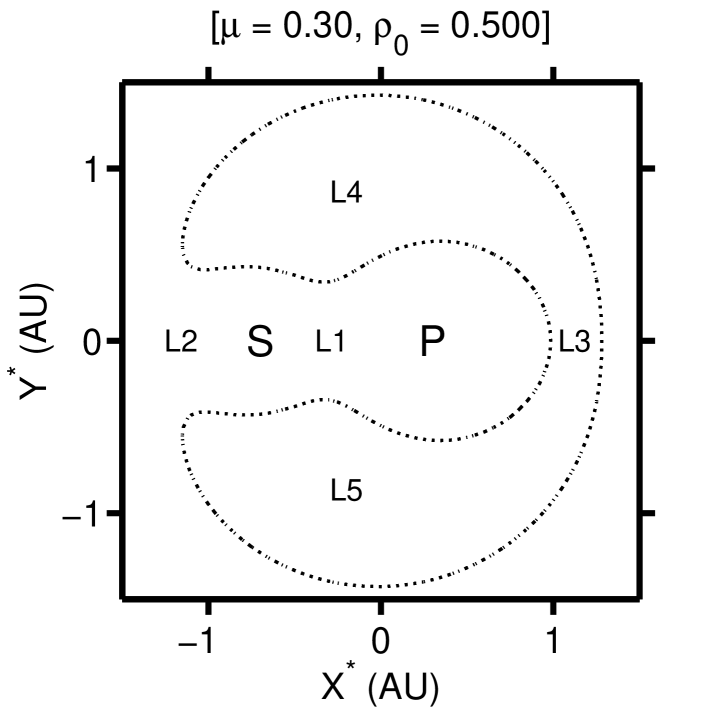
Figure 1: Locations of the Lagrange points L1, L2, L3, L4, and L5 as used in the CR3BP. The label P denotes the primary star and the label S denotes the secondary star.

Table 1: Errors in the Jacobi constant (JCE) for models of $\mu=0.3$ at different time intervals.

$\rho_{0}$	$\rm JCE({\tau\over 4})$	$\rm JCE({\tau\over 2})$	$\rm JCE({3\tau\over 4})$	$\rm JCE({\tau})$
0.355	1.0740E$-10$*	2.4747E$-10$*	1.2403E$-10$*	1.8824E$-10$*
0.474	1.4498E$-10$*	9.7917E$-11$*	3.7723E$-11$*	1.0067E$-11$*
0.595	8.9819E$-13$*	5.2923E$-13$*	5.2001E$-13$*	7.1001E$-06$*

• Note: $\tau$ denotes the runtime of the simulation. We show the stable cases of $\rho_{0}=0.355$ and 0.474 with $\tau=10^{5}$ binary orbits as well as the unstable case of $\rho_{0}=0.595$ with $\tau=150.64$ binary orbits.

Table 2: Maximum Lyapunov exponent study for the models of $\mu=0.3$ at different time intervals.

$\rho_{0}$	$\rm MLE\left({\rm 10^{2}}\right)$	$\rm MLE\left({\rm 10^{3}}\right)$	$\rm MLE\left({\rm 10^{4}}\right)$	$e_{\rm median}$	ZVC
0.20	1.1099E$-1$*	1.1493E$-2$*	1.1446E$-3$*	0.027	…
0.30	1.0322E$-1$*	1.0103E$-2$*	1.0691E$-3$*	0.17	…
0.40	9.8084E$-2$*	1.0050E$-2$*	6.8986E$-4$*	0.58	L1
0.474	7.7766E$-2$*	9.4232E$-3$*	9.2624E$-4$*	0.75	L1, L2
0.50	8.5390E$-2$*	9.2048E$-3$*	7.9830E$-4$*	0.85	L1, L2
0.595	1.5793E$-1$*	1.4175E$-1$*	…	1.14	L1, L2, L3
0.60	8.9533E$-1$*	…	…	1.10	L1, L2, L3

• Note: Elements without data indicate simulations that ended due to the energy criterion, thus representing planetary catastrophes. Elements with an asterisk (*) indicate that the simulation ended before the allotted time. Also, $e_{\rm median}$ represents the median of the eccentricity distribution obtained for the curvature of the planetary orbits in the synodic coordinate system (see Paper II). The last column indicates the Lagrange point(s) where the zero-velocity contour (ZVC) is open (see Paper I).

3 Results and discussion

We performed simulations for stellar mass ratios from $\mu=0.0$ to 0.5 in increments of 0.01. A Yoshida sixth order symplectic integration scheme was used (e.g., Yoshida 1990). As a measure of the precision of the integration scheme, we note that a time step of $\epsilon=10^{-4}$ yrs is used for the individual cases. However, for producing plots of the entire parameter space we adopt a time step of $\epsilon=10^{-3}$ yrs as the smaller time step did not noticeably enhance the quality of the plots. The order of error in energy for each time step was $10^{-14}$ and $10^{-10}$, respectively. We performed simulations for different time limits, which range from 10 to $10^{5}$ yrs in increments of powers of 10. We also performed case studies with time limits of $10^{6}$ and $10^{7}$ yrs, although we do not expect significant changes to occur at those longer time scales. By using different time scales we can estimate when certain phenomena occur and ascertain how they will affect other regions over longer periods of time.

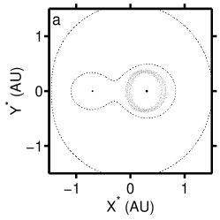
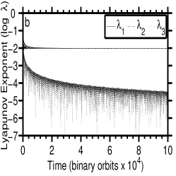
Figure 2: Case study for the initial planetary distance ratio $\rho_{0}=0.355$ with the planetary orbit in the synodic coordinate system, Lyapunov spectrum, and power spectrum. The stellar mass ratio is $\mu=0.3$.

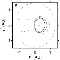
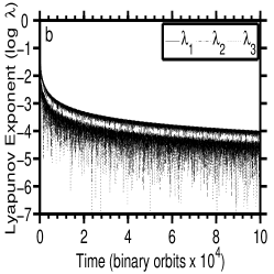
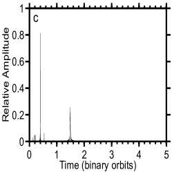
Figure 3: Case study for the initial planetary distance ratio $\rho_{0}=0.474$ with the planetary orbit in the synodic coordinate system, Lyapunov spectrum, and power spectrum. The stellar mass ratio is $\mu=0.3$.

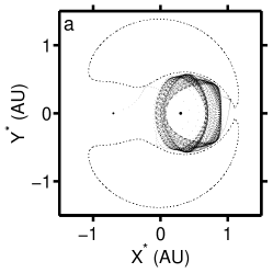
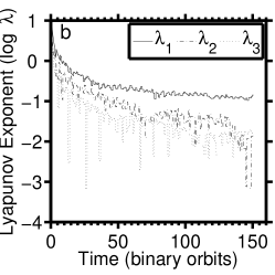
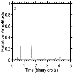
Figure 4: Case study for the initial planetary distance ratio $\rho_{0}=0.595$ with the planetary orbit in the synodic coordinate system, Lyapunov spectrum, and power spectrum. The stellar mass ratio is $\mu=0.3$.

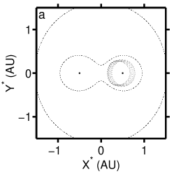
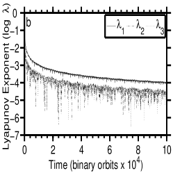
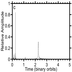
Figure 5: Case study for the initial planetary distance ratio $\rho_{0}=0.290$ with the planetary orbit in the synodic coordinate system, Lyapunov spectrum, and power spectrum. The stellar mass ratio is $\mu=0.5$.

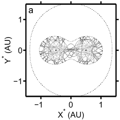
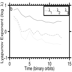
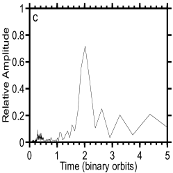
Figure 6: Case study for the initial planetary distance ratio $\rho_{0}=0.370$ with the planetary orbit in the synodic coordinate system, Lyapunov spectrum, and power spectrum. The stellar mass ratio is $\mu=0.5$.

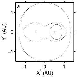
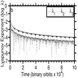
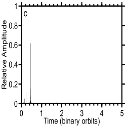
Figure 7: Case study for the initial planetary distance ratio $\rho_{0}=0.400$ with the planetary orbit in the synodic coordinate system, Lyapunov spectrum, and power spectrum. The stellar mass ratio is $\mu=0.5$.

We display runs for selected initial conditions (i.e., starting distances $\rho_{0}$ of the planet from the stellar primary) corresponding to $\mu=0.3$ in Figs. 2 to 4 and to $\mu=0.5$ in Figs. 5 to 7. In Figs. 2 to 7, we first present the planetary orbits in the synodic coordinate system (X*, Y*). Secondly in each figure, the Lyapunov spectra of the simulations are shown using a logarithmic scale for the Y*-axis. Lastly in each figure, the time series power spectra of the simulations are shown with their normalized amplitudes. The power spectra were obtained through the usage of a FFT subroutine in Matlab^® that uses the X*-component separation distance as a function of time and converts the output frequencies to periods. The selected starting distance ratios $\rho_{0}$ of the planet are 0.355, 0.474, 0.595 for $\mu=0.3$ and 0.290, 0.370, 0.400 for $\mu=0.5$. Note that $\rho_{0}$ indicates the relative initial distance of the planet given as $R_{0}/D$, with $D=1$ AU as the distance between the two stars and $R_{0}$ as the initial distance of the planet from its host star, the primary star of the binary system.

Using the method of Lyapunov exponents, we are able to verify and extend the methods described by Eberle et al. (2008) and Eberle & Cuntz (2010). Absolute orbital stability can be more rigorously shown through the Lyapunov exponent method. It occurs when $\rho_{0}<\rho_{0}^{\left(1\right)}$, where $\rho_{0}^{\left(1\right)}$ represents the point at which the initial condition results in a ZVC that opens at L1. For larger values of $\rho_{0}$, stability is not guaranteed due the behaviour discussed by Eberle et al. (2008); this result is also consistent with our Lyapunov exponent criterion for orbital stability.

Table 3: Maximum Lyapunov exponent study for the models of $\mu=0.5$ at different time intervals.

$\rho_{0}$	$\rm MLE\left({\rm 10^{2}}\right)$	$\rm MLE\left({\rm 10^{3}}\right)$	$\rm MLE\left({\rm 10^{4}}\right)$	$e_{\rm median}$	ZVC
0.25	8.7189E$-2$*	1.1353E$-2$*	1.0009E$-3$*	0.20	…
0.29	1.0647E$-1$*	9.5469E$-3$*	9.9141E$-4$*	0.45	L1
0.30	7.6275E$+0$*	…	…	0.67	L1
0.35	5.2937E$+0$*	…	…	0.82	L1
0.37	6.1946E$+0$*	…	…	0.98	L1
0.40	1.0675E$-1$*	9.6613E$-3$*	8.8900E$-4$*	0.71	L1
0.43	2.8614E$-1$*	2.9420E$-1$*	…	0.87	L1
0.50	7.9684E$-1$*	…	…	0.089	L1, L2, L3

• Note: Elements without data indicate simulations that ended due to the energy criterion, thus representing planetary catastrophes. Elements with an asterisk (*) indicate that the simulation ended before the allotted time. Also, $e_{\rm median}$ represents the median of the eccentricity distribution obtained for the curvature of the planetary orbits in the synodic coordinate system (see Paper II). The last column indicates the Lagrange point(s) where the zero-velocity contour (ZVC) is open (see Paper I).

In this paper, the main criterion for orbital stability is the Lyapunov exponent criterion, which is based on the maximum Lyapunov exponent. From a theoretical point of view, an orbit is stable when all Lyapunov exponents are exactly zero. Obviously, this ‘perfect’ criterion for orbital stability will be very difficult to reach numerically because it would require an infinite simulation time. Based on our finite simulation times, we obtain 3 positive and 3 negative Lyapunov exponents, and their sum becomes close to zero within the limits of our numerical simulations. Hence, in order to determine orbital stability numerically, we must look at the values of the three positive Lyapunov exponents at the beginning and at the end of our simulations. By comparing these values, we determine whether the exponents decrease in time, and if so what is the rate of their decrease, or whether they stay approximately constant in time.

Using this information, we are able to identify the maximum Lyapunov exponent and adopt it as our primary indicator of orbital stability. We classify an orbit as stable if the initial value of the maximum Lyapunov exponent is below a certain threshold and if it decreases at a ‘reasonable rate’ (see below); otherwise, the orbit is classified as unstable. In our plots of Lyapunov spectra (see the second panels in Figs. 2 to 7), we present all three positive Lyapunov exponents to show their values and study how they change in time.

In addition to the Lyapunov exponent criterion for orbital stability, we also use the so-called orbital energy criterion, which requires that the kinetic energy should not exceed twice the value of the potential energy. This is evaluated in our numerical simulations during each time step. A failure of this criterion would imply a break in conservation of the Jacobi constant as detailed by Szebehely (1967) and shown numerically in Table 1. It should also be noted that the cases presented in Table 1 are also presented in Figs. 2 to 4. There are two important points associated with this criterion. First, our systems are Hamiltonian, which means that their energy must be conserved. On the other hand, the fact that the energy conservation of the planet may be broken because we are neglecting the effects of the third mass on the larger masses has already been discussed by Szebehely (1967). Second, even if the energy is only approximately conserved in our numerical simulations, we still request that the Jacobi constant remains constant, which is a required stability condition for CR3BP. To be consistent with this criterion (see also Paper I), we stop our numerical simulation once changes (even small) in the Jacobi constant occur; such cases are depicted in Tables 2 and 3.

Alike in the previous paper by Eberle et al. (2008), we are able to identify the same regions of orbital stability, instability, and domains of quasi-periodic orbital stability. A key difference, however, is that the orbit diagrams depicted in Figs. 2 to 7 have been simulated for $10^{5}$ years, whereas the corresponding figures in the previous paper have been simulated for only $10^{3}$ years. The power spectra are shown to indicate how we determined the region of quasi-periodic orbital stability including the correct magnitude.

We begin by classifying Figs. 2, 3, 5, and 7 as stable candidate configurations. Three of the cases show similar behaviour in the maximum Lyapunov exponent as shown in Figs. 3b, 5b, and 7b. These Lyapunov spectra have a common trend by starting at a maximum value on the order of $10^{-1}$ and converging, albeit slowly, to smaller orders of ten. Figure 3 shows a somewhat different behaviour compared to the other cases in its class of stable candidates. This case establishes a quasi-periodic orbit, which illustrates a $\left(3:1\right)$ resonance in the power spectrum and reveals the same trend of stability in the Lyapunov exponent spectrum. Figure 2 shows an additional variance in behaviour due to the elevated nature of the maximum Lyapunov exponent. This shows that a limited amount of chaos exists in the system while remaining stable for the full simulation time. This case also demonstrates a $\left(4:1\right)$ resonance in the power spectrum.

In contrast, Fig. 4 demonstrates a case of instability. The Lyapunov spectrum shows a different nature than that of the preceding cases. In Fig. 4b it begins at a maximum value greater than 1 and converges to a value between $10^{-1}$ and 1. By establishing the preceding cases as stable cases, we can contrast the final values of the corresponding maximum Lyapunov exponents. In the unstable case of Fig. 4b, it is two orders of magnitude greater than in the stable cases of Figs. 3b, 5b, and 7b. However, in comparison with Fig. 2b we find only a difference of one order of magnitude.

Figure 6 has been examined in a similar manner. Having already classified Fig. 5 and 7 as stable configurations, we emphasize that they reveal similar trends in the maximum Lyapunov exponent as given by Fig. 3. However, Fig. 6 shows a different orbit diagram and is described by a maximum Lyapunov exponent that gives the outcome of instability. This case conveys a much noisier power spectrum along with a maximum Lyapunov exponent on the order of 1 or greater. Finer detail is illustrated in Table 1 and Table 2. Particularly Table 2 shows a boundary in the maximum Lyapunov exponent where values near 0.1 and smaller for the first 100 years tend toward stability.

Figure 8 conveys the bigger picture for the overall parameter space. It represents contour plots of the maximum Lyapunov exponent with respect to the ($\mu$, $\rho_{0}$) parameter space in linear and logarithmic scale. The crosses depict initial conditions for runs that prematurely ended due to the orbital energy criterion. This demonstrates where the regions of instability occur as reflected by the respective colour coded scale of the maximum Lyapunov exponent. Comparing Fig. 8 (left) to the previous result by Eberle et al. (2008), it can be seen that the main regions of stability remain the same. Other noteworthy features include that the instability islands present near $\rho_{0}=0.4$ have grown as the simulation time has been increased as well as the existence of a plateau near $\rho_{0}=0.48$. The colour scale in Fig. 8 (left) has a maximum colour of dark red at a maximum Lyapunov exponent of 0.15. Some regions appear to be coloured black; however, this does not correspond to the adopted colour scale as it is caused by the finite contour line width due to the close proximity of the lines. Therefore, the plateau has a peak value of a maximum Lyapunov exponent near 0.15. Considering the diagrams in Fig. 3, we conclude that a region of quasi-periodicity exists on this plateau.

Figure 8 (right), the contour plot in logarithmic scale, is shown to display some of the finer details pertaining to structure inside the stability regions. The blue-green coloured regions demonstrate areas of possible stable chaos that are hidden in Fig. 8 (left). Some other smaller contours are also produced in the stability region, but the colour coding in general shows little change, which is partially due to the chosen spacing between contours. The average difference in height between these levels is $-0.15$; on the logarithmic scale, it indicates a change by a factor of $1.41$ in the maximum Lyapunov exponent.

Inspecting Fig. 8 also allows a comparison with previous results, particularly results of Paper I. There it was shown that absolute orbital stability occurs when $\rho_{0}<\rho_{0}^{\left(1\right)}$, where $\rho_{0}^{\left(1\right)}$ represents the point at which due to the initial condition the ZVC opens at L1. This condition is represented by the line of C₁ in Fig. 8. It is evident that the Lyapunov exponent criterion is almost perfectly consistent with this condition. Additionally, as discussed in Paper I and references therein, no stability can be expected if $\rho_{0}>\rho_{0}^{\left(3\right)}$ because now the ZVC is open at L1, L2, and L3. This finding is also almost perfectly reflected through the behaviour of the maximum Lyapunov exponent as a orbital stability criterion. Both panels of Fig. 8 show no stability regions on the right side of C₃, which is reflective of the opening of the ZVC at Lagrange points L1, L2, and L3.

4 Conclusions

We present a detailed case study of the CR3BP with analyses through the usage of the Lyapunov exponents. We are able to characterize stability limits based on the value of the maximum Lyapunov exponent at the end of each simulation. Cases where the maximum Lyapunov exponent exceeds a value of 0.15 indicate that the planet will experience an event that causes the orbital velocity to decrease. These events include intersecting a Lagrange point or the ZVC. After such an event, the planet will experience a series of near misses (or collisions) with one of the stars in the binary system leading to overall instability. Chaos theory and the concept of Lyapunov time prevent us from predicting exactly when the planet will be ejected. Using the Lyapunov time as a measure of the length of predictive time, we can show that this relationship is proportional to the inverse of the maximum Lyapunov exponent. Using our critical value of 0.15, the unstable systems will lose predictability within $(0.15)^{-1}=6\frac{2}{3}$ years or less. After that time, it is unknown when the planet will be ejected as this could take many multiples of the Lyapunov time to occur.

The method also shows evidence of a region of quasi-periodicity. This is a region where the maximum Lyapunov exponent remains near the critical value without exceeding that value. This is shown for cases simulated for $10^{5}$ years. Based on this time scale, we can conclude that our quasi-periodic plateau represents a region of stable or quasi-stable chaos. This is due to the Lyapunov times being much less than the simulation run time. The chaos is shown through the value of the maximum Lyapunov exponent, whereas the stability is shown through the motion of the planet over longer time scales. The lack of near miss events and encounters with regions of decreasing velocity prohibits the planet from becoming orbitally unstable.

Comparisons to previously established criteria for stability show that our results are consistent with previously obtained stability limits (e.g., Holman & Wiegert 1999; Musielak et al. 2005; Cuntz et al. 2007; Eberle et al. 2008; Eberle & Cuntz 2010). In Eberle et al. (2008), Paper I, the onset of instability was related to the topology of the ZVC, whereas in Eberle & Cuntz (2010), Paper II, it was shown that the onset of orbital instability occurs when the median of the effective eccentricity distribution exceeds unity. Both results are consistent with the findings of Paper III, i.e., the inspection of the maximum Lyapunov exponent. However, the latter offers the advantage to link the study of orbital instability for the CR3BP (and any subsequent generalization, if available) to chaos theory, including the evaluation of different types of chaos.

Although our results have been obtained for the special case of the CR3BP, we expect that it may also be possible to augment our findings to planets in generalized stellar binary systems. Desired generalizations should include studies of the elliptical restricted 3-body problem (ER3BP) (e.g., Pilat-Lohinger & Dvorak 2002; Szenkovits & Makó 2008) as well as of planets on inclined orbits (Dvorak et al. 2007), noting that especially the former have important applications to real existing systems in consideration of the identified stellar and planetary orbital parameters (Eggenberger & Udry 2010).

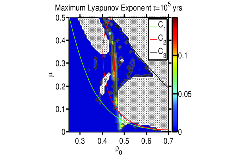
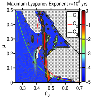
Figure 8: We depict the maximum Lyapunov exponent (colour coded) for various mass ratios $\mu$ and initial conditions $\rho_{0}$ using a linear scale (left) or a logarithmic scale (right) where $-n$ corresponds to $10^{-n}$. The crosses denote cases where the simulation was terminated due to the planet being captured by one of the stars or being ejected from the system. The green, red, and black curves represent the initial conditions that cause the ZVC to open at L1, L2, and L3, respectively.

Appendix A

Basic concepts and definitions

From stability analysis we can use a Jacobian matrix to show how a state vector x evolves in time (see Tsonis 1992 for details). The governing equations are

$$\dot{\textbf{x}}=\textbf{J}\cdot\textbf{x}$$

$$\textbf{J}=\left(\begin{array}[]{ccc}{\partial f_{1}\over\partial x_{1}}&\ldots&{\partial f_{n}\over\partial x_{1}}\\ \vdots&\ddots&\vdots\\ {\partial f_{1}\over\partial x_{n}}&\ldots&{\partial f_{n}\over\partial x_{n}}\end{array}\right)$$

This differential equation has a general solution, which is $\textbf{x}\left(t\right)=e^{\textbf{J}t}\>\textbf{x}\left(0\right)$. Assuming J has distinct eigenvalues, we can find a matrix U to diagonalize J to form a diagonal matrix D such as

$$\textit{U}^{-1}\>\textbf{J}\>\textit{U}=\textit{D}$$

By rewriting the above equation we obtain the more useful form given as

$$\textbf{J}=\textit{U}\>\textit{D}\>\textit{U}^{-1}$$

Using the multiplication theorem, we can develop relations to obtain the eigenvalues of J yielding

$$\det\>\textbf{J}=\left(\det\>\textit{U}\right)\left(\det\>\textit{D}\right)\left(\det\>\textit{U}^{-1}\right)=\det\>\textit{D}$$

$$=\lambda_{1}\lambda_{2}\cdots\lambda_{n}$$

Furthermore, we find

$$Tr\>\textbf{J}=Tr\>\textit{D}=\lambda_{1}+\lambda_{2}+\ldots+\lambda_{n}$$

This can be generalized from J to a function $f\left(\textbf{J}\right)$ such as

$$\det\>f\left(\textbf{J}\right)=f\left(\lambda_{1}\right)f\left(\lambda_{2}\right)\cdots f\left(\lambda_{n}\right)$$

$$Tr\>f\left(\textbf{J}\right)=f\left(\lambda_{1}\right)+f\left(\lambda_{2}\right)+\cdots+f\left(\lambda_{n}\right)$$

From our general solution, we can assume $f\left(\textbf{J}\right)=e^{\textbf{J}t}$. Therefore, we find

$$\det\>e^{\textbf{J}t}=e^{\left(\lambda_{1}+\lambda_{2}+\ldots+\lambda_{n}\right)t}=e^{\left(Tr\>\textbf{J}\right)t}$$

A volume of perturbations in phase space will be conserved if $\left|\det\>e^{\left(Tr\>\textbf{J}\right)t}\right|=1$ or $Tr\>\textbf{J}=0$ for Hamiltonian systems. A dissipative system will have $\left|\det\>e^{\left(Tr\>\textbf{J}\right)t}\right|<1$ or $Tr\>\textbf{J}<0$. The eigenvalues $\lambda_{1},\lambda_{2},\cdots,\lambda_{n}$ are the Lyapunov exponents of the flow or the logarithms of eigenvalues of J.

Numerical determination of Lyapunov exponents

From these equations we can define 6 dimensional tangent vectors $\textbf{x}_{i}$ and their derivatives $\dot{\textbf{x}}_{i}$ where $i=1,\ldots,6$ as

$$\textbf{x}_{i}=\left\{x_{i},y_{i},z_{i},u_{i},v_{i},w_{i}\right\}^{T}$$

$$\dot{\textbf{x}}_{i}=\left\{u_{i},v_{i},w_{i},\dot{u}_{i},\dot{v}_{i},\dot{w}_{i}\right\}^{T}$$

Also we can define a Jacobian matrix, J, given as

$$\textbf{J}=\left(\begin{array}[]{cccccc}0&0&0&1&0&0\\ 0&0&0&0&1&0\\ 0&0&0&0&0&1\\ {\partial\dot{u}\over\partial x}&{\partial\dot{u}\over\partial y}&{\partial\dot{u}\over\partial z}&0&2&0\\ {\partial\dot{v}\over\partial x}&{\partial\dot{v}\over\partial y}&{\partial\dot{v}\over\partial z}&-2&0&0\\ {\partial\dot{w}\over\partial x}&{\partial\dot{w}\over\partial y}&{\partial\dot{w}\over\partial z}&0&0&0\\ \end{array}\right)$$

Wolf method

Now we describe the scheme by which Wolf et al. (1985) determine the Lyapunov spectrum and its application to the CR3BP. The Wolf method follows a basic algorithm. The first step is to initialize a state vector of 6 elements. Then, the tangent vectors need to be initialized to some value. We choose to have all tangent vectors to be unit vectors for simplicity. This means that the elements $\left\{x_{1},\>y_{2},\>z_{3},\>u_{4},\>v_{5},\>w_{6}\right\}=1$ and all other elements will be equal to zero.

The next step consists of a loop that will use a standard integrator akin to the Runge-Kutta schemes to determine how the state and tangent vectors will change within a time step. This will continue for an adequate number of steps so that the tangent vectors become oriented along the flow. When this has been accomplished, it is necessary to perform a Gram-Schmidt Renormalization (GSR) to orthogonalize the tangent space. Thereafter, we take the logarithm of the length of each tangent vector to obtain the Lyapunov exponents. We then continue the loop.

Procedure

We use the first tangent vector, $\textbf{x}_{1}$, to define the basis for the GSR process. Thus, the first step consists in normalizing this vector. With the vectors of the new orthonormal set of tangent vectors, denoted by primes ($\prime$), we find

$$\begin{array}[]{l}\textbf{x}_{1}^{{}^{\prime}}={\textbf{x}_{1}\over\left\|\textbf{x}_{1}\right\|}\\ \textbf{x}_{2}^{{}^{\prime}}={\textbf{x}_{2}-\left\langle\textbf{x}_{2},\>\textbf{x}_{1}^{{}^{\prime}}\right\rangle\textbf{x}_{1}^{{}^{\prime}}\over\left\|\textbf{x}_{2}-\left\langle\textbf{x}_{2},\>\textbf{x}_{1}^{{}^{\prime}}\right\rangle\textbf{x}_{1}^{{}^{\prime}}\right\|}\\ \vdots\\ \textbf{x}_{6}^{{}^{\prime}}={\textbf{x}_{6}-\left\langle\textbf{x}_{6},\>\textbf{x}_{5}^{{}^{\prime}}\right\rangle\textbf{x}_{5}^{{}^{\prime}}-\ldots-\left\langle\textbf{x}_{6},\>\textbf{x}_{1}^{{}^{\prime}}\right\rangle\textbf{x}_{1}^{{}^{\prime}}\over\left\|\textbf{x}_{6}-\left\langle\textbf{x}_{6},\>\textbf{x}_{5}^{{}^{\prime}}\right\rangle\textbf{x}_{5}^{{}^{\prime}}-\ldots-\left\langle\textbf{x}_{6},\>\textbf{x}_{1}^{{}^{\prime}}\right\rangle\textbf{x}_{1}^{{}^{\prime}}\right\|}\\ \end{array}$$

From this new set of tangent vectors, the Lyapunov exponents will be calculated considering the lengths of each vector. Therefore, we find

$$\lambda_{i}={1\over\tau}\left[\lambda_{i-1}+\log\left\|\textbf{x}_{i}-\sum_{j=1}^{i}{\left\langle\textbf{x}_{i},\>\textbf{x}_{j-1}^{{}^{\prime}}\right\rangle\textbf{x}_{j-1}^{{}^{\prime}}}\right\|\right]$$

$\ \rm where\>\lambda_{o}=\textbf{x}_{o}^{{}^{\prime}}=0$.

References

- Baker & Gollub (1990) Baker, G. L., & Gollub, J. P. 1990, Chaotic Dynamics: An Introduction (Cambridge: Cambridge University Press)
- Benettin et al. (1980) Benettin, G., Galgani, L., Giorgilli, A., & Strelcyn, J.-M. 1980, Meccanica, 15, 9
- Catanzarite et al. (2006) Catanzarite, J., Shao, M., Tanner, A., Unwin, S., & Yu, J. 2006, PASP, 118, 1319
- Cockell et al. (2009) Cockell, C. S., Léger, A., Fridlund, M., et al. 2009, Astrobiology, 9, 1
- Cuntz et al. (2007) Cuntz, M., Eberle, J., & Musielak, Z. E. 2007, ApJ, 669, L105
- Duquennoy & Mayor (1991) Duquennoy, A., & Mayor, M. 1991, A&A, 248, 485
- Dvorak (1984) Dvorak, R. 1984, Celest. Mech. Dyn. Astron., 34, 369
- Dvorak (1986) Dvorak, R. 1986, A&A, 167, 379
- Dvorak et al. (2007) Dvorak, R., Schwarz, R., Sűli, Á., & Kotoulas, T. 2007, MNRAS, 382, 1324
- Eberle & Cuntz (2010) Eberle, J., & Cuntz, M. 2010, A&A, 514, A19 (Paper II)
- Eberle et al. (2008) Eberle, J., Cuntz, M., & Musielak, Z. E. 2008, A&A, 489, 1329 (Paper I)
- Eggenberger & Udry (2010) Eggenberger, A., & Udry, S. 2010, in Planets in Binary Star Systems, ed. N. Haghighipour (New York: Springer), 19
- Eggenberger et al. (2004) Eggenberger, A., Udry, S., & Mayor, M. 2004, A&A, 417, 353
- Fouchard et al. (2002) Fouchard, M., Lega, E., Froeschlé, Ch., & Froeschlé, Cl. 2002, Cel. Mech. Dyn. Astron., 83, 205
- Froeschlé et al. (1997) Froeschlé, C., Lega, E., & Gonczi, R. 1997, Cel. Mech. Dyn. Astron., 67, 41
- Gonczi & Froeschlé (1981) Gonczi, R., & Froeschlé, C. 1981, Cel. Mech. Dyn. Astron., 25, 271
- Hilborn (1994) Hilborn, R. C. 1994, Chaos and Nonlinear Dynamics (Oxford: Oxford University Press)
- Holman & Wiegert (1999) Holman, M. J., & Wiegert, P. A. 1999, AJ, 117, 621
- Jefferys & Yi (1983) Jefferys, W. H., & Yi, Z.-H. 1983, Cel. Mech. Dyn. Astron., 30, 85
- Lada (2006) Lada, C. J. 2006, ApJ, 640, L63
- Lecar et al. (1992) Lecar, M., Franklin, F., & Murison, M. 1992, AJ, 104, 1230
- Lissauer (1999) Lissauer, J. J. 1999, Rev. Mod. Phys., 71, 835
- Lyapunov (1907) Lyapunov, M. A. 1907, Ann. Fac. Sci., University of Toulouse, 9, 203
- Malhotra (1998) Malhotra, R. 1998, in Solar System Formation and Evolution, ed. D. Lazzaro, R. Vieira Martins, S. Ferraz-Mello, & J. Fernandez (San Francisco: ASP), 149, 37
- Mardling (2007) Mardling, R. A. 2007, in Dynamical Evolution of Dense Stellar Systems, ed. E. Vesperini, M. Giersz, & A. Sills, Proc. IAU Symp. 246, 199
- Milani & Nobili (1992) Milani, A., & Nobili, A. M. 1992, Nature, 357, 569
- Murray & Holman (2001) Murray, N., & Holman, M. 2001, Nature, 410, 773
- Musielak et al. (2005) Musielak, Z. E., Cuntz, M., Marshall, E. A., & Stuit, T. D. 2005, A&A, 434, 355; Erratum, 480, 573 [2008]
- Musielak & Musielak (2009) Musielak, Z. E., & Musielak, D. E. 2009, Int. J. Bifurcation and Chaos, 19, 2823
- Ozorio de Almeida (1990) Ozorio de Almeida, A. M. 1990, Hamiltonian Systems: Chaos and Quantization (Cambridge: Cambridge University Press)
- Patience et al. (2002) Patience, J., White, R. J., Ghez, A. M., et al. 2002, ApJ, 581, 654
- Pilat-Lohinger & Dvorak (2002) Pilat-Lohinger, E., & Dvorak, R. 2002, Celest. Mech. Dyn. Astron., 82, 143
- Rabl & Dvorak (1988) Rabl, G., & Dvorak, R. 1988, A&A, 191, 385
- Raghavan et al. (2006) Raghavan, D., Henry, T. J., Mason, B. D., et al. 2006, ApJ, 646, 523
- Roy (2005) Roy, A. E. 2005, Orbital Motion (Bristol and Philadelphia: Institute of Physics Publ.)
- Smith & Szebehely (1993) Smith, R. H., & Szebehely, V. 1993, Celest. Mech. Dyn. Astron., 56, 409
- Szebehely (1967) Szebehely, V. 1967, Theory of Orbits (New York and London: Academic Press)
- Szenkovits & Makó (2008) Szenkovits, F., & Makó, Z. 2008, Celest. Mech. Dyn. Astron., 101, 273
- Tsonis (1992) Tsonis, A. A. 1992, Chaos. From Theory to Applications (New York: Plenum Press)
- Yoshida (1990) Yoshida, H. 1990 Phys. Lett. A, 150, 262
- Wolf et al. (1985) Wolf, A., Swift, J. B., Swinney, H. L., & Vastano, J. A. 1985, Physica D, 16, 285