A Forward Branching Phase-Space Generator

Abstract

We develop a forward branching phase-space generator for use in next-to-leading order parton level event generators. By performing $2\to 3$ branchings from a fixed jet phase-space point, all bremsstrahlung events contributing to the given jet configuration are generated. The resulting phase-space integration is three-dimensional irrespective of the considered jet multiplicity. In this first study, we use the forward branching phase-space generator to calculate in the leading-color approximation next-to-leading order corrections to fully differential gluonic jet configurations.

1 Introduction

The evaluation of the virtual corrections to processes including a large number of jets has become straightforward [1, 2, 3, 4, 5, 6, 7, 8, 9, 10, 11, 12, 13, 14, 15, 16, 17, 18, 19] due to the advent of algorithmic implementations [20, 21, 22, 23, 24, 25, 26, 27] of generalized unitarity [28, 29] using parametric integration techniques [30]. The only required diagrammatic evaluations are partonic tree-level amplitudes. These diagrams can be efficiently evaluated through algorithmic recursion relations [31, 32, 33, 34, 35, 36, 37, 38, 39, 40, 41, 42]. As a consequence, all building blocks exist to construct a Next-to-Leading Order (NLO) event generator for the evaluation of high multiplicity jet observables. Such a generator would expand the possible phenomenological studies at, for example, the Large Hadron Collider (LHC) significantly.

However, the integration of the bremsstrahlung events over phase space hinders further development of such generators. Current methods for the automated numerical integration [43, 44, 45, 46, 47, 48, 49, 50] of the real matrix elements over the high dimensional phase space require large computer resources. Already for $2\to 4$ processes, the obtainable statistical accuracy is a limiting factor for realistic phenomenology.

On the other hand, shower Monte Carlo programs [51, 52, 53, 54, 55, 56, 57] tell us efficient algorithms exist to generate events closely following the physics [58]. It is therefore of interest to investigate phase-space generators based on especially dipole showers [59, 60, 61, 62, 63, 64, 65, 66] as they employ exact phase-space factorization. A shower based NLO phase-space generator uses as a starting point an $n$-parton final state, which can have additional multiple non-partonic particles. The origin of this final state does not affect the NLO generator. It can be a previously generated Leading Order (LO) event (weighted or unweighted), an event provided by a phase-space generator such as Rambo [67], Sarge [68], Haag [69], Kaleu [70] or any other source. The Forward Branching Phase-Space (FBPS) generator will interpret each of the $n$ parton momenta as a jet momentum. Next, following the dipole shower formalism, it performs forward $2\to 3$ branchings, thereby generating the $(n+1)$-parton phase space. The brancher is constructed in a way that a jet algorithm based on a $3\to 2$ clustering algorithm exactly inverts the branching. As a consequence the observed final state is unaltered during the phase-space integration.

As a result, any observable constructed from the fixed number of jet momenta remains unaltered by the FBPS generator and hence does not constrain the real-emission phase-space integration, which can thus be viewed as integrating out the partonic degrees of freedom inside the jets. In this sense the jet has become opaque and no information can be extracted about the internal jet structure, which is the domain of resummed calculations, in particular parton showers. We note that if a dipole shower would use the same brancher, the matching of this shower to the NLO calculation becomes a triviality as the shower, just as the observables, factorizes from the bremsstrahlung integration. In other words, the shower does not alter the NLO event weight nor does it change the partonic jet observable.

The FBPS generator is an one-particle phase-space integrator, independent from the number of jets. Therefore, for a given $n$-jet configuration, the numerical accuracy is only affected by the number of possible $2\to 3$ branchings, i.e. the number of jet pairs. This means that in order to maintain constant statistical accuracy, as the number of jets increase, the Monte Carlo program needs $\mathcal{O}(N_{\mathrm{evts}}\times n^{2})$ generated bremsstrahlung events where $N_{\mathrm{evts}}$ is a number of events independent of the jet multiplicity $n$. An additional virtue is that all generated bremsstrahlung events are added to the same virtual event, making the infra-red/collinear cancellations efficient and easy to optimize in the three-dimensional phase space. This allows us to use a simple slicing method to facilitate the cancellation of the infra-red/collinear singularities. Note that subtraction methods can be trivially implemented as any jet observable does not depend on the generated bremsstrahlung event.

In the first implementation of this method, we use a special $3\rightarrow 2$ clustering jet algorithm, which is an augmented $2\rightarrow 1$ jet algorithm. This augmentation adds a recoil parton to the $2\rightarrow 1$ clustering. As a result, the NLO jet phase space becomes identical to the LO jet phase space. Specifically, jets resulting from the clustering remain massless and the jet algorithm preserves momentum conservation, i.e. particles “clustered” with the beam are not discarded. From these observations it is clear, the jet augmentations will only modify the last step in the jet algorithm: the clustering prescription. The clustering step is added rather ad-hoc to current jet algorithms, which makes it easier to implement the necessary modifications as described later on in this paper.

The layout of the paper is as follows. In Section 2 we discuss issues regarding the infra-red safety of jet observables. We will propose augmentations of the jet algorithms to make all possible jet observables infra-red safe. Because of their enhanced infra-red safe behavior, these augmented jet algorithms have improved theoretical properties. We will use these properties to construct the FBPS generator in Section 3. With this phase-space generator at hand, we build – as a proof-of-principle – a leading-color NLO parton level event generator for $PP\to n$ gluonic jets. This is detailed in Section 4, before we give our conclusions in Section 5. Finally, two appendices are added. The first appendix details the number and type of branchings occurring in the FBPS generator. The second appendix lists the explicit jet configurations utilized in Section 4 to perform the numerical studies.

2 The Fully Differential Jet Cross Section

At hadron colliders, jets form the basis of defining the event topology and thereby characterize the underlying hard scattering event. It is therefore imperative to understand jets in both experiment and theory. An essential requirement of the jet defining algorithm is infra-red finiteness, which expresses the fact that the addition of arbitrary soft/collinear particles does not alter the final-state jet multiplicity. The infra-red finiteness requirement in jet algorithms is by now well understood (see e.g.  [71]).

Before the advent of the numerical parton level NLO generators [72, 73], semi-numerical programs calculated corrections to differential jet observables. For example, in Ref. [74] the NLO corrections to the semi-exclusive dijet cross section are calculated for explicitly given values of the dijet mass and the rapidities of the two leading jets. This gives a necessarily infra-red safe (finite) correction for each point in the dijet phase space. Note that the jet algorithm inevitably forms an integral part of this calculation.

Current parton level NLO multi-jet generators perform a Monte Carlo integration over the bremsstrahlung phase space independently of any actual jet algorithm. This has the apparent advantage that any experimental jet algorithm can be numerically accommodated in the Monte Carlo programs. However, owing to the infra-red properties of the jet algorithms, the generators only produce infra-red safe results for more inclusive jet observables. The resulting predictions from the Monte Carlo generators are not infra-red safe for each point in the multi-jet phase space as the LO and NLO jet phase spaces only coincide on the boundary defined by soft/collinear emissions. A sufficient amount of jet phase-space averaging is required to obtain finite results. For example, one cannot use arbitrarily small bin sizes in representing the results of the Monte Carlo integration – sufficiently wide bins are needed.

As mentioned above while current jet algorithms are infra-red finite, the observables constructed from these jets are not necessarily infra-red safe. This is a direct consequence of the clustering procedure constituting the last step of the jet algorithms. For example, the dijet azimuthal angle de-correlation is a typical non infra-red safe jet observable [75, 76]. At LO ($n=2$), the two jets in the event are exactly back-to-back in the azimuthal plane. At NLO, the generation of the jet mass will cause the bremsstrahlung events to deviate from the back-to-back configuration leaving uncanceled logarithmic divergences. On the contrary, with an infra-red safe jet algorithm, the NLO jet phase space is identical to the LO jet phase space and the two jets remain balanced. All that is calculated at NLO is the $K$-factor; only a third jet will induce a de-correlation.

It is important to note that the Kinoshita–Lee–Nauenberg (KLN) theorem is not a jet phase-space averaged property. By integrating over all partonic contributions to a fixed jet configuration, the KLN theorem should already hold. In other words, an infra-red safe jet algorithm must provide a proper cancellation between virtual and bremsstrahlung events for each jet phase-space point. As a consequence any jet observable constructed through an infra-red safe jet algorithm is finite.

2.1 Jet algorithms and infra-red safe observables

To explore the issues with jet algorithms further, we will first look at final-state jets at a lepton collider: $\ell^{+}\ell^{-}\to J_{1}\cdots J_{n}$. Here, a sequential jet algorithm is readily constructed by defining, as a function of the cluster momenta $\{c_{i}\}$, an event resolution measure $R_{\mathrm{evt}}(c_{1},\ldots,c_{m})$. The event resolution separates the soft/collinear region from the hard region of phase space. The clusters can be individual hadrons, calorimeter cells, tracks and combinations thereof. If $R_{\mathrm{evt}}$ is smaller than the requested jet resolution, $R_{\mathrm{jet}}$, the number of clusters is recombined using the cluster procedure defined by the specific jet algorithm: $\{c_{1},\ldots,c_{m}\}\mapsto\{\hat{c}_{1},\ldots,\hat{c}_{m-1}\}$. This is repeated until $R_{\mathrm{evt}}\geq R_{\mathrm{jet}}$, at which point the remaining clusters are identified as the jets.

Jet algorithms currently used by experiments ([77, 78, 79, 80, 81, 71]) define the event resolution function in terms of resolution functions of pairs of clusters: $R_{\mathrm{evt}}=\min_{ij}R_{ij}:R_{ij}=R(c_{i},c_{j})$. The minimization procedure identifies the least resolved pair of clusters and recombines these two clusters to one new cluster, thereby decreasing the total number of clusters in the event by one. In here lies a fundamental issue: either the newly formed cluster has a four-momentum, which is massive due to adding the momenta of the two clusters $\hat{c}_{ij}=c_{i}+c_{j}$, or overall momentum conservation is violated. From a theoretical point of view, the $2\to 1$ clustering causes the NLO jet phase space to separate from the LO jet phase space. The LO jets are massless, while the NLO jets now necessarily are massive. They only match in the exact soft/collinear limit, in which case the new cluster is massless: $\hat{c}_{ij}=0$. As a result we have infra-red finiteness, but no infra-red safety. The necessary care has to be taken when defining jet observables. For a given value of a jet observable ${\mathcal{O}}_{\mathrm{obs}}$, the virtual correction contributes at a single point $\delta({\mathcal{O}}-{\mathcal{O}}_{\mathrm{obs}})$ while, because of the jet mass, the bremsstrahlung is distributed as $\log({\mathcal{O}}-{\mathcal{O}}_{\mathrm{obs}})$. This behavior is “cured” by allowing, for example, sufficient smearing in histogram bins.

To maintain infra-red safety, we need to both keep massless clusters and maintain overall momentum conservation when combining clusters. The minimal procedure to do this is by defining the resolution function in terms of triplets of clusters [82]: $R_{\mathrm{evt}}=\min_{ijk}R(c_{i},c_{j},c_{k})$. The triplets of clusters $\{c_{i},c_{j},c_{k}\}$ can be recombined to pairs of clusters $\{\hat{c}_{i},\hat{c}_{j}\}$, while maintaining both momentum conservation, $\hat{c}_{i}+\hat{c}_{j}=c_{i}+c_{j}+c_{k}$, and keeping the newly formed clusters massless, $\hat{c}_{i}^{2}=\hat{c}_{j}^{2}=0$. With this type of jet algorithm one can define infra-red safe jet cross sections. As a consequence the fully differential cross section $d^{(n)}\sigma/d\,J_{1}\cdots d\,J_{n}$, and all possible distributions of jet observables derived from it, are infra-red safe. The reason this can be done is that the LO and NLO jet phase spaces exactly match. We can therefore construct a phase-space brancher similar to the ones used in dipole showers [61, 64]. By choosing the branching map as the inverse of the $3\to 2$ clustering used in the jet algorithm, all generated bremsstrahlung events are mapped back to the same jet phase-space point. This results in an infra-red safe, fully differential jet cross section by virtue of the KLN theorem. That is, both virtual and bremsstrahlung corrections contribute to $\delta({\mathcal{O}}-{\mathcal{O}}_{\mathrm{obs}})$ only and no smearing is required to obtain a finite result.

As is clear from the above discussions, it is straightforward to construct a FBPS generator for lepton colliders. It would calculate the $K$-factor to a fixed jet phase-space point, i.e. the fully differential jet cross section. However, for hadron colliders, the incoming partons cause additional complications. The current jet algorithms used in hadron colliders augment the lepton collider jet algorithms by including a resolution measure of clusters with respect to the beam. If a cluster is combined with the beam, it is effectively removed. As a result the remaining clusters violate momentum conservation as we have un-clustered momenta. To get infra-red safety, momentum conservation must be preserved during the clustering. There are two options: either build up a beam jet, or perform final-state clusterings only.

The first option is to construct a beam jet: instead of removing the final-state clusters, when combining with the incoming beam, they are combined with the respective (separate) beam cluster. Once the event resolution passes the jet resolution, we are left with two incoming beam jets and the final-state jets. All jets are massless and four-momentum is conserved. However, the two beam-jet momenta are not along the incoming (anti-)proton directions. To map onto the LO jet phase space, where the two beam-jet momenta are along the incoming (anti-)proton directions, we have to define the jet observables in the frame where the two beam jets are along the (anti-)proton directions. That is, we have to perform a transverse momentum boost to this frame. From a theoretical point of view, this has the desirable feature that the effect of “initial-state radiation” is minimized as this radiation does not affect the observable due to the boost. Effectively, the initial-state radiation is integrated out within the jet cone and the KLN theorem guarantees a properly defined fully differential jet cross section.

The second option is to constrain the initial-state clusters to remain along the respective beam direction during the clustering phase: the beam particle momenta are only rescaled. While not immediately obvious, this can always be accomplished using the $3\to 2$ clustering maps. From an experimental point of view, this is not a particular desirable option as all radiation is assigned to the final-state jets.

For a proof-of-principle calculation, the second option is highly desirable as it minimizes theoretical complications. It will be used in this paper. As this is a NLO calculation, only one clustering step is performed. We start with the partonic scattering $p_{a}\,\!p_{b}\to p_{1}\cdots p_{n+1}$ and reduce this to the jet final state $J_{a}\,\!J_{b}\to J_{1}\cdots J_{n}$. Note that $a$ and $b$ are only used to label the incoming partons or jets; no flavor information is associated with these labels. Out of the large class of infra-red safe jet algorithms, which can be constructed, the explicit jet algorithm used in this paper is as follows:

1. Find initial- or final-state parton $i$ and final-state parton $j$ by minimizing the resolution parameter

   $$R_{ij}\;=\;|\,\!s_{ij}|\,=\,\left|(\pm p_{i}+p_{j})^{2}\right|$$ (1)

   where “$+$” is used for $i$ being a final-state particle and “$-$” for being an initial-state particle.

2. Given partons $i$ and $j$ of the previous step, find final-state parton $k$ by minimizing

   $$R_{ij;k}\;=\;\min\left(R_{ik},R_{jk}\right)\ .$$ (2)

3. If parton $i$ is a final-state parton: cluster parton $i$ and $j$, $p_{ij}=p_{i}+p_{j}$, and use parton $k$ as the recoil momentum to make the cluster massless:

   $$\left\{\begin{array}[]{l}J_{i}\;=\;p_{ij}+(1-\gamma)\,p_{k}\ ,\\[5.69054pt] J_{k}\;=\;\gamma\,p_{k}\end{array}\right.$$ (3)

   with $\gamma=1+s_{ij}/(s_{ik}+s_{jk})$. This maps the three final-state partons onto two massless jets: $\{p_{i},p_{j},p_{k}\}\mapsto\{J_{i},J_{k}\}$ while preserving momentum conservation: $J_{i}+J_{k}=p_{i}+p_{j}+p_{k}$.

4. If parton $i$ is an initial-state parton, say $i=a$: cluster the two final-state momenta, $p_{jk}=p_{j}+p_{k}$, and use the initial-state parton $a$ as the recoil momentum to make the cluster massless:

   $$\left\{\begin{array}[]{l}J_{a}\;=\;\gamma\,p_{a}\ ,\\[5.69054pt] J_{j}\;=\;p_{jk}-(1-\gamma)\,p_{a}\end{array}\right.$$ (4)

   with $\gamma=1-s_{jk}/(s_{aj}+s_{ak})$. The two final-state partons are now mapped onto one massless jet and a rescaled initial-state parton: $\{p_{a},p_{j},p_{k}\}\mapsto\{J_{a},J_{j}\}$, while maintaining overall momentum conservation $J_{a}-J_{j}=p_{a}-p_{j}-p_{k}$.

We will use an inclusive mode of the algorithm. This means, we keep clustering until the desired (LO predefined) number of jets is reached. The alternative is to cluster until the jet resolution exceeds the preset minimum, after which the event is vetoed, if the number of jets is not equal to the desired number of jets. This is the exclusive mode of the algorithm, which is not used in this paper. Note that for reproducing the usual NLO $n$-jet inclusive observables, we have to perform a two-stage run. First, generate the NLO $K$-factors for the exclusive $n$-jet events, next, add the $(n+1)$-jet events at LO. From this event sample the observable can be determined.

2.2 Defining the fully differential jet cross section

We want to calculate the fully differential cross section of an $n$-jet final state characterized by the jet-axis momenta $J_{1},\ldots,J_{n}$ using the inclusive version of the jet algorithm specified in the previous subsection. The jet event kinematics are given by

$$x_{a}\,P_{a}+x_{b}\,P_{b} = J_{1}+\cdots+J_{n}\ ,$$ (5)

$$J_{i}^{2} = 0\ ,$$

where $P_{a,b}$ denote the incoming hadron momenta and

$$x_{a,b}\,P_{a,b}\;=\;x_{a,b}\,\frac{\sqrt{S}}{2}\,(1,\pm 1,0,0)\ .$$ (6)

The collider energy is given by $\sqrt{S}$ and the momentum fractions $x_{a}$ and $x_{b}$ are calculated from the reconstructed jets:

$$x_{a,b}\;=\;\frac{1}{\sqrt{S}}\;\sum_{i=1}^{n}\,p_{T}^{(i)}\,e^{\pm y_{i}}\ ,$$ (7)

using the transverse momenta and rapidities of the jets,

$$p_{T}^{(i)}\;=\;\sqrt{(p_{x}^{(i)})^{2}+(p_{y}^{(i)})^{2}}\qquad\quad\mbox{and}\qquad\quad y_{i}\;=\;\frac{1}{2}\,\log\left(\frac{E^{(i)}+p_{z}^{(i)}}{E^{(i)}-p_{z}^{(i)}}\right)\ ,$$ (8)

respectively. Note that here we have used the convention $p=(E,p_{z},p_{x},p_{y})$.

We define the differential cross section of the jet observable ${\mathcal{O}}$ as

$$\frac{d\,\sigma}{d\,{\mathcal{O}}}\;=\;\frac{1}{n!}\,\!\int d\,\Phi\big{(}x_{a}P_{a},x_{b}P_{b}\mapsto J_{1},\ldots,J_{n}\big{)}\ d\,x_{a}\,d\,x_{b}\ \delta\Big{(}{\mathcal{O}}-{\mathcal{O}}\big{(}J_{1},\ldots,J_{n}\big{)}\Big{)}\ \frac{d^{(n)}\sigma}{d\,J_{1}\cdots d\,J_{n}}\ ,$$ (9)

where the jet phase space is given by

$$d\,\Phi\big{(}x_{a}P_{a},x_{b}P_{b}\mapsto J_{1},\ldots,J_{n}\big{)} = \left(\prod_{i=1}^{n}d^{(4)}J_{i}\ \delta(J_{i}^{2})\ \theta(E_{i})\right)\delta(x_{a}P_{a}+x_{b}P_{b}-J_{1}-\cdots-J_{n})$$ (10)

$$= \left(\prod_{i=1}^{n}\frac{d^{(3)}\vec{J_{i}}}{2\,E_{i}}\right)\delta(x_{a}P_{a}+x_{b}P_{b}-J_{1}-\cdots-J_{n})\ .$$

We consider all jets as indistinguishable and hence have to introduce the “identical-jets” averaging factor of $(n!)^{-1}$. The fully differential jet cross section at LO is given by

$$\frac{d^{(n)}\sigma_{\textrm{\tiny LO}}}{d\,J_{1}\cdots d\,J_{n}}\;=\;\frac{(2\pi)^{4-3n}}{2\,x_{a}x_{b}\,S}\ \sum_{\{f_{a}f_{b}\to f_{1}\cdots f_{n}\}}F_{f_{a}}(x_{a})\,F_{f_{b}}(x_{b})\ \left|\overline{\mathcal{M}}^{(0)}\big{(}x_{a}P_{a},x_{b}P_{b};J_{1},\ldots,J_{n}\big{)}\right|^{2}\ ,$$ (11)

where the $F_{f_{a,b}}$ are the parton density functions of the partons in the beam particles and $\big{|}\,\overline{\mathcal{M}}^{(0)}\big{|}^{2}$ is the squared LO scattering amplitude, spin/color summed (averaged) over final (initial) states. The flavor sum runs over all possible, distinguishable partonic subprocesses $f_{a}f_{b}\to f_{1}\cdots f_{n}$ that contribute to the jet final state. For example, a $q\bar{q}+(n-2)g$ final state has $n(n-1)$ distinct flavor terms to be added for one specific initial-state configuration. This way we account for all ways of assigning the distinguishable partons of the final state $f_{1},\ldots,f_{n}$ to the jets $J_{1},\ldots,J_{n}$. Note that at LO no phase-space integration is left for the fully differential jet cross section. However, using our definition, the fully differential jet cross section will be symmetric under any exchange of partons without the need of integrating over phase space. Once one does the phase-space integration, as in Eq. (9), the usual symmetry factors are recovered.

Because the jet algorithm preserves explicit momentum conservation and keeps the jets massless, we can define a $K$-factor per jet phase-space point $J_{1},\ldots,J_{n}$. The NLO corrections to the fully differential jet cross section can hence be written as

$$\frac{d^{(n)}\sigma_{\textrm{\tiny NLO}}}{d\,J_{1}\cdots d\,J_{n}}\;=\;K_{\textrm{\tiny NLO}}\big{(}J_{1},\ldots,J_{n}\big{)}\;\times\;\frac{d^{(n)}\sigma_{\textrm{\tiny LO}}}{d\,J_{1}\cdots d\,J_{n}}\ .$$ (12)

In the remainder of the paper we will derive the expression for $K_{\textrm{\tiny NLO}}$ and develop, as a proof-of-principle, a Monte Carlo integrator for the explicit evaluation of the $K$-factor for the pure gluonic contribution of an $n$-jet event at a hadron collider. The $K$-factor is composed of three contributions, the Born contribution expressed as “1”, the virtual contribution, $V$, and the bremsstrahlung part, $R$. We write

$$K_{\textrm{\tiny NLO}}\big{(}J_{1},\ldots,J_{n}\big{)} = 1\;+\;\widetilde{V}\big{(}J_{1},\ldots,J_{n}\big{)}\;+\;\widetilde{R}\big{(}J_{1},\ldots,J_{n}\big{)}$$ (13)

$$= 1\;+\;\left(\frac{\alpha_{S}N_{\mathrm{C}}}{2\pi}\right)\Big{(}V(J_{1},\ldots,J_{n})\;+\;R(J_{1},\ldots,J_{n})\Big{)}\ ,$$

where we have factorized the strong-coupling expansion parameter $\alpha_{S}/2\pi$ and the color factor $N_{\mathrm{C}}$. Eq. (13) expresses the cancellation of infra-red singularities per jet phase-space point, $\widetilde{V}$ and $\widetilde{R}$ on their own diverge but their sum gives a finite contribution to the $K$-factor. For the calculation of the virtual corrections, many packages have been developed [22, 1, 2, 3, 4, 5, 6, 24, 7, 8, 9, 10, 25, 16, 26], which can be readily used to calculate this part of the $K$-factor. On the other hand, the calculation of the bremsstrahlung contribution $R$ requires a careful derivation.

To summarize, for the calculation of a jet observable, we generate, using Eq. (9), the jet configurations contributing to the specific value of the observable. For each generated jet phase-space point, we calculate the LO weight according to Eq. (11) and the NLO re-weighting multiplicative $K$-factor as given in Eq. (12).

3 The Forward Branching Phase-Space Generator

The explicit construction of the FBPS generator proceeds in several steps. In Section 3.1 the first step is taken by the decomposition of the bremsstrahlung phase space into sectors using the event resolution function given by the jet algorithm. Each sector is defined through the jet algorithm selecting an unique triplet of partons to be clustered. Next, owing to the invertibility of the clustering, we develop in Section 3.2 the real-emission phase-space formalism based on forward branching off the Born level jet configurations. In Section 3.3, we derive the specific forward branchers, which fill each sector such that the $3\to 2$ cluster map given by the jet algorithm will recombine the three partons to the same two jets specified by the jet phase-space point. Finally, in Section 3.4, the procedure is validated using the Rambo flat phase-space generator.

3.1 An invertible sector decomposition of phase space

The bremsstrahlung contribution to the jet cross section, with the jet kinematics specified in Eq. (5), is given by

$$\widetilde{R}\big{(}J_{1},\ldots,J_{n}\big{)}\;=\;\left(\frac{d^{(n)}\sigma_{\textrm{\tiny LO}}}{d\,J_{1}\cdots d\,J_{n}}\big{(}J_{1},\ldots,J_{n}\big{)}\right)^{-1}\;\times\ \frac{(2\pi)^{1-3n}}{2\,S}\ \times\ \frac{1}{(n+1)!}$$ (14)

$$\times \sum_{\{f_{a}f_{b}\to f_{1}\cdots f_{n}f_{n+1}\}}\ \int d\,\Phi\big{(}\hat{x}_{a}P_{a},\hat{x}_{b}P_{b}\mapsto p_{1},\ldots,p_{n+1}\big{)}\ d\,\hat{x}_{a}\ d\,\hat{x}_{b}\ \frac{F_{f_{a}}(\hat{x}_{a})\,F_{f_{b}}(\hat{x}_{b})}{\hat{x}_{a}\hat{x}_{b}}$$

$$\times \Delta_{\mathrm{jet}}\big{(}J_{1},\ldots,J_{n}\mid p_{a},p_{b},p_{1},\ldots,p_{n+1}\big{)}\ \left|\overline{\mathcal{M}}^{(0)}\big{(}p_{a},p_{b};p_{1},\ldots,p_{n+1}\big{)}\right|^{2}\ ,$$

where $p_{a}=\hat{x}_{a}P_{a}$ and $p_{b}=\hat{x}_{b}P_{b}$. Compared to the LO case, we now have to sum over all partonic subprocesses with one more parton in the final state. As before, cf. Eqs. (9) and (11), the flavor sum in combination with the (identical-particle) averaging factor $1/(n+1)!$ guarantee the correct symmetry factors for the $(n+1)$-particle final states.

The generalized jet delta-function $\Delta_{\mathrm{jet}}$ decides whether a specific subprocess with its parton kinematics contributes to the bremsstrahlung factor $\widetilde{R}$ at the jet phase-space point $J_{1},\ldots,J_{n}$. This jet delta-function is equal to unity if the jet algorithm clusters the parton momenta $p_{a},p_{b},p_{1},\ldots,p_{n+1}$ to the jet-axis four-vectors $J_{1},\ldots,J_{n}$ and is zero otherwise. The function (as used here) is flavor blind – the jets as well as the partons are indistinguishable, therefore, $\Delta_{\mathrm{jet}}$ has to be symmetric under any exchange of jet and parton momenta. To integrate over the jet delta-function, we make use of the $3\to 2$ clustering algorithm discussed in the previous section. This allows us to expand the jet delta-function over a sum of dipoles, each selecting three partons, which will be clustered by the jet algorithm to two jets and, as a result, a value for the resolution parameter $R_{ij;k}$ will be returned for any of these combinations. The expansion can then be written as follows:

$$\Delta_{\mathrm{jet}}\big{(}J_{1},\ldots,J_{n}\mid p_{a},p_{b},p_{1},\ldots,p_{n+1}\big{)}$$ (15)

$$= \delta(x_{a}-\hat{x}_{a})\,\delta(x_{b}-\hat{x}_{b})\ \times$$

$$\sum_{\genfrac{}{}{0.0pt}{1}{i\neq\,j}{i,j=1,\ldots,n}}\ \sum_{k\,\in\,S_{n+1}}\Delta_{\mathrm{jet}}\big{(}J_{i};J_{j}\mid p_{k_{i}},p_{k_{n+1}};p_{k_{j}}\big{)}\ \ \frac{\Theta^{\mathrm{veto}}_{k_{i}k_{n+1};k_{j}}}{2}\ \prod_{\genfrac{}{}{0.0pt}{1}{s\neq\,i,j}{s=1,\ldots,n}}\delta(J_{s}-p_{k_{s}})$$

$$+ \delta(x_{b}-\hat{x}_{b})\sum_{\genfrac{}{}{0.0pt}{1}{k\,\in\,S_{n+1}}{i=1,\ldots,n}}\Delta_{\mathrm{jet}}\big{(}J_{i}\mid p_{a};p_{k_{n+1}},p_{k_{i}}\big{)}\ \ \Theta^{\mathrm{veto}}_{ak_{n+1};k_{i}}\ \prod_{\genfrac{}{}{0.0pt}{1}{s\neq\,i}{s=1,\ldots,n}}\delta(J_{s}-p_{k_{s}})$$

$$+ \delta(x_{a}-\hat{x}_{a})\sum_{\genfrac{}{}{0.0pt}{1}{k\,\in\,S_{n+1}}{i=1,\ldots,n}}\Delta_{\mathrm{jet}}\big{(}J_{i}\mid p_{b};p_{k_{n+1}},p_{k_{i}}\big{)}\ \ \Theta^{\mathrm{veto}}_{bk_{n+1};k_{i}}\ \prod_{\genfrac{}{}{0.0pt}{1}{s\neq\,i}{s=1,\ldots,n}}\delta(J_{s}-p_{k_{s}})\ ,$$

where the sums are over all possible pairs of jet-axis momenta $J_{1},\ldots,J_{n}$ and permutations of the bremsstrahlung four-momenta $p_{1},\ldots,p_{n+1}$. The index vector $k$ describes the elements of the permutations $S_{n+1}$ of the set $\{1,2,\ldots,n+1\}$. The permutation sum ensures that all dipole–spectator configurations and their respective $(n-2)!$ phase-space combinations in the leftover parton momenta are taken into account.

The sector veto (or, just as well, jet resolution) cut $\Theta^{\mathrm{veto}}_{ir;j}$ implements the first two steps of our jet algorithm proposed in Section 2.1. According to Eq. (1), we evaluate

$$R_{\mathrm{min}}\;\equiv\;R_{\bar{v}\bar{w}}\;\equiv\;\min_{vw}R_{vw}$$ (16)

where $v,w=1,\ldots,n+1$ and $v<w$. If we take $\bar{v},\bar{w}\neq r=1,\ldots,n+1$ and define

$$R^{\prime}_{\mathrm{min}}\;\equiv\;\min_{r}R_{\bar{v}\bar{w};r}\;=\;\min_{r}\ \min(R_{\bar{v}r},R_{\bar{w}r})\ ,$$ (17)

cf. Eq. (2), we can formulate this cut as

$$\Theta^{\mathrm{veto}}_{im;j}\;=\;\theta\left(R_{\mathrm{min}}-R_{im}\right)\ \theta\left(R^{\prime}_{\mathrm{min}}-R_{im;j}\right)\ ,$$ (18)

using the Heaviside step function $\theta(x)$, which equals one if $x\geq 0$ and is zero otherwise. Step 3 and 4 of the proposed jet algorithm are executed when one computes whether the generic $\Delta_{\mathrm{jet}}$ building blocks are different from zero. They will return one, only if the parton momenta reconstruct to the two given jet momenta or, in the initial–final state cases, to the one given jet momentum. More specifically, we understand $\Delta_{\mathrm{jet}}(J;J^{\prime}\mid p_{i},p_{m};p_{j})\equiv 1$, if and only if $J\equiv p_{im}+(1-\gamma)\,p_{j}$ and $J^{\prime}\equiv\gamma\,p_{j}$, cf. Eq. (3). Neither in the vice versa case $J\leftrightarrow J^{\prime}$, nor in any other combination we find the generic $\Delta_{\mathrm{jet}}\neq 0$. This way we avoid double counting when we permute over all parton momentum configurations. The emitter–emitted parton symmetry in $\Theta^{\mathrm{veto}}_{im;j}$, however, leads to double counting the same event in the final–final parton sum of Eq. (15), which we remove by multiplying the factor $1/2$ to the veto. Since the order of the bremsstrahlung momenta is permuted, we guarantee that all combinations are tested (in $\Delta_{\mathrm{jet}}$ as well as the product of the $\delta(J_{s}-p_{k_{s}})$ terms) to make sure that the bremsstrahlung events are selected, which match the considered jet phase-space point kinematics and, therefore, give a contribution to $\widetilde{R}(J_{1},\ldots,J_{n})$.

We observe in Eq. (15) that the jet delta-function breaks up phase space in two types of sectors: final–final state sectors and initial–final state sectors. Note that in principle there could be an initial–initial state sector as well. However, this will only occur if we allow for the build-up of beam jets.

We finally note that for each jet phase-space point exactly one sector contributes. With $R^{\prime}_{\mathrm{min}}$ (based on $R_{\mathrm{min}}$) a global event resolution measure is given, which depends on all initial-state and jet momenta. This partitioning of phase space is dictated by the event resolution function given by the jet algorithm, see Eq. (1). As a consequence the phase space is invertible: given the jet four-momenta $J_{i}$ and $J_{j}$ one can – by inverting the cluster map of the jet algorithm – generate the three-parton configurations for each sector, which will cluster back to these two initial jets. Such a forward branching Monte Carlo integrator exactly integrates out the internal jet structure. In the next section we will formulate these forward branchers.

3.2 Phase-space construction through forward branching

To construct the forward brancher for a sector, we have to integrate Eq. (14) over the jet delta-function of Eq. (15). The jet delta-function selects those $(n+1)$-parton final states, which reconstruct to the given $n$-jet phase-space point. We can turn the approach around and use the jet delta-function as a prescription to explicitly generate the $n+1$ bremsstrahlung parton momenta given the $n$-jet momenta. This establishes the forward-branching picture, which in addition allows for the avoidance of the dipole and permutation sums of Eq. (15). To see this, we can write down the final–final state piece of Eq. (14) for a single subprocess neglecting all prefactors, including the Born matrix element:

$$\widetilde{R}_{\textrm{\tiny FF}}\big{(}J_{1},\ldots,J_{n}\big{)}$$ (19)

$$\sim \sum_{\genfrac{}{}{0.0pt}{1}{i\neq\,j}{i,j=1,\ldots,n}}\ \sum_{k\,\in\,S_{n+1}}d\,\Phi\big{(}J_{ij}\mapsto p_{k_{i}},p_{k_{n+1}},p_{k_{j}}\big{)}\ \ \Delta_{\mathrm{jet}}\big{(}J_{i};J_{j}\mid p_{k_{i}},p_{k_{n+1}};p_{k_{j}}\big{)}$$

$$\times \frac{\Theta^{\mathrm{veto}}_{k_{i}k_{n+1};k_{j}}}{2}\ \ \times\ \ \left|\overline{\mathcal{M}}^{(0)}\big{(}x_{a}P_{a},x_{b}P_{b};{\{p_{k_{s}}=J_{s}\}}_{s\neq i,j},p_{k_{i}},p_{k_{n+1}},p_{k_{j}}\big{)}\right|^{2}$$

where $J_{ij}=J_{i}+J_{j}$. We observe that the phase-space integration has been broken up into many factorized pieces of splitting dipoles. Furthermore, we can exchange the order in performing the dipole phase-space integrations and summations. The integration over the three-parameter phase spaces can be accomplished through Monte Carlo techniques. We can treat the explicit dipole and permutation sums similarly: instead of carrying them out, we can choose dipole and parton configurations at random. We just have to keep track of and include possible weights that may occur in the selection of dipoles and bremsstrahlung partons.

Eqs. (11) and (14) have complete flavor sums running over all possible subprocesses that contribute to the $n$-jet and $(n+1)$-jet final states, respectively. We can maintain this inclusive-flavor approach in the forward generation of the real-emission events. No knowledge of the particular LO process and its flavors is needed apart from the given set of the jet-axis momenta, which we interpret as the initial four-vectors before the parton branching. The forward branching occurs, in principle, independently of flavor; the pure generation of the bremsstrahlung momenta in fact has no flavor dependence. The only place where flavor conditions enter is in combining phase space with the matrix element for the randomly chosen subprocess containing $2\to n+1$ strongly interacting particles: the number of $3\to 2$ clusterings as given by combinatorics may reduce owing to flavor constraints.

To simplify the discussion, we focus on the pure gluonic case. Consequently, the flavor sums in Eqs. (11) and (14) collapse to single terms. We also can simply arrange to set the first $n$ partonic four-vectors according to the jet-axis momenta. In the final–final case for example, two of these, the emitter and spectator momenta, will change owing to the generation of the additionally emitted parton, which we can always choose to label by $n+1$. For ordered amplitudes, one may insert the new parton right after the emitter parton $l-1$ and shift all subsequent ones by one, $l\to l+1$. Because of the forward construction of the parton momenta, the criteria underlying the generic $\Delta_{\mathrm{jet}}(J_{i};J_{j}\mid p_{i},p_{r};p_{j})$ terms will be satisfied by construction. Thus, these terms are redundant and the constrained generation of $p_{i}$, $p_{r}$ and $p_{j}$ already accounts for the $(n+1)\,n\,(n-1)$ combinations of arranging three partons to be clustered to the two jets picked for forward branching. Still, with respect to the non-branching part of the final state, we have $(n-2)!$ possibilities to assign the parton momenta with certain jet momenta. However, owing to the symmetry of the final state, the leftover permutation sum can be replaced by a multiplicative factor. The $\Theta^{\mathrm{veto}}_{ir;j}$ is included to the three-parton phase space and acts as a phase-space cut implementing the jet resolution criteria. Applying similar arguments to the initial–final state cases, we can take all modifications and write the result of the phase-space integration as

$$\widetilde{R}\big{(}J_{1},\ldots,J_{n}\big{)}\;=\;\frac{1}{(2\pi)^{3}}\ \frac{1}{n\,(n+1)}\ \left|\overline{\mathcal{M}}^{(0)}\big{(}J_{a}=x_{a}P_{a},J_{b}=x_{b}P_{b};J_{1},\ldots,J_{n}\big{)}\right|^{-2}\;\times$$

$$\Biggl{[} \sum_{\genfrac{}{}{0.0pt}{1}{i\neq\,j}{i,j=1,\ldots,n}}\frac{1}{n-1}\ \int d\,\Phi_{\mathrm{veto}}\left(J_{i},J_{j}\mapsto p_{i},p_{r},p_{j}\right)\ \left|\overline{\mathcal{M}}^{(0)}\big{(}J_{a},J_{b};{\{p_{s}=J_{s}\}}_{s\neq i,j},p_{i},p_{r},p_{j}\big{)}\right|^{2}$$

$$+ \sum^{n}_{j=1}\ \int d\,\Phi_{\mathrm{veto}}\left(J_{a},J_{j}\mapsto p_{a},p_{r},p_{j}\right)\ \frac{x_{a}\,F_{f_{a}}(\hat{x}_{a})}{\hat{x}_{a}\,F_{f_{a}}(x_{a})}\ \left|\overline{\mathcal{M}}^{(0)}\big{(}p_{a},J_{b};{\{p_{s}=J_{s}\}}_{s\neq j},p_{r},p_{j}\big{)}\right|^{2}$$

$$+ \sum^{n}_{j=1}\ \int d\,\Phi_{\mathrm{veto}}\left(J_{b},J_{j}\mapsto p_{b},p_{r},p_{j}\right)\ \frac{x_{b}\,F_{f_{b}}(\hat{x}_{b})}{\hat{x}_{b}\,F_{f_{b}}(x_{b})}\ \left|\overline{\mathcal{M}}^{(0)}\big{(}J_{a},p_{b};{\{p_{s}=J_{s}\}}_{s\neq j},p_{r},p_{j}\big{)}\right|^{2}\quad\Biggr{]}\ .$$

Note that the $(n+1)!$ term in the denominator has been combined with the multiplicative numerator factors $(n-2)!$ and $(n-1)!$ for final–final and initial–final state branchings, respectively. Also, $r\equiv n+1$ and $p_{a,b}=\hat{x}_{a,b}P_{a,b}$ while $J_{a,b}=x_{a,b}P_{a,b}$. As before, the dipole sum and the three-parameter phase space can be calculated using a Monte Carlo integration, i.e. $\sum\int\to(1/N_{\textrm{\tiny MC}})\sum_{i=1,\ldots,N_{\textrm{\tiny MC}}}d\,\widetilde{R}^{(i)}$.

The dipole factorization of phase space is obvious from the equation above. The $2\to 3$ differential phase-space volumes can be described by dipole or antenna phase-space factors, which are also used in shower algorithms. In our calculation the combination with the matrix element then fully specifies the branching, which in showers is achieved only approximately by the use of the splitting function. The final–final state antenna phase space, cf. [72, 83], is given by

$$d\,\Phi_{\mathrm{veto}}\big{(}J_{i},J_{j}\mapsto p_{i},p_{r},p_{j}\big{)}\;=\;\frac{\Theta^{\mathrm{veto}}_{ir;j}}{2}\ \ \frac{\pi}{2}\ \frac{1}{s_{irj}}\ d\,s_{ir}\,d\,s_{rj}\ \frac{d\,\phi}{2\pi}\ ,$$ (21)

whereas the initial–final state antenna phase space, cf. [73, 84] is expressed as

$$d\,\Phi_{\mathrm{veto}}\big{(}J_{a}=x_{a}P_{a},J_{j}\mapsto\hat{x}_{a}P_{a},p_{r},p_{j}\big{)}\;=\;\Theta^{\mathrm{veto}}_{ar;j}\ \ \frac{1}{2\pi}\ \frac{d^{(3)}\vec{p}_{r}}{2\,E_{r}}\left(\frac{P_{a}\cdot J_{j}}{P_{a}\cdot J_{j}-P_{a}\cdot p_{r}}\right)\ .$$ (22)

In the latter case, $p_{j}$ is given by momentum conservation, i.e. $x_{a}P_{a}-J_{j}=\hat{x}_{a}P_{a}-p_{r}-p_{j}$. The new momentum fraction $\hat{x}_{a}$ can be calculated using the condition $p_{j}^{2}=0$; we obtain

$$\hat{x}_{a}\;=\;x_{a}+\frac{J_{j}\cdot p_{r}}{P_{a}\cdot J_{j}-P_{a}\cdot p_{r}}\ .$$ (23)

In both cases above, the phase-space factors have to be supplemented by the corresponding sector veto (or jet resolution) cut. The cuts guarantee the partitioning of the bremsstrahlung phase space such that no overlapping regions can emerge. The actual sector phase-space volume is then measured by the Monte Carlo integration by means of the sector veto cut.

The formulation of the effective FBPS generator used in the remainder of the paper is now simple. Given an $n$-jet event, we generate the bremsstrahlung events in the following manner: with probability $(n-1)/(n+1)$, select a pair of final-state jets randomly and perform a final–final state branching. Else, select one of the two incoming partons and one final-state jet and perform an initial–final state branching. Appendix A gives more explanations regarding this selection. The bremsstrahlung event now has $n+1$ final-state partons, which reconstruct back to the original jet configuration using our specific jet algorithm. We repeat the procedure until a sufficient number of bremsstrahlung events have been generated to estimate the $K$-factor for this particular jet event. This in fact is the execution of the Monte Carlo integration, whose uncertainty can be controlled by the number of generated Monte Carlo events per jet phase-space point.

3.3 Forward branchers

To completely assemble the forward-branching buildup of the bremsstrahlung phase space, we still have to define the generated three-parton final state in terms of the original jets and the dipole phase-space integration variables. In doing so we have to respect the constraint that the jet algorithm clusters the three generated partons back to the two initiator jets. In the next two subsections, we will formulate the branchers, explicitly designed for this task.

3.3.1 The final–final state brancher

From the final–final state phase-space factor of Eq. (21) we extract the phase-space factor for the FBPS generator. We write

$$d\,\Phi_{\mathrm{veto}}\big{(}J_{i},J_{j}\mapsto p_{i},p_{r},p_{j}\big{)}\;=\;\frac{\pi}{2}\ s_{irj}\ d\,y_{ir}\,d\,y_{rj}\ \frac{d\,\phi}{2\pi}\ \theta\left(1-y_{ir}-y_{rj}\right)\ \theta\left(y_{ij}-y_{rj}\right)\ \Theta^{\mathrm{veto}}_{ir;j}$$ (24)

where the sector veto cut has been introduced in Eq. (18). Several comments are in order. We have defined $y_{kl}=s_{kl}/s_{irj}$ with $s_{kl}=(p_{k}+p_{l})^{2}$ and $s_{irj}=(p_{i}+p_{r}+p_{j})^{2}=(J_{i}+J_{j})^{2}$. Apart from the kinematic constraint, $y_{ir}+y_{rj}\leq 1$, we added an additional constraint, $y_{rj}\leq y_{ij}$, which divides each sector into two (sub)sectors, breaking the emitter–emitted parton ($i\leftrightarrow r$) symmetry. As a result, the factor $1/2$ formerly present in Eq. (21) is dropped here. The additional constraint is needed to accommodate for the integration over asymmetric functions in $p_{i}$ and $p_{r}$, e.g. over ordered amplitudes (or over quark–gluon states, which is important for later applications). The distinction is particularly important when we combine the sectors with ordered matrix elements as each sector has its own singularity structure. It manifests the notion of $p_{i}$, $p_{r}$ and $p_{j}$ respectively being the emitter, emitted parton and spectator in the phase-space branching.

The algorithmic description of the final–final state brancher is as follows: starting from two final-state jets $J_{i}$ and $J_{j}$;

1. generate the integration variables $y_{ir}$, $y_{rj}$ and $\phi/(2\pi)$ on the interval $(0,1]$ and fulfill the constraints $y_{ir}+y_{rj}\leq 1$ and $y_{rj}\leq y_{ij}$. Notice that the sector veto cut $\Theta^{\mathrm{veto}}_{ir;j}$ guarantees $y_{ir}<y_{rj}$, cf. Eq. (18).

2. rescale the four-momenta $J_{i}$ and $J_{j}$:

   $$\left\{\begin{array}[]{l}k_{i}\;=\;J_{i}+\gamma\,J_{j}\ ,\\[5.69054pt] k_{j}\;=\;(1-\gamma)\,J_{j}\ ,\end{array}\right.$$ (25)

   where $\gamma=y_{ir}$ such that we find $k_{i}^{2}=y_{ir}\,s_{irj}$.

3. determine the final-state partons $p_{i}$ and $p_{r}$ by invoking the phase-space decay of $k_{i}\to p_{i}+p_{r}$ with the on-shell condition $p_{i}^{2}=p_{r}^{2}=0$.

4. set $p_{j}=k_{j}$.

5. pass the event if and only if the sector decomposition cut $\Theta^{\mathrm{veto}}_{ir;j}$ has been satisfied. Assign the weight $s_{irj}\,\pi/2$ to the event.

Using this construction procedure, the final–final state clustering of the jet algorithm maps the partonic set $\{p_{i},p_{r},p_{j}\}$ created through this FBPS generator back onto the jet pair $\{J_{i},J_{j}\}$. Note that each of the forward branchers would generate the “same” one-particle phase space, if the sector veto cut $\Theta^{\mathrm{veto}}_{ir;j}$ was removed from Eq. (24). An additional integration over the $n$-jet phase space would generate the whole $(n+1)$-particle bremsstrahlung phase space.

3.3.2 The initial–final state brancher

From the initial–final state phase-space factor of Eq. (22) we extract the corresponding phase-space factor for the FBPS generator:

$$d\,\Phi_{\mathrm{veto}}\big{(}x_{a}P_{a},J_{j}\mapsto\hat{x}_{a}P_{a},p_{r},p_{j}\big{)}$$ (26)

$$= \frac{1}{2\pi}\ \frac{d^{(3)}\vec{p}_{r}}{2\,E_{r}}\left(\frac{P_{a}\cdot J_{j}}{P_{a}\cdot J_{j}-P_{a}\cdot p_{r}}\right)\theta\left(|s_{rj}|-|s_{ar}|\right)\ \Theta^{\mathrm{veto}}_{ar;j}\ .$$

Because the initial-state parton is distinct from the final-state partons, no additional ordering requirements are present. Note that – as in the previous case – by removing the sector veto cut $\Theta^{\mathrm{veto}}_{ar;j}$, one allows for this forward brancher to generate the whole $(n+1)$-parton bremsstrahlung phase space. The algorithmic construction underlying this FBPS generator is outlined below. It is set up such that the initial–final state clustering of the jet algorithm maps the generated triplet of momenta $\{\hat{x}_{a}P_{a},p_{r},p_{j}\}$ back onto the initial–final jet pair $\{x_{a}P_{a},J_{j}\}$. The generation of the momenta then proceeds as follows: starting from an initial-state parton $x_{a}P_{a}$ and a final-state jet $J_{j}$;

1. generate the one-particle phase-space momentum $\vec{p}_{r}$ within the appropriate integration boundaries.

2. having generated $p_{r}$, calculate

   $$\left\{\begin{array}[]{l}z\;=\;\hat{x}_{a}/x_{a}\;=\;1\;+\;(J_{j}\cdot p_{r})\big{/}\big{[}x_{a}P_{a}\cdot(J_{j}-p_{r})\big{]}\ ,\\[5.69054pt] p_{j}\;=\;J_{j}-p_{r}+(z-1)\,x_{a}P_{a}\ .\end{array}\right.$$ (27)

3. pass the event with weight $\frac{1}{2\pi}\left(\frac{P_{a}\cdot J_{j}}{P_{a}\cdot(J_{j}-p_{r})}\right)$ assigned, if and only if the jet resolution cut $\Theta^{\mathrm{veto}}_{ar;j}$ has been satisfied.

3.4 Numerical validation of the phase space generator

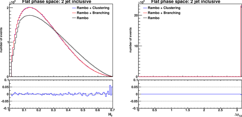
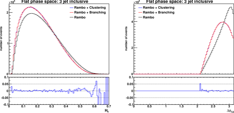
Figure 1: The $H_{T}$ and $\Delta\phi_{12}$ pure phase-space comparisons between clustered $(n+1)$-particle Rambo events (blue lines) and forward-branched $n$-particle Rambo events (red lines) for $n=2$-jet (upper graphs) and $n=3$-jet (lower graphs) configurations. The lower panels show the ratio between the clustered and branched predictions minus one. The black lines represent the results of the corresponding $n$-particle Rambo generations. To focus on the phase-space validation, the matrix-element and PDF weights have not been included in these calculations.

We want to verify the FBPS generator on itself, before we use the generator to calculate the $K$-factor for an $n$-jet phase-space point. For this purpose we do not add in the contributions stemming from the matrix elements and PDFs. This is an important validation to ensure the correct treatment of the weight generation during the build-up of the bremsstrahlung phase space. We use the flat phase-space generator Rambo [67] for the numerical validation of the FBPS generator. The phase space generated by Rambo, $d\,{\mathcal{R}}_{n}$, is connected to the customary flat phase space $d\,\Phi$ through:

$$d\,\Phi\big{(}x_{a}P_{a},x_{b}P_{b}\mapsto J_{1},\ldots,J_{n}\big{)}\;=\;$$ (28)

$$\left(\frac{\pi}{2}\right)^{(n-1)}\left(\frac{(x_{a}x_{b}\,S)^{(n-2)}}{(n-1)!\,(n-2)!}\right)\ d\,{\mathcal{R}}_{n}\big{(}x_{a}P_{a},x_{b}P_{b}\mapsto J_{1},\ldots,J_{n}\big{)}\ .$$

For this test, we do not include parton density functions; instead we choose the parton fractions uniformly between zero and one. We define an $n$-jet event at collider energy of 7 TeV using the following selection criteria for the $n$ jets regarding their transverse momentum, rapidity and geometrical jet–jet separation: $p^{(i)}_{T}>250$ GeV, $|\,\!y_{i}|<2.0$ and $\Delta R_{ij}>0.5$. We present the results of our tests in Figures 1 and 2 where we exemplify the FBPS validation by means of comparisons of distributions for two distinct observables. Here, we define

$$H_{T}\;=\;\sqrt{\frac{\sum\limits_{i}\left|\vec{p}^{\,(i)}_{T}\right|^{2}}{S}}\ ,$$ (29)

as a dimensionless (scaled) variant of an ordinary $H_{T}$ variable where instead of using the scalar sum of the jet $p_{T}$s, the squared quantities have been summed up. With the second observable, we want to look into an angular distribution, namely the azimuthal angle between the two leading jets. This variable is calculated by

$$\Delta\phi_{12}\;=\;\arccos{\left(\frac{\;\;\vec{p}^{\,(1)}_{T}\cdot\vec{p}^{\,(2)}_{T}\;}{\;|\vec{p}^{\,(1)}_{T}|\,|\vec{p}^{\,(2)}_{T}|\;}\right)}\ .$$ (30)

For various $n$-jet final states, the $H_{T}$ and $\Delta\phi_{12}$ distributions resulting from our phase-space tests are displayed in Figures 1 and 2. All plots contain three curves labeled by “Rambo”, “Rambo+Branching” and “Rambo+Clustering” (represented by the black, red and blue lines, respectively); in the corresponding lower panes, we always show the ratio, subtracted by one, between the latter two predictions. In general we observe steeper tails in the $H_{T}$ spectra for an increasing number of jets. The $\Delta\phi_{12}$ distributions show the opposite behavior; their low angle-difference bins become more populated owing to a larger amount of phase space being filled. For the same reason of enhanced phase-space filling, the total energy is shared among more jets, which leads to the suppression of the $H_{T}$ tails.

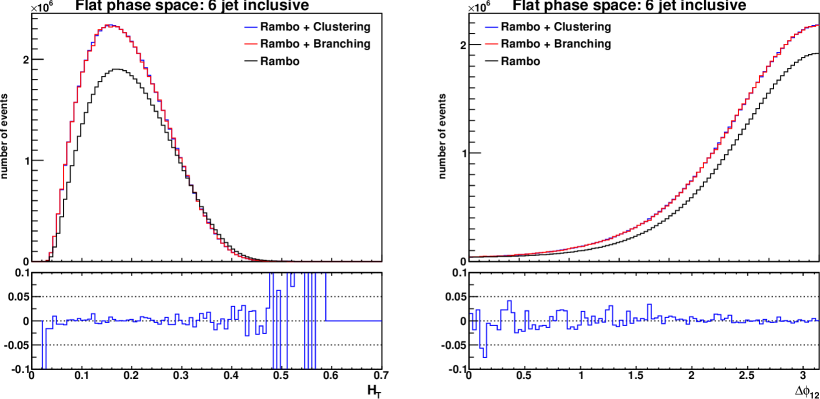
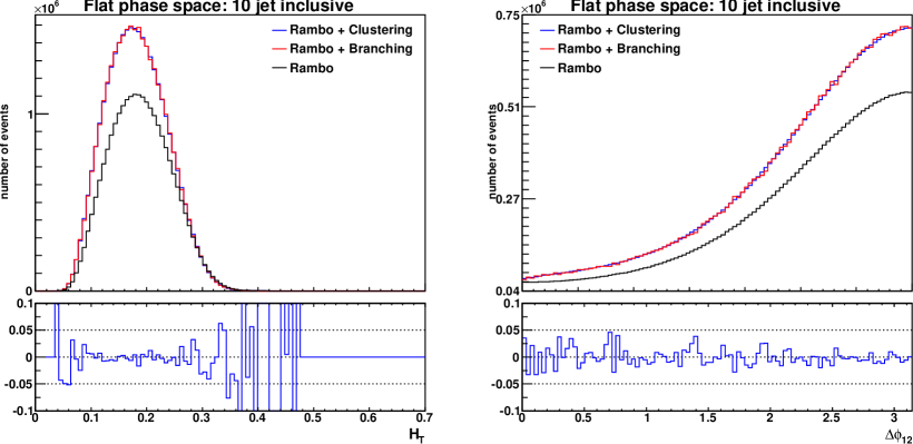
Figure 2: The $H_{T}$ and $\Delta\phi_{12}$ pure phase-space comparisons between clustered $(n+1)$-particle Rambo events (blue lines) and forward-branched $n$-particle Rambo events (red lines) for $n=6$-jet (upper graphs) and $n=10$-jet (lower graphs) configurations. The lower panels show the ratio between the clustered and branched predictions minus one. The black lines represent the results of the corresponding $n$-particle Rambo generations. To focus on the phase-space validation, the matrix-element and PDF weights have not been included in these calculations.

We now explain the three different predictions, which we use for the validation and show in the figures. The “Rambo” curves are obtained from jet momenta generated according to Eq. (28) where we define the “LO” $n$-jet phase space as the $n$-particle uniform phase space. The jet momenta satisfy the acceptance cuts given above. To produce the “NLO” $n$-jet phase space, we generate $n+1$ particles in flat phase space with the help of Rambo and apply our jet algorithm to find $n$ jets from which we can calculate the jet observables. Again, these jets have to fulfill the acceptance criteria. This procedure gives us the “Rambo+Clustering” predictions in Figures 1 and 2. The differences seen between “Rambo” and “Rambo+Clustering” visualize the pure phase-space effect when generating the “NLO” corrections.

We can now validate the FBPS generator: we construct “LO” $n$-jet configurations using the flat phase-space generator as we did for the “Rambo” predictions. For each configuration, we subsequently generate bremsstrahlung events using the FBPS. As the generated events always reconstruct back to the originating $n$-jet event, we only have to average over the generated event weights. This determines the “Rambo+Branching” curves, which have to coincide – apart from statistical fluctuations – with the respective curves of the “Rambo+Clustering” procedure. The ratio plots in Figures 1 and 2 illustrate how well this is achieved by directly comparing the flat phase-space “NLO” predictions and the FBPS generated “NLO” predictions. We see excellent agreement between the two results and thereby validate the FBPS generator. It is interesting to note that at “NLO” the $\Delta\phi_{12}$ distribution for two jets does not show the usual feature of de-correlating. Because the jet algorithm is infra-red safe for all jet observables, the two jets are always exactly back-to-back (in the azimuthal angle) for both “LO” and “NLO”, i.e. this dijet observable is not affected by the initial-state radiation.

4 The Gluonic Jet Generator

As a proof-of-principle we describe in this section a generator, which calculates the NLO $K$-factor per jet phase-space point for the pure gluonic part of $n$-jet production at hadron colliders in the leading-color approximation.

The determination of the $K$-factor for a given $n$-jet event requires the evaluation of a single virtual event and a three-dimensional Monte Carlo integration over the bremsstrahlung phase-space sectors defined by the jet resolution scale. This is discussed in Section 4.1. Finally, in Section 4.2 our results are presented: we verify the cancellation of the slicing parameter in the $K$-factor and the evaluation of the full leading-color NLO corrections up to $15$-jet configurations.

4.1 Evaluation of the $K$-factor

In terms of ordered amplitudes $m$, the fully differential gluonic leading-order, leading-color contribution to the $n$-jet cross section is given as

$$\frac{d^{(n)}\sigma_{\textrm{\tiny LO}}}{d\,J_{1}\cdots d\,J_{n}} = \frac{(2\pi)^{4-3n}}{2\,x_{a}x_{b}\,S}\ F_{g}(x_{a})\,F_{g}(x_{b})\ N_{\mathrm{C}}^{n}\left(N^{2}_{\mathrm{C}}-1\right)$$ (31)

$$\times \left[\,\sum_{\sigma\,\in\,S_{n+1}}\left|\overline{m}^{(0)}\big{(}x_{a}P_{a},J_{\sigma_{1}},J_{\sigma_{2}},\ldots,J_{\sigma_{n+1}}\big{)}\right|^{2}\;+\;{\mathcal{O}}\left(\frac{1}{N_{\mathrm{C}}^{2}}\right)\,\right]\ ,$$

where the color, $N_{\mathrm{C}}$, dependence has been made explicit. The sum is over all $(n+1)!$ different permutations of the ordered amplitudes and the $|\overline{m}^{(0)}|^{2}$ are the corresponding helicity averaged/summed squared matrix elements. Note that the $\sigma_{i}$ take values from $b,1,\ldots,n$ where $J_{b}=x_{b}P_{b}$. We can now define the fully differential NLO cross section through ordered $k$-factors,

$$\frac{d^{(n)}\sigma_{\textrm{\tiny NLO}}}{d\,J_{1}\cdots d\,J_{n}}\;\,=\;\,\frac{(2\pi)^{4-3n}}{2\,x_{a}x_{b}\,S}\ F_{g}(x_{a})\,F_{g}(x_{b})\ N_{\mathrm{C}}^{n}\left(N^{2}_{\mathrm{C}}-1\right)\;\,\times$$ (32)

$$\left[\,\sum_{\sigma\,\in\,S_{n+1}}\overline{k}_{\textrm{\tiny NLO}}\big{(}J_{a},J_{\sigma_{1}},J_{\sigma_{2}},\ldots,J_{\sigma_{n+1}}\big{)}\left|\overline{m}^{(0)}\big{(}J_{a},J_{\sigma_{1}},J_{\sigma_{2}},\ldots,J_{\sigma_{n+1}}\big{)}\right|^{2}\,+\;{\mathcal{O}}\left(\frac{1}{N_{\mathrm{C}}^{2}}\right)\vphantom{\sum_{\sigma\,\in\,S_{n+1}}}\right]$$

with $J_{a}=x_{a}P_{a}$. Notice that each ordering has been assigned its own $k$-factor.

We further detail the ordered $k$-factor similar to Eq. (13) by dividing the virtual contribution into two parts, which we call $v_{\textrm{\tiny D}}$ and $f$. The former is proportional to the LO term and contains the singularities; the latter describes the finite virtual corrections. We now furthermore specify helicity dependent $k$-factors and write representative for all orderings

$$k_{\textrm{\tiny NLO}}\big{(}J_{a}^{\lambda_{a}},J_{b}^{\lambda_{b}},J_{1}^{\lambda_{1}},\ldots,J_{n}^{\lambda_{n}}\big{)}\;\,=\;\,1\;+\;\left(\frac{\alpha_{S}N_{\mathrm{C}}}{2\pi}\right)\times$$ (33)

$$\left(v_{\textrm{\tiny D}}\big{(}J_{a},J_{b},J_{1},\ldots,J_{n}\big{)}\;+\;r\big{(}J_{a},J_{b},J_{1},\ldots,J_{n}\big{)}\;+\;\hat{f}\big{(}J_{a}^{\lambda_{a}},J_{b}^{\lambda_{b}},J_{1}^{\lambda_{1}},\ldots,J_{n}^{\lambda_{n}}\big{)}\right)\ ,$$

where

$$\hat{f}\big{(}J_{a}^{\lambda_{a}},J_{b}^{\lambda_{b}},J_{1}^{\lambda_{1}},\ldots,J_{n}^{\lambda_{n}}\big{)}\;=\;\frac{f\big{(}J_{a}^{\lambda_{a}},J_{b}^{\lambda_{b}},J_{1}^{\lambda_{1}},\ldots,J_{n}^{\lambda_{n}}\big{)}}{\left|m^{(0)}\big{(}J_{a}^{\lambda_{a}},J_{b}^{\lambda_{b}},J_{1}^{\lambda_{1}},\ldots,J_{n}^{\lambda_{n}}\big{)}\right|^{2}}\ .$$ (34)

Note that the $v_{\textrm{\tiny D}}$ part is independent of the helicity structure and is known in analytical form [72, 73]. The helicity information is carried by the LO amplitude. We use the code of Ref. [5] to calculate the finite, helicity dependent contribution $f$. The unresolved soft/collinear contributions contained in $r$ are obtained using a phase-space slicing method [72, 73]. Similarly to the singular virtual terms, this analytically calculated contribution is helicity independent and proportional to the Born level expression. We add it to the $v_{\textrm{\tiny D}}$ term, which now becomes dependent on the slicing parameter: $v_{\textrm{\tiny D}}\to v_{\textrm{\tiny D}}(s_{\mathrm{min}})$, while the resolved contribution is contained in $r\to r(s_{\mathrm{min}})$. The ordered resolved bremsstrahlung factor $r(s_{\mathrm{min}})$ is defined such that it is independent of the helicity choice. This is done in the same manner as for the unordered bremsstrahlung factor $R=\frac{2\pi\,\widetilde{R}}{\alpha_{S}N_{\mathrm{C}}}$ in Eq. (3.2). We define the bremsstrahlung factor as the ratio of the helicity summed bremsstrahlung contribution divided by the helicity summed LO contribution, schematically written as $|m_{\textrm{brems}}^{\lambda_{1},\ldots,\lambda_{n}}|^{2}\equiv\big{(}\sum_{\kappa}|m_{\textrm{brems}}^{\kappa_{1},\ldots,\kappa_{n+1}}|^{2}/\sum_{\kappa}|m_{\textrm{\tiny LO}}^{\kappa_{1},\ldots,\kappa_{n}}|^{2}\big{)}\times|m_{\textrm{\tiny LO}}^{\lambda_{1},\ldots,\lambda_{n}}|^{2}$. By doing so we have arranged for having all the helicity dependence carried by the jets $J_{1},\ldots,J_{n}$, i.e. the Born level ordered amplitude. This approach of defining the helicity dependence gives us the correct behavior: the soft/collinear limit is found to be proportional to the LO helicity dependent ordered amplitude. Furthermore, if the helicity sum over the jets is carried out, one retrieves the helicity summed bremsstrahlung amplitude.

At this level of the Monte Carlo program development, it is convenient to have an explicit $\log^{2}(s_{\mathrm{min}})$ dependence in the unresolved parton contribution. In the previous section we validated the FBPS generator based on and using flat phase-space generation. However, the soft/collinear limit is hardly probed by distributing the momenta uniformly in phase space. As the $s_{\mathrm{min}}$ dependence of the $v_{\textrm{\tiny D}}$ part has to cancel against that of the FBPS generator, we get an excellent probe on the crucial correctness of the soft/collinear behavior of the FBPS generator.

In the future we can switch to a subtraction method, eliminating the dependence on the slicing parameter. For the class of infra-red safe jet algorithms, this is almost trivial. The observable jet final state is invariant under the bremsstrahlung Monte Carlo integration. This means we only have to add to the $k$-factor, an integral over the unresolved phase space. The integrand is simply given by the difference between the bremsstrahlung matrix element squared and its antenna approximation. The $s_{\mathrm{min}}$ parameter then becomes equivalent to the so-called $\alpha$ parameter introduced in Ref. [85].

4.2 Numerical studies of NLO high multiplicity jet events

         

         

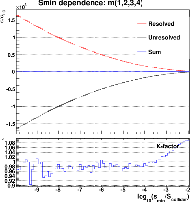
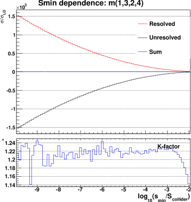
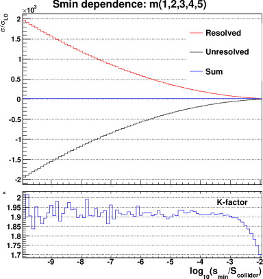
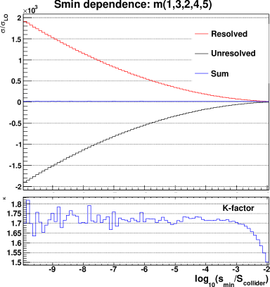
Figure 3: The cancellation of the $s_{\mathrm{min}}$ dependence for the 2-jet and 3-jet configurations given in Appendix B. The upper panels show the resolved contribution in red, the unresolved contribution in black and the helicity independent part of the $k$-factor defined in Eq. (33) in blue. In the lower panel, the dependence on $s_{\mathrm{min}}$ of the helicity independent part of the $k$-factor is shown in finer detail. The different color orderings (indicated in the respective plot titles) use the same events in the Monte Carlo evaluation, leading to correlated statistical fluctuations.

For all numerical studies we use single, exclusive $n$-jet events. As for the numerical validation of the FBPS generator in Section 3.4, all events pass the jet cuts $p^{(i)}_{T}>250$ GeV, $|\,\!y_{i}|<2.0$ and $\Delta R_{ij}>0.5$ at a collider energy of 7 TeV using the CTEQ6M PDF set [86]. The renormalization/factorization scale is set to one half times the average dijet mass. This scale choice is closely connected to shower Monte Carlo approaches where the dijet mass is often used as the starting scale for branchings off the particular dipole antenna.

         

         

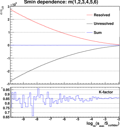
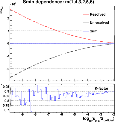
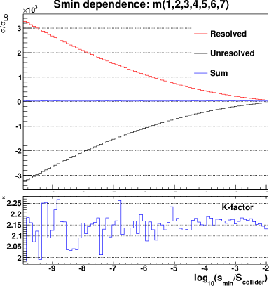
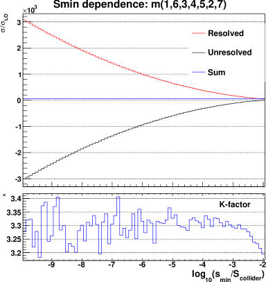
Figure 4: The cancellation of the $s_{\mathrm{min}}$ dependence for the 4-jet and 5-jet configurations given in Appendix B. The upper panels show the resolved contribution in red, the unresolved contribution in black and the helicity independent part of the $k$-factor defined in Eq. (33) in blue. In the lower panel, the dependence on $s_{\mathrm{min}}$ of the helicity independent part of the $k$-factor is shown in finer detail. The different color orderings (indicated in the respective plot titles) use the same events in the Monte Carlo evaluation, leading to correlated statistical fluctuations.

We first have to study the dependence on the slicing parameter $s_{\mathrm{min}}$ for explicit jet configurations. To this end we calculate the resolved, $r(s_{\mathrm{min}})$, and the unresolved, $v_{\textrm{\tiny D}}(s_{\mathrm{min}})$, helicity independent contributions to the $k$-factor. The results are shown in Figures 3, 4 and 5 together with the helicity independent part of the $k$-factor, $1+\left(\frac{\alpha_{S}N_{\mathrm{C}}}{2\pi}\right)\big{[}r(s_{\mathrm{min}})+v_{\textrm{\tiny D}}(s_{\mathrm{min}})\big{]}$, for a single $2$-jet, $3$-jet, $4$-jet, $5$-jet and $8$-jet event and two different orderings per kinematic configuration. The notation in the figures is such that $m^{(0)}(1,2,\ldots,n+2)\equiv m^{(0)}(J_{a},J_{b},J_{1},\ldots,J_{n})$ with $1\leftrightarrow a$, $2\leftrightarrow b$, $3\leftrightarrow 1$ etc. For each antenna, we only have to perform a three-parameter integral, giving us good control over the cancellations. The graphs demonstrate that the cancellation of the $s_{\mathrm{min}}$ parameter dependence is achieved in a satisfactory manner at values of the order of $10^{-4}\times S$ and smaller. Moreover, we were able to maintain good numerical stability down to values of $s_{\mathrm{min}}<10^{-9}\times S$ ($=S_{\mathrm{collider}}$ in the figures), even though we did not use any adaptive Monte Carlo integration such as Vegas [87] to obtain these results.

		$--++\cdots+$		$---+\cdots++$		$-+-+\cdots-+$
jets	$r$-factor	$\left|m^{(0)}\right|^{2}$	$k$-factor	$\left|m^{(0)}\right|^{2}$	$k$-factor	$\left|m^{(0)}\right|^{2}$	$k$-factor
2	172$\pm$ 1	1.72216	1.15$\pm$ 0.05	1.6$\times 10^{-31}$	$---$	0.00552438	1.09$\pm$ 0.05
3	243$\pm$ 2	120.638	1.13$\pm$ 0.08	0.043632	1.18$\pm$ 0.08	5.98249	1.10$\pm$ 0.08
4	392$\pm$ 3	125.234	1.30$\pm$ 0.13	0.282847	1.17$\pm$ 0.13	0.0498892	1.18$\pm$ 0.13
5	366$\pm$ 4	5941.55	0.94$\pm$ 0.17	849.054	0.87$\pm$ 0.17	31.5083	0.80$\pm$ 0.17
6	529$\pm$ 5	1202.54	1.15$\pm$ 0.24	69.0066	1.06$\pm$ 0.24	0.469815	0.82$\pm$ 0.24
8	650$\pm$ 7	26732.0	1.41$\pm$ 0.34	1364.49	1.32$\pm$ 0.34	1.41604	1.15$\pm$ 0.34
10	844$\pm$ 11	6575.23	1.49$\pm$ 0.49	579.066	1.26$\pm$ 0.49	6.09232$\times 10^{-6}$	0.97$\pm$ 0.49
15	1264$\pm$20	4690.02	1.39$\pm$ 0.95	671.554	1.28$\pm$ 0.95	4.37178$\times 10^{-7}$	1.24$\pm$ 0.95

Table 1: The LO ordered amplitude squared $|m^{(0)}(J_{a},J_{b},J_{1},\ldots,J_{n})|^{2}$ and its corresponding $r(s_{\mathrm{min}})$ and ordered $k$-factor as defined in Eq. (33) for an exclusive $n$-jet event. The explicit jet momenta for the different jet multiplicities are given in Appendix B. The slicing scale $s_{\mathrm{min}}$ is set to $10^{-4}\times S$ and the Monte Carlo integration over the bremsstrahlung phase space has been done with 100,000 generated events.

         

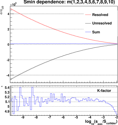
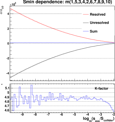
Figure 5: The cancellation of the $s_{\mathrm{min}}$ dependence for the 8-jet configurations given in Appendix B. The upper panels show the resolved contribution in red, the unresolved contribution in black and the helicity independent part of the $k$-factor defined in Eq. (33) in blue. In the lower panel, the dependence on $s_{\mathrm{min}}$ of the helicity independent part of the $k$-factor is shown in finer detail. The different color orderings (indicated in the respective plot titles) use the same events in the Monte Carlo evaluation, leading to correlated statistical fluctuations.

We can now proceed to make some predictions for the $n$-jet configurations listed in Appendix B. In Table 1 we show the results for several helicity configurations of the calculations of the $k$-factors defined in Eq. (33) multiplying the ordered amplitudes squared. As can be seen from the table, the scale choice described above leads to relatively small $k$-factors, i.e. the normalization of the LO prediction is fairly close to the NLO rate. In other words, the correction of the LO weight due to radiative corrections is of the order of one. In addition to the $k$-factors, our table also displays the numerical results $r(s_{\mathrm{min}})$ of the bremsstrahlung phase-space integration using the FBPS generator. As expected, for a fixed number of bremsstrahlung events, the uncertainty on the integration results scales with the square root of the number of dipoles, i.e. it grows linearly in the number of final-state jets (except for the two highest jet multiplicities, where with the chosen number of events we did not achieve a sufficient accuracy for determining a reliable uncertainty estimate). The number of final–final and initial–final dipoles is $n(n-1)$ and $2n$, respectively. To obtain an integration uncertainty independent of the $n$-jet multiplicity, we would have to scale the number of bremsstrahlung events evaluated in the Monte Carlo integration as $n(n-1)+2n=n(n+1)$.

From Table 1 one also reads off that the relative errors on the $k$-factors become sizeable for a large number of jets. This is when the values of the $r$-factors turn big and one finds large cancellations between the single terms in Eq. (33). Owing to the use of a slicing method and its explicit dependence on $\log(s_{\mathrm{min}})$, we are not able to avoid this behavior easily without switching to an approach based on subtractions. Because of these large cancellations, the absolute values of $\Delta r$ multiplied by $\left(\frac{\alpha_{S}N_{\mathrm{C}}}{2\pi}\right)\sim 1/20$ are hence pivotal in determining the uncertainty on the $k$-factors.

5 Conclusions

In this paper we derived a new type of NLO phase-space generator. This forward-branching phase-space generator has the property of inverting the clustering occurring in the jet algorithm. Because of this, the bremsstrahlung phase space of a fully exclusive jet final state is generated. The bremsstrahlung events constructed in this way do not change the value of a jet observable; they are all added to the single virtual contribution. This gives a perfect cancellation of the divergent pieces – the soft/collinear real and virtual contributions – as dictated by the KLN theorem for any jet observable.

However, the current jet algorithms used by the experiments employ a $2\to 1$ clustering scheme. Furthermore, a beam jet is not defined leading to transverse momentum imbalance in jet events. As a result the LO and NLO jet phase spaces are different and only match at the soft/collinear boundary. This makes the jet observables infra-red finite, but not necessarily infra-red safe. The KLN theorem becomes applicable only after some phase-space averaging. As a consequence, the fully exclusive multi-jet event is not defined at NLO.

Any infra-red finite jet algorithm using a $3\rightarrow 2$ clustering scheme, which includes beam jets, suffices to define the fully exclusive multi-jet differential cross section. For the purposes of this paper, we worked out a theoretically simple jet algorithm such that fully exclusive jet final states can be defined at NLO. Nevertheless, the difference between an observable determined by this more theoretical jet algorithm and one currently used by the experiments amounts to a finite correction. This correction is readily calculated for a particular observable by an extra bremsstrahlung phase-space integration, extending the applicability of the forward-branching phase-space generator beyond jet algorithms using $3\rightarrow 2$ clustering schemes.

Since the forward-branching bremsstrahlung phase-space generator does not alter the jet configuration, a $K$-factor can be defined for a given multi-jet phase-space point. The $K$-factor can be determined from the leading-order probability associated with the particular jet phase-space point. In this sense, the probabilistic interpretation of the NLO prediction is restored by quantifying it as a positive-weight adjustment. We validated our method in two steps: first, we verified the construction of the bremsstrahlung phase space; second, we calculated the radiative corrections for individual events with up to $15$ jets. As our test scenario, we chose $2\to n$ gluon production in the leading-color approximation.

Appendix A The Enumeration of Branchings

We can choose the branching pair of jets in Eq. (3.2) by Monte Carlo means. However, it is useful to control the ratio of initial–final and final–final branchings for optimization purposes. This ratio is given by the number of ways the $n+3$ partons can be clustered to $n$ jets plus $2$ incoming partons. If no flavor constraints are taken into account, the derivation of the ratio for the jet algorithm used in this paper goes as follows:

• Given an initial-state parton, there are $n\,(n+1)$ possible clusterings since it is the final-state parton pair that effectively gets combined. This number is based on treating all final-state partons as distinguishable particles. The recoil is taken by one of the two partons in the initial state, giving the number of initial–final state clusterings $N_{\textrm{\tiny IF}}=2\,n\,(n+1)$.

• The number of final–final state clusterings is given by $n\,(n+1)$. For each of these clusterings, we have $n-1$ remaining possible recoil partons. For the number of final-state clusterings, we hence obtain $N_{\textrm{\tiny FF}}=(n-1)\,n\,(n+1)$.

• Accordingly, the total number of possible clusterings is $N_{\mathrm{tot}}=N_{\textrm{\tiny IF}}+N_{\textrm{\tiny FF}}=n\,(n+1)^{2}$.

• Following these observations, the fraction of final–final state branchings to be generated is then given by $N_{\textrm{\tiny FF}}/N_{\mathrm{tot}}=(n-1)/(n+1)$. Similarly, the fraction of initial–final state branchings thus is $N_{\textrm{\tiny IF}}/N_{\mathrm{tot}}=2/(n+1)$. As we see for a very large number of jets, the fraction of pure final-state branchings tends towards one as expected.

Note that in Eq. (3.2) we see that each dipole term is “averaged” by exactly the number of final–final state dipoles, $N_{\textrm{\tiny FF}}$, or the number of initial–final state dipoles per beam, $\frac{1}{2}N_{\textrm{\tiny IF}}$.

Appendix B The Explicit Jet Events

The jet configurations used to calculate the results in Table 1 are given in this appendix, together with some kinematic properties of the particular $n$-jet event. These properties are calculated from the final-state jets.

• For $n=2$, we have:

  $$\alpha_{S}\left(\frac{1}{2}\langle m_{jj}\rangle\right) = 0.0854525\ ,\quad\langle m_{jj}\rangle\;=\;2320.1\ \mathrm{GeV}\ ,$$

  $$\min\left(m_{jj}\right) = 2320.1\ \mathrm{GeV}\ ,\quad\max\left(m_{jj}\right)\;=\;2320.1\ \mathrm{GeV}$$ (35)

  and the momenta (in GeV) are given by

  $$x_{a}\,P_{a} = (651.429,651.429,0,0)\ ,$$

  $$x_{b}\,P_{b} = (2065.78,-2065.78,0,0)\ ,$$

  $$J_{1} = (988.026,4.76957,150.427,976.496)\ ,$$

  $$J_{2} = (1729.19,-1419.12,-150.427,-976.496)\ .$$ (36)

• For $n=3$, we have:

  $$\alpha_{S}\left(\frac{1}{2}\langle m_{jj}\rangle\right) = 0.08936\ ,\quad\langle m_{jj}\rangle\;=\;1546.75\ \mathrm{GeV}\ ,$$

  $$\min\left(m_{jj}\right) = 837.178\ \mathrm{GeV}\ ,\quad\max\left(m_{jj}\right)\;=\;2342.36\ \mathrm{GeV}$$ (37)

  and the momenta (in GeV) are given by

  $$x_{a}\,P_{a} = (1002.78,1002.78,0,0)\ ,$$

  $$x_{b}\,P_{b} = (1789.36,-1789.36,0,0)\ ,$$

  $$J_{1} = (1203.62,-339.322,1151.26,-90.3834)\ ,$$

  $$J_{2} = (1243.44,-297.018,-1187.58,-218.141)\ ,$$

  $$J_{3} = (345.076,-150.236,36.3206,308.525)\ .$$ (38)

• For $n=4$, we have:

  $$\alpha_{S}\left(\frac{1}{2}\langle m_{jj}\rangle\right) = 0.0873363\ ,\quad\langle m_{jj}\rangle\;=\;1899.39\ \mathrm{GeV}\ ,$$

  $$\min\left(m_{jj}\right) = 906.006\ \mathrm{GeV}\ ,\quad\max\left(m_{jj}\right)\;=\;2636.08\ \mathrm{GeV}$$ (39)

  and the momenta (in GeV) are given by

  $$x_{a}\,P_{a} = (2293.54,2293.54,0,0)\ ,$$

  $$x_{b}\,P_{b} = (2359.46,-2359.46,0,0)\ ,$$

  $$J_{1} = (1725.71,877.743,982.549,1114.55)\ ,$$

  $$J_{2} = (954.182,356.832,-669.803,-578.359)\ ,$$

  $$J_{3} = (1037.51,-521.634,-809.127,-386.844)\ ,$$

  $$J_{4} = (935.596,-778.871,496.381,-149.35)\ .$$ (40)

• For $n=5$, we have:

  $$\alpha_{S}\left(\frac{1}{2}\langle m_{jj}\rangle\right) = 0.0921983\ ,\quad\langle m_{jj}\rangle\;=\;1074.2\ \mathrm{GeV}\ ,$$

  $$\min\left(m_{jj}\right) = 365.996\ \mathrm{GeV}\ ,\quad\max\left(m_{jj}\right)\;=\;1794.95\ \mathrm{GeV}$$ (41)

  and the momenta (in GeV) are given by

  $$x_{a}\,P_{a} = (883.985,883.985,0,0)\ ,$$

  $$x_{b}\,P_{b} = (3263.37,-3263.37,0,0)\ ,$$

  $$J_{1} = (684.733,-446.345,-519.146,11.084)\ ,$$

  $$J_{2} = (780.483,-90.2618,684.399,-364.149)\ ,$$

  $$J_{3} = (1081.8,-949.154,502.292,130.739)\ ,$$

  $$J_{4} = (458.187,-330.582,216.105,-232.271)\ ,$$

  $$J_{5} = (1142.15,-563.042,-883.651,454.598)\ .$$ (42)

• For $n=6$, we have:

  $$\alpha_{S}\left(\frac{1}{2}\langle m_{jj}\rangle\right) = 0.0898744\ ,\quad\langle m_{jj}\rangle\;=\;1470.28\ \mathrm{GeV}\ ,$$

  $$\min\left(m_{jj}\right) = 372.579\ \mathrm{GeV}\ ,\quad\max\left(m_{jj}\right)\;=\;2307.33\ \mathrm{GeV}$$ (43)

  and the momenta (in GeV) are given by

  $$x_{a}\,P_{a} = (2711.42,2711.42,0,0)\ ,$$

  $$x_{b}\,P_{b} = (2989.73,-2989.73,0,0)\ ,$$

  $$J_{1} = (1305.48,-936.767,-465.008,781.36)\ ,$$

  $$J_{2} = (416.233,43.8532,163.26,-380.359)\ ,$$

  $$J_{3} = (1255.05,418.867,211.911,1163.96)\ ,$$

  $$J_{4} = (809.408,-755.773,-267.267,-111.885)\ ,$$

  $$J_{5} = (1029.43,606.551,515.234,-652.956)\ ,$$

  $$J_{6} = (885.548,344.959,-158.13,-800.121)\ .$$ (44)

• For $n=8$, we have:

  $$\alpha_{S}\left(\frac{1}{2}\langle m_{jj}\rangle\right) = 0.0956911\ ,\quad\langle m_{jj}\rangle\;=\;861.375\ \mathrm{GeV}\ ,$$

  $$\min\left(m_{jj}\right) = 239.955\ \mathrm{GeV}\ ,\quad\max\left(m_{jj}\right)\;=\;1483.52\ \mathrm{GeV}$$ (45)

  and the momenta (in GeV) are given by

  $$x_{a}\,P_{a} = (1566.71,1566.71,0,0)\ ,$$

  $$x_{b}\,P_{b} = (3315.09,-3315.09,0,0)\ ,$$

  $$J_{1} = (771.638,72.2583,756.755,132.381)\ ,$$

  $$J_{2} = (799.106,-447.319,-526.283,-401.875)\ ,$$

  $$J_{3} = (362.664,-225.218,127.162,-254.228)\ ,$$

  $$J_{4} = (455.86,294.142,-344.111,-53.627)\ ,$$

  $$J_{5} = (336.571,-176.658,48.6816,282.315)\ ,$$

  $$J_{6} = (897.978,-705.684,548.115,89.1335)\ ,$$

  $$J_{7} = (897.601,-802.832,-399.01,44.0329)\ ,$$

  $$J_{8} = (360.374,242.933,-211.31,161.867)\ .$$ (46)

• For $n=10$, we have:

  $$\alpha_{S}\left(\frac{1}{2}\langle m_{jj}\rangle\right) = 0.0950109\ ,\quad\langle m_{jj}\rangle\;=\;913.794\ \mathrm{GeV}\ ,$$

  $$\min\left(m_{jj}\right) = 237.586\ \mathrm{GeV}\ ,\quad\max\left(m_{jj}\right)\;=\;1830.56\ \mathrm{GeV}$$ (47)

  and the momenta (in GeV) are given by

  $$x_{a}\,P_{a} = (2827.46,2827.46,0,0)\ ,$$

  $$x_{b}\,P_{b} = (3322.41,-3322.41,0,0)\ ,$$

  $$J_{1} = (547.589,302.187,339.049,305.912)\ ,$$

  $$J_{2} = (956.324,-806.585,389.162,335.454)\ ,$$

  $$J_{3} = (350.22,-95.7603,228.577,247.461)\ ,$$

  $$J_{4} = (259.829,-26.1444,-35.2505,-256.096)\ ,$$

  $$J_{5} = (314.102,-35.8975,4.96171,312.004)\ ,$$

  $$J_{6} = (986.504,-606.912,589.914,-506.804)\ ,$$

  $$J_{7} = (889.429,-326.063,-798.032,-218.89)\ ,$$

  $$J_{8} = (891.285,649.951,-560.226,-241.04)\ ,$$

  $$J_{9} = (518.799,168.343,-476.506,117.284)\ ,$$

  $$J_{10} = (435.784,281.925,318.35,-95.2848)\ .$$ (48)

• For $n=15$, we have:

  $$\alpha_{S}\left(\frac{1}{2}\langle m_{jj}\rangle\right) = 0.0993949\ ,\quad\langle m_{jj}\rangle\;=\;633.545\ \mathrm{GeV}\ ,$$

  $$\min\left(m_{jj}\right) = 147.1\ \mathrm{GeV}\ ,\quad\max\left(m_{jj}\right)\;=\;1497.81\ \mathrm{GeV}$$ (49)

  and the momenta (in GeV) are given by

  $$x_{a}\,P_{a} = (3403.1,3403.1,0,0)\ ,$$

  $$x_{b}\,P_{b} = (3096.06,-3096.06,0,0)\ ,$$

  $$J_{1} = (349.237,141.394,-212.337,-238.51)\ ,$$

  $$J_{2} = (272.807,-73.295,214.113,-152.339)\ ,$$

  $$J_{3} = (465.556,289.402,279.374,234.392)\ ,$$

  $$J_{4} = (269.21,54.8123,-263.571,-0.174956)\ ,$$

  $$J_{5} = (451.568,254.001,87.8387,-362.88)\ ,$$

  $$J_{6} = (437.866,292.297,303.293,-119.594)\ ,$$

  $$J_{7} = (368.167,-241.648,223.073,165.504)\ ,$$

  $$J_{8} = (355.366,-41.1757,-217.718,-277.828)\ ,$$

  $$J_{9} = (328.823,-87.4318,-296.434,-112.281)\ ,$$

  $$J_{10} = (458.585,-188.764,-88.852,408.379)\ ,$$

  $$J_{11} = (332.789,159.417,-133.945,259.603)\ ,$$

  $$J_{12} = (572.199,-470.06,-321.957,-52.8996)\ ,$$

  $$J_{13} = (746.136,-332.113,245.182,-621.534)\ ,$$

  $$J_{14} = (830.982,518.077,212.244,614.069)\ ,$$

  $$J_{15} = (259.874,32.133,-30.3028,256.093)\ .$$ (50)

References

- [1] W. T. Giele and G. Zanderighi, On the Numerical Evaluation of One-Loop Amplitudes: The Gluonic Case, JHEP 06 (2008) 038, [arXiv:0805.2152].
- [2] R. K. Ellis, W. T. Giele, Z. Kunszt, K. Melnikov, and G. Zanderighi, One-loop amplitudes for +3 jet production in hadron collisions, JHEP 01 (2009) 012, [arXiv:0810.2762].
- [3] A. Lazopoulos, Multi-gluon one-loop amplitudes numerically, arXiv:0812.2998.
- [4] R. K. Ellis, K. Melnikov, and G. Zanderighi, Generalized unitarity at work: first NLO QCD results for hadronic +3 jet production, JHEP 04 (2009) 077, [arXiv:0901.4101].
- [5] J. Winter and W. T. Giele, Calculating gluon one-loop amplitudes numerically, arXiv:0902.0094.
- [6] C. F. Berger et. al., Precise Predictions for + 3 Jet Production at Hadron Colliders, Phys. Rev. Lett. 102 (2009) 222001, [arXiv:0902.2760].
- [7] K. Melnikov and M. Schulze, NLO QCD corrections to top quark pair production and decay at hadron colliders, JHEP 08 (2009) 049, [arXiv:0907.3090].
- [8] G. Bevilacqua, M. Czakon, C. G. Papadopoulos, R. Pittau, and M. Worek, Assault on the NLO Wishlist: , JHEP 09 (2009) 109, [arXiv:0907.4723].
- [9] W. Giele, Z. Kunszt, and J. Winter, Efficient Color-Dressed Calculation of Virtual Corrections, Nucl.Phys. B840 (2010) 214–270, [arXiv:0911.1962].
- [10] G. Bevilacqua, M. Czakon, C. Papadopoulos, and M. Worek, Dominant QCD Backgrounds in Higgs Boson Analyses at the LHC: A Study of + 2 jets at Next-To-Leading Order, Phys.Rev.Lett. 104 (2010) 162002, [arXiv:1002.4009].
- [11] C. Berger, Z. Bern, L. J. Dixon, F. Cordero, D. Forde, et. al., Next-to-Leading Order QCD Predictions for Z, + 3-Jet Distributions at the Tevatron, Phys.Rev. D82 (2010) 074002, [arXiv:1004.1659].
- [12] K. Melnikov and M. Schulze, NLO QCD corrections to top quark pair production in association with one hard jet at hadron colliders, Nucl. Phys. B840 (2010) 129–159, [arXiv:1004.3284].
- [13] T. Melia, K. Melnikov, R. Rontsch, and G. Zanderighi, Next-to-leading order QCD predictions for jj production at the LHC, JHEP 12 (2010) 053, [arXiv:1007.5313].
- [14] R. Frederix, S. Frixione, K. Melnikov, and G. Zanderighi, NLO QCD corrections to five-jet production at LEP and the extraction of , JHEP 11 (2010) 050, [arXiv:1008.5313].
- [15] C. Berger, Z. Bern, L. J. Dixon, F. Cordero, D. Forde, et. al., Precise Predictions for + 4 Jet Production at the Large Hadron Collider, Phys.Rev.Lett. 106 (2011) 092001, [arXiv:1009.2338].
- [16] S. Badger, B. Biedermann, and P. Uwer, NGluon: A Package to Calculate One-loop Multi-gluon Amplitudes, Comput.Phys.Commun. 182 (2011) 1674–1692, [arXiv:1011.2900].
- [17] Z. Bern, G. Diana, L. Dixon, F. Cordero, D. Forde, et. al., Left-Handed W Bosons at the LHC, arXiv:1103.5445.
- [18] T. Melia, K. Melnikov, R. Rontsch, and G. Zanderighi, NLO QCD corrections for pair production in association with two jets at hadron colliders, arXiv:1104.2327.
- [19] Z. Bern, G. Diana, L. Dixon, F. Cordero, S. Höche, et. al., Driving Missing Data at Next-to-Leading Order, arXiv:1106.1423.
- [20] R. K. Ellis, W. T. Giele, and Z. Kunszt, A Numerical Unitarity Formalism for Evaluating One-Loop Amplitudes, JHEP 03 (2008) 003, [arXiv:0708.2398].
- [21] W. T. Giele, Z. Kunszt, and K. Melnikov, Full one-loop amplitudes from tree amplitudes, JHEP 04 (2008) 049, [arXiv:0801.2237].
- [22] C. F. Berger et. al., An Automated Implementation of On-Shell Methods for One- Loop Amplitudes, Phys. Rev. D78 (2008) 036003, [arXiv:0803.4180].
- [23] R. K. Ellis, W. T. Giele, Z. Kunszt, and K. Melnikov, Masses, fermions and generalized -dimensional unitarity, Nucl. Phys. B822 (2009) 270–282, [arXiv:0806.3467].
- [24] A. van Hameren, C. G. Papadopoulos, and R. Pittau, Automated one-loop calculations: a proof of concept, JHEP 09 (2009) 106, [arXiv:0903.4665].
- [25] P. Mastrolia, G. Ossola, T. Reiter, and F. Tramontano, Scattering AMplitudes from Unitarity-based Reduction Algorithm at the Integrand-level, JHEP 1008 (2010) 080, [arXiv:1006.0710].
- [26] V. Hirschi, R. Frederix, S. Frixione, M. V. Garzelli, F. Maltoni, et. al., Automation of one-loop QCD corrections, JHEP 1105 (2011) 044, [arXiv:1103.0621].
- [27] R. Ellis, Z. Kunszt, K. Melnikov, and G. Zanderighi, One-loop calculations in quantum field theory: from Feynman diagrams to unitarity cuts, arXiv:1105.4319.
- [28] Z. Bern, L. J. Dixon, D. C. Dunbar, and D. A. Kosower, Fusing gauge theory tree amplitudes into loop amplitudes, Nucl. Phys. B435 (1995) 59–101, [hep-ph/9409265].
- [29] R. Britto, E. Buchbinder, F. Cachazo, and B. Feng, One-loop amplitudes of gluons in SQCD, Phys.Rev. D72 (2005) 065012, [hep-ph/0503132].
- [30] G. Ossola, C. G. Papadopoulos, and R. Pittau, Reducing full one-loop amplitudes to scalar integrals at the integrand level, Nucl. Phys. B763 (2007) 147–169, [hep-ph/0609007].
- [31] F. A. Berends and W. T. Giele, Recursive Calculations for Processes with n Gluons, Nucl. Phys. B306 (1988) 759.
- [32] D. A. Kosower, Light Cone Recurrence Relations for QCD Amplitudes, Nucl. Phys. B335 (1990) 23.
- [33] F. Caravaglios and M. Moretti, An algorithm to compute Born scattering amplitudes without Feynman graphs, Phys. Lett. B358 (1995) 332–338, [hep-ph/9507237].
- [34] A. Kanaki and C. G. Papadopoulos, HELAC: A package to compute electroweak helicity amplitudes, Comput. Phys. Commun. 132 (2000) 306–315, [hep-ph/0002082].
- [35] M. Moretti, T. Ohl, and J. Reuter, O’Mega: An optimizing matrix element generator, hep-ph/0102195.
- [36] F. Cachazo, P. Svrcek, and E. Witten, MHV vertices and tree amplitudes in gauge theory, JHEP 09 (2004) 006, [hep-th/0403047].
- [37] K. Risager, A direct proof of the CSW rules, JHEP 12 (2005) 003, [hep-th/0508206].
- [38] R. Britto, F. Cachazo, and B. Feng, New Recursion Relations for Tree Amplitudes of Gluons, Nucl. Phys. B715 (2005) 499–522, [hep-th/0412308].
- [39] R. Britto, F. Cachazo, B. Feng, and E. Witten, Direct Proof Of Tree-Level Recursion Relation In Yang- Mills Theory, Phys. Rev. Lett. 94 (2005) 181602, [hep-th/0501052].
- [40] P. D. Draggiotis, R. H. P. Kleiss, A. Lazopoulos, and C. G. Papadopoulos, Diagrammatic proof of the BCFW recursion relation for gluon amplitudes in QCD, Eur. Phys. J. C46 (2006) 741–750, [hep-ph/0511288].
- [41] D. Vaman and Y.-P. Yao, QCD recursion relations from the largest time equation, JHEP 04 (2006) 030, [hep-th/0512031].
- [42] C. Schwinn and S. Weinzierl, Scalar diagrammatic rules for Born amplitudes in QCD, JHEP 05 (2005) 006, [hep-th/0503015].
- [43] S. Frixione, Z. Kunszt, and A. Signer, Three jet cross-sections to next-to-leading order, Nucl.Phys. B467 (1996) 399–442, [hep-ph/9512328].
- [44] S. Catani and M. H. Seymour, A general algorithm for calculating jet cross sections in NLO QCD, Nucl. Phys. B485 (1997) 291–419, [hep-ph/9605323].
- [45] T. Gleisberg and F. Krauss, Automating dipole subtraction for QCD NLO calculations, Eur. Phys. J. C53 (2008) 501–523, [arXiv:0709.2881].
- [46] R. Frederix, T. Gehrmann, and N. Greiner, Automation of the Dipole Subtraction Method in MadGraph/MadEvent, JHEP 0809 (2008) 122, [arXiv:0808.2128].
- [47] M. Czakon, C. G. Papadopoulos, and M. Worek, Polarizing the Dipoles, JHEP 08 (2009) 085, [arXiv:0905.0883].
- [48] R. Frederix, S. Frixione, F. Maltoni, and T. Stelzer, Automation of next-to-leading order computations in QCD: The FKS subtraction, JHEP 0910 (2009) 003, [arXiv:0908.4272].
- [49] K. Hasegawa, S. Moch, and P. Uwer, AutoDipole - Automated generation of dipole subtraction terms -, Comput. Phys. Commun. 181 (2010) 1802–1817, [arXiv:0911.4371].
- [50] R. Frederix, T. Gehrmann, and N. Greiner, Integrated dipoles with MadDipole in the MadGraph framework, JHEP 06 (2010) 086, [arXiv:1004.2905].
- [51] G. Corcella, I. Knowles, G. Marchesini, S. Moretti, K. Odagiri, et. al., HERWIG 6: An Event generator for hadron emission reactions with interfering gluons (including supersymmetric processes), JHEP 0101 (2001) 010, [hep-ph/0011363].
- [52] M. Bahr, S. Gieseke, M. Gigg, D. Grellscheid, K. Hamilton, et. al., Herwig++ Physics and Manual, Eur.Phys.J. C58 (2008) 639–707, [arXiv:0803.0883].
- [53] T. Sjöstrand, S. Mrenna, and P. Z. Skands, PYTHIA 6.4 Physics and Manual, JHEP 0605 (2006) 026, [hep-ph/0603175].
- [54] T. Sjöstrand, S. Mrenna, and P. Z. Skands, A Brief Introduction to PYTHIA 8.1, Comput.Phys.Commun. 178 (2008) 852–867, [arXiv:0710.3820].
- [55] T. Gleisberg, S. Höche, F. Krauss, A. Schälicke, S. Schumann, et. al., SHERPA 1. alpha: A Proof of concept version, JHEP 0402 (2004) 056, [hep-ph/0311263].
- [56] T. Gleisberg, S. Höche, F. Krauss, M. Schönherr, S. Schumann, et. al., Event generation with SHERPA 1.1, JHEP 0902 (2009) 007, [arXiv:0811.4622].
- [57] A. Buckley, J. Butterworth, S. Gieseke, D. Grellscheid, S. Höche, et. al., General-purpose event generators for LHC physics, Physics Reports (2011) [arXiv:1101.2599].
- [58] C. W. Bauer, F. J. Tackmann, and J. Thaler, GenEvA. II. A Phase space generator from a reweighted parton shower, JHEP 0812 (2008) 011, [arXiv:0801.4028].
- [59] L. Lönnblad, ARIADNE version 4: A Program for simulation of QCD cascades implementing the color dipole model, Comput.Phys.Commun. 71 (1992) 15–31.
- [60] T. Sjöstrand and P. Z. Skands, Transverse-momentum-ordered showers and interleaved multiple interactions, Eur.Phys.J. C39 (2005) 129–154, [hep-ph/0408302].
- [61] W. T. Giele, D. A. Kosower, and P. Z. Skands, A Simple shower and matching algorithm, Phys.Rev. D78 (2008) 014026, [arXiv:0707.3652].
- [62] M. Dinsdale, M. Ternick, and S. Weinzierl, Parton showers from the dipole formalism, Phys.Rev. D76 (2007) 094003, [arXiv:0709.1026].
- [63] S. Schumann and F. Krauss, A Parton shower algorithm based on Catani-Seymour dipole factorisation, JHEP 0803 (2008) 038, [arXiv:0709.1027].
- [64] J. Winter and F. Krauss, Initial-state showering based on colour dipoles connected to incoming parton lines, JHEP 0807 (2008) 040, [arXiv:0712.3913].
- [65] A. J. Larkoski and M. E. Peskin, Spin-Dependent Antenna Splitting Functions, Phys.Rev. D81 (2010) 054010, [arXiv:0908.2450].
- [66] S. Plätzer and S. Gieseke, Coherent Parton Showers with Local Recoils, JHEP 1101 (2011) 024, [arXiv:0909.5593].
- [67] R. Kleiss, W. J. Stirling, and S. D. Ellis, A new Monte Carlo treatment of multiparticle phase space at high-energies, Comput. Phys. Commun. 40 (1986) 359.
- [68] P. D. Draggiotis, A. van Hameren, and R. Kleiss, SARGE: An algorithm for generating QCD antennas, Phys. Lett. B483 (2000) 124–130, [hep-ph/0004047].
- [69] A. van Hameren and C. G. Papadopoulos, A hierarchical phase space generator for QCD antenna structures, Eur. Phys. J. C25 (2002) 563–574, [hep-ph/0204055].
- [70] A. van Hameren, Kaleu: a general-purpose parton-level phase space generator, arXiv:1003.4953.
- [71] M. Cacciari, G. P. Salam, and G. Soyez, The Anti-k(t) jet clustering algorithm, JHEP 0804 (2008) 063, [arXiv:0802.1189].
- [72] W. Giele and E. Glover, Higher order corrections to jet cross-sections in e+ e- annihilation, Phys.Rev. D46 (1992) 1980–2010.
- [73] W. Giele, E. Glover, and D. A. Kosower, Higher order corrections to jet cross-sections in hadron colliders, Nucl.Phys. B403 (1993) 633–670, [hep-ph/9302225].
- [74] S. D. Ellis and D. E. Soper, Triply differential jet cross-sections for hadron collisions at order in QCD, Phys.Rev.Lett. 74 (1995) 5182–5185, [hep-ph/9412342].
- [75] DØ Collaboration, V. M. Abazov et. al., Measurement of dijet azimuthal decorrelations at central rapidities in collisions at TeV, Phys. Rev. Lett. 94 (2005) 221801, [hep-ex/0409040].
- [76] CMS Collaboration, V. Khachatryan et. al., Dijet Azimuthal Decorrelations in Collisions at TeV, Phys.Rev.Lett. 106 (2011) 122003, [arXiv:1101.5029].
- [77] S. Catani, Y. L. Dokshitzer, M. Seymour, and B. Webber, Longitudinally invariant clustering algorithms for hadron hadron collisions, Nucl.Phys. B406 (1993) 187–224.
- [78] S. D. Ellis and D. E. Soper, Successive combination jet algorithm for hadron collisions, Phys.Rev. D48 (1993) 3160–3166, [hep-ph/9305266].
- [79] G. C. Blazey, J. R. Dittmann, S. D. Ellis, V. Elvira, K. Frame, et. al., Run II jet physics, hep-ex/0005012.
- [80] G. P. Salam and G. Soyez, A Practical Seedless Infrared-Safe Cone jet algorithm, JHEP 0705 (2007) 086, [arXiv:0704.0292].
- [81] S. Ellis, J. Huston, K. Hatakeyama, P. Loch, and M. Tonnesmann, Jets in hadron-hadron collisions, Prog.Part.Nucl.Phys. 60 (2008) 484–551, [arXiv:0712.2447].
- [82] L. Lönnblad, ARCLUS: A New jet clustering algorithm inspired by the color dipole model, Z.Phys. C58 (1993) 471–478.
- [83] S. Weinzierl and D. A. Kosower, QCD corrections to four jet production and three jet structure in e+ e- annihilation, Phys.Rev. D60 (1999) 054028, [hep-ph/9901277].
- [84] A. Daleo, T. Gehrmann, and D. Maitre, Antenna subtraction with hadronic initial states, JHEP 04 (2007) 016, [hep-ph/0612257].
- [85] Z. Nagy and Z. Trocsanyi, Next-to-leading order calculation of four jet observables in electron positron annihilation, Phys.Rev. D59 (1999) 014020, [hep-ph/9806317].
- [86] J. Pumplin, D. Stump, J. Huston, H. Lai, P. M. Nadolsky, et. al., New generation of parton distributions with uncertainties from global QCD analysis, JHEP 0207 (2002) 012, [hep-ph/0201195].
- [87] G. P. Lepage, VEGAS: An adaptive multi dimensional integration program, CLNS-80/447.