Optimal high frequency trading with limit and market orders

Abstract

We propose a framework for studying optimal market making policies in a limit order book (LOB). The bid-ask spread of the LOB is modelled by a Markov chain with finite values, multiple of the tick size, and subordinated by the Poisson process of the tick-time clock. We consider a small agent who continuously submits limit buy/sell orders at best bid/ask quotes, and may also set limit orders at best bid (resp. ask) plus (resp. minus) a tick for getting the execution order priority, which is a crucial issue in high frequency trading. By trading with limit orders, the agent faces an execution risk since her orders are executed only when they meet counterpart market orders, which are modelled by Cox processes with intensities depending on the spread and on her limit prices. By holding non-zero positions on the risky asset, the agent is also subject to the inventory risk related to price volatility. Then the agent can also choose to trade with market orders, and therefore get immediate execution, but at a least favorable price because she has to cross the bid-ask spread.

The objective of the market maker is to maximize her expected utility from revenue over a short term horizon by a tradeoff between limit and market orders, while controlling her inventory position. This is formulated as a mixed regime switching regular/impulse control problem that we characterize in terms of quasi-variational system by dynamic programming methods. In the case of a mean-variance criterion with martingale reference price or when the asset price follows a Levy process and with exponential utility criterion, the dynamic programming system can be reduced to a system of simple equations involving only the inventory and spread variables.

Calibration procedures are derived for estimating the transition matrix and intensity parameters for the spread and for Cox processes modelling the execution of limit orders. Several computational tests are performed both on simulated and real data, and illustrate the impact and profit when considering execution priority in limit orders and market orders.

Keywords: Market making, limit order book, inventory risk, point process, stochastic control.

1 Introduction

Most of modern equity exchanges are organized as order driven markets. In such type of markets, the price formation exclusively results from operating a limit order book (LOB), an order crossing mechanism where limit orders are accumulated while waiting to be matched with incoming market orders. Any market participant is able to interact with the LOB by posting either market orders or limit orders.

In this context, market making is a class of strategies that consists in simultaneously posting limit orders to buy and sell during the continuous trading session. By doing so, market makers provide counterpart to any incoming market orders: suppose that an investor $A$ wants to sell one share of a given security at time $t$ and that an investor $B$ wants to buy one share of this security at time $t^{\prime}>t$; if both use market orders, the economic role of the market maker $C$ is to buy the stock as the counterpart of $A$ at time $t$, and carry until date $t^{\prime}$ when she will sell the stock as a counterpart of $B$. The revenue that $C$ obtains for providing this service to final investors is the difference between the two quoted prices at ask (limit order to sell) and bid (limit order to buy), also called the market maker’s spread. This role was traditionally fulfilled by specialist firms, but, due to widespread adoption of electronic trading systems, any market participant is now able to compete for providing liquidity. Moreover, as pointed out by empirical studies (e.g. [11],[9]) and in a recent review [7] from AMF, the French regulator, this renewed competition among liquidity providers causes reduced effective market spreads, and therefore reduced indirect costs for final investors.

Empirical studies (e.g. [11]) also described stylized features of market making strategies. First, market making is typically not directional, in the sense that it does not profit from security price going up or down. Second, market makers keep almost no overnight position, and are unwilling to hold any risky asset at the end of the trading day. Finally, they manage to maintain their inventory, i.e. their position on the risky asset close to zero during the trading day, and often equilibrate their position on several distinct marketplaces, thanks to the use of high-frequency order sending algorithms. Estimations of total annual profit for this class of strategy over all U.S. equity market were around $10$ G$ in 2009 [7].

Popular models of market making strategies were set up using a risk-reward approach. Three distinct sources of risk are usually identified: the inventory risk, the adverse selection risk and the execution risk. The inventory risk [1] is comparable to the market risk, i.e. the risk of holding a long or short position on a risky asset. Moreover, due to the uncertain execution of limit orders, market makers only have partial control on their inventory, and therefore the inventory has a stochastic behavior. The adverse selection risk, popular in economic and econometric litterature, is the risk that market price unfavourably deviates, from the market maker point of view, after their quote was taken. This type of risk appears naturally in models where the market orders flow contains information about the fundamental asset value (e.g. [5]). Finally, the execution risk is the risk that limit orders may not be executed, or be partially executed [10]. Indeed, given an incoming market order, the matching algorithm of LOB determines which limit orders are to be executed according to a price/time priority, and this structure fundamentally impacts the dynamics of executions.

Some of these risks were studied in previous works. The seminal work [1] provided a framework to manage inventory risk in a stylized LOB. The market maker objective is to maximize the expected utility of her terminal profit, in the context of limit orders executions occurring at jump times of Poisson processes. This model shows its efficiency to reduce inventory risk, measured via the variance of terminal wealth, against the symmetric strategy. Several extensions and refinement of this setup can be found in recent litterature: [8] provides simplified solution to the backward optimization, an in-depth discussion of its characteristics and an application to the liquidation problem. In [2], the authors develop a closely related model to solve a liquidation problem, and study continuous limit case. The paper [3] provides a way to include more precise empirical features to this framework by embedding a hidden Markov model for high frequency dynamics of LOB. Some aspects of the execution risk were also studied previously, mainly by considering the trade-off between passive and aggressive execution strategies. In [10], the authors solve the Merton’s portfolio optimization problem in the case where the investor can choose between market orders or limit orders; in [13], the possibility to use market orders in addition to limit orders is also taken into account, in the context of market making in the foreign exchange market. Yet the relation between execution risk and the microstructure of the LOB, and especially the price/time priority is, so far, poorly investigated.

In this paper we develop a new model to address these three sources of risk. The stock mid-price is driven by a general Markov process, and we model the market spread as a discrete Markov chain that jumps according to a stochastic clock. Therefore, the spread takes discrete values in the price grid, multiple of the tick size. We allow the market maker to trade both via limit orders, which execution is uncertain, and via market orders, which execution is immediate but costly. The market maker can post limit orders at best quote or improve this quote by one tick. In this last case, she hopes to capture market order flow of agents who are not yet ready to trade at the best bid/ask quote. Therefore, she faces a trade off between waiting to be executed at the current best price, or improve this best price, and then be more rapidly executed but at a less favorable price. We model the limit orders strategy as continuous controls, due to the fact that these orders can be updated at high frequency at no cost. On the contrary, we model the market orders strategy as impulse controls that can only occur at discrete dates. We also include fixed, per share or proportional fees or rebates coming with each execution. Execution processes, counting the number of executed limit orders, are modelled as Cox processes with intensity depending both on the market maker’s controls and on the market spread. In this context, we optimize the expected utility from profit over a finite time horizon, by choosing optimally between limit and market orders, while controlling the inventory position. We study in detail classical frameworks including mean-variance criterion and exponential utility criterion.

The outline of this paper is as follows. In section 2, we detail the model, and comment its features. We also provide direct calibration methods for all quantities involved in our model. We formulate in Section 3 the optimal market making control problem and derive the associated Hamilton-Jacobi-Bellman quasi variational inequality (HJBQVI) from dynamic programming principle. We show how one can reduce the number of state variables to the inventory and spread for the resolution to this QVI in two standard cases. In the last section 4, we provide some numerical results and empirical performance analysis.

2 A market-making model

2.1 Mid price and spread process

Let us fix a probability space $(\Omega,{\cal F},{\bf P})$ equipped with a filtration $\mathbb{F}$ $=$ $({\cal F}_{t})_{t\geq 0}$ satisfying the usual conditions. It is assumed that all random variables and stochastic processes are defined on the stochastic basis $(\Omega,{\cal F},\mathbb{F},{\bf P})$.

The mid-price of the stock is an exogenous Markov process $P$, with infinitesimal generator ${\cal P}$ and state space $\mathbb{P}$. For example, $P$ is a Lévy process (e.g. an arithmetic Brownian motion), or an exponential of Lévy process (e.g. geometric Brownian motion). In the limit order book (LOB) for this stock, we consider a stochastic bid-ask spread resulting from the behaviour of market participants, taking discrete values, which are finite multiple of the tick size $\delta$ $>$ $0$, and jumping at random times. This is modelled as follows: we first consider the tick time clock associated to a Poisson process $(N_{t})_{t}$ with deterministic intensity $\lambda(t)$, and representing the random times where the buy and sell orders of participants in the market affect the bid-ask spread. We next define a discrete-time stationary Markov chain $(\hat{S}_{n})_{n\in\mathbb{N}}$, valued in the finite state space $\mathbb{S}$ $=$ $\delta\mathbb{I}_{m}$, $\mathbb{I}_{m}$ $:=$ $\{1,\ldots,m\}$, $m$ $\in$ $\mathbb{N}\setminus\{0\}$, with probability transition matrix $(\rho_{ij})_{1\leq i,j\leq M}$, i.e. ${\bf P}[\hat{S}_{n+1}=j\delta|\hat{S}_{n}=i\delta]$ $=$ $\rho_{ij}$, s.t. $\rho_{ii}$ $=$ $0$, independent of $N$, and representing the random spread in tick time. The spread process $(S_{t})_{t}$ in calendar time is then defined as the time-change of $\hat{S}$ by $N$, i.e.

$$S_{t} = \hat{S}_{N_{t}},\;\;\;t\geq 0.$$ (2.1)

Hence, $(S_{t})_{t}$ is a continuous time (inhomogeneous) Markov chain with intensity matrix $R(t)$ $=$ $(r_{ij}(t))_{1\leq i,j\leq m}$, where $r_{ij}(t)$ $=$ $\lambda(t)\rho_{ij}$ for $i\neq j$, and $r_{ii}(t)$ $=$ $-\sum_{j\neq i}r_{ij}(t)$. We assume that $S$ and $P$ are independent. The best-bid and best-ask prices are defined by: $P_{t}^{b}$ $=$ $P_{t}-\frac{S_{t}}{2}$, $P_{t}^{a}$ $=$ $P_{t}+\frac{S_{t}}{2}$.

2.2 Trading strategies in the limit order book

We consider an agent (market maker), who trades the stock using either limit orders or market orders. She may submit limit buy (resp. sell) orders specifying the quantity and the price she is willing to pay (resp. receive) per share, but will be executed only when an incoming sell (resp. buy) market order is matching her limit order. Otherwise, she can post market buy (resp. sell) orders for an immediate execution, but, in this case obtain the opposite best quote, i.e. trades at the best-ask (resp. best bid) price, which is less favorable.

Limit orders strategies. The agent may submit at any time limit buy/sell orders at the current best bid/ask prices (and then has to wait an incoming counterpart market order matching her limit), but also control her own bid and ask price quotes by placing buy (resp. sell) orders at a marginal higher (resp. lower) price than the current best bid (resp. ask), i.e. at $P_{t}^{b_{+}}$ $:=$ $P_{t}^{b}+\delta$ (resp. $P_{t}^{a_{-}}$ $:=$ $P_{t}^{a}-\delta$). Such an alternative choice is used in practice by a market maker to capture market orders flow of undecided traders at the best quotes, hence to get priority in the order execution w.r.t. limit order at current best/ask quotes, and can be taken into account in our modelling with discrete spread of tick size $\delta$.

There is then a tradeoff between a larger performance for a quote at the current best bid (resp. ask) price, and a smaller performance for a quote at a higher bid price, but with faster execution. The submission and cancellation of limit orders are for free, as they provide liquidity to the market, and are thus stimulated. Actually, market makers receive some fixed rebate once their limit orders are executed. The agent is assumed to be small in the sense that she does not influence the bid-ask spread. The limit order strategies are then modelled by a continuous time predictable control process:

$$\alpha_{t}^{make} = (Q_{t}^{b},Q_{t}^{a},L_{t}^{b},L_{t}^{a}),\;\;\;t\geq 0,$$

where $L$ $=$ $(L^{b},L^{a})$ valued in $[0,\bar{\ell}]^{2}$, $\bar{\ell}$ $>$ $0$, represents the size of the limit buy/sell order, and $Q$ $=$ $(Q^{b},Q^{a})$ represent the possible choices of the bid/ask quotes either at best or at marginally improved prices, and valued in ${\cal Q}$ $=$ ${\cal Q}^{b}\times{\cal Q}^{a}$, with ${\cal Q}^{b}$ $=$ $\{Bb,Bb_{+}\}$, ${\cal Q}^{a}$ $=$ $\{Ba,Ba_{-}\}$:

• $Bb$: best-bid quote, and $Bb_{+}$: bid quote at best price plus the tick

• $Ba$: best-ask quote, and $Ba_{-}$: ask quote at best price minus the tick

Notice that when the spread is equal to one tick $\delta$, a bid quote at best price plus the tick is actually equal to the best ask, and will then be considered as a buy market order. Similarly, an ask quote at best price minus the tick becomes a best bid, and is then viewed as a sell market order. In other words, the limit orders $Q_{t}$ $=$ $(Q_{t}^{b},Q_{t}^{a})$ take values in ${\cal Q}(S_{t^{-}})$, where ${\cal Q}(s)$ $=$ ${\cal Q}^{b}\times{\cal Q}^{a}$ when $s$ $>$ $\delta$, ${\cal Q}(s)$ $=$ $\{Bb\}\times\{Ba\}$ when $s$ $=$ $\delta$. We shall denote by ${\cal Q}_{i}^{b}$ $=$ ${\cal Q}^{b}$ for $i$ $>$ $1$, and ${\cal Q}_{i}^{b}$ $=$ $\{Bb\}$ for $i$ $=$ $1$, and similarly for ${\cal Q}_{i}^{a}$ for $i$ $\in$ $\mathbb{I}_{m}$.

We denote at any time $t$ by $\pi^{b}(Q_{t}^{b},P_{t},S_{t})$ and $\pi^{a}(Q_{t}^{a},P_{t},S_{t})$ the bid and ask prices of the market maker, where the functions $\pi^{b}$ (resp. $\pi^{a}$) are defined on ${\cal Q}^{b}\times\mathbb{P}\times\mathbb{S}$ (resp. ${\cal Q}^{a}\times\mathbb{P}\times\mathbb{S}$) by:

$$\pi^{b}(q^{b},p,s) = \left\{\begin{array}[]{cl}p-\frac{s}{2},&\mbox{ for }q^{b}\;=\;Bb\\ p-\frac{s}{2}+\delta&\mbox{ for }q^{b}\;=\;Bb_{+}.\end{array}\right.$$

$$\pi^{a}(q^{a},p,s) = \left\{\begin{array}[]{cl}p+\frac{s}{2},&\mbox{ for }q^{a}\;=\;Ba\\ p+\frac{s}{2}-\delta&\mbox{ for }q^{a}\;=\;Ba_{-}.\end{array}\right.$$

We shall denote by $\pi^{b}_{i}(q^{b},p)$ $=$ $\pi^{b}(q^{b},p,s)$, $\pi^{a}_{i}(q^{a},p)$ $=$ $\pi^{a}(q^{a},p,s)$ for $s$ $=$ $i\delta$, $i$ $\in$ $\mathbb{I}_{m}$.

Remark 2.1

One can take into account proportional rebates received by the market makers, by considering; $\pi^{b}(q^{b},p,s)$ $=$ $(p-\frac{s}{2}+\delta 1_{q^{b}=Bb_{+}})(1-\rho)$, $\pi^{a}(q^{a},p,s)$ $=$ $(p+\frac{s}{2}-\delta 1_{q^{a}=Ba_{-}})(1+\rho)$, for some $\rho$ $\in$ $[0,1)$, or per share rebates with: $\pi^{b}(q^{b},p,s)$ $=$ $p-\frac{s}{2}+\delta 1_{q^{b}=Bb_{+}}-\rho$, $\pi^{a}(q^{a},p,s)$ $=$ $p+\frac{s}{2}-\delta 1_{q^{a}=Ba_{-}}+\rho$, for some $\rho$ $>$ $0$.

The limit orders of the agent are executed when they meet incoming counterpart market orders. Let us then consider the arrivals of market buy and market sell orders, which completely match the limit sell and limit buy orders of the small agent, and modelled by independent Cox processes $N^{a}$ and $N^{b}$. The intensity rate of $N_{t}^{a}$ is given by $\lambda^{a}(Q_{t}^{a},S_{t})$ where $\lambda^{a}$ is a deterministic function of the limit quote sell order, and of the spread, satisfying $\lambda^{a}(Ba,s)$ $<$ $\lambda^{a}(Ba_{-},s)$. This natural condition conveys the price/priority in the order execution in the sense that an agent quoting a limit sell order at ask price $P^{a_{-}}$ will be executed before traders at the higher ask price $P^{a}$, and hence receive more often market buy orders. Typically, one would also expect that $\lambda^{a}$ is nonincreasing w.r.t. the spread, which means that the larger is the spread, the less often the market buy orders arrive. Likewise, we assume that the intensity rate of $N_{t}^{b}$ is given by $\lambda^{b}(Q_{t}^{b},S_{t})$ where $\lambda^{b}$ is a deterministic function of the spread, and $\lambda^{b}(Bb,s)$ $<$ $\lambda^{b}(Bb_{+},s)$. We shall denote by $\lambda^{a}_{i}(q^{a})$ $=$ $\lambda^{a}(q^{a},s)$, $\lambda^{b}_{i}(q^{b})$ $=$ $\lambda^{b}(q^{b},s)$ for $s$ $=$ $i\delta$, $i$ $\in$ $\mathbb{I}_{m}$.

For a limit order strategy $\alpha^{make}$ $=$ $(Q^{b},Q^{a},L^{b},L^{a})$, the cash holdings $X$ and the number of shares $Y$ hold by the agent (also called inventory) follow the dynamics

$$dY_{t} = L_{t}^{b}dN_{t}^{b}-L_{t}^{a}dN_{t}^{a},$$ (2.4)

$$dX_{t} = -\pi^{b}(Q_{t}^{b},P_{t^{-}},S_{t^{-}})L_{t}^{b}dN_{t}^{b}+\pi^{a}(Q_{t}^{a},P_{t^{-}},S_{t^{-}})L_{t}^{a}dN_{t}^{a}.$$ (2.5)

Market order strategies. In addition to market making strategies, the investor may place market orders for an immediate execution reducing her inventory. The submissions of market orders, in contrast to limit orders, take liquidity in the market, and are usually subject to fees. We model market order strategies by an impulse control:

$$\alpha^{take} = (\tau_{n},\zeta_{n})_{n\geq 0},$$

where $(\tau_{n})$ is an increasing sequence of stopping times representing the market order decision times of the investor, and $\zeta_{n}$, $n$ $\geq$ $1$, are ${\cal F}_{\tau_{n}}$-measurable random variables valued in $[-\bar{e},\bar{e}]$, $\bar{e}$ $>$ $0$, and giving the number of stocks purchased at the best-ask price if $\zeta_{n}$ $\geq$ $0$, or selled at the best-bid price if $\zeta_{n}$ $<$ $0$ at these times. Again, we assumed that the agent is small so that her total market order will be executed immediately at the best bid or best ask price. In other words, we only consider a linear market impact, which does not depend on the order size. When posting a market order strategy, the cash holdings and the inventory jump at times $\tau_{n}$ by:

$$Y_{\tau_{n}} = Y_{\tau_{n}^{-}}+\zeta_{n},$$ (2.6)

$$X_{\tau_{n}} = X_{\tau_{n}^{-}}-c(\zeta_{n},P_{\tau_{n}},S_{\tau_{n}})$$ (2.7)

where

$$c(e,p,s) = ep+|e|\frac{s}{2}+\varepsilon$$

represents the (algebraic) cost function indicating the amount to be paid immediately when passing a market order of size $e$, given the mid price $p$, a spread $s$, and a fixed fee $\varepsilon$ $>$ $0$. We shall denote by $c_{i}(e,p)$ $=$ $c(e,p,s)$ for $s$ $=$ $i\delta$, $i$ $\in$ $\mathbb{I}_{m}$.

Remark 2.2

One can also include proportional fees $\rho$ $\in$ $[0,1)$ paid at each market order trading by considering a cost function in the form: $c(e,p,s)$ $=$ $(e+\varepsilon|e|)p+(|e|+\rho e)\frac{s}{2}+\varepsilon$, or fixed fees per share with $c(e,p,s)$ $=$ $ep+|e|(\frac{s}{2}+\rho)+\varepsilon$.

In the sequel, we shall denote by ${\cal A}$ the set of all limit/market order trading strategies $\alpha$ $=$ $(\alpha^{make},\alpha^{take})$.

2.3 Parameters estimation

In most order-driven markets, available data are made up of Level 1 data that contain transaction prices and quantities at best quotes, and of Level 2 data containing the volume updates for the liquidity offered at the $L$ first order book slices ($L$ usually ranges from 5 to 10). In this section, we propose some direct methods for estimating the intensity of the spread Markov chain, and of the execution point processes, based only on the observation of Level 1 data. This has the advantage of low computational cost, since we do not have to deal with the whole volume of Level 2 data. Yet, we mention some recent work on parameters estimation from the whole order book data [4], but involving heavier computations based on integral transforms.

Estimation of spread parameters. Assuming that the spread $S$ is observable, let us define the jump times of the spread process:

$$\theta_{0}\;=\;0,\;\;\;\;\;\theta_{n+1} = \inf\left\{t>\theta_{n}\,:\,S_{t}\neq S_{t-}\right\}\,\,,\,\forall n\geq 1.$$

From these observable quantities, one can reconstruct the processes:

$$N_{t} = \#\left\{\theta_{j}>0\,:\,\theta_{j}\leq t\right\}\,\,,\,t\geq 0,$$

$$\hat{S}_{n} = S_{\theta_{n}}\,\,,\,\;n\geq 0.$$

Then, our goal is to estimate the deterministic intensity of the Poisson process $(N_{t})_{t}$, and the transition matrix of the Markov chain $(\hat{S}_{n})_{n}$ from a path realization with high frequency data of the tick-time clock and spread in tick time over a finite trading time horizon $T$, typically of one day. From the observations of $K$ samples of $\hat{S}_{n}$, $n$ $=$ $1,\ldots,K$, and since the Markov chain $(\hat{S}_{n})$ is stationary, we have a consistent estimator (when $K$ goes to infinity) for the transition probability $\rho_{ij}$ $:=$ ${\bf P}[\hat{S}_{n+1}=j\delta|\hat{S}_{n}=i\delta]$ $=$ ${\bf P}[(\hat{S}_{n+1},\hat{S}_{n})=(j\delta,i\delta)]/{\bf P}[\hat{S}_{n}=i\delta]$ given by:

$$\hat{\rho}_{ij} = \frac{\displaystyle\sum_{n=1}^{K}1_{\{(\hat{S}_{n+1},\hat{S}_{n})=(j\delta,i\delta)\}}}{\displaystyle\sum_{n=1}^{K}1_{\{\hat{S}_{n}=i\delta\}}}$$ (2.8)

For the estimation of the deterministic intensity function $\lambda(t)$ of the (non)homogeneous Poisson process $(N_{t})$, we shall assume in a first approximation a simple natural parametric form. For example, we may assume that $\lambda$ is constant over a trading day, and more realistically for taking into account intra-day seasonality effects, we consider that the tick time clock intensity jumps e.g. every hour of a trading day. We then assume that $\lambda$ is in the form:

$$\lambda(t) = \sum\lambda_{k}1_{\{t_{k}\leq t<t_{k+1}\}}$$

where $(t_{k})_{k}$ is a fixed and known increasing finite sequence of $\mathbb{R}_{+}$ with $t_{0}=0$, and $(\lambda_{k})_{k}$ is an unknown finite sequence of $(0,\infty)$. In other words, the intensity is constant equal to $\lambda_{k}$ over each period $[t_{k},t_{k+1}]$, and by assuming that the interval length $t_{k+1}-t_{k}$ is large w.r.t. the intensity $\lambda_{k}$ (which is the case for high frequency data), we have a consistent estimator of $\lambda_{k}$, for all $k$, and then of $\lambda(t)$ given by:

$$\hat{\lambda}_{k} = \frac{N_{t_{k+1}}-N_{t_{k}}}{t_{k+1}-t_{k}}.$$ (2.9)

We performed these two estimation procedures (2.8) and (2.9) on SOGN.PA stock on April 18, 2011 between 9:30 and 16:30 in Paris local time. We used tick-by-tick level 1 data provided by Quanthouse, and fed via a OneTick Timeseries database.

In table 1, we display the estimated transition matrix: first row and column indicate the spread value $s=i\delta$ and the the cell $ij$ shows $\hat{\rho}_{ij}$. For this stock and at this date, the tick size was $\delta=0.005$ euros, and we restricted our analysis to the first $6$ values of the spread $(m=6)$ due to the small number of data outside this range.

spread	0.005	0.01	0.015	0.02	0.025	0.03
0.005	0	0.410	0.220	0.160	0.142	0.065
0.01	0.201	0	0.435	0.192	0.103	0.067
0.015	0.113	0.221	0	0.4582	0.147	0.059
0.02	0.070	0.085	0.275	0	0.465	0.102
0.025	0.068	0.049	0.073	0.363	0	0.446
0.03	0.077	0.057	0.059	0.112	0.692	0

Table 1: Estimation of the transition matrix $(\rho_{ij})$ for the underlying spread of the stock SOGN.PA on April 18, 2011.

In table 2, we display the estimate for the tick time clock intensity $\lambda(t)$ by assuming that it is piecewise constant and jumps only at 10:30, 11:30, …, 16:30 in Paris local time. In figure 1, we plot the tick time clock intensity by using an affine interpolation, and observed a typical U-pattern. Hence, a further step for the estimation of the intensity could be to specify a parametric form for the intensity function fitting $U$ pattern, e.g. parabolic functions in time, and then use a maximum likelihood method for estimating the parameters.

Time	10:30	11:30	12:30	13:30	14:30	15:30	16:30
Clock Intensity $\lambda(t)$	1.654	0.799	0.516	0.377	0.632	1.305	2.113

Table 2: Estimation of the tick time clock (hourly basis) for the stock SOGN.PA on April 18, 2011. Tick time clock intensity $\lambda(t)$ is expressed in second^-1.

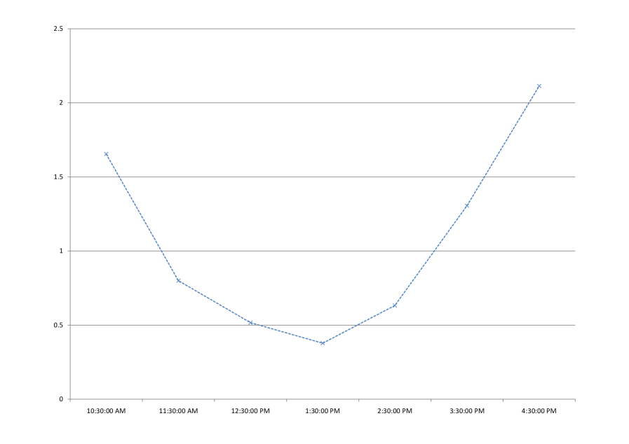
Figure 1: Plot of tick time clock intensity estimate for the stock SOGN.PA on April 18, 2011 expressed in second^-1 (affine interpolation).

Estimation of execution parameters. When performing a limit order strategy $\alpha^{make}$, we suppose that the market maker permanently monitors her execution point processes $N^{a}$ and $N^{b}$, representing respectively the number of arrivals of market buy and sell orders matching the limit orders for quote ask $Q^{a}$ and quote bid $Q^{b}$. We also assume that there is no latency so that the observation of the execution processes is not noisy. Therefore, observable variables include the quintuplet:

$$(N^{a}_{t},N^{b}_{t},Q^{a}_{t},Q^{b}_{t},S_{t})\in\mathbb{R}^{+}\times\mathbb{R}^{+}\times{\cal Q}^{a}\times{\cal Q}^{b}\times\mathbb{S}\,,\,t\in[0,T]$$

Moreover, since $N^{a}$ and $N^{b}$ are assumed to be independent, and both sides of the order book can be estimated using the same procedure, we shall focus on the estimation for the intensity function $\lambda^{b}(q^{b},s)$, $q^{b}$ $\in$ ${\cal Q}^{b}$ $=$ $\{Bb,Bb_{+}\}$, $s$ $\in$ $\mathbb{S}$ $=$ $\delta\mathbb{I}_{m}$, of the Cox process $N^{b}$.

The estimation procedure for $\lambda^{b}(q^{b},s)$ basically matchs the intuition that one must count the number of executions at bid when the system was in the state $(q^{b},s)$ and normalize this quantity by the time spent in the state $(q^{b},s)$. This is justified mathematically as follows. For any $(q^{b},s=i\delta)$ $\in$ ${\cal Q}^{b}\times\mathbb{S}$, let us define the point process

$$N_{t}^{b,q^{b},i} = \int_{0}^{t}1_{\{Q_{u}^{b}=q,S_{u-}=i\delta\}}dN_{u}^{b},\;\;\;t\geq 0,$$

which counts the number of jumps of $N^{b}$ when $(Q^{b},S)$ was in state $(q^{b},s=i\delta)$. Then, for any nonnegative predictable process $(H_{t})$, we have

$${\bf E}\Big{[}\int_{0}^{\infty}H_{t}dN_{t}^{b,q^{b},i}\Big{]} = {\bf E}\Big{[}\int_{0}^{\infty}H_{t}1_{\{Q_{t}^{b}=q^{b},S_{t-}=i\delta\}}dN_{t}^{b}\Big{]}$$ (2.10)

$$= {\bf E}\Big{[}\int_{0}^{\infty}H_{t}1_{\{Q_{t}^{b}=q^{b},S_{t-}=i\delta\}}\lambda^{b}(Q_{t}^{b},S_{t})dt\Big{]}$$

$$= {\bf E}\Big{[}\int_{0}^{\infty}H_{t}1_{\{Q_{t}^{b}=q^{b},S_{t-}=i\delta\}}\lambda_{i}^{b}(q^{b})dt\Big{]},$$

where we used in the second equality the fact that $\lambda^{b}(Q_{t}^{b},S_{t})$ is the intensity of $N^{b}$. The relation (2.10) means that the point process $N^{b,q^{b},i}$ admits for intensity $\lambda_{i}^{b}(q^{b})1_{\{Q_{t}^{b}=q^{b},S_{t-}=i\delta\}}$. By defining

$${\cal T}^{b,q^{b},i}_{t} = \int_{0}^{t}1_{\{Q_{u}^{b}=q,S_{u-}=i\delta\}}du$$

as the time that $(Q^{b},S)$ spent in the state $(q^{b},s=i\delta)$, this means equivalently that the process $M_{t}^{b,q^{b},i}$ $=$ $N^{b,q^{b},i}_{A_{t}^{b,q^{b},i}}$, where $A_{t}^{b,q^{b},i}$ $=$ $\inf\{u\geq 0:{\cal T}_{u}^{b,q^{b},i}\geq t\}$ is the càd-làg inverse of ${\cal T}^{b,q^{b},i}$, is a Poisson process with intensity $\lambda_{i}(q^{b})$. By assuming that ${\cal T}^{b,q^{b},i}_{T}$ is large w.r.t. $\lambda_{i}(q^{b})$, which is the case when $(\hat{S}_{n})$ is irreducible (hence recurrent), and for high-frequency data over $[0,T]$, we have a consistent estimator of $\lambda_{i}^{b}(q^{b})$ given by:

$$\hat{\lambda}_{i}^{b}(q^{b}) = \frac{N_{T}^{b,q^{b},i}}{{\cal T}_{T}^{b,q^{b},i}}.$$ (2.11)

Similarly, we have a consistent estimator for $\lambda_{i}^{a}(q^{a})$ given by:

$$\hat{\lambda}_{i}^{a}(q^{a}) = \frac{N_{T}^{a,q^{a},i}}{{\cal T}_{T}^{a,q^{a},i}},$$ (2.12)

where $N_{T}^{a,q^{a},i}$ counts the number of executions at ask quote $q^{a}$ and for a spread $i\delta$, and ${\cal T}_{T}^{a,q^{a},i}$ is the time that $(Q^{a},S)$ spent in the state $(q^{a},s=i\delta)$ over $[0,T]$.

Let us now illustrate this estimation procedure on real data, with the same market data as above, i.e. tick-by-tick level 1 for SOGN.PA on April 18, 2011, provided by Quanthouse via OneTick timeseries database. Actually, since we did not perform the strategy on this real-world order book, we could not observe the real execution processes $N^{b}$ and $N^{a}$. We built thus simple proxies $\tilde{N}^{b,q^{b},i}$ and $\tilde{N}^{a,q^{a},i}$, for $q^{b}$ $=$ $Bb,Bb_{+}$, $q^{a}$ $=$ $Ba,Ba_{-}$, $i$ $=$ $1,\ldots,m$, based on the following rules. Let us also assume that in addition to $(S_{\theta_{n}})_{n}$, we observe at jump times $\theta_{n}$ of the spread, the volumes $(V^{a}_{\theta_{n}},V^{b}_{\theta_{n}})$ offered at the best ask and best bid price in the LOB together with the cumulated market order quantities $\vartheta_{\theta_{n+1}}^{BUY}$ and $\vartheta_{\theta_{n+1}}^{SELL}$ arriving between two consecutive jump times $\theta_{n}$ and $\theta_{n+1}$ of the spread, respectively at best ask price and best bid price. We finally fix an arbitrarily typical volume $V_{0}$, e.g. $V_{0}$ $=$ $100$ of our limit orders, and define the proxys $\tilde{N}^{b,q^{b},i}$ and $\tilde{N}^{a,q^{a},i}$ at times $\theta_{n}$ by:

$$\tilde{N}^{b,Bb_{+},i}_{\theta_{n+1}} = \tilde{N}^{b,Bb_{+},i}_{\theta_{n}}+1_{\left\{V_{0}<\vartheta_{\theta_{n+1}}^{SELL},S_{\theta_{n}}=i\delta\right\}}\,\,,\,\tilde{N}^{b,Bb_{+},i}_{0}=0$$

$$\tilde{N}^{b,Bb,i}_{\theta_{n+1}} = \tilde{N}^{b,Bb_{+},i}_{\theta_{n}}+1_{\left\{V_{0}+V^{b}_{\theta_{n}}<\vartheta_{\theta_{n+1}}^{SELL},S_{\theta_{n}}=i\delta\right\}}\,\,,\,\tilde{N}^{b,Bb,i}_{0}=0$$

$$\tilde{N}^{a,Aa_{-},i}_{\theta_{n+1}} = \tilde{N}^{a,Aa_{-},i}_{\theta_{n}}+1_{\left\{V_{0}<\vartheta_{\theta_{n+1}}^{BUY},S_{\theta_{n}}=i\delta\right\}}\,\,,\,\tilde{N}^{a,Aa_{-},i}_{0}=0$$

$$\tilde{N}^{a,Aa,i}_{\theta_{n+1}} = \tilde{N}^{b,Aa,i}_{\theta_{n}}+1_{\left\{V_{0}+V^{a}_{\theta_{n}}<\vartheta_{\theta_{n+1}}^{BUY},S_{\theta_{n}}=i\delta\right\}}\,\,,\,\tilde{N}^{a,Aa,i}_{0}=0,$$

together with a proxy for the time spent in spread $i\delta$:

$$\tilde{\cal T}_{\theta_{n+1}}^{i} = \tilde{\cal T}_{\theta_{n}}^{i}+(\theta_{n+1}-\theta_{n})1_{\{S_{\theta_{n}}=i\delta\}},\;\;\;\tilde{\cal T}_{0}^{i}=0.$$

The interpretation of these proxies is the following: we consider the case where the (small) market maker instantaneously updates her quote $Q^{b}$ (resp. $Q^{a}$) and volume $L^{b}\leq V_{0}$ (resp. $L^{a}\leq V_{0}$) only when the spread changes exogenously, i.e. at dates $(\theta_{n})$, so that the spread remains constant between her updates, not considering her own quotes. If she chooses to improve best price i.e $Q_{\theta_{n}}^{b}=Bb_{+}$ (resp. $Q_{\theta_{n}}^{a}=Ba_{-}$) she will be in top priority in the LOB and therefore captures all incoming market order flow to sell (resp. buy). Therefore, an unfavourable way for (under)-estimating her number of executions is to increment $\tilde{N}^{b}$ (resp. $\tilde{N}^{a}$) only when total traded volume at bid $\xi_{\theta_{n+1}}^{SELL}$ (resp. total volume traded at ask $\xi_{\theta_{n+1}}^{BUY}$) was greater than $V_{0}$. If the market maker chooses to add liquidity to the best prices i.e. $Q_{\theta_{n}}^{b}=Bb$ (resp. $Q_{\theta_{n}}^{a}=Ba$), she will be ranked behind $V^{b}_{\theta_{n}}$ (resp. $V^{a}_{\theta_{n}}$) in LOB priority queue. Therefore, we increment $\tilde{N}^{b}$ (resp. $\tilde{N}^{a}$) only when the total traded volume at bid $\vartheta_{\theta_{n+1}}^{SELL}$ (resp. total volume traded at ask $\vartheta_{\theta_{n+1}}^{BUY}$) was greater than $V_{0}+V^{b}_{\theta_{n}}$ (resp. $V_{0}+V^{a}_{\theta_{n}}$). We then provide a proxy estimate for $\lambda_{i}^{b}(q^{b})$, $\lambda_{i}^{a}(q^{a})$ by:

$$\tilde{\lambda}_{i}^{b}(q^{b})\;=\;\frac{\tilde{N}^{b,q^{b},i}_{\theta_{n}}}{\tilde{\cal T}_{\theta_{n}}^{i}}, \tilde{\lambda}_{i}^{a}(q^{a})\;=\;\frac{\tilde{N}^{a,q^{a},i}_{\theta_{n}}}{\tilde{\cal T}_{\theta_{n}}^{i}}.$$ (2.13)

We performed the estimation procedure (2.13). In table 3 we computed $\tilde{\lambda}_{i}^{a}(q^{a})$ and $\tilde{\lambda}_{i}^{b}(q^{b})$ for $i$ $=$ $1,\ldots,6$, and limit order quotes $q^{b}$ $=$ $Bb_{+},Bb$, $q^{a}$ $=$ $Ba,Ba_{-}$. Due to the lack of data, estimate for large values of the spread are less robust. In this table, each row corresponds to a choice of the spread and each column to a choice of the quotes.

	Ba	Ba-	Bb	Bb+
0.005	0.0539	0.1485	0.0718	0.1763
0.010	0.0465	0.0979	0.0520	0.1144
0.015	0.0401	0.0846	0.0419	0.0915
0.020	0.0360	0.0856	0.0409	0.0896
0.025	0.0435	0.1009	0.0452	0.0930
0.030	0.0554	0.1202	0.0614	0.1255

Table 3: Estimate of execution intensities $\tilde{\lambda}_{i}^{a}(q^{a})$ and $\tilde{\lambda}_{i}^{b}(q^{b})$, expressed in $s^{-1}$ for SOGN.PA on April 18, 2011, between 9:30 and 16:30 Paris local time. Each row corresponds to a spread value as a multiple of $\delta=0.005$. Each column corresponds to a limit order quote.

In figure 2 we plotted this estimated intensity as a function of the spread, i.e. $s$ $=$ $i\delta$ $\rightarrow$ $\tilde{\lambda}^{b}_{i}(q^{b})$, $\tilde{\lambda}^{a}_{i}(q^{a})$ for $q^{b}$ $\in$ ${\cal Q}^{b}$, and $q^{a}$ $\in$ ${\cal Q}^{a}$. As one would expect, $(\tilde{\lambda}^{a}_{i}(.),\tilde{\lambda}^{b}_{i}(.))$ are decreasing functions of $i$ for the small values of $i$ which matches the intuition that the higher are the (indirect) costs, the smaller is market order flow. Surprisingly, for large values of $i$ this function becomes increasing, which can be due either to an estimation error, caused by the lack of data for this spread range, or a “gaming” effect, in other word liquidity providers increasing their spread when large or autocorrelated market orders come in.

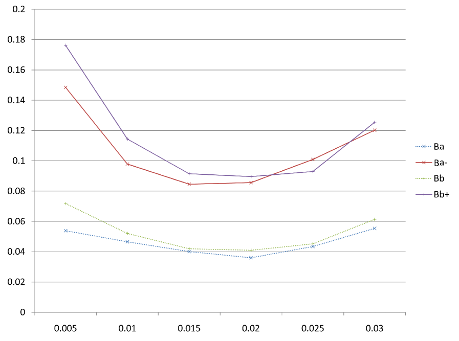
Figure 2: Plot of execution intensities estimate as a function of the spread for the stock SOGN.PA on the 18/04/2011, expressed in $s^{-1}$ (affine interpolation).

3 Optimal limit/market order strategies

3.1 Control problem formulation

Our market model in the previous section is completely determined by the state variables $(X,Y,P,S)$ controlled by the limit/marker order trading strategies $\alpha$ $\in$ ${\cal A}$.

The objective of the market maker is the following. She wants to maximize over a finite horizon $T$ the profit from her transactions in the LOB, while keeping under control her inventory (usually starting from zero), and getting rid of her inventory at the terminal date:

$$\mbox{ maximize }\;\;\;{\bf E}\big{[}U(X_{T})-\gamma\int_{0}^{T}g(Y_{t})dt\big{]}$$ (3.1)

over all limit/market order trading strategies $\alpha$ $=$ $(\alpha^{make},\alpha^{take})$ in ${\cal A}$ such that $Y_{T}$ $=$ $0$. Here $U$ is an increasing reward function, $\gamma$ is a nonnegative constant, and $g$ is a nonnegative convex function, so that the last integral term $\int_{0}^{T}g(Y_{t})dt$ penalizes the variations of the inventory. Typical frameworks include the two following cases:

$\bullet$ Mean-quadratic criterion: $U(x)$ $=$ $x$, $\gamma$ $>$ $0$, $g(y)$ $=$ $y^{2}$.

$\bullet$ Exponential utility maximization: $U(x)$ $=$ $-\exp(-\eta x)$, $\gamma$ $=$ $0$.

Let us first remove mathematically the terminal constraint on the inventory: $Y_{T}$ $=$ $0$, by introducing the liquidation function $L(x,y,p,s)$ defined on $\mathbb{R}^{2}\times\mathbb{P}\times\mathbb{S}$ by:

$$L(x,y,p,s) = x-c(-y,p,s)\;=\;x+yp-|y|\frac{s}{2}-\varepsilon.$$

This represents the value that an investor would obtained by liquidating immediately by a market order her inventory position $y$ in stock, given a cash holdings $x$, a mid-price $p$ and a spread $s$. Then, problem (3.1) is formulated equivalently as

$$\mbox{ maximize }\;\;\;{\bf E}\big{[}U(L(X_{T},Y_{T},P_{T},S_{T}))-\gamma\int_{0}^{T}g(Y_{t})dt\big{]}$$ (3.2)

over all limit/market order trading strategies $\alpha$ $=$ $(\alpha^{make},\alpha^{take})$ in ${\cal A}$. Indeed, the maximal value of problem (3.1) is clearly smaller than the one of problem (3.2) since for any $\alpha$ $\in$ ${\cal A}$ s.t. $Y_{T}$ $=$ $0$, we have $L(X_{T},Y_{T},P_{T},S_{T})$ $=$ $X_{T}$. Conversely, given an arbitrary $\alpha$ $\in$ ${\cal A}$, let us consider the control $\tilde{\alpha}$ $\in$ ${\cal A}$, coinciding with $\alpha$ up to time $T$, and to which one add at the terminal date $T$ the market order consisting in liquidating all the inventory $Y_{T}$. The associated state process $(\tilde{X},\tilde{Y},P,S)$ satisfies: $\tilde{X}_{t}$ $=$ $X_{t}$, $\tilde{Y}_{t}$ $=$ $Y_{t}$ for $t$ $<$ $T$, and $\tilde{X}_{T}$ $=$ $L(X_{T},Y_{T},P_{T},S_{T})$, $\tilde{Y}_{T}$ $=$ $0$. This shows that the maximal value of problem (3.2) is smaller and then equal to the maximal value of problem (3.1).

We then define the value function for problem (3.2) (or (3.1)):

$$v(t,z,s) = \sup_{\alpha\in{\cal A}}{\bf E}_{t,z,s}\Big{[}U(L(Z_{T},S_{T}))-\gamma\int_{t}^{T}g(Y_{u})du\Big{]}$$ (3.3)

for $t$ $\in$ $[0,T]$, $z$ $=$ $(x,y,p)$ $\in$ $\mathbb{R}^{2}\times\mathbb{P}$, $s$ $\in$ $\mathbb{S}$. Here, given $\alpha$ $\in$ ${\cal A}$, ${\bf E}_{t,z,s}$ denotes the expectation operator under which the process $(Z,S)$ $=$ $(X,Y,P,S)$ solution to (2.1)-(2.4)-(2.5)-(2.6)-(2.7), with initial state $(Z_{t^{-}},S_{t^{-}})$ $=$ $(z,s)$, is taken. Problem (3.3) is a mixed regular/impulse control problem in a regime switching jump-diffusion model, that we shall study by dynamic programming methods. Since the spread takes finite values in $\mathbb{S}$ $=$ $\delta\mathbb{I}_{m}$, it will be convenient to denote for $i$ $\in$ $\mathbb{I}_{m}$, by $v_{i}(t,z)$ $=$ $v(t,z,i\delta)$. By misuse of notation, we shall often identify the value function with the $\mathbb{R}^{m}$-valued function $v$ $=$ $(v_{i})_{i\in\mathbb{I}_{m}}$ defined on $[0,T]\times\mathbb{R}^{2}\times\mathbb{P}$.

3.2 Dynamic programming equation

For any $q$ $=$ $(q^{b},q^{a})$ $\in$ ${\cal Q}$, $\ell$ $=$ $(\ell^{b},\ell^{a})$ $\in$ $[0,\bar{\ell}]^{2}$, we consider the second-order nonlocal operator:

$${\cal L}^{q,\ell}\varphi(t,x,y,p,s) = {\cal P}\varphi(t,x,y,p,s)+R(t)\varphi(t,x,y,p,s)$$ (3.4)

$$\;+\;\lambda^{b}(q^{b},s)\big{[}\varphi(t,\Gamma^{b}(x,y,p,s,q^{b},\ell^{b}),p,s)-\varphi(t,x,y,p,s)\big{]}$$

$$\;+\;\lambda^{a}(q^{a},s)\big{[}\varphi(t,\Gamma^{a}(x,y,p,s,q^{a},\ell^{a}),p,s)-\varphi(t,x,y,p,s)\big{]},$$

for $(t,x,y,p,s)$ $\in$ $[0,T]\times\mathbb{R}^{2}\times\mathbb{P}\times\mathbb{S}$, where

$$R(t)\varphi(t,x,y,p,s) = \sum_{j=1}^{m}r_{ij}(t)\big{[}\varphi(t,x,y,p,j\delta)-\varphi(t,x,y,p,i\delta)\big{]},\;\;\;\mbox{ for }s=i\delta,\;i\in\mathbb{I}_{m},$$

and $\Gamma^{b}$ (resp. $\Gamma^{a}$) is defined from $\mathbb{R}^{2}\times\mathbb{P}\times\mathbb{S}\times{\cal Q}^{b}\times\mathbb{R}_{+}$ (resp. $\mathbb{R}^{2}\times\mathbb{P}\times\mathbb{S}\times{\cal Q}^{a}\times\mathbb{R}_{+}$ into $\mathbb{R}^{2}$) by

$$\Gamma^{b}(x,y,p,s,q^{b},\ell^{b}) = (x-\pi^{b}(q^{b},p,s)\ell^{b},y+\ell^{b})$$

$$\Gamma^{a}(x,y,p,s,q^{a},\ell^{a}) = (x+\pi^{a}(q^{a},p,s)\ell^{a},y-\ell^{a}).$$

The first term of ${\cal L}^{q,\ell}$ in (3.4) correspond to the infinitesimal generator of the diffusion mid-price process $P$, the second one is the generator of the continuous-time spread Markov chain $S$, and the two last terms correspond to the nonlocal operator induced by the jumps of the cash process $X$ and inventory process $Y$ when applying an instantaneous limit order control $(Q_{t},L_{t})$ $=$ $(q,\ell)$.

Let us also consider the impulse operator associated to market order control, and defined by

$${\cal M}\varphi(t,x,y,p,s) = \sup_{e\in[-\bar{e},\bar{e}]}\varphi(t,\Gamma^{take}(x,y,p,s,e),p,s),$$

where $\Gamma^{take}$ is the impulse transaction function defined from $\mathbb{R}^{2}\times\mathbb{P}\times\mathbb{S}\times\mathbb{R}$ into $\mathbb{R}^{2}$ by:

$$\Gamma^{take}(x,y,p,s,e) = \Big{(}x-c(e,p,s),y+e\Big{)},$$

The dynamic programming equation (DPE) associated to the control problem (3.3) is the quasi-variational inequality (QVI):

$$\min\big{[}-\displaystyle\frac{\partial v}{\partial t}-\sup_{(q,\ell)\in{\cal Q}(s)\times[0,\bar{\ell}]^{2}}{\cal L}^{q,\ell}v\;+\;\gamma g\;,\;v-{\cal M}v\big{]} = 0,\mbox{ on }[0,T)\times\mathbb{R}^{2}\times\mathbb{P}\times\mathbb{S}$$ (3.5)

together with the terminal condition:

$$v(T,x,y,p,s) = U(L(x,y,p,s)),\;\forall(x,y,p)\in\mathbb{R}^{2}\times\mathbb{P}\times\mathbb{S}.$$ (3.6)

This is also written explicitly in terms of system of QVIs for the functions $v_{i}$, $i$ $\in$ $\mathbb{I}_{m}$:

$$\min\Big{[}-\displaystyle\frac{\partial v_{i}}{\partial t}-{\cal P}v_{i}-\sum_{j=1}^{m}r_{ij}(t)[v_{j}(t,x,y,p)-v_{i}(t,x,y,p)]$$

$$\;\;\;\;\;-\;\sup_{(q^{b},\ell^{b})\in{\cal Q}_{i}^{b}\times[0,\bar{\ell}]}\lambda_{i}^{b}(q^{b})[v_{i}(t,x-\pi_{i}^{b}(q^{b},p)\ell^{b},y+\ell^{b},p)-v_{i}(t,x,y,p)]$$

$$\;\;\;\;\;-\;\sup_{(q^{a},\ell^{a})\in{\cal Q}_{i}^{a}\times[0,\bar{\ell}]}\lambda_{i}^{a}(q^{a})[v_{i}(t,x+\pi_{i}^{a}(q^{a},p)\ell^{a},y-\ell^{a},p)-v_{i}(t,x,y,p)]\;+\gamma g(y)\;;$$

$$v_{i}(t,x,y,p)-\sup_{e\in[-\bar{e},\bar{e}]}v_{i}(t,x-c_{i}(e,p),y+e,p)\Big{]} = 0,$$

for $(t,x,y,p)$ $\in$ $[0,T)\times\mathbb{R}^{2}\times\mathbb{P}$, together with the terminal condition:

$$v_{i}(T,x,y,p) = U(L_{i}(x,y,p)),\;\;\;\;\;\;\forall(x,y,p)\in\mathbb{R}^{2}\times\mathbb{P},$$

where we set $L_{i}(x,y,p)$ $=$ $L(x,y,p,i\delta)$.

By methods of dynamic programming, one can show by standard arguments that the value function $v$ is the unique viscosity solution to the QVI (3.5)-(3.6) under suitable growth conditions depending on the utility function $U$ and penalty function $g$. We next focus on some particular cases of interest for reducing remarkably the number of states variables in the dynamic programming equation DPE.

3.3 Two special cases

1. Mean criterion with penalty on inventory

We first consider the case as in [12] where:

$$U(x)\;=\;x,\;\;x\in\mathbb{R}, \mbox{ and }\;\;\;(P_{t})_{t}\;\mbox{ is a martingale}.$$ (3.7)

The martingale assumption of the stock price under the historical measure under which the market maker performs her criterion, reflects the idea that she has no information on the future direction of the stock price. Moreover, by starting typically from zero endowment in stock, and by introducing a penalty function on inventory, the market maker wants to keep an inventory that fluctuates around zero.

In this case, and exploiting similarly as in [2] the martingale property that ${\cal P}p$ $=$ $0$, we see that the solution $v$ $=$ $(v_{i})_{i\in\mathbb{I}_{m}}$ to the dynamic programming system (3.5)-(3.6) is reduced into the form:

$$v_{i}(t,x,y,p) = x+yp+\phi_{i}(t,y),$$ (3.8)

where $\phi$ $=$ $(\phi_{i})_{i\in\mathbb{I}_{m}}$ is solution the system of integro-differential equations (IDE):

$$\min\Big{[}-\displaystyle\frac{\partial\phi_{i}}{\partial t}-\sum_{j=1}^{m}r_{ij}(t)[\phi_{j}(t,y)-\phi_{i}(t,y)]$$

$$\;\;\;\;\;-\;\sup_{(q^{b},\ell^{b})\in{\cal Q}_{i}^{b}\times[0,\bar{\ell}]}\lambda_{i}^{b}(q^{b})[\phi_{i}(t,y+\ell^{b})-\phi_{i}(t,y)+\big{(}\frac{i\delta}{2}-\delta 1_{q^{b}=Bb_{+}}\big{)}\ell^{b}]$$

$$\;\;\;\;\;-\;\sup_{(q^{a},\ell^{a})\in{\cal Q}_{i}^{a}\times[0,\bar{\ell}]}\lambda_{i}^{a}(q^{a})[\phi_{i}(t,y-\ell^{a})-\phi_{i}(t,y)+\big{(}\frac{i\delta}{2}-\delta 1_{q^{a}=Ba_{-}}\big{)}\ell^{a}]\;+\gamma g(y)\;;$$

$$\phi_{i}(t,y)-\sup_{e\in[-\bar{e},\bar{e}]}[\phi_{i}(t,y+e)-\frac{i\delta}{2}|e|-\varepsilon]\Big{]} = 0,$$

together with the terminal condition:

$$\phi_{i}(T,y) = -|y|\frac{i\delta}{2}-\varepsilon,$$

These one-dimensional IDEs can be solved numerically by a standard finite-difference scheme by discretizing the time derivative of $\phi$, and the grid space in $y$. The reduced form (3.8) shows that the optimal market making strategies are price independent, and depend only on the level of inventory and of the spread, which is consistent with stylized features in the market. Actually, the IDEs for $(\phi_{i})$ even show that optimal policies do not depend on the martingale modeling of the stock price.

2. Exponential utility criterion

We next consider as in [1] a risk averse market marker:

$$U(x) = -\exp(-\eta x),\;x\in\mathbb{R},\;\eta>0,\;\;\;\gamma\;=\;0,$$ (3.9)

and assume that $P$ follows a Bachelier model:

$$dP_{t} = bdt+\sigma dW_{t}.$$

Such price process may take negative values in theory, but at the short-time horizon where high-frequency trading take place, the evolution of an arithmetic Brownian motion looks very similar to a geometric Brownian motion as in the Black-Scholes model.

In this case, we see, similarly as in [8], that the solution $v$ $=$ $(v_{i})_{i\in\mathbb{I}_{m}}$ to the dynamic programming system (3.5)-(3.6) is reduced into the form:

$$v_{i}(t,x,y,p) = U(x+yp)\varphi_{i}(t,y),$$ (3.10)

where $\varphi$ $=$ $(\varphi_{i})_{i\in\mathbb{I}_{m}}$ is solution the system of one-dimensional integro-differential equations (IDE):

$$\max\Big{[}-\displaystyle\frac{\partial\varphi_{i}}{\partial t}+(b\eta y-\frac{1}{2}\sigma^{2}(\eta y)^{2})\varphi_{i}-\sum_{j=1}^{m}r_{ij}(t)[\varphi_{j}(t,y)-\varphi_{i}(t,y)]$$

$$\;\;\;\;\;-\;\inf_{(q^{b},\ell^{b})\in{\cal Q}_{i}^{b}\times[0,\bar{\ell}]}\lambda_{i}^{b}(q^{b})[\exp\big{(}-\eta\big{(}\frac{i\delta}{2}-\delta 1_{q^{b}=Bb_{+}}\big{)}\ell^{b}\big{)}\varphi_{i}(t,y+\ell^{b})-\varphi_{i}(t,y)]$$

$$\;\;\;\;\;-\;\inf_{(q^{a},\ell^{a})\in{\cal Q}_{i}^{a}\times[0,\bar{\ell}]}\lambda_{i}^{a}(q^{a})[\exp\big{(}-\eta\big{(}\frac{i\delta}{2}-\delta 1_{q^{a}=Ba_{-}}\big{)}\ell^{a}\big{)}\varphi_{i}(t,y-\ell^{a})-\varphi_{i}(t,y)]$$

$$\varphi_{i}(t,y)-\inf_{e\in[-\bar{e},\bar{e}]}[\exp\big{(}\eta|e|\frac{i\delta}{2}+\eta\varepsilon\big{)}\varphi_{i}(t,y+e)]\Big{]} = 0,$$

together with the terminal condition:

$$\varphi_{i}(T,y) = \exp(\eta|y|\frac{i\delta}{2}).$$

Actually, we notice that the reduced form (3.10) holds more generally when $P$ is a Lévy process, by using the property that in the case: ${\cal P}U(x+yp)$ $=$ $\psi(y)U(x+yp)$ for some function $\psi$ depending on the characteristics of the generator ${\cal P}$ of the Lévy process. As in the above mean-variance criterion case, the reduced form (3.10) shows that the optimal market making strategies are price independent, and depend only on the level of inventory and of the spread. However, it depends on the model (typically the volatility) for the stock price.

4 Computational results

In this section, we provide numerical results in the case of a mean criterion with penalty on inventory, that we will denote within this section by $\alpha^{\star}$. We used parameters shown in table (4) together with transition probabilities $(\rho_{ij})_{1\leq i,j\leq M}$ calibrated in table (1) and execution intensities calibrated in table (3), slightly modified to make the bid and ask sides symmetric.

Parameter	Signification	Value
$\delta$	Tick size	0.005
$\rho$	Per share rebate	0.0008
$\epsilon$	Per share fee	0.0012
$\epsilon_{0}$	Fixed fee	$10^{-6}$
$\lambda(t)$	Tick time intensity	$\equiv 1s^{-1}$

(a) Market parameters

Parameter	Signification	Value
$U(x)$	Utility function	$x$
$\gamma$	Inventory penalization	5
$\bar{\ell}$	Max. volume make	100
$\bar{e}$	Max. volume take	100

(b) Optimization parameters

Parameter	Signification	Value
$T$	Length in seconds	300 s
$y_{min}$	Lower bound shares	-1000
$y_{max}$	Upper bound shares	1000
$n$	Number of time steps	100
$m$	Number of spreads	6

(c) Discretization/localization parameters

Parameter	Signification	Value
$N^{MC}$	Number of paths for MC simul.	$10^{5}$
$\Delta t$	Euler scheme time step	0.3 s
$\bar{\ell}_{0}$	B/A qty for bench. strat.	100
$x_{0}$	Initial cash	0
$y_{0}$	Initial shares	0
$p_{0}$	Initial price	45

(d) Backtest parameters

Table 4: Parameters

Shape of the optimal policy. The reduced form (3.8) shows that the optimal policy $\alpha^{\star}$ does only depend on time $t$, inventory $y$ and spread level $s$. One can represent $\alpha^{\star}$ as a mapping $\alpha^{\star}:\mathbb{R}^{+}\times\mathbb{R}\times\mathbb{S}\rightarrow{\cal A}$ with $\alpha^{\star}=(\alpha^{\star,make},\alpha^{\star,take})$ thus it divides the space $\mathbb{R}^{+}\times\mathbb{R}\times\mathbb{S}$ in two zones $\mathcal{M}$ and $\mathcal{T}$ so that $\alpha^{\star}_{\mid\mathcal{M}}=(\alpha^{\star,make},0)$ and $\alpha^{\star}_{\mid\mathcal{T}}=(0,\alpha^{\star,take})$. Therefore we plot the optimal policy in one plane, distinguishing the two zones by a color scale. For the zone $\mathcal{M}$, due to the complex nature of the control, which is made of four scalars, we only represent the prices regimes.

(a) near date $0$

(b) near date $T$

Figure 3: Stylized shape of the optimal policy sliced in YS.

Moreover, when using constant tick time intensity $\lambda(t)\equiv\lambda$ and in the case where $T\gg\frac{1}{\lambda}$ we can observe on numerical results that the optimal policy is mainly time invariant near date $0$; on the contrary, close to the terminal date $T$ the optimal policy has a transitory regime, in the sense that it critically depends on the time variable $t$. This matches the intuition that to ensure the terminal constraint $Y_{T}=0$, the optimal policy tends to get rid of the inventory more aggressively when close to maturity. In figure 3, we plotted a stylized view of the optimal policy, in the plane $(y,s)$, to illustrate this phenomenon.

Benchmarked empirical performance analysis. We made a backtest of the optimal strategy $\alpha^{\star}$, on simulated data, and benchmarked the results with the three following strategies:

$\bullet$ Optimal strategy without market orders (WoMO), that we denote by $\alpha^{w}$: this strategy is computed using the same IDEs, but in the case where the investor is not allowed to use market orders, which is equivalent to setting $\bar{e}=0$.

$\bullet$ Constant strategy, that we denote by $\alpha^{c}$: this strategy is the symmetric best bid, best ask strategy with constant quantity $\bar{\ell}_{0}$ on both sides, or more precisely $\alpha^{c}:=(\alpha^{c,make},0)$ with $\alpha_{t}^{c,make}\equiv(Bb,Ba,\bar{\ell}_{0},\bar{\ell}_{0})$.

$\bullet$ Random strategy, that we denote by $\alpha^{r}$: this strategy consists in choosing randomly the price of the limit orders and using constant quantities on both sides, or more precisely $\alpha^{r}:=(\alpha^{r,make},0)$ with $\alpha_{t}^{r,make}=(\varsigma_{t}^{b},\varsigma_{t}^{a},\bar{\ell}_{0},\bar{\ell}_{0})$ where $(\varsigma_{.}^{b},\varsigma_{.}^{a})$ is s.t. $\forall t\in[0;T]$ , ${\bf P}(\varsigma_{t}^{b}=Bb)={\bf P}(\varsigma_{t}^{b}=Bb_{+})={\bf P}(\varsigma_{t}^{a}=Ba)={\bf P}(\varsigma_{t}^{a}=Ba_{-})=\frac{1}{2}$.

Our backtest procedure is described as follows. For each strategy $\alpha\in\{\alpha^{\star},\alpha^{w},\alpha^{c},\alpha^{r}\}$, we simulated $N^{MC}$ paths of the tuple $(X^{\alpha},Y^{\alpha},P,S,N^{a,\alpha},N^{b,\alpha})$ on $[0,T]$, according to eq. (2.1)-(2.4)-(2.5)-(2.6)-(2.7), using a standard Euler scheme with time-step $\Delta t$. Therefore we can compute the empirical mean (resp. empirical standard deviation), that we denote by $m(.)$ (resp. $\sigma(.)$), for several quantities shown in table (5).

		optimal $\alpha^{\star}$	WoMO $\alpha^{w}$	constant $\alpha^{c}$	random $\alpha^{r}$
Terminal wealth	$m(X_{T})/\sigma(X_{T})$	2.117	1.999	0.472	0.376
	$m(X_{T})$	26.759	25.19	24.314	24.022
	$\sigma(X_{T})$	12.634	12.599	51.482	63.849
Num. of exec. at bid	$m(N^{b}_{T})$	18.770	18.766	13.758	21.545
	$\sigma(N^{b}_{T})$	3.660	3.581	3.682	4.591
Num. of exec. at ask	$m(N^{a}_{T})$	18.770	18.769	13.76	21.543
	$\sigma(N^{a}_{T})$	3.666	3.573	3.692	4.602
Num. of exec. at market	$m(N^{market}_{T})$	6.336	0	0	0
	$\sigma(N^{market}_{T})$	2.457	0	0	0
Maximum Inventory	$m(\sup_{s\in[0;T]}|Y_{s}|)$	241.019	176.204	607.913	772.361
	$\sigma(\sup_{s\in[0;T]}|Y_{s}|)$	53.452	23.675	272.631	337.403

Table 5: Performance analysis: synthesis of benchmarked backtest ($10^{5}$ simulations).

Optimal strategy $\alpha^{\star}$ demonstrates significant improvement of the information ratio $\operatorname{IR}(X_{T}):=m(X_{T})/\sigma(X_{T})$ compared to the benchmark, which is confirmed by the plot of the whole empirical distribution of $X_{T}$ (see figure (4)).

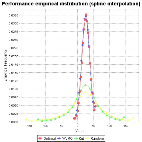
Figure 4: Empirical distribution of terminal wealth $X_{T}$ (spline interpolation).

Even if absolute values of $m(X_{T})$ are not representative of what would be the real-world performance of such strategies, these results prove that the different layers of optimization are relevant. Indeed, one can compute the ratios $\left[m(X_{T}^{\alpha^{\star}})-m(X_{T}^{\alpha^{c}})\right]/\sigma(X_{T}^{\alpha^{\star}})=0.194$ and $\left[m(X_{T}^{\alpha^{\star}})-m(X_{T}^{\alpha^{w}})\right]/\sigma(X_{T}^{\alpha^{\star}})=0.124$ that can be interpreted as the performance gain, measured in number of standard deviations, of the optimal strategy $\alpha^{\star}$ compared respectively to the constant strategy $\alpha^{c}$ and the WoMO strategy $\alpha^{w}$. Another interesting statistics is the surplus profit per trade $\left[m(X_{T}^{\alpha^{\star}})-m(X_{T}^{\alpha^{c}})\right]/\left[m(N^{b,\alpha^{\star}}_{T})+m(N^{a,\alpha^{\star}}_{T})+m(N^{market,\alpha^{\star}}_{T})\right]=0.056$ euros per trade, recalling that the maximum volume we trade is $\bar{\ell}=\bar{e}=100$. Note that for this last statistics, the profitable effects of the per share rebates $\rho$ are partially neutralized because the number of executions is comparable between $\alpha^{\star}$ and $\alpha^{c}$; therefore the surplus profit per trade is mainly due to the revenue obtained from making the spread. To give a comparison point, typical clearing fee per execution is $0.03$ euros on multilateral trading facilities, therefore, in this backtest, the surplus profit per trade was roughly twice the clearing fees.

We observe in the synthesis table that the number of executions at bid and ask are symmetric, which is also confirmed by the plots of their empirical distributions in figure (5). This is due to the symmetry in the execution intensities $\lambda^{b}$ and $\lambda^{a}$, which is reflected by the symmetry around $y=0$ in the optimal policy.

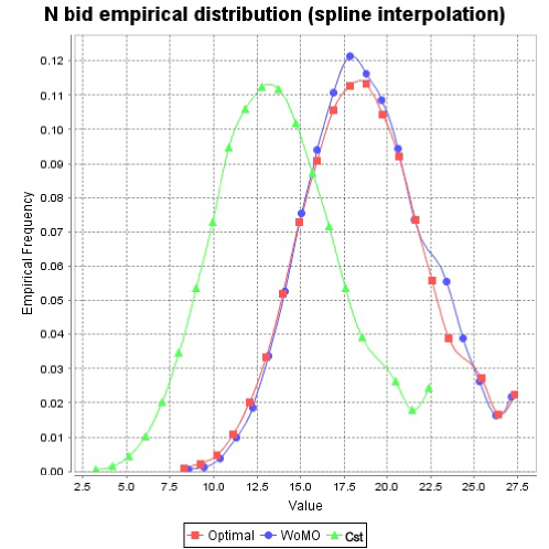
(a) N Bid empirical distribution

(b) N Ask empirical distribution

Figure 5: Empirical distribution of the number of executions on both sides.

Moreover, notice that the maximum absolute inventory is efficiently kept close to zero in $\alpha^{\star}$ and $\alpha^{w}$, whereas in $\alpha^{c}$ and $\alpha^{r}$ it can reach much higher values. The maximum absolute inventory is higher in the case of $\alpha^{\star}$ than in the case $\alpha^{w}$ due to the fact that $\alpha^{\star}$ can unwind any position immediately by using market orders, and therefore one may post higher volume for limit orders between two trading at market, profiting from reduced execution risk.

Efficient frontier. An important feature of our algorithm is that the market maker can choose the inventory penalization parameter $\gamma$. To illustrate its influence, we varied the inventory penalization $\gamma$ from $50$ to $6.10^{-2}$, and then build the efficient frontier for both the optimal strategy $\alpha^{\star}$ and for the WoMO strategy $\alpha^{w}$. Numerical results are provided in table (6) and a plot of this data is in figure (6).

$\gamma$	$\displaystyle\sigma(X_{T}^{\alpha^{\star}})$	$\displaystyle m(X_{T}^{\alpha^{\star}})$	$\displaystyle\sigma(X_{T}^{\alpha^{w}})$	$\displaystyle\sigma(X_{T}^{\alpha^{w}})$	$\operatorname{IR}(X^{\alpha^{\star}}_{T})$	$\operatorname{NIR}(X^{\alpha^{\star}}_{T})$
50.000	5.283	12.448	4.064	9.165	2.356	-2.246
25.000	7.562	18.421	7.210	16.466	2.436	-0.779
12.500	9.812	22.984	9.531	20.971	2.343	-0.135
6.250	11.852	25.932	11.749	24.232	2.188	0.136
3.125	14.546	28.153	14.485	26.752	1.935	0.263
1.563	15.819	28.901	16.830	28.234	1.827	0.289
0.781	19.088	29.952	19.593	29.145	1.569	0.295
0.391	20.898	30.372	20.927	29.728	1.453	0.289
0.195	23.342	30.811	23.247	30.076	1.320	0.278
0.098	25.232	30.901	24.075	30.236	1.225	0.261
0.049	26.495	31.020	24.668	30.434	1.171	0.253
0.024	27.124	30.901	25.060	30.393	1.139	0.242
0.012	27.697	31.053	25.246	30.498	1.121	0.243
0.006	28.065	30.998	25.457	30.434	1.105	0.238

Table 6: Efficient frontier data

We display both the “gross” information ratio $\operatorname{IR}(X^{\alpha^{\star}}_{T}):=m(X^{\alpha^{\star}}_{T})/\sigma(X^{\alpha^{\star}}_{T})$ and the “net” information ratio $\operatorname{NIR}(X^{\alpha^{\star}}_{T}):=\left(m(X^{\alpha^{\star}}_{T})-m(X^{\alpha^{c}}_{T})\right)/\sigma(X^{\alpha^{\star}}_{T})$ to have more precise interpretation of the results. Indeed, $m(X^{\alpha}_{T})$ seems largely overestimated in this simulated data backtest compared to what would be real-world performance, for all $\alpha\in\{\alpha^{\star},\alpha^{w},\alpha^{c},\alpha^{r}\}$. Then, to ease interpretation, we assume that $\alpha^{c}$ has zero mean performance in real-world conditions, and therefore offset the mean performance $m(X^{\alpha^{\star}}_{T})$ by the constant $-m(X^{\alpha^{c}}_{T})$ when computing the NIR. This has simple visual interpretation as shown in figure (6).

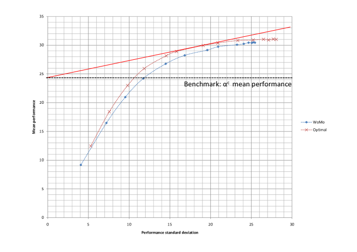
Figure 6: Efficient frontier plot

Observe that highest (net) information ratio is reached for $\gamma\simeq 0.8$ for this set of parameters. At this point $\gamma\simeq 0.8$, the annualized value of the NIR (obtained by simple extrapolation) is $47$, but this simulated data backtest must be completed by a backtest on real data. Qualitatively speaking, the effect of increasing the inventory penalization parameter $\gamma$ is to increase the zone $\mathcal{T}$ where we trade at market. This induces smaller inventory risk, due to the fact that we unwind our position when reaching relatively small values for $|y|$. This feature can be used to enforce a soft maximum inventory constraint directly by choosing $\gamma$.

References

- [1] Avellaneda M. and S. Stoikov (2008): “High frequency trading in a limit order book”, Quantitative Finance, 8(3), 217-224.
- [2] Bayraktar E. and M. Ludkovski (2011): “Liquidation in limit order books with controlled intensity”, available at: arXiv:1105.0247
- [3] Cartea A. and S. Jaimungal (2011): “Modeling Asset Prices for Algorithmic and High Frequency Trading”, preprint University of Toronto.
- [4] Cont R., Stoikov S. and R. Talreja (2010): “A stochastic model for order book dynamics”, Operations research, 58, 549-563.
- [5] Frey S. and Grammig (2008): “Liquidity supply and adverse selection in a pure limit order book market” High Frequency Financial Econometrics, Physica-Verlag HD, 83-109, J. Bauwens L., Pohlmeier W. and D. Veredas (Eds.)
- [6] Gould M.D., Porter M.A, Williams S., McDonald M., Fenn D.J. and S.D. Howison (2010): “The limit order book: a survey”, preprint.
- [7] Grillet-Aubert L. (2010): “Négociation d’actions: une revue de la littérature à l’usage des régulateurs de marché”, AMF, available at: http://www.amf-france.org/documents/general/9530_1.pdf.
- [8] Guéant O., Fernandez Tapia J. and C.-A. Lehalle (2011): “Dealing with inventory risk”, preprint.
- [9] Hendershott T., Jones C.M. and A.J. Menkveld (2010): “Does algorithmic trading improve liquidity?”, Journal of Finance, to appear.
- [10] Kühn C. and M. Stroh (2010): ”Optimal portfolios of a small investor in a limit order market: a shadow price approach”, Mathematics and Financial Economics, 3(2), 45-72.
- [11] A.J. Menkveld (2011): ”High frequency trading and the new-market makers”, preprint.
- [12] Stoikov S. and M. Saglam (2009): “Option market making under inventory risk”, Review of Derivatives Research, 12(1), 55-79.
- [13] Veraart L.A.M. (2011): ”Optimal Investment in the Foreign Exchange Market with Proportional Transaction Costs”, Quantitative Finance, 11(4): 631-640. 2011.