The Little Rip

Abstract

We examine models in which the dark energy density increases with time (so that the equation-of-state parameter $w$ satisfies $w<-1$), but $w\rightarrow-1$ asymptotically, such that there is no future singularity. We refine previous calculations to determine the conditions necessary to produce this evolution. Such models can display arbitrarily rapid expansion in the near future, leading to the destruction of all bound structures (a “little rip”). We determine observational constraints on these models and calculate the point at which the disintegration of bound structures occurs. For the same present-day value of $w$, a big rip with constant $w$ disintegrates bound structures earlier than a little rip.

I Introduction

Observations indicate that roughly 70% of the energy density in the universe is in the form of an exotic, negative-pressure component, dubbed dark energy Knop ; Riess . (See Ref. Copeland for a recent review.) If $\rho_{DE}$ and $p_{DE}$ are the density and pressure, respectively, of the dark energy, then the dark energy can be characterized by the equation-of-state parameter $w_{DE}$, defined by

$$w_{DE}=p_{DE}/\rho_{DE}.$$ (1)

It was first noted by Caldwell Caldwell that observational data do not rule out the possibility that $w_{DE}<-1$. Such “phantom” dark energy models have several peculiar properties. The density of the dark energy increases with increasing scale factor, and both the scale factor and the phantom energy density can become infinite at a finite $t$, a condition known as the “big rip” Caldwell ; rip ; Taka ; rip2 . It has even been suggested that the finite lifetime for the universe in these models may provide an explanation for the apparent coincidence between the current values of the matter density and the dark energy density doomsday .

While $w(a)<-1$ as $a$ extends into the future is a necessary condition for a future singularity, it is not sufficient. In particular, if $w$ approaches $-1$ sufficiently rapidly, then it is possible to have a model in which $\rho_{DE}$ increases with time, but in which there is no future singularity. Conditions which produce such an evolution (specified in terms of $p_{DE}$ as a function of $\rho_{DE}$) were explored in Refs. NOT ; Stefancic .

In this paper, we examine such models in more detail. In particular, we will extend the parameter space discussed in Refs. NOT ; Stefancic in both directions, showing that there are nonsingular models in which $\rho_{DE}$ increases more rapidly than the nonsingular models discussed in those references, and, conversely, that there are singular models with $\rho_{DE}$ increasing less rapidly than the singular models discussed in Refs. NOT ; Stefancic . Models without a future singularity in which $\rho_{DE}$ increases with time will nonetheless eventually lead to a dissolution of bound structures at some point in the future, a process we have dubbed the “little rip.” We discuss the time scales over which this process occurs. Finally, we consider observational constraints on these models.

In the next section, we examine the conditions necessary for a future singularity in models with $w<-1$. In Secs. III and IV, specific little-rip models and disintegration of bound systems are studied. Finally, in Sec. V, there is discussion.

II The Conditions for a Future Singularity

We limit our discussion to a spatially flat universe, for which the Friedmann equation is

$$\left(\frac{\dot{a}}{a}\right)^{2}=\frac{\rho}{3},$$ (2)

where $\rho$ is the total density, $a$ is the scale factor, the dot will always denote a time derivative, and we take $\hbar=c=8\pi G=1$ throughout. We will examine the future evolution of our universe from the point at which the pressure and density are dominated by the dark energy, so we can assume $\rho=\rho_{DE}$ and $p=p_{DE}$, and for simplicity we will drop the $DE$ subscript. Then the dark energy density evolves as

$$\dot{\rho}=-3\left(\frac{\dot{a}}{a}\right)(\rho+p).$$ (3)

The simplest way to achieve $w<-1$ is to take a scalar field Lagrangian with a negative kinetic term, and the conditions necessary for a future singularity in such models have been explored in some detail Hao ; Sami ; Faraoni ; Kujat . Here, however, we explore the more general question of the conditions under which a dark energy density that increases with time can avoid a future singularity, and the consequences of such models.

One can explore this question from a variety of starting points, by specifying, for example, the scale factor $a$ as a function of the time $t$ (an approach taken, for example, in Refs. Barrow1 ; Barrow2 ; CV ; BL ). Alternately one can specify the pressure $p$ as a function of the density $\rho$, as in Refs. NOT ; Stefancic . Note that this is equivalent to specifying the equation-of-state parameter $w$ as a function of $\rho$, since $w=p/\rho$. Finally, one can specify the density $\rho$ as a function of the scale factor $a$. Since we are interested specifically in nonsingular models for which $\rho$ increases with $a$, we shall adopt this last approach, but we will briefly examine the other two starting points. Of course, given any one of these three functions, the other two can be derived uniquely, but not always in a useful form.

For example, suppose that we specify $a(t)$. In order to avoid a big rip, it is sufficient that $a(t)$ simply be a nonsingular function for all $t$. Writing

$$a=e^{f(t)},$$ (4)

where $f(t)$ is a nonsingular function, the density is given by equation (2) as $\rho=3(\dot{a}/a)^{2}=3\dot{f}^{2}$, and the condition that $\rho$ be an increasing function of $a$ is simply $d\rho/da=(6/\dot{a})\dot{f}\ddot{f}>0$, which is satisfied as long as

$$\ddot{f}>0.$$ (5)

Thus, all little-rip models are described by an equation of the form (4), with nonsingular $f$ satisfying equation (5).

Now consider the approach of Refs. NOT ; Stefancic , who expressed the pressure as a function of the density in the form

$$p=-\rho-f(\rho),$$ (6)

where $f(\rho)>0$ ensures that the $\rho$ increases with scale factor. In order to determine the existence of a future singularity, one can integrate equation (3) to obtain NOT

$$a=a_{0}\exp\left(\int\frac{d\rho}{3f(\rho)}\right),$$ (7)

and equation (2) then gives NOT

$$t=\int\frac{d\rho}{\sqrt{3\rho}f(\rho)}.$$ (8)

The condition for a big-rip singularity is that the integral in equation (8) converges. Taking a power law for $f(\rho)$, namely

$$f(\rho)=A\rho^{\alpha},$$ (9)

we see that a future singularity can be avoided for $\alpha\leq 1/2$ NOT ; Stefancic . We examine this boundary in more detail below, noting that one can have $f(\rho)$ increase more rapidly than $\rho^{1/2}$ without a future singularity.

Now consider the third possibility: specifying the density $\rho$ as an increasing function of scale factor $a$. We will seek upper and lower bounds on the growth rate of $\rho(a)$ that can be used to determine whether or not a big-rip singularity is produced. Defining $x\equiv\ln a$, we can rewrite equation (2) as

$$t=\int\sqrt{\frac{3}{\rho(x)}}dx,$$ (10)

and the condition for avoiding a future big-rip singularity is

$$\int_{x_{0}}^{\infty}\frac{1}{\sqrt{\rho(x)}}dx\rightarrow\infty.$$ (11)

The case $p=-\rho-A\rho^{1/2}$ from Refs. NOT ; Stefancic corresponds to

$$\frac{\rho}{\rho_{0}}=\left(\frac{3A}{2\sqrt{\rho_{0}}}\ln(a/a_{0})+1\right)^{2},$$ (12)

where $w\leq-1$ requires $A\geq 0$, and we take $\rho=\rho_{0}$ and $a=a_{0}$ at a fixed time $t_{0}$. Expressing this density as a function of time rather than scale factor gives a much simpler expression:

$$\frac{\rho}{\rho_{0}}=e^{\sqrt{3}A(t-t_{0})}.$$ (13)

The equation-of-state parameter $w$ corresponding to equation (12) can be derived from the relation $(a/\rho)(d\rho/da)=-3(1+w)$:

$$w=-1-\frac{1}{\frac{3}{2}\ln(\frac{a}{a_{0}})+\frac{\sqrt{\rho_{0}}}{A}},$$ (14)

and the corresponding expansion law is

$$\frac{a}{a_{0}}=e^{(2\sqrt{\rho_{0}}/3A)[e^{(\sqrt{3}A/2)(t-t_{0})}-1]}.$$ (15)

However, we can find $\rho(a)$ for which $\rho$ increases more rapidly with $a$, but for which equation (11) is still satisfied. For example, writing $\rho^{1/2}\sim(\ln a)(\ln\ln a)$ as $a\rightarrow\infty$ satisfies equation (11). An example of such a $\rho$, with a free parameter B, is

$$\frac{\rho}{\rho_{0}}=N\left(\frac{a}{a_{0}},B\right)\frac{(1+\ln(\frac{a}{a_{0}}+B))^{2}}{(1+\ln(1+B))^{2}}\frac{(\ln(1+\ln(\frac{a}{a_{0}}+B)))^{2}}{(\ln(1+\ln(1+B)))^{2}},$$ (16)

where the choice

$$N\left(\frac{a}{a_{0}},B\right)=\frac{(\frac{a}{a_{0}}+B)^{2}}{(1+B)^{2}(\frac{a}{a_{0}})^{2}}$$ (17)

leads to a real, nonnegative $\rho$ and an analytic form for the behavior of $a(t)$:

$$\frac{a}{a_{0}}=e^{(e^{{\ln(1+\ln(1+B))e^{\left[\frac{\sqrt{\rho_{0}/3}(t-t_{0})}{(1+B)(1+\ln(1+B))\ln(1+\ln(1+B))}\right]}}}-1)}-B.$$ (18)

This argument can be extended further. In general, if we denote $\ln_{j}(x)\equiv\ln\ln\ln....\ln(x)$, where the logarithm on the right-hand side is iterated $j$ times, then any function of the form

$$\rho\sim(\ln a)^{2}(\ln_{2}a)^{2}(\ln_{3}a)^{2}...(\ln_{m}a)^{2}$$ (19)

satisfies equation (11) as $a\rightarrow\infty$ and avoids a big-rip singularity. A density increasing as in equation (19) leads to an expansion law of the form

$$a\sim\exp(\exp(\exp...(\exp(t))...)),$$ (20)

where there are $m+1$ exponentials. We have omitted the constants in equations (19) and (20) for the sake of clarity. Equation (20), while growing extraordinarily rapidly, is manifestly nonsingular. While an expansion law of this sort might seem absurd, it is probably less so than a big-rip expansion law, and in any case our goal is to try to determine the boundary between little-rip and big-rip evolution for $\rho(a)$. In this spirit, consider the slowest growing power-law modification to equation (19):

$$\rho\sim(\ln a)^{2}(\ln_{2}a)^{2}(\ln_{3}a)^{2}...(\ln_{m}a)^{2+\epsilon},$$ (21)

where $\epsilon>0$ is a constant. No matter how small $\epsilon$ is, and despite the fact that it modifies an extraordinarily slowly growing nested logarithm function, the growth law in equation (21) leads to a future big-rip singularity.

Note that the bounds specified by equations (19) and (21) are not sharp; we can always find forms for $\rho(a)$ that interpolate between these two behaviors and produce either a little rip or a big rip. However, as we take $m$ to be arbitrarily large, nearly any function of interest will increase more rapidly than equation (19) or more slowly than equation (21), allowing us a practical, if not a rigorously sharp, bound. This lack of a sharp bound is due to the fact that there is no bound on the fastest growing function $a(t)$ which is nonsingular at finite $t$.

If one is willing to place other restrictions on the form of $\rho(a)$, then more stringent bounds apply. Barrow Barrow3 demonstrated that if $\rho+3p$ is a rational function of $a$ and $t$, and $a(t)$ is nonsingular at finite $t$, then $a(t)$ can grow no more rapidly than the double exponential of a polynomial in $t$. Our equation (19) violates this condition because of the logarithmic functions.

III Constraining little-rip models

Here we shall examine in more detail the two specific little-rip models given by equations (12) and (16), which we will call model 1 and model 2, respectively. Note that we do not make use of equations (15) and (18) here, as these are valid only when the matter density can be neglected in comparison to the dark energy density. Model 1 is characterized by a single free parameter $A$, and the scale factor behaves asymptotically as a double exponential in $t$, as in equation (15):

$$a(t)\stackrel{{\scriptstyle t\rightarrow+\infty}}{{\longrightarrow}}e^{e^{t}}$$ (22)

The parameter $A$ is chosen to make a best fit to the latest supernova data from the Supernova Cosmology Project SCP , and has the best-fit value $A=3.46\times 10^{-3}{\rm Gyr}^{-1}$, while a $95\%$ C.L. fit can be found for the range $-2.74\times 10^{-3}{\rm Gyr}^{-1}\leq A\leq 9.67\times 10^{-3}{\rm Gyr}^{-1}$.

Model 2 is characterized by the free parameter $B$ and has a scale factor that behaves asymptotically as a triple exponential in $t$, as in equation (18):

$$a(t)\stackrel{{\scriptstyle t\rightarrow+\infty}}{{\longrightarrow}}e^{e^{e^{t}}}$$ (23)

The parameter $B$ is chosen to make a best fit to SCP as well, and it has the value $B=1.23$. The confidence interval for $B$ at the $95\%$ C.L. is $1.12\leq B\leq 1.34$. In fitting both models, $\Omega_{m_{0}}=0.274$, $\Omega_{x_{0}}=1-\Omega_{m_{0}}$, and $H_{0}=70.1$ km s^-1 Mpc^-1, which are consistent with the best-fit ranges for these values given by WMAP WMAP . The resultant Hubble and residual $\Lambda$CDM ($w=-1$) plots of distance modulus $\mu$ versus redshift $z$ for both models are displayed in Fig. 1.

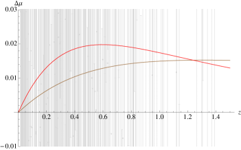
Figure 1: Top panel: Hubble plot of distance modulus $\mu$ versus redshift $z$ for the $\Lambda$CDM ($w=-1$) model (green) and models 1 (brown) and 2 (red). The lines are essentially indistinguishable. Bottom panel: The $\Lambda$CDM model is subtracted from models 1 (brown) and 2 (red). The $\Lambda$CDM model is, by definition, represented by the $\Delta\mu=0$ axis. As can be judged by the size of the error bars of the data, all are excellent fits to the supernovae data. (The color plots are in the online version of the paper.)

Not surprisingly, the best-fit models closely resemble the $\Lambda$CDM model, which is known to be an excellent fit to the data Melchiorri . To see this more clearly, note that our models will resemble a cosmological constant at low redshift as long as $\rho(a)\sim constant$ for $a\sim a_{0}$. For model 1, this condition is satisfied when $A/\sqrt{\rho_{0}}\ll 1$ in equation (12), while for model 2, we require $B\simeq 1.39$ in equation (16). To see that $B$ should be close to this value, one should expand equation (16) around $a=a_{0}$. The zeroth-order term is $\rho_{0}$, and the coefficient for the first-order term is $0$ when $B=1.39$. A comparison with our best-fit values indicates that these conditions are, indeed, satisfied. Furthermore, in the limit where these conditions are satisfied, these little-rip models closely resemble, at low redshift, big-rip models close to $\Lambda$CDM, i.e., models with constant $w<-1$ and $|1+w|\ll 1$. To see this, recall that constant-$w$ big-rip models have a density varying with scale factor as

$$\rho=\rho_{0}(a/a_{0})^{-3(1+w)}.$$ (24)

For $|1+w|\ll 1$ and $a/a_{0}$ not too far from 1, equation (24) behaves as

$$\rho\approx\rho_{0}[1-3(1+w)\ln(a/a_{0})].$$ (25)

Equation (12) reduces to equation (25) for $A/\sqrt{\rho_{0}}\ll 1$, with $A/\sqrt{\rho_{0}}=-(1+w)$.

IV Disintegration

A feature of a big rip is that all bound-state systems disintegrate before the final singularity rip . Here we show that little-rip models, despite not having a final singularity, also produce the disintegration of bound structures. As a first approximation, the disintegration time is when the dark energy density equals the mean density of the system. A more accurate method was presented in rip2 . We shall employ both methods to estimate the disintegration of the Sun-Earth system. For the little-rip models 1 and 2, with the best-fit parameters derived in the previous section, we find the time $t_{\odot-\oplus}$ from the present time $t_{0}$ until the Earth ($\oplus$) - Sun ($\odot$) system is disintegrated to be:

$${\bf{\rm Model~{}1:}}~{}~{}~{}~{}~{}~{}t_{\odot-\oplus}\simeq 8~{}{\rm Tyrs}$$ (26)

$${\bf{\rm Model~{}2:}}~{}~{}~{}~{}~{}~{}t_{\odot-\oplus}\simeq 146~{}{\rm Gyrs}.$$ (27)

Note that the disintegration time for model 2 is less than that of model 1, which is expected since $\rho$ for model 2 grows faster than $\rho$ for model 1.

It is straightforward to estimate the corresponding $t_{\odot-\oplus}$ for big-rip models with constant $w$ to be Taka

$$t_{\odot-\oplus}\simeq\left(\frac{11~{}{\rm Gyrs}}{|1+w|}\right),$$ (28)

and it is almost identical to $t_{rip}$, which is about one year later.

Clearly, little-rip models can produce this disintegration either earlier or later than big-rip models, depending on the exact parameters of each model. For example, by putting, $w=-1-10^{-3}$ in equation (28), we find a value of $11$ Tyrs for $t_{\odot-\oplus}$, which is larger than that of models 1 and 2 in Eqs.(26, 27). In this case, disintegration occurs earlier in the little-rip model than in the big-rip model.

The five energy conditions (weak, null, dominant, null dominant, strong) (see, e.g., Ref. Carroll ) are all violated by all little-rip and big-rip models. A simple way to see this is that if $w<-1$, which occurs for any rip, a boost is allowed with $(v/c)^{2}>-w/c$ to an inertial frame with negative energy density. Having said that, if general relativity itself fails for length scales bigger than that of galaxies, we may not be constrained by the same energy conditions.

V Discussion

In the big rip, the scale factor and density diverge in a singularity at a finite future time. In the $\Lambda$CDM model, there is no such divergence and no disintegration because the dark energy density remains constant. The little rip interpolates between these two cases; mathematically it can be represented as an infinite limit sequence which has the big rip and the $\Lambda$CDM model as its boundaries. Such models can be represented generically by a density varying with scale factor as in equation (19).

Physically, in the little rip, the scale factor and the density are never infinite at a finite time. Nevertheless, such models generically lead to structure disintegration at a finite time. For models consistent with current supernova observations, such disintegration can occur either earlier or later in a little-rip model than in a big-rip model, depending on the parameters chosen for the models. However, for a given present-day value of $w$, the big-rip model with constant $w$ will necessarily lead to an earlier disintegration than the little-rip model with the same present-day value of $w$. This results from the fact that $w$ increases monotonically in the little rip models, resulting in a smaller value for $\rho$ at any given $a$ than in the corresponding constant-$w$ big-rip model, and therefore, a lower expansion rate. Thus, supernova bounds on the epoch of disintegration for constant-$w$ big-rip models also apply to little-rip models; one cannot simultaneously satisfy supernova constraints and hasten the onset of disintegration to an arbitrarily early time simply by iterating exponentials in the expansion law.

Furthermore, supernova data force both big-rip and little-rip models into a region of parameter space in which both models resemble $\Lambda$CDM. In this limit, big-rip and little-rip models produce essentially the same expansion law up to the present, despite having very different future evolution. Thus, current data already make it essentially impossible to determine whether or not the universe will end in a future singularity.

Finally, we remark that since the novel and speculative cyclic cosmology proposed in Ref. BF requires only disintegration and not a singularity, such cyclicity would seem to be possible within a little-rip model instead of the big rip considered in BF . This is one potentially fruitful direction for future research FLS2 .

- (1) R.A. Knop, et al., Ap.J. 598, 102 (2003).
- (2) A.G. Riess, et al., Ap.J. 607, 665 (2004).
- (3) E.J. Copeland, M. Sami, and S. Tsujikawa, Int. J. Mod. Phys. D 15, 1753 (2006).
- (4) R.R. Caldwell, Phys. Lett. B 545, 23 (2002).
- (5) R.R. Caldwell, M. Kamionkowski, and N.N. Weinberg, Phys. Rev. Lett. 91, 071301 (2003).
- (6) P.H. Frampton and T. Takahashi, Phys. Lett. B 557, 135 (2003).
- (7) S. Nesseris and L. Perivolaropoulos, Phys. Rev. D70, 123529 (2004).
- (8) R.J. Scherrer, Phys. Rev. D71, 063519 (2005).
- (9) S. Nojiri, S.D. Odintsov, and S. Tsujikawa, Phys. Rev. D71, 063004 (2005); S. Nojiri and S.D. Odintsov, Phys. Rev. D72, 023003 (2005).
- (10) H. Stefancic, Phys. Rev. D71, 084024 (2005).
- (11) J.-G. Hao and X.-Z. Li, Phys. Rev. D70, 043529 (2004).
- (12) M. Sami and A. Toporensky, Mod. Phys. Lett. A 19, 1509 (2004).
- (13) V. Faraoni, Class. Quant. Grav. 22, 3235 (2005).
- (14) J. Kujat, R.J. Scherrer, and A.A. Sen, Phys. Rev. D74, 083501 (2006).
- (15) J.D. Barrow, Class. Quant. Grav. 21, L79 (2004).
- (16) J.D. Barrow, Class. Quant. Grav. 21, 5619 (2004).
- (17) C. Cattoen and M. Visser, Class. Quant. Grav. 22, 4913 (2005).
- (18) J.D. Barrow and S.Z.W. Lip, Phys. Rev. D80, 043518 (2009).
- (19) J.D. Barrow, Class. Quant. Grav. 13, 2965 (1996).
- (20) R. Amanullah, et al. (The Supernova Cosmology Project) Ap.J, 716, 712-738 (2010).
- (21) E. Komatsu et al., Ap.J. 192, 18 (2011).
- (22) P. Serra, A. Cooray, D.E. Holz, A. Melchiorri, S. Pandolfi, and D. Sarkar, Phys. Rev. D80, 121302 (2009).
- (23) K.P. Schröder and R.C. Smith, Mon. Not. Royal Astron. Soc. 386, 155 (2008).
- (24) S.M. Carroll, M. Hoffmann and M. Trodden, Phys. Rev. D68, 023509 (2003).
- (25) L. Baum and P.H. Frampton, Phys Rev. Lett. 98, 071301 (2007).
- (26) P.H. Frampton, K.J. Ludwick and R.J. Scherrer, in preparation.