Theoretical Aspects of the Fractional Quantum Hall Effect in Graphene

Abstract

We review the theoretical basis and understanding of electronic interactions in graphene Landau levels, in the limit of strong correlations. This limit occurs when inter-Landau-level excitations may be omitted because they belong to a high-energy sector, whereas the low-energy excitations only involve the same level, such that the kinetic energy (of the Landau level) is an unimportant constant. Two prominent effects emerge in this limit of strong electronic correlations: generalised quantum Hall ferromagnetic states that profit from the approximate four-fold spin-valley degeneracy of graphene’s Landau levels and the fractional quantum Hall effect. Here, we discuss these effects in the framework of an SU(4)-symmetric theory, in comparison with available experimental observations.

I Introduction

The theory of non-interacting massless Dirac fermions in two spatial dimensions provides the framework which allows for the understanding of most of graphene’s low-energy electronic properties.antonioRev At first sight, this may seem astonishing because the Coulomb interaction is strictly speaking of an intermediate strength; indeed, within a typical Coulomb-gas argument, one compares the average interaction energy $e^{2}k_{F}/\epsilon$, at the characteristic length $\sim k_{F}^{-1}$, in terms of the Fermi wave vector $k_{F}$ and the dielectric constant $\epsilon$ of the environment surrounding the graphene sheet, to the kinetic energy $\hbar v_{F}k_{F}$ at the same length scale. The ratio between these energies yields the coupling constant $\alpha_{G}=e^{2}/\hbar\epsilon v_{F}\simeq 2/\epsilon$, which is reminiscent of the fine-structure constant in quantum electrodynamics if one replaces the speed of light $c$ by the Fermi velocity $v_{F}$, i.e. the characteristic velocity of the electrons in a material. Because $v_{F}\simeq c/300$ in graphene, the graphene fine-structure constant $\alpha_{G}$ is roughly 300 times larger than that ($\alpha=1/137$) of quantum electrodynamics.

In view of the rather large coupling constant, one might expect to see correlation effects in graphene, which happen though to be sparse.kotov Indeed, electronic instabilities are not only triggered by the (bare) coupling constant, but one also needs to take into account the density of states at the Fermi level in the discussion of such instabilities.mahan ; GV As a consequence of the linearity and the two-dimensional (2D) character of graphene electrons, the density of states, however, vanishes linearly with the Fermi energy when approaching the limit of undoped (intrinsic) graphene, such that electronic instabilities are suppressed. In the search of prominent correlation effects, one should therefore investigate situations in which the density of states in graphene is enhanced. A (logarithmically) diverging density of states is typically encountered at van Hove singularities due to saddle points in the band dispersion. Van Hove singularities occur at extremely high energies ($\sim 3$ eV) in monolayer graphene and are thus inaccessible with the help of field-effect doping. In contrast to monolayer graphene, they occur at rather small energies in AB-stacked bilayer graphene ($\sim 3$ meV), MF06 which are only resolved at electronic densities below $10^{11}~{}\text{cm}^{-2}$. A promising system in this respect is twisted bilayer graphene, where van Hove singularities at intermediate energies ($\sim 10...100$ meV) have been observed. vanHoveTwist Such twists naturally occur in epitaxial graphene grown on the carbon face of the SiC crystal.deheer

An alternative means of inducing a large density of states in graphene, and thus of increasing the role of electronic correlations, is to expose the sample to a strong perpendicular magnetic field $B$. In this case the electronic energy is quantised into highly degenerate Landau levels (LLs) at discrete energies $E_{n}$, around which the density of states $\rho(E)$ is strongly peaked, $\rho(E)=gn_{B}\sum_{n}f(E-E_{n})$, where $n_{B}=eB/h$ is the flux density measured in units of the flux quantum $h/e$ and $g$ takes into account internal degrees of freedom, such as the four-fold spin-valley degeneracy ($g=4$) in graphene. The functions $f(E-E_{n})$, which are normalised to one, $\int dE\,f(E-E_{n})=1$, become delta functions in the clean limit, which we assume in the theoretical discussion here. Each LL may thus be viewed, in this limit, as an infinitely flat energy band the density of states of which grows linearly with the magnetic field.

In this article, we review some effects due to the magnetic-field induced electronic correlations in graphene, in comparison with the perhaps better-known 2D electron gas in semiconductor heterostructures. The probably most prominent one is the fractional quantum Hall effect (FQHE), which has recently been observed experimentally in the two-terminaldu09 ; bolotin09 and the four-terminal configuration.ghahari10 ; dean10 In contrast to the FQHE in GaAs heterostructures, the graphene FQHE reflects a four-component structuretoke07 ; GR07 that is inherited from the four-fold spin-valley degeneracy and that goes along with particular magnetic properties described in the framework of SU(4) quantum Hall ferromagnetism.goerbigRev The latter is also relevant in the discussion of interaction-induced integer quantum Hall effects (IQHE) at integer filling factors $\nu$ that do not belong to the “magic” series $\nu=n_{el}/n_{B}=\pm 2,\pm 6,\pm 10,...$, in terms of the carrier density $n_{el}$.

The article is organised as follows. In Sec. II, we review some of the experimental findings from the observations of the IQHE in 2005 to the very recent ones of the FQHE in the four-terminal geometry, in 2010. After an introduction to the theoretical basics of graphene LLs in Sec. III, we discuss the SU(4)-spin-valley quantum Hall ferromagnetism in Sec. III.1 and the SU(4) theory of the FQHE in Sec. III.2.

II Experimental Situation

II.1 Relativistic integer quantum Hall effect

A milestone experiment in graphene research was the observation in 2005 of a particular – relativistic – IQHE in graphene, when changing either the electronic density via the electric-field effect at a fixed magnetic field or when varying the field at fixed electronic density.novoselov05 ; zhang05 The samples used in these magnetotransport measurements were obtained with the help of the exfoliation technique,exfol and the effect has later (in 2009) been confirmed in epitaxial graphene samples,epitaxIQHE which have also been proven to be promising for metrological means because of a high-precision (with an error bar on the order of $10^{9}$) Hall-resistance quantisation.tza Whereas the effect has the same signature – a plateau in the Hall resistance accompanied by a vanishing longitudinal resistance – as that in conventional 2D electron systems, it occurs at unusual filling factors,

$$\nu=\pm 2(2n+1)=\pm 2,\pm 6,\pm 10,...,$$ (1)

and reflects the relativistic nature of the charge carriers in graphene. Indeed, the two possible signs $\pm$ reflect the presence of a conduction band ($+$ for “particles”) that touches the valence band ($-$ for “anti-particles” on the hole-doped side). The filling-factor steps in units of four between successive plateaus may easily be understood as a consequence of the four-fold spin-valley degeneracy, which was not resolved in these first experiments and that yields four copies of each LL. The offset of $\pm 2$ in the plateau series (1) is a consequence of relativistic LL quantisation that yields a LL spectrum

$$E_{\lambda,n}=\hbar\frac{v_{F}}{l_{B}}\sqrt{2n},$$ (2)

where $l_{B}=\sqrt{\hbar/eB}\simeq 26/\sqrt{B\text{[T]}}$ nm is the magnetic length, and the integers $n$ label the levels in the conduction band ($\lambda=+$) or in the valence band ($\lambda=-$). The most prominent feature of the level spectrum (2), apart from its square-root dispersion with the magnetic field and with $n$, is the presence of a zero-energy LL for $n=0$. It is this level that is responsible for the offset $\pm 2$ in the series (1) because it is only half-filled at zero doping, $\nu=0$. This means that the condition for the IQHE, namely a set of completely filled LLs with a topmost filled level separated by a gap from the lowest unoccupied LL, is not fulfilled at $\nu=0$, but only at $\nu=2$ (for electron doping) or $\nu=-2$ (for hole doping), as a consequence of the four-fold spin-valley degeneracy of the $n=0$ LL.

II.2 Additional plateaus at integer fillings

In 2006, one year after the discovery of the graphene IQHE, novel high-field plateaus have been observed at $\nu=0,\pm 1$ and $\pm 4$ that do not belong to the series (1).zhang06 These additional states indicate that the spin-valley degeneracy in the $n=0$ LL is completely lifted, whereas in $n=1$ it is only partially lifted – if it were fully lifted in the latter case, one would also expect an IQHE at $\nu=\pm 3$ and $\pm 5$. The explanations which have been given for the spin-valley degeneracy lifting fall into two classes: (1) extrinsic or (2) intrinsic, i.e. interaction-induced, effects. The simplest extrinsic effect is certainly the Zeeman effect that would lift the spin degeneracy, such that each four-fold degenerate LL is split into two (valley-degenerate) spin branches separated by an energy scale of $\Delta_{Z}\simeq 1.2B\text{[T]}$ K. A more subtle extrinsic effect, as a consequence of electron-phonon coupling, is capable of lifting the valley degeneracy in the zero-energy LL in form of the generation of a mass gap in the level spectrum.FL ; nomura09 ; mudry10 The coupling to an out-of-plane phonon can yield a Peierls-type distortion and can thus break the inversion symmetry of the lattice.FL More recently an inplane Kekulé distortion has been investigated that couples the two different valleys.nomura09 ; mudry10 In contrast to the out-of-plane distortion, the latter mechanism yields a mass term (and thus a valley splitting) that does not depend on the coupling to the substrate and that has been evaluated to be roughly $\Delta_{kek}\simeq 2B\text{[T]}$ K. Notice that the linear $B$-field dependence simply reflects the fact that the coupling is proportional to the density of states $\rho(E)\propto B$, which scales linearly with the magnetic field, as mentioned in the introduction.

The second class of degeneracy-lifting effects contains mechanisms that are triggered by the Coulomb interaction between the electrons and that are discussed in more detail in Sec. III.1. One effect is the so-called magnetic catalysis, which has been investigated before the discovery of the IQHE in graphene, in the context of Dirac fermions.khvesh01 The mechanism consists of a mass-gap generation that yields the same level spectrum (and thus a valley-degeneracy lifting) as that due to the above-mentioned Peierls-type distortions, but it is dynamically generated by the electron-electron interactions themselves.khvesh01 ; Mcata The mass term plays the role of an order parameter that has been identified with exciton condensation. Independently, quantum-Hall ferromagnetism, both in the spin and in the valley channel, has been proposed in 2006 as a possible route to understanding the additional plateaus.nomura06 ; GMD ; AF06 ; YDSMD06 Quantum-Hall ferromagnetism is an exchange effect, where the electron-electron interaction is minimised by the formation of a maximally antisymmetric orbital wave function, accompanied by a maximally symmetric valley-spin part. The effect is particularly efficient in LLs because the latter may be viewed as infinitely flat bands – the polarisation of the spin and the valley pseudospin is therefore not accompanied by a cost in kinetic energy. Whereas quantum-Hall ferromagnetism is capable of generating a transport gap, and thus an IQHE, at all integer filling factors that do not belong to the series (1),arovas a mass gap resulting from a lattice distortion or magnetic catalysis can only lift the valley degeneracy in the zero-energy LL $n=0$. However in both cases, magnetic catalysis and quantum-Hall ferromagnetism, the gap scales with the typical interaction energy $e^{2}/\epsilon l_{B}\propto\sqrt{B}$.

energy	value for arbitrary $B$	for $B=25$ T
$\Delta_{Z}$	$1.2B{\rm[T]}$ K	$30$ K
$\Delta_{kek}$	$2B{\rm[T]}$ K	$50$ K
$e^{2}/\varepsilon l_{B}$ (vacuum)	$139\sqrt{B{\rm[T]}}$ K	$694$ K
$e^{2}/\varepsilon l_{B}$ (on SiO2)	$104\sqrt{B{\rm[T]}}$ K	$521$ K
$e^{2}/\varepsilon l_{B}$ (on h-BN)	$109\sqrt{B{\rm[T]}}$ K	$543$ K
$e^{2}/\varepsilon l_{B}$ (on SiC)	$71\sqrt{B{\rm[T]}}$ K	$355$ K

Table 1: Tab. I. Energy scales for spin-valley degeneracy lifting in graphene LLs. The first two lines show the energy scales associated with extrinsic effects (Zeeman effect and Kekulé-type lattice distortion, $\Delta_{Z}$ and $\Delta_{kek}$, respectively), which are proportional to $B$. Below are shown the interaction-energy scales ($\propto\sqrt{B}$), different substrates taking into account both the dielectric constant of the substrate and RPA contributions from inter-band processes.

The discussed energy scales are summarised in the table above. The interaction energy scales depend on the dielectric constant $\epsilon$ of the environment, which consists in a typical experimental situation on the substrate [SiO₂, hexa boron nitride (h-BN) or SiC for epitaxial graphene] on one side and air (vacuum) on the other one. The third line (vacuum) indicates the energy scale for freestanding graphene. A recent theoretical study proposes to engineer the short-range part of interaction potential via a partial screening with a dielectric medium at a finite distance from the graphene sheet.Princeton Notice that in all cases, we have taken into account screening due to the completely filled valence band, which yields $\varepsilon=\epsilon(1+\pi\alpha_{G}/2)$ within the random-phase approximation.GGV One notices from these energy scales that in all cases the Coulomb interaction sets the leading energy scale and should thus be considered first in the discussion of the spin-valley degeneracy lifting, whereas extrinsic effects are subordinate. As it is discussed below in Sec. III.1, the extrinsic effects are cooperative with quantum-Hall ferromagnetism in the sense that they orient the interaction-induced spin-valley magnetisation in a particular direction.

II.3 Fractional quantum Hall effect in graphene

In the previous subsection, we have argued that the appearance of IQHE plateaus, which do not match the series (1), could in principle be understood without invoking electron-electron interactions – extrinsic effects could be responsible for these plateaus, although this is unlikely in view of the different energy scales involved. Clear evidence for interaction-induced phases in graphene LLs has been found in 2009 with the first observations of the FQHE at $\nu=1/3$ in suspended graphene.du09 ; bolotin09 One notices that it took roughly twice as long in graphene between the observation of the IQHE and the FQHE as compared to conventional 2D electron systems, where the IQHE was observed in 1980,KvK whereas the FQHE was discovered in 1982.TSG The necessary mobility increase of graphene samples, which is required for the observation of the FQHE, could already be achieved in 2008 in current-annealed suspended samples, where mobilities in the $100\,000~{}\text{cm}^{2}/\text{Vs}$ range have been reported.du08 However, it turned out to be an experimental challenge to obtain samples with working and sufficiently separated electronic contacts.

The above-mentioned transport measurements, which revealed the FQHE, were indeed performed in the two-terminal configuration, where the same contacts used as source and drain serve for the resistance measurement. It is therefore not possible to perform simultaneously a measurement of the longitudinal and the Hall resistance, but both are superposed, and sophisticated conformal mappings are necessary to separate the two components.ConfMap However, because of the vanishing longitudinal component in the case of the FQHE, the two-terminal resistance is then determined by the quantised “Hall” resistance and therefore reveals the characteristic plateau.

These first observations have since been confirmed in the more robust four-terminal configuration, which allows for a simultaneous measurement of and thus a clear distinction between the longitudinal and the Hall resistances. Two experiments were reported in 2010, one in a suspended graphene sampleghahari10 and another one in graphene on an h-BN substratedean10 that allows for a mobility increase upon current annealing that is in the same range as (though somewhat lower than) that in suspended graphene.dean10a In Ref. ghahari10, the activation gap could be determined and agrees rather well with that $0.05...0.1e^{2}/\varepsilon l_{B}\sim 7...14\sqrt{B{\rm[T]}}$ K one expectsAC06 ; toke06 for the polarised Laughlin state at $\nu=1/3$.laughlin In graphene on a h-BN substrate, most members of the $1/3$ FQHE family in $n=0$ (at $\nu=\pm 1/3,\pm 2/3$, and $\pm 4/3$) and all in $n=1$ (at $\nu=\pm 7/3,\pm 8/3,\pm 10/3$, and $\pm 11/3$) could be resolved to great accuracy.dean10 Whereas the absence or relative weakness of the $\pm 5/3$ member of the $1/3$-family in the zero-energy LL remains to be understood, it clearly corroborates the approximate SU(4) symmetry due to the four-fold spin-valley degeneracy underlying the FQHE in graphene,toke07 ; GR07 as discussed in more detail from the theoretical point of view in Sec. III.2. Another relevant finding in graphene on an h-BN substrate is that of additional IQHE plateaus at $\nu=\pm 3$ and $\pm 5$,dean10 which indicate a full spin-valley degeneracy lifting not only in $n=0$ but also in $n=1$. Whereas these additional plateaus cannot be explained in the framework of a mass-gap generation, either by a lattice distortion or interaction-induced magnetic catalysis, it is expected from the formation of quantum-Hall ferromagnetic states, as mentioned above.

III Theoretical Understanding

From the theoretical point of view, both the FQHE and quantum-Hall ferromagnetism require three essential ingredients: (1) infinitely flat and highly-degenerate energy bands (here in the form of LLs the degeneracy of which is characterised by the flux density $n_{B}$); (2) the Aharonov-Bohm effect, which yields a geometric phase to paths in the 2D plane and that induces the so-called magnetic translation group; and (3) sufficiently short-range interactions.

In order to make transparent the above statements, we consider a single LL that is sufficiently well separated in energy from its adjacent levels. This condition is fulfilled when the LL spacing $\Delta_{n}=\sqrt{2}\hbar(v_{F}/l_{B})(\sqrt{n+1}-\sqrt{n})\simeq\hbar v_{F}/\sqrt{2n}l_{B}\simeq 200\sqrt{B\text{[T]}/n}$ K is larger than the impurity broadening of the levels. Furthermore, because this energy scale is much larger than the extrinsic spin-valley symmetry-breaking effects (see Tab. I), we may consider each LL as four-fold degenerate, in addition to the orbital degeneracy given by the flux density $n_{B}$. The electron-electron interactions may then be separated into a low-energy and a high-energy part. The latter consists of interaction-induced inter-LL transitions at the characteristic energy scale $\Delta_{n}$, whereas the low-energy part consists of intra-LL excitations, in which case the kinetic energy (set by the scale $\hbar v_{F}/l_{B}$) effectively drops out of the problem. The low-energy interaction Hamiltonian (in reciprocal space) may then be written as

$$H_{n}=\frac{1}{2}\sum_{{\bf q}}v(q)\rho_{n}(-{\bf q})\rho_{n}({\bf q}),$$ (3)

where $v(q)=2\pi e^{2}/\varepsilon q$ is the Fourier-transformed Coulomb interaction potential, and the Fourier components of the density operator $\rho_{n}({\bf q})$ take into account only states within the $n$-th LL. Apart from a form factor $\mathcal{F}_{n}(q)$ that takes into account the overlap between electronic wave functions in the $n$-th LL and that may be absorbed into an effective interaction potential,goerbigRev the (projected) density operator

$$\bar{\rho}({\bf q})\equiv\frac{\rho_{n}({\bf q})}{\mathcal{F}_{n}({\bf q})}=\sum_{j=1}^{N}e^{-i{\bf q}\cdot{\bf R}_{j}},$$ (4)

is a sum of the one-particle density operators $\bar{\rho}_{j}({\bf q})=\exp(-i{\bf q}\cdot{\bf R}_{j})$ for each of the $N$ electrons in the $n$-th LL. Here, ${\bf R}_{j}=(X_{j},Y_{j})$ is the operator that describes the centre of the cyclotron motion (called guiding centre) of the $j$-th electron. Because it is a constant of motion, it does not connect states in different LLs, in agreement with the construction of the model (3). Furthermore, the components of ${\bf R}_{j}$ do not commute,

$$[X_{j},Y_{j^{\prime}}]=il_{B}^{2}\delta_{j,j^{\prime}},$$ (5)

which is a manifestation of the above-mentioned Aharonov-Bohm effect. Indeed, one sees from the commutation relations that $X_{j}$ and $Y_{j}$ are conjugate variables, such that $X_{j}$ generates a translation in the $-y$-direction, whereas $Y_{j}$ generates one in the $x$-direction. As a consequence the electron, when moving on a closed path around an area $\Sigma$, picks up an Aharonov-Bohm phase $\varphi=\Sigma/l_{B}^{2}=2\pi\phi/\phi_{0}$, where $\phi=B\Sigma$ is the flux in the area $\Sigma$. The commutation relations (5) furthermore induce the commutation relations

$$[\bar{\rho}({\bf q}),\bar{\rho}({\bf k})]=2i\sin\left(\frac{q_{x}k_{y}-q_{y}k_{x}}{2}l_{B}^{2}\right)\bar{\rho}({\bf q}+{\bf k})$$ (6)

for the projected density operators, such that their Heisenberg equations of motion $i\hbar\dot{\bar{\rho}}({\bf q})=[\bar{\rho}({\bf q}),H]$ become highly non-linear.

Another consequence of the commutation relations (5), which allow for the introduction of harmonic-oscillator ladder operators $b_{j}=(X_{j}+iY_{j})/\sqrt{2}l_{B}$ and $b_{j}^{\dagger}=(X_{j}-iY_{j})/\sqrt{2}l_{B}$, with $[b_{j},b_{j^{\prime}}^{\dagger}]=\delta_{j,j^{\prime}}$, is the representation of $n=0$-LL states in terms of analytic functions

$$\phi_{m}(z_{j},z_{j}^{*})\sim\left(b_{j}^{\dagger}\right)^{m}e^{-|z_{j}|^{2}/4}\sim z_{j}^{m}e^{-|z_{j}|^{2}/4},$$ (7)

where we have defined the complex position $z_{j}=(x_{j}-iy_{j})/l_{B}$ of the $j$-th particle in the 2D plane and where we have omitted the normalisation constant in the expressions. Whereas this statement is, strictly speaking, true only in the $n=0$ LL, one may nevertheless use a representation of states in other LLs in terms of analytic functions if one interprets $v_{n}(q)=v(q)|\mathcal{F}_{n}(q)|^{2}$ as an effective interaction potential that mimics the $n$-th LL while considering the projected density $\bar{\rho}({\bf q})$ as one of $n=0$. This assumption is justified by the fact that the commutation relations (6) do not explicitly depend on the LL index.

To summarise this theoretical introduction of the model, one notices the following important points.

• The above arguments are valid for any type of Landau quantisation and not restricted to the relativistic one in graphene. From this point of view, graphene and its FQHE are not so different from the FQHE in semiconductor heterostrucures.

• The specificity of graphene and relativistic LL quantisation is revealed rather in the form factors $\mathcal{F}_{n}(q)$, which take into account the wave function overlaps in a particular LL $n$ and that happen to be different from that in non-relativistic 2D electron systems, as a consequence of the spinorial structure of the electronic wave functions in graphene.

• Another specificity of graphene is its four-fold spin-valley degeneracy. The Coulomb interaction naturally commutes with the electronic spin, whereas this is a priori not the case for the valley pseudospin – indeed, the two different valleys can be coupled by scattering due to short-range components of the Coulomb potential. However, one may show that this inter-valley coupling is suppressed by a factor of $a/l_{B}\sim 0.005\sqrt{B\text{[T]}}$ because of the reciprocal-space distance $\sim a^{-1}$ between the two valleys,GMD ; AF06 such that the Coulomb interaction in graphene LLs may be viewed as approximately SU(4)-symmetric.

• A general $N$-particle wave function in graphene LLs must therefore be described by an analytic polynomial in all particle coordinates $z_{k}^{(j)}$, where the superscript $(j)$ indicates one of the four-spin valley components $(K,\uparrow)$, $(K,\downarrow)$, $(K^{\prime},\uparrow)$, or $(K^{\prime},\downarrow)$.

III.1 Interaction-induced integer quantum Hall effect

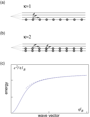
Figure 1: Spin-valley waves (Goldstone modes) in graphene LLs. (a) For one filled spin-valley subbranch ($\kappa=1$), there are three Goldstone modes connecting the filled subbranch with the empty ones. (b) For two filled subbranches ($\kappa=2$), four Goldstone modes connect the completely filled subbranches with the empty ones. (c) Dispersion relation of the spin-valley waves (continuous line). At $ql_{B}\ll 1$, the energy disperses as $E_{{\bf q}}\propto q^{2}$, as one expects for magnons. At $ql_{B}\gg 1$, the dispersion relation saturates and may be approximated by the energy to create a well-separated electron-hole pair, with a Coulomb attraction between the electron and the hole, $E_{{\bf q}}\sim[2\sqrt{\pi/8}-1/ql_{B}]e^{2}/\epsilon l_{B}$ (dashed line).

A first manifestation, the understanding of which turns out to be instructive also for the FQHE, of Coulomb interactions in graphene LLs is the formation of SU(4) quantum-Hall ferromagnetic states at integer filling factors that do not correspond to completely filled LLs described by the series (1). As already mentioned above, a repulsive interaction such as the Coulomb potential favours orbital wave functions with nodes when two particles approach each other. These nodes are naturally built in in the usual Slater determinants for $\kappa$ completely filled spin-valley branches of the last (partially) occupied LL,

$$|{\rm FM}\rangle=\prod_{j=1}^{\kappa}\prod_{m=0}^{N_{B}-1}c_{m,j}^{\dagger}|{\rm vac}\rangle,$$ (8)

where $c_{m,i}^{\dagger}$ creates an electron in the component $j$ in the state corresponding to the LL wave function $z^{m}$ and $|{\rm vac}\rangle$ denotes the fermion vacuum. For illustration, we consider the state (8) in the zero-energy LL $n=0$ and omit the LL index at the fermion operators, keeping in mind that the generalisation to other LLs is straight-forward, as discussed above.

Naturally, the state (8) is the ground state of a model with no interactions if the filled states have a lower one-particle energy than the empty ones, for example in the presence of a Zeeman effect. Here, however, we consider these effects to be absent, and we do therefore not specify whether the occupied branches are particular spin or valley states. The state (8) therefore breaks the SU(4) spin-valley symmetry, which is respected by the interaction model. As a consequence of this symmetry breaking, the quantum-Hall ferromagnet (8) has low-energy excitations in form of Goldstone modes the energy of which vanishes in the small-wave-vector limit. These Goldstone modes are spin-valley waves that connect the different possible ground states, which are obtained by relabeling the occupied subbranches. They are depicted in Fig. 1 for $\kappa=1$ (a) and $\kappa=2$ (b) completely filled subbranches – the case of $\kappa=3$ filled subbranches is particle-hole-symmetric to $\kappa=1$. For $\kappa=1$, the Goldstone modes are three-fold degenerate [see Fig. 1(a)] whereas for $\kappa=2$ there are four different types [Fig. 1(b)].

III.1.1 Spin-valley waves

The different spin-valley waves may be obtained by application of the operator

$$\bar{\rho}_{ij}({\bf q})=\sum_{m,m^{\prime}}\left\langle m\left|e^{-i{\bf q}\cdot{\bf R}}\right|m^{\prime}\right\rangle c_{m,i}^{\dagger}c_{m^{\prime},j}$$ (9)

on the state $|{\rm FM}\rangle$, where ${\bf R}$ is the one-particle operator associated with the guiding centre, as discussed above, and $j$ denotes an occupied spin-valley component, whereas $i$ corresponds to an unoccupied one. The state $\bar{\rho}_{ij}({\bf q})|{\rm FM}\rangle$ may also be viewed as a superposition of particle-hole excitations, where ${\bf q}$ is the wave vector of the excitation. As a consequence of the magnetic translation algebra, generated by the commutation relations (5), this wave vector is proportional to the distance $\Delta{\bf R}={\bf R}-{\bf R}^{\prime}$ between the guiding centre ${\bf R}$ of the electron and that ${\bf R}^{\prime}$ of the hole,

$${\bf q}=\Delta{\bf R}\times{\bf e}_{z}/l_{B}^{2}.$$ (10)

The energy spectrum of the spin-valley waves may be obtained by evaluating the Hamiltonian (3) in the state $\bar{\rho}_{ij}({\bf q})|{\rm FM}\rangle$, and one obtains

$$E_{{\bf q}} = \langle{\rm FM}|\bar{\rho}_{ij}(-{\bf q})H_{n}\bar{\rho}_{ij}({\bf q})-H_{n}|{\rm FM}\rangle$$ (11)

$$= 2\sum_{{\bf k}}v_{n}({\bf k})\sin^{2}\left(\frac{q_{x}k_{y}-k_{x}q_{y}}{2}l_{B}^{2}\right),$$

or explicitly, in the zero-energy LL $n=0$,AF06 ; YDSMD06 ; KH ; doretto

$$E_{{\bf q}}=\sqrt{\frac{\pi}{2}}\frac{e^{2}}{\epsilon l_{B}}\left[1-e^{-q^{2}l_{B}^{2}/4}I_{0}\left(\frac{q^{2}l_{B}^{2}}{4}\right)\right],$$ (12)

which is plotted in Fig. 1(c). In the last expression, which is independent of the number $\kappa$ of filled spin-valley branches and which thus indicates that the spin-valley waves are degenerate for all values of ${\bf q}$, $I_{0}(x)$ is a modified Bessel function. The limits of the dispersion (12) are transparent; for small values of the wave vector $ql_{B}\ll 1$, one obtains the usual $q^{2}$ dispersion expected for spin-wave-type modes,

$$E_{q\rightarrow 0}=\frac{\rho_{s}}{2}q^{2}l_{B}^{2},$$ (13)

in terms of the spin stiffness

$$\rho_{s}=\frac{1}{4\pi}\sum_{{\bf k}}v_{0}({\bf k})|{\bf k}|^{2}l_{B}^{2}=\frac{1}{16\sqrt{2\pi}}\frac{e^{2}}{\epsilon l_{B}}.$$ (14)

In the opposite limit, the dispersion may be understood in terms of the energy of a spatially well-separated electron-hole pair. The energy to add an electron (or a hole) to the state (8) is just given by the exchange energy, $E_{x}=\sqrt{\pi/8}(e^{2}/\epsilon l_{B})$. The value at which the dispersion (12) saturates is indeed twice the exchange energy. Furthermore, the electron and the hole with opposite charge interact via the Coulomb attraction

$$\frac{e^{2}}{\epsilon|\Delta{\bf R}|}=\frac{e^{2}}{\epsilon ql_{B}^{2}},$$ (15)

as a consequence of the connection (10) between the wave vector and the distance between the guiding centre of the electron and that of the hole. As depicted by the dashed line in Fig. 1(c), the spin-valley-wave dispersion is well approximated by the sum of these two terms,

$$E_{ql_{B}\gg 1}\simeq\left[2\sqrt{\frac{\pi}{8}}-\frac{1}{ql_{B}}\right]\frac{e^{2}}{\epsilon l_{B}}.$$ (16)

To summarise the picture of SU(4) quantum Hall ferromagnetism and the associated spin-valley-wave modes, we first mention that the polarised state (8) may be obtained simply as a consequence of the Coulomb repulsion between the electrons without the need of explicit spin-valley symmetry-breaking terms, such as the Zeeman effect. The state is stable because the dispersion of the collective excitations is gapped for any non-zero value of the wave vector, and the addition of an electron (or a hole) is associated with an energy cost given by the exchange energy, which is much larger than the external symmetry-breaking fields (see Table 1). The role of such external terms is then reduced to a simple orientation of the interaction-induced spin-valley magnetisation, similarly to a usual (spin) ferromagnet placed into a magnetic field that orients its magnetisation in the direction of the field.

In the following paragraph, we argue that there are lower-energy elementary excitations, in form of skyrmions, than such additional electron with a flipped spin or valley-pseudospin. However, their energy is also determined by the interaction-energy scale $e^{2}/\epsilon l_{B}$, such that the overall picture remains unaltered.

III.1.2 SU(4) skyrmions

In the previous paragraph, we have considered the elementary excitation to be a simple additional electron (or hole) that is added into an unoccupied spin-valley component in the quantum-Hall ferromagnet (8). Its energy is then simply given by the exchange energy $E_{x}=\sqrt{\pi/8}(e^{2}/\epsilon l_{B})$. However, it turns out to be energetically favourable for this additional particle to be dressed by a local deformation of the SU(4)-ferromagnetic background, such as to lower the energy cost due to the opposite spin orientation of the particle with respect to the background. This dressed particle is called skyrmion and carries a topological charge in addition to its electric one. For a simple SU(2) spin ferromagnet, this topological charge may be viewed as the number of times the (normalised) local magnetisation wraps, when exploring the 2D plane, the Bloch sphere the points of which represent the orientation of the magnetisation. The SU(4) spin-valley case is more complicated and requires the introduction of two additional Bloch spheres (one for the valley-pseudospin and one for the two angles that describe the entanglement between the spin and the valley-pseudospin),DGLM but the picture is essentially the same.

The topological charge $Q_{top}$, which is a positive or negative integer, determines the energy of the skyrmion excitation,sondhi ; moon

$$E_{sk}=4\pi\rho_{s}|Q_{top}|=\frac{1}{2}\sqrt{\frac{\pi}{8}}\frac{e^{2}}{\epsilon l_{B}}|Q_{top}|$$ (17)

in terms of the spin stiffness (14). One thus notices that the energy to create a skyrmion with charge $Q_{top}=\pm 1$ is half of that to create a simple (undressed) electron in an unoccupied spin-valley component. Dressing this additional electron by a topological spin-valley texture therefore lowers the energy in $n=0$ by a factor of 2. The energy gain is less in the LLs $n\neq 0$, but it remains positive for $n=1$ and $n=2$, whereas in even higher LLs it is no longer energetically favourable to dress the additional charge by creating skyrmions.toke06 ; YDSMD06

We finally mention that the skyrmion is generically larger in size than an undressed electronic excitation ($\sim l_{B}$). The size of the skyrmion is indeed determined by a competition between the Coulomb (exchange) interaction, which favours large skyrmions to maintain locally the ferromagnetic order, and external symmetry-breaking terms that, even if they are small, have a tendency to lower the number of reversed spins or valley-pseudospins and thus to lower the skyrmion size. Indeed, the skyrmion radius scales assondhi ; moon

$$\xi\sim\sqrt{\frac{e^{2}/\epsilon l_{B}}{\Delta}}l_{B},$$ (18)

where $\Delta$ represents a generic spin-valley symmetry-breaking terms, such as the Zeeman effect or that arising from a spontaneous lattice distortion discussed in Sec. II.2.

III.2 SU(4) fractional quantum Hall effect

In the previous section, we have argued that electron-electron interactions are responsible for the formation of additional plateaus at integer filling factors that do not correspond to the series (1), as a consequence of the formation of maximally polarised quantum-Hall ferromagnetic states. These considerations turn out to be helpful also in the understanding of the four-component FQHE. If we consider, e.g., the SU(4) ferromagnetic state at $\nu=\pm 1$, its orbital wave function may be written in terms of the completely anti-symmetric Slater determinant

$$\phi\left(\left\{z_{k}\right\}\right)=\prod_{k<l}^{N}\left(z_{k}-z_{l}\right)e^{-\sum_{k=1}^{N}|z_{k}|^{2}/2},$$ (19)

in terms of the complex coordinates $z_{k}$ of the electron in units of $l_{B}$, regardless of the spin-valley component they belong to. As a consequence of the anti-symmetry of this orbital wave function, the associated spin-valley wave function must be completely symmetric, i.e. precisely ferromagnetic, such as to fulfil the anti-symmetry requirement for fermionic $N$-particle wave functions. Wave function (19) is the simplest example of Laughlin’s wave functionlaughlin

$$\phi_{m}^{L}\left(\left\{z_{k}\right\}\right)=\prod_{k<l}^{N}\left(z_{k}-z_{l}\right)^{m}e^{-\sum_{k=1}^{N}|z_{k}|^{2}/2},$$ (20)

which describes FQHE states at filling factors $\nu=1/m$. Indeed, a power counting of the terms in the polynomial indicates that the largest power of an arbitrarily chosen particle component $z_{k}$ is $M=m(N-1)$. As we have already mentioned in the first part of this section, this power is delimited by the number of flux quanta threading the 2D system, such that $M=N_{B}-1$, and one obtains, in the thermodynamic limit, the relation

$$m=\frac{N_{B}}{N}=\frac{n_{B}}{n_{el}}=\frac{1}{\nu},$$ (21)

i.e. the exponent $m$ in Laughlin’s wave function determines the filling factor. For odd values of $m$ – remember from the previous discussion that $m$ must be an integer to match the analyticity condition for wave functions in the LL $n=0$ – the same symmetry arguments apply as for the wave function (19). It is a fully anti-symmetric orbital wave function, and the spin-valley part must therefore be completely symmetric, such that Laughlin’s wave function (20) represents a fully polarised spin-valley ferromagnet.

Similarly to Laughlin’s wave function, the theory of composite fermions (CF)jain89 can be extended to include the SU(4) internal degree of freedom.toke07 Still, the main physical consequences of this additional symmetry can be captured within the simpler framework of Halperin wave functions.halperin Such states have been introduced in 1983, soon after Laughlin’s original work, to take into account the electronic spin and to describe non-fully polarized FQHE states. This set of wave functions is readily generalised to the four-component case in grapheneGR07

$$\psi_{m_{1},...,m_{4};n_{ij}}^{{\rm SU}(4)}=\phi_{m_{1},...,m_{4}}^{L}\phi_{n_{ij}}^{inter},$$ (22)

in terms of the product

$$\phi_{m_{1},...,m_{4}}^{L}=\prod_{j=1}^{4}\prod_{k_{j}<l_{j}}^{N_{j}}\left(z_{k_{j}}^{(j)}-z_{l_{j}}^{(j)}\right)^{m_{j}}e^{-\sum_{j=1}^{4}\sum_{k_{j}=1}^{N_{j}}|z_{k_{j}}^{(j)}|^{2}/4}$$ (23)

of Laughlin wave functions for the four spin-valley components and the term

$$\phi_{n_{ij}}^{inter}=\prod_{i<j}^{4}\prod_{k_{i}}^{N_{i}}\prod_{k_{j}}^{N_{j}}\left(z_{k_{i}}^{(i)}-z_{k_{j}}^{(j)}\right)^{n_{ij}},$$ (24)

which describes inter-component correlations. Here, $z_{k_{j}}^{(j)}$ is the complex coordinate of a particle in the component $j$, and $N_{j}$ is the total number of $j$-type particles. As in the case of Laughlin’s wave function, the power-counting argument relates the exponents $m_{j}$ and $n_{ij}$ to the component filling factors $\nu_{j}=N_{j}/N_{B}$. Indeed, for an arbitrarily chosen component $j$, the maximal exponent is

$$N_{B}-1=m_{j}(N_{j}-1)+n_{ij}N_{i\neq j}.$$ (25)

One notices that the inter-component correlations induce additional zeros in the wave function; this is energetically favourable because the SU(4)-symmetric Coulomb interaction is as strong between particles of the same component as between those belonging to different ones. Furthermore, one notices that Eq. (25) has the character of a matrix equation, and it turns out to be useful to introduce the exponent matrix $\mathcal{M}=n_{ij}$ the diagonal elements of which are simply the intra-component exponents $n_{jj}\equiv m_{j}$ and the off-diagonal ones those corresponding to inter-component correlations. In terms of this exponent matrix, the relation between the component filling factors and the exponents reads

$$\left(\begin{array}[]{c}\nu_{1}\\ \nu_{2}\\ \nu_{3}\\ \nu_{4}\end{array}\right)=\mathcal{M}^{-1}\left(\begin{array}[]{c}1\\ 1\\ 1\\ 1\end{array}\right).$$ (26)

In the zero-energy LL, the total filling factor is related to the component filling factors by

$$\nu=-2+\sum_{j}^{4}\nu_{j},$$ (27)

as a consequence of its half-filling for $\nu=0$, whereas in all other LLs $n$ the filling factor reads

$$\nu=\pm[4(n-1)+2]+\sum_{j}^{4}\nu_{j}.$$ (28)

Notice that a state at a filling factor $\nu$ is related to another one at $-\nu$ by particle-hole symmetry.

In addition to the determination of the component filling factors, the exponent matrix $\mathcal{M}$ is useful also in two other respects. First, it allows one to distiguish between potential physical states and those that cannot describe a homogeneous liquid state that displays the FQHE. Indeed, the matrix must be positive definite, i.e. contain only positive (or zero) eigenvalues, unless the corresponding state is unstable and undergoes a phase separation between the different components.DGRG Second, The matrix $\mathcal{M}$ encodes prominent properties of the quasiparticle excitations, such as their fractional charge and their statistics.WZ Finally, the rank of the matrix $\mathcal{M}$ encodes the SU(4)-ferromagnetic properties of the different states.GR07 In order to illustrate this point, we first mention that Eq. (26) is only well-defined if $\mathcal{M}$ is invertible (of rank 4). This means that all component filling factors are fixed, and thus also all polarisations which are simple combinations of these factors; e.g. the spin polarisation (in the $z$-direction) is simply given by $S_{z}=(N/2)(\nu_{\uparrow,K}+\nu_{\uparrow,K^{\prime}}-\nu_{\downarrow,K}-\nu_{\downarrow,K^{\prime}})$, whereas the valley-pseudospin polarisation reads $P_{z}=(N/2)(\nu_{\uparrow,K}-\nu_{\uparrow,K^{\prime}}+\nu_{\downarrow,K}-\nu_{\downarrow,K^{\prime}})$. As an example, one may invoke the state with $m_{j}=3$ for all $j$ and $n_{ij}=2$ for all $i\neq j$.toke07 All component filling factors are fixed to be $\nu_{j}=1/9$, as may be seen from Eq. (26), and this state would be an SU(4)-singlet candidate for a (yet unobserved) FQHE at $\nu=-2+4/9$.

In the opposite limit, where $\mathcal{M}$ is of rank 1, the component filling factors are fully undetermined – the only combination that is fixed is the total sum. This is precisely the case of Laughlin’s wave function, which may be described as a four-component Halperin wave function (22) with all $n_{ij}=m_{j}=m$ being the same odd integer. As we have already mentioned, this corresponds to a fully polarised SU(4)-ferromagnetic state, and the sum of component filling factors is just $\sum_{j}^{4}\nu_{j}=1/m$.

There are intermediate states for which, e.g., only one of the polarisations is fixed. As an example, we may consider the state with $m_{j}=3$, $n_{12}=n_{14}=n_{23}=n_{34}=3$, and $n_{13}=n_{24}=2$, which is described by an exponent matrix of rank 2. In addition to the total filling factor, which is fixed at $\nu=-2+2/5$, the combinations $\nu_{1}+\nu_{3}=1/5$ and $\nu_{2}+\nu_{4}=1/5$ are fixed. If we identify, for illustration reasons, the components as $\{1,2,3,4\}=\{(\uparrow,K),(\uparrow,K^{\prime}),(\downarrow,K),(\downarrow,K^{\prime})\}$, this state would correspond to a valley-pseudospin singlet, with $\nu_{K}=\nu_{(\uparrow,K)}+\nu_{(\downarrow,K)}=1/5$, $\nu_{K^{\prime}}=\nu_{(\uparrow,K^{\prime})}+\nu_{(\downarrow,K^{\prime})}=1/5$, such that $P_{z}=(N/2)(\nu_{K}-\nu_{K^{\prime}})=0$, whereas the spin is polarised and free to be oriented, e.g. by an external Zeeman effect.

Interestingly, the 2/5 and 4/9 states discussed above are in competition with completely polarised CF states, that may occur at filling factors $\nu=-2+p/(2p+1)$, in terms of the integers $p$. Notice that the Halperin-type states at $2/5$ and $4/9$, which we discuss here, may alternatively be viewed as unpolarised CF states.toke07 Numerical calculations have shown that the polarised states are generally higher in energy in the zero-energy graphene LL,toke07 but they may become competitive when external symmetry-breaking terms are taken into account, such that one may expect similar spin transistions at fixed filling factors as in 2D electron systems in GaAs heterostructures.2_5spinExp Quite generally, it is important to stress that the polarisation may change drastically when varying the filling factor – even if the LL degeneracy may be lifted in a precise hierarchy at the integer filling factors $\nu=0$ and $\nu=\pm 1$, this hierarchy is easily destroyed when shifting the filling factor away from these values, as a consequence of the dominant Coulomb interaction. From a theoretical point one therefore expects that a fully spin-valley polarised state at $\nu=-2+1/3$ is depolarised when increasing the filling factor – this depolarisation is very efficient because of the low-energy skyrmion excitations of the SU(4) ferromagnetism associated with the Laughlin state. Indeed, upon increase of $\nu$ one obtains a state at $\nu=-2+2/5$ that is polarised in only one of the channels, e.g the spin for a Zeeman effect in the absence of valley-symmetry breaking terms. Upon further increase, the spin-valley polarisation disappears completely at $\nu=-2+4/9$, where an SU(4) singlet is the state of lowest energy, in the absence of extrinsic symmetry-breaking effects. However, when approaching the filling factor $\nu=-1$, the SU(4) spin-valley polarisation is again expected to be fully restored.

We emphasise that, apart from the above-mentioned states at $\nu=2/5$ and $4/9$, most of the Halperin states (22) are not eigenstates of the SU(4) symmetry group and thus not of the bare SU(4)-symmetric Coulomb interaction. However, as we discuss in the following subsection for some of such states, they can be stabilised with the help of relatively weak symmetry-breaking terms. We finally notice that this picture and the expected polarisation of the discussed FQHE states also holds true, within numerical calculations, fo the LL $n=1$.toke07

III.2.1 The 1/3 family of FQHE states

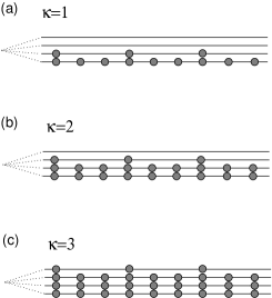
Figure 2: Sketch of different states $\psi_{\nu=-2+\kappa+1/3}$ of the 1/3 family, for (a) $\kappa=1$, (b) $\kappa=2$, and (c) $\kappa=3$.

We have discussed, until now, the use of Halperin wave functions for potential FQHE states in the filling-factor range $-2<\nu<-1$. Notice, however, the the only $n=0$ FQHE states that have been clearly identified ar $\nu=\pm 1/3,\pm 2/3$, and $\pm 4/3$, whereas the states at $\nu=\pm 5/3$ are absent or extremely weak.du09 ; bolotin09 ; ghahari10 ; dean10 The understanding of these states requires the inclusion of fully occupied spin-valley subbranches in addition to partially filled ones. In principle, these states may also be described in terms of generalised Halperin wave functions with broken SU(4) symmetry, and we terminate this review with a brief discussion of them. The states, which are depicted in Fig. 2, may be constructed by the wave functions

$$\psi_{\nu=-2+\kappa+1/3}=\prod_{j}^{\kappa}\prod_{k_{j}<l_{j}}^{N_{B}}\left(z_{k_{j}}^{(j)}-z_{l_{j}}^{(j)}\right)\prod_{k<l}^{N_{B}/3}\left(w_{k}-w_{l}\right)^{3},$$ (29)

where $z_{k_{j}}^{(j)}$ are the complex coordinates of $j$-type particles that reside in the $\kappa$ fully occupied spin-valley branches $j=1,...,\kappa$ (since $\nu_{j}=1$, we have $N_{j}=N_{B}$), whereas $w_{k}$ is that of a particle in the other spin-valley branches, occupied by $N_{B}/3$ particles, where we do not specify explicitly the component. This state is described by an exponent matrix with $m_{j}=1$ for $j=1,...,\kappa$, $m_{j}=3$ for $j=\kappa+1,...,4$, $n_{ij}=0$ if one of the indices is $1,...,\kappa$ and $n_{ij}=3$ otherwise. In the framework of quantum Hall ferromagnetism, the state may be viewed as $\kappa$ “inert” levels, whereas the electrons in the $4-\kappa$ partially occupied subbranches form a Laughlin-type state with incorporated SU($4-\kappa$) ferromagnetic low-energy excitations in terms of $(3-\kappa)$-fold degenerated spin-valley waves. Other members of the 1/3 family may be obtained from the states (29) with the help of a particle-hole transformation.

As discussed in the previous section, the states (29) cannot describe the ground state of the Coulomb interaction because they are no eigenstates of the SU(4) symmetry. These states may be stabilised artificially by a particular choice of the interaction potential between the different particles that explicitly breaks the SU(4) symmetry.papic10 However, the more physical approach which we adopt here shows that the states (29) may be relevant even for an SU(4)-symmetric interaction potential as soon as the extrinsic symmetry-breaking terms are included.

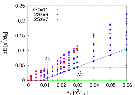
Figure 3: Energy spectrum obtained in Ref. papic10, by exact diagonalisation of $N=17$ electrons interacting via the Coulomb interaction on a sphere threaded by $N_{B}=6$ flux quanta. The spectrum is shown as a function of the Zeeman effect, in units of $e^{2}/\epsilon l_{B}$. The colours indicate levels with the different spin polarisations $S_{z}=11/2$ (green, corresponding to the state $\psi_{1/3}$) $9/2$ (blue) adn $7/2$ (pink). Red dot correspond to energy levels with other polarisation.

For $\kappa=2$ [see Fig. 2(b)], i.e. for a filling factor $\nu=1/3$, the energy spectrum obtained from exact diagonalisation is shown in Fig. 3 as a function of an extrinsic symmetry-breaking field that has been chosen to be the Zeeman effect. The spectrum has been obtained with the help of the DiagHamDiagHam code with implemented SU(4) symmetry for up to $N=17$ electrons on a sphere threaded by $N_{B}=6$ flux quanta. As expected from the above discussion, the ground state in the absence of a Zeeman effect is not the state $\psi_{\nu=1/3}$ described by Eq. (29) because it does not have the correct spin polarisation. However, the state is stabilised already for very small symmetry breaking, i.e. for a Zeeman effect above $\Delta_{Z}^{1}\simeq 0.01e^{2}/\epsilon l_{B}$, as may be seen in Fig. 3, where the ground state has the correct (maximal) spin polarisation $S_{z}=11/2$ (green dots). Although the state $\psi_{\nu=1/3}$ is the ground state above this critical value of the Zeeman effect, its low-energy excitations are not the usual collective excitations of the Laughlin state, but coherent spin-flip excitations in the sector $S_{z}=9/2$ that are represented by the blue line in Fig. 3. These spin-flip excatiations are the relevant modes below a second critical Zeeman field $\Delta_{Z}^{2}\simeq 0.03e^{2}/\epsilon l_{B}$, whereas above $\Delta_{Z}^{2}$ the lowest-energy excitations are the usual charge excitations in the same polarisation sector.

The case $\kappa=1$, which corresponds to a single fully occupied spin-valley branch [see Fig. 2(a)], may be checked within a simplified two-component scheme that neglects the two-fold degenerate spin-valley modes associated with the partially filled three subbranches $j=2$, 3 and 4. The corresponding (simplified) wave function reads

$$\psi_{\nu=-1+1/3}^{\rm 2-comp}=\prod_{k<l}^{N_{B}}\left(z_{k}-z_{l}\right)\prod_{k<l}^{N_{B}/3}\left(w_{k}-w_{l}\right)^{3},$$ (30)

where $z_{k}$ is the position of a particle in the fully occupied subbranch and $w_{k}$ one in the 1/3-filled second component. This wave function has been tested in exact-diagonalisation calculations with the help of the DiagHam codeDiagHam with an implemented SU(2)-symmetric Coulomb potential, for $N=22$ electrons on a sphere with $N_{B}=15$ flux quanta.papic10 The obtained energy spectrum shows the same features as that depicted in Fig. 3 obtained within a four-component calculation, with a similar critical field $\Delta_{Z}^{1}\simeq 0.01e^{2}/\epsilon l_{B}$ above which the state (30) is stabilised albeit with a slightly larger field $\Delta_{Z}^{2}\simeq 0.08e^{2}/\epsilon l_{B}$, below which the collective excitations are dominated by spin-flip excitations.papic10

These two results obtained numerically, for $\kappa=2$ and for $\kappa=1$ in a simplified version, hint at a certain universality in the mechanism of stabilising states of the form (29) by weak extrinsic symmetry-breaking fields. The physical picture that emerges from it may be summarised as follows: the systems has an interaction-driven tendency to form such states (here the states $\psi_{\nu=-2+\kappa+1/3}$ of the 1/3 family), but a small extrinsic SU(4) spin-valley symmetry breaking is nevertheless necessary to stabilise them. This needs to be contrasted to the SU(4) quantum Hall ferromagnetism discussed in Sec. III.1 where the state remains stable even in the complete absence of extrinsic symmetry-breaking effects.

We finally notice that, even in the intermediate regime $\Delta_{Z}^{1}<\Delta_{Z}<\Delta_{Z}^{2}$, the lowest-energy excitations in the limit $ql_{B}\gg 1$ are not the collective spin-flip excitations, but as for the usual Laughlin 1/3 state quasi-particle excitations that may eventually be dressed by SU($4-\kappa$) spin-valley textures in the partially occupied subbranches and that are responsible for the activation gap measured in the experiments.ghahari10 ; dean10

IV Conclusions

In conclusion, we have reviewed theoretically the role of electronic interactions in graphene Landau levels. These interactions are responsible for two prominent effects: (a) the formation of SU(4) spin-valley quantum Hall ferromagnets that are likely to be responsible for the observed IQHE at $\nu=0$, $\pm 1$, $\pm 3$, $\pm 4$, and $\pm 5$ that do not belong to the series (1) of the usual (relativistic) graphene IQHE; and (b) the recently observed FQHE. Although both effects are known also in the context of non-relativistic quantum Hall systems, such as in GaAs heterostructures, they are different in graphene as a consequence of the approximate SU(4) spin-valley symmetry of the Coulomb interaction potential. Even if the SU(4) symmetry of graphene LLs is broken by extrinsic effects, such as the Zeeman effect or a valley-pseudospin Zeeman-type effect due to static lattice distortions in graphene, the latter effects are associated with energy scales that are much smaller than the leading Coulomb interaction scale, for physically accessible magnetic fields. These extrinsic effects are mainly cooperative with the tendency of forming maximally spin-valley polarised states. In the context of quantum Hall ferromagnetism, they orient the preformed spin-valley magnetisation into particular channels, whereas they are necessary to stabilise the trial states $\psi_{\nu=-2+\kappa+1/3}$ that may account for the experimentally observed members of the 1/3 family.

Also other FQHE states than those of the above-mentioned 1/3 family may be described in the framework of the SU(4) theory of the FQHE and are expected to display very special spin-valley polarisations. It remains an experimental challenge to have access to these states and their physical properties, but from an experimental point of view we seem to be only at the beginning of the discovery of the possibly very rich physical properties of the graphene FQHE. The expected findings of novel FQHE states in graphene may provide other surprises that will certainly also challenge the SU(4) theory of the graphene FQHE.

References

- (1) A. H. Castro Neto, F. Guinea, N. M. R. Peres, K. S. Novoselov, and A. K. Geim, Rev. Mod. Phys. 81, 109 (2009).
- (2) V. N. Kotov, B. Uchoa, V. M. Peirera, A. H. Castro Neto, and F. Guinea, arXiv:1012.3484.
- (3) G. D. Mahan, Many-Particle Physics, Plenum Press, 2nd Ed., New York (1993).
- (4) G. F. Giuliani and G. Vignale, Quantum Theory of Electron Liquids, Cambridge UP, Cambridge (2005).
- (5) E. McCann and V. I. Fal’ko, Phys. Rev. Lett. 96, 086805 (2006).
- (6) G. Li et al., Nature Physics 6, 109 (2010).
- (7) C. Berger, Z. Song, T. Li, A. Y. Ogbazghi, R. Feng, Z. Dai, A. N. Marchenkov, E. H. Conrad, P. N. First, and W. A. de Heer, J. Phys. Chem. 108, 19912 (2004); for a recent review on epitaxial graphene, see W. A. de Heer, C. Berger, X. Wu, M. Sprinkle, Y. Hu, M. Ruan, J. A. Stroscio, P. N. First, R. Haddon, B. Piot, C. Faugeras, M. Potemski, and J.-S. Moon, J. Phys. D: Appl. Phys. 43, 374007 (2010).
- (8) X. Du, I. Skachko, F. Duerr, A. Luican, and E. Y. Andrei, Nature 462, 192 (2009).
- (9) K. I. Bolotin, F. Ghahari, M. D. Shulman, H. L. Stormer, and P. Kim, Nature 462, 196 (2009).
- (10) F. Ghahari, Y. Zhao, P. Cadden-Zimansky, K. Bolotin, P. Kim, Phys. Rev. Lett. 106, 046801 (2011)
- (11) C.R. Dean, A.F. Young, P. Cadden-Zimansky, L. Wang, H. Ren, K. Watanabe, T. Taniguchi, P. Kim, J. Hone, and K.L. Shepard, Nature Phys. 7, 693 (2011).
- (12) M. O. Goerbig and N. Regnault, Phys. Rev. B 75, 241405 (2007).
- (13) C. Töke and J. K. Jain, Phys. Rev. B 75, 245440 (2007); Z. Papić, M. O. Goerbig, and N. Regnault, Solid State Comm. 149, 1056 (2009).
- (14) For a review, see M. O. Goerbig, Rev. Mod. Phys. 83, 1193 (2011).
- (15) K. S. Novoselov, A. K. Geim, S. V. Morosov, D. Jiang, M. I. Katsnelson, I. V. Grigorieva, S. V. Dubonos, and A. A. Firsov, Nature 438, 197 (2005).
- (16) Y. Zhang, Y.-W. Tan, H. L. Stormer, and P. Kim, Nature 438 201, (2005).
- (17) K. S. Novoselov, A. K. Geim, S. V. Morosov, D. Jiang, Y. Zhang, S. V. Dubonos, I. V. Grigorieva, and A. A. Firsov, Science 306, 666 (2004); K. S. Novoselov, D. Jiang, T. Booth, V. V. Khotkevich, S. M. Morozov, and A. K. Geim, PNAS 102, 10451 (2005).
- (18) J. Jobst, D. Waldmann, F. Speck, R. Hirner, D. K. Maude, T. Seyller, and H. B. Weber, Phys. Rev. B 81, 195434 (2010); T. Shen, J. J. Gu, M. Xu, Y. Q. Wu, M. L. Bolen, M. A. Capano, L. W. Engel, and P. D. Ye, Appl. Phys. Lett. 95, 172105 (2009); X. Wu, Y. Hu, M. Ruan, N. K. Madiomanana, J. Hankinson, M. Sprinkle, C. Berger, and W. A. de Heer, Appl. Phys. Lett. 95, 223108 (2009).
- (19) A. Tzalenchuk, S. Lara-Avila, A. Kalaboukhov, S. Paolillo, M. Syväjärvi, R. Yakimova, O. Kazakova, T. J. B. M. Janssen, V. Fal’ko, and S. Kubatkin, Nat. Nanotechnology 5, 186 (2010).
- (20) Y. Zhang, Z. Jiang, J. P. Small, M. S. Purewal, Y.-W. Tan, M. Fazlollahi, J. D. Chudow, J. A. Jaszczak, H. L. Stormer, P. Kim, Phys. Rev. Lett, 96, 136806 (2006).
- (21) J.-N. Fuchs and P. Lederer, Phys. Rev. Lett. 98, 016803 (2007).
- (22) K. Nomura, S. Ryu, and D.-H. Lee, Phys. Rev. Lett. 103, 216801 (2009).
- (23) C.-Y. Hou, C. Chamon, and C. Mudry, Phys. Rev. B. 81, 075427 (2010).
- (24) D. V. Khveshchenko, Phys. Rev. Lett. 87, 206401 (2001); E. V. Gorbar, V. P. Gusynin, V. A. Miransky, and I. A. Shovkovy, Phys. Rev. B 66, 045108 (2002).
- (25) V. P. Gusynin and S. G. Sharapov, Phys. Rev. B 73, 245411 (2006); E. V. Gorbar, V. P. Gusynin, V. A. Miransky, and I. A. Shovkovy, Phys. Rev. B 88, 085437 (2008).
- (26) K. Nomura and A. H. MacDonald, Phys. Rev. Lett. 96, 256602 (2006).
- (27) M. O. Goerbig, R. Moessner, and B. Douçot, Phys. Rev. B 74, 161407 (2006).
- (28) J. Alicea and M. P. A. Fisher, Phys. Rev. B 74, 075422 (2006).
- (29) K. Yang, S. Das Sarma, and A. H. MacDonald, Phys. Rev. B 74, 075423 (2006).
- (30) D. P. Arovas, A. Karlhede, and D. Lilliehöök, Phys. Rev. B 59, 13147 (1999).
- (31) Z. Papić, R. Thomale, D. A. Abanin, arXiv:1102.3211.
- (32) J. González, F. Guinea, and M. A. H. Vozmediano, Phys. Rev. B 59, R2474 (1999).
- (33) K. v. Klitzing, G. Dorda, and M. Pepper, Phys. Rev. Lett. 45, 494 (1980).
- (34) D. C. Tsui, H. Stormer, and A. C. Gossard, Phys. Rev. Lett. 48, 1559 (1982).
- (35) X. Du, I. Skachko, A. Barker, and Eva Y. Andrei, Nat. Nanotechnology 3, 491 (2008).
- (36) D. A. Abanin and L. S. Levitov, Phys. Rev. B 78, 035416 (2008).
- (37) C.R. Dean, A.F. Young, I. Meric, C. Lee, L. Wang, S. Sorgenfrei, K. Watanabe, T. Taniguchi, P. Kim, K.L. Shepard, and J. Hone, Nat. Nanotechnology 5, 722 (2010).
- (38) V. M. Apalkov and T. Chakraborty, Phys. Rev. Lett. 97, 126801 (2006).
- (39) C. Töke, P. E. Lammert, V. H. Crespi, and J. K. Jain, Phys. Rev. B 74, 235417 (2006).
- (40) R. B. Laughlin, Phys. Rev. Lett. 50, 1395 (1983).
- (41) C. Kallin and B. I. Halperin, Phys. Rev. B 30, 5655 (1984).
- (42) R. L. Doretto and C. Morais Smith, Phys. Rev. B 76, 195431 (2007).
- (43) B. Douçot, M. O. Goerbig, P. Lederer, and R. Moessner, Phys. Rev. B 78, 195327 (2008).
- (44) S. L. Sondhi, A. Karlhede, S. A. Kivelson, and E. H. Rezayi, Phys. Rev. B 47, 16419 (1993).
- (45) For a review, see K. Moon, H. Mori, K. Yang, S. M. Girvin, A. H. MacDonald, I. Zheng, D. Yoshioka et S.-C. Zhang, Phys. Rev. B 51, 5138 (1995).
- (46) J. K. Jain, Phys. Rev. Lett. 63, 199 (1989); Phys. Rev. B 41, 7653 (1990).
- (47) B. I. Halperin, Helv. Phys. Acta 56, 75 (1983).
- (48) W. Kang, J. B. Young, S. T. Hannahs, E. Palm, K. L. Campman, and A. C. Gossard, Phys. Rev. B 56, R12776 (1997); I. K. Kukushkin, K. v. Klitzing, and K. Eberl, Phys. Rev. Lett. 82, 3665 (1999).
- (49) R. de Gail, N. Regnault, and M. O. Goerbig, Phys. Rev. B 77, 165310 (2008).
- (50) X.-G. Wen and A. Zee, Phys. Rev. Lett 69, 1811 (1992); Phys. Rev. B 46, 2290 (1992).
- (51) Z. Papić, M. O. Goerbig, and N. Regnault, Phys. Rev. Lett. 105, 176802 (2010).
- (52) DiagHam code, http://www.nick-ux.org/diagham