Simulating rare events in dynamical processes

Abstract

Atypical, rare trajectories of dynamical systems are important: they are often the paths for chemical reactions, the haven of (relative) stability of planetary systems, the rogue waves that are detected in oil platforms, the structures that are responsible for intermittency in a turbulent liquid, the active regions that allow a supercooled liquid to flow… Simulating them in an efficient, accelerated way, is in fact quite simple.

In this paper we review a computational technique to study such rare events in both stochastic and Hamiltonian systems. The method is based on the evolution of a family of copies of the system which are replicated or killed in such a way as to favor the realization of the atypical trajectories. We illustrate this with various examples.

1 Introduction

When a dynamical system is complex enough, it becomes no longer feasible – or indeed, interesting – to describe every possible trajectory. A first step is then to study what a ‘typical trajectory’ does. For Hamiltonian dynamics, Statistical Mechanics provides us with powerful techniques to compute some properties of such typical trajectories, but for generic dynamics we must in most cases resort to simulations.

There are many situations in which the trajectories that matter are not the typical ones, but rather ‘rare’ ones reached from exceptional initial conditions, or particularly infrequently. Consider the following examples:

$\bullet$ Planetary systems are in general chaotic, and the different sets of present conditions, falling within the range of observational error, may lead to widely varying inferences about the past and future. Because we do not expect that an observed system has been created recently, or will be destroyed immediately, we must understand how this comes about, and we are naturally led to a statistical study of the trajectories.

$\bullet$ Molecular dynamics is in many cases characterized by long periods of vibrations around a local metastable configuration, punctuated by relatively rapid but infrequent ‘activation’ events, leading to a major rearrangement. Because they are the essential steps of chemical transformations, it is of the greatest importance to be able to simulate such events in an accelerated way, without having to wait for them to happen spontaneously. There is a vast literature on this subject.

$\bullet$ In a similar fashion, supercooled liquids and glasses are characterized by vibrational dynamics, with events localized in time and space where the transformations take place. These ‘dynamic heterogeneities’ are the analogues of reaction paths in chemical systems.

$\bullet$ It has long be known that, in a liquid undergoing fully developed turbulence, due to the presence of abnormally large fluctuations of velocities, the dynamics are intermittent. The natural question is which dynamic features are responsible for this.

$\bullet$ In the sea there have been reports of (‘rogue’) waves of exceptionally large amplitudes. They are rare, but much more common than one would expect from a Gaussian distribution. The subject is of obvious interest, and is still very much open.

$\bullet$ Transport of energy or particles across a sample is facilitated by exceptional ‘ballistic’ trajectories, or hindered by situations resembling traffic jams.

$\bullet$ When a system is subject to external forcing, the power injected (or the entropy production) during a given time is a quantity that depends on the particular trajectory it is following. The Second Law of thermodynamics sets limits on the expectation value of these quantities, but does not limit the extent of the (rare) fluctuations. Thus, one may extract work from a system while lowering the total entropy, but the probability of this goes down exponentially with its size, and with the interval of time.

All of these problems may be studied by simulating repeatedly, or for long times, the true dynamics. However, as one may imagine, this procedure soon becomes unfeasible. There are basically two types of methods to generate in a controlled way rare events. The Path-sampling method amounts to Monte Carlo dynamics in trajectory space, correctly designed to weigh each trajectory with the desired bias. A second strategy works directly in configuration space: one introduces a population of copies of the initial system and relies on a mixture including the original dynamics, supplemented with a ‘Darwinian pressure’ – again, in a controlled way– to favor the exploration of atypical trajectories. In this review we concentrate on the second class.

The paper is organized as follows. The population dynamics with cloning is introduced in Section 2, where it is shown how it can be used to compute the large deviation function (or rather its Legendre transform) of extensive observables of the trajectories of a diffusive dynamics with drift and a multiplicative (cloning) term. The relative weight of the drift and cloning terms is analyzed in section 3, where it is shown how a change of bases can help in adjusting their relative contribution. Then a series of examples from different contexts follows. Purely stochastic systems are studied in sections 4 and 5, where the large deviations of, respectively, the current in interacting particle systems and the dynamical activity in kinetically constrained models are analyzed. Sections 6 and 7 consider examples of deterministic dynamics, such as the standard map and the Hamiltonian Fermi-Pasta-Ulam model, for which trajectory with large or small Lyapunov exponent are studied, or the Sinai billiard, for which the symmetry associated with the fluctuation theorem is easily verified. The last Section 8 suggests how the numerical method of cloning could be used also in the study of the stability of planetary systems.

2 Population dynamics

To fix ideas, consider a noisy dynamics for a vector ${\bf x}$ whose components evolve as:

$${\dot{x}}_{i}=f_{i}({\bf x})+\eta_{i}(t)$$ (2.1)

with $\eta_{i}$ a noise which for simplicity we shall suppose is Gaussian and white, with variance $2T_{i}$. The probability of a trajectory up to time $t$ is found by writing $\eta_{i}={\dot{x}}_{i}-f_{i}({\bf x})$ :

$$P[{\bf x}(t)]\propto e^{-\sum_{i}\int_{o}^{t}dt^{\prime}\;\frac{({\dot{x}}_{i}-f_{i})^{2}}{4T_{i}}}$$ (2.2)

As an example, we wish to calculate the probability that a certain quantity $A[{\bf x}]$ takes a time-averaged value ${\cal{A}}_{o}$:

$$p({\cal{A}}_{o})=\int D[{\bf x}]P[{\bf x}(t)]\delta\left\{\int_{o}^{t}dt^{\prime}\;A({\bf x})-t{\cal{A}}_{o}\right\}$$ (2.3)

It is more practical to compute the Laplace transform:

$$Z_{t}(\alpha) = \int d{\cal{A}}_{o}\;p({\cal{A}}_{o})e^{\alpha t{\cal{A}}_{o}}=\int D[{\bf x}]P[{\bf x}(t)]e^{\left\{\alpha\int_{o}^{t}dt^{\prime}\;A({\bf x})\right\}}$$ (2.4)

$$\qquad\propto\int D[{\bf x}]e^{-\sum_{i}\int_{o}^{t}dt^{\prime}\;\frac{({\dot{x}}_{i}-f_{i})^{2}}{4T_{i}}+\alpha\int_{o}^{t}dt^{\prime}\;A({\bf x})}$$

In particular, for large times $p({\cal{A}}_{o})$ becomes a peaked function $p({\cal{A}}_{o})\sim e^{-tI({\cal{A}}_{o})}$, with $I({\cal A}_{o})$ the large deviation function given by the Legendre transform [1]:

$$I({\cal A}_{o})=\sup_{\alpha}\left[{\cal{A}}_{o}\alpha-\lim_{t\to\infty}\frac{1}{t}\log Z_{t}(\alpha)\right]$$ (2.5)

The last of equations (2.4) may be interpreted as a sum over paths with a modified weight, and may be simulated with path sampling methods. The strategy we describe in this paper is instead to notice that Eq. (2.4) may be interpreted as describing the following dynamics:

• Consider a population of infinitely many non-interacting ’clones’ of the system ${\bf x}^{a}(t)$ satisfying the original dynamics ${\bf\dot{x}}^{a}(t)={\bf f}({\bf x}^{a})+$ $\eta$^a. The noise of each clone is independent from the others.

• At each time interval $\delta t$, each clone is either killed or replicated, so that it is replaced on average by $\exp(\alpha A({\bf x}^{a})\;\delta t)$ clones.

This population dynamics is such that the average cloning or pruning rate of clones yields at large times $Z_{t}(\alpha)$. In practice, we do not simulate infinitely many clones of the initial system and we explain in the following how to adapt the dynamics to work with a large, but finite, fixed number of clones (typically in the hundreds). We shall see how this simple idea, originally applied in the context of Diffusion Monte Carlo [2], may be adapted to a number of different problems. The actual specific form of the population dynamics involved depends on the nature of the problem (continuous or discrete state space, continuous or discrete time, etc): we shall specify this in each example below. Similar strategies to simulate rare events have been advocated in other context with great success, see for example [3, 4, 5].

We have mentioned so far large deviations of a quantity of the form:

$$F[{\bf x}(t)]=\int_{o}^{t}dt^{\prime}\;A({\bf x}(t^{\prime}))$$ (2.6)

In many cases, the functionals $F$ depend also on the time-derivatives $\frac{d{\bf x}}{dt}$, and even are functions that are non-local in time. In these cases, the cloning rate at time $t$ depends as well on the configurations at time $t^{\prime}<t$.

The algorithms presented in this review give not only access to large deviations of the observable $F$ but also allow one to compute the average of any observable among the corresponding, atypical, histories weighted by $e^{\alpha F}$, allowing to answer questions such as “what happens with the vorticity of a fluid at a time and place where energy dissipation is unusually large?”

The average of an observable ${\mathcal{O}}$ at the final time $t$

$$\overline{\mathcal{O}}(\alpha,t)=\frac{\langle e^{\alpha F}\mathcal{O}(x(t))\rangle}{\langle e^{\alpha F}\rangle}$$ (2.7)

is recovered from the corresponding average among the clones at that time. The averages at intermediate times (for $0\ll t^{\prime}\ll t$) $\overline{\mathcal{O}}(\alpha,t^{\prime})=\frac{\langle e^{\alpha F}\mathcal{O}(x(t^{\prime}))\rangle}{\langle e^{\alpha F}\rangle}$ may also be recovered by attaching to each clone at time $t^{\prime}$ the observed value of $\mathcal{O}$, and then constructing the average $\overline{\mathcal{O}}(\alpha,t^{\prime})$ among the clones which have survived until the final time $t$. In the large time limit $t\to\infty$, this average is not sensitive to the precise value of $t^{\prime}$ and a better sampling is achieved by attaching to each clone the average value of ${\mathcal{O}}$ around time $t^{\prime}$ [6, 7, 8].

3 Biasing the stationary distribution: drift versus cloning

Equation (2.4) is nothing but the path-integral representation of the equation:

$$\frac{dP}{dt}=-H_{\alpha}P$$ (3.1)

with $P({\bf x})$ the probability distribution, and:

$$H_{\alpha}={-}\sum_{i}T_{i}\frac{\partial^{2}}{\partial x_{i}^{2}}{+}\sum_{i}\frac{\partial}{\partial x_{i}}f_{i}-\alpha A$$ (3.2)

The three terms in $H_{\alpha}$ correspond to diffusion, drift, and cloning, respectively.

The technique of dynamic importance sampling can always be used to reshuffle the importance of drift and cloning. It is implemented by making a change of basis:

$$\tilde{H}_{\alpha}=e^{\phi({\bf x})}H_{\alpha}e^{-\phi({\bf x})}=\sum_{i}-T_{i}\frac{\partial^{2}}{\partial x_{i}^{2}}+\sum_{i}\frac{\partial}{\partial x_{i}}\tilde{f}_{i}-\tilde{A}$$ (3.3)

with:

$$\tilde{f}_{i} = f_{i}+2T_{i}\frac{\partial\phi}{\partial x_{i}}$$

$$\tilde{A} = \sum_{i}\left[T_{i}\left(\frac{\partial\phi}{\partial x_{i}}\right)^{2}+\frac{\partial\phi}{\partial x_{i}}f_{i}+T_{i}\frac{\partial^{2}\phi}{\partial x_{i}^{2}}\right]+\alpha A{}$$ (3.4)

In general, there is not an optimal choice for the field $\phi$. We will see examples later in different contexts. Another way to understand (3.3) is to consider the dynamics (2.4) with a modified large deviation function:

$$A\rightarrow A+\frac{d\phi}{dt}\;\;\;;\;\;\;F=\int_{0}^{t}A(t^{\prime})\;dt^{\prime}+\phi(t)-\phi(0)$$ (3.5)

Writing $\frac{d\phi}{dt}=\sum_{i}\frac{\partial\phi}{\partial x_{i}}\dot{x}_{i}$ and expressing $\dot{x}_{i}$ in terms of the equation of motion, we recover the result (3.3), (3.4). Alternatively, we may of course always consider the modified dynamics as the original one with a cloning rate $A+\frac{d\phi}{dt}$.

Trajectories are thus reweighted according to initial and final configurations. The many-time expectation with respect to the original dynamics $\langle O(t_{1})O(t_{2})...O(t_{n})\rangle$ for $t_{1}<t_{2}<\ldots<t_{n}$ , starting from a distribution $P_{o}({\bf x})$, corresponds to averages with the modified dynamics of $\langle O(t_{1})O(t_{2})...O(t_{n})e^{\phi(t_{n})}\rangle$, starting from a distribution $e^{\phi}P_{o}({\bf x})$.

It is important to realize that this is not the usual Monte-Carlo importance sampling technique used in equilibrium simulations, which consists simply of modifying the energy in the sampling protocol $E\rightarrow E+B$ (for some suitably chosen $B$), and compensating by calculating averages as follows:

$$\langle O\rangle_{E}\rightarrow\langle Oe^{\beta B}\rangle_{E+B}$$ (3.6)

where $\langle\bullet\rangle_{E}$ stands for average using a Monte Carlo scheme with energy $E$. With such a technique, one cannot calculate many-time correlation functions, or trajectory probabilities, since the dynamics are unrelated to the original ones; as one can see easily for the case $B=-E$ where the modified dynamics are simple diffusion, unlike the original ones. In out of equilibrium situations, we do not have an explicit expression for the stationary distribution, and there is no simple way to modify the dynamics in order that they remain probability conserving and have a biased measure, i.e. there is no analog of (3.6).

3.1 Computing large moments of instantaneous
quantities: the example of turbulence.

It sometimes happens that we are interested in calculating the moments of an instantaneous quantity. Consider for example the case of Navier-Stokes equations for driven turbulence. A set of quantities that characterize intermittency are the so-called longitudinal-structure functions [9]

$$S_{p}(R)=\langle|{\bf v}({\bf x}+{\bf R})-{\bf v}({\bf x})|^{p}\rangle=\langle e^{p\ln|{\bf v}({\bf x}+{\bf R})-{\bf v}({\bf x})|}\rangle$$ (3.7)

In order to compute these moments efficiently, we put, in the notation of the previous paragraphs:

$$\phi=\frac{p}{2}\ln|{\bf v}({\bf x}+{\bf R})-{\bf v}({\bf x})|^{2}$$ (3.8)

We may run several parallel simulations of fully developed turbulence in the stationary state, each with its own realization of stochastic stirring, and supplement this with a cloning/pruning rate equal to the time-derivative of (3.8), which may be expressed in terms of the instantaneous velocities using the Navier-Stokes equations. The total average cloning rate yields, for large times, $S_{p}(R)$. Perhaps more interestingly, the configurations that dominate the modified dynamics are the ones that contribute to $S_{p}(R)$, and are continuously being sampled. To the best of our knowledge, this strategy has not been implemented yet.

4 Transport

We now describe large deviations in non-equilibrium stochastic models of transport. In such models the main observables (e.g. the current, the density, etc.) are functions of the sample path of a Markov chain in a high-dimensional state space.

4.1 Discrete-time Markov chains

Imagine a discretization in space of the noisy dynamics (2.1), so that the phase space is given by a finite set of configurations. If we assume that also time is discretized then the dynamics can be described by a Markov chain $\{{\bf x}_{n}\}$ with $(n=1,2,...,t)$ . The evolution is specified by a transition probability matrix whose elements are $p(x,y)=P({\bf x}_{n+1}=y|{\bf x}_{n}=x)$ and by an initial distribution $P(y)=P({\bf x}_{0}=y)$. We consider a functional $F[{\bf x}_{n}]$ which is the sum of the local contributions to the current, an additive function of the transitions along the trajectory up to time $t$:

$$F=F({\bf x}_{0},{\bf x}_{1},\ldots,{\bf x}_{t})=\sum_{n=1}^{t}f({\bf x}_{n-1},{\bf x}_{n})$$ (4.1)

Note that $f$ is, unlike the example in the introduction, a function of the position at two successive times. For instance if one considers particles diffusing on a one dimensional lattice and chooses $f({\bf x}_{n-1},{\bf x}_{n})$ to be $\pm 1$ depending on whether particles jump to the right or the left, $F$ is the time-integrated current flowing through the system from left to right. The ’partition function’ (2.4) is given by

$$Z_{t}(\alpha) = \langle e^{\alpha F({\bf x}_{0},{\bf x}_{1},\ldots,{\bf x}_{t})}\rangle$$

$$= \sum_{x_{0},x_{1},\ldots x_{t}}P(x_{0})p(x_{0},x_{1})\cdots p(x_{t-1},x_{t})e^{\alpha f(x_{0},x_{1})}\cdots e^{\alpha f(x_{t-1},x_{t})}$$

Just as in the previous section, we replace the initial evolution, given by a transition matrix $p(x,y)$, by a new evolution, given by a matrix $p(x,y)e^{\alpha f(x,y)}$. We may decompose this as a probability conserving transition matrix [6]:

$$p_{\alpha}(x,y)=p(x,y)e^{\alpha f(x,y)}\frac{1}{k(x)}$$ (4.3)

and a cloning factor

$$k(x)=\sum_{y}p(x,y)e^{\alpha f(x,y)}\;.$$ (4.4)

We then have

$$Z_{t}(\alpha)=\sum_{x_{0},x_{1},\ldots x_{t-1}}P(x_{0})p_{\alpha}(x_{0},x_{1})\cdots p_{\alpha}(x_{t-2},x_{t-1})k(x_{0})\cdots k(x_{t-1})$$ (4.5)

The convenient way to simulate (4.5) is to consider a cloning step of average factor $k(x)$ followed by an evolution step with the transition matrix $p_{\alpha}(x,y)$. The former may by implemented by substituting a given configuration by a number $(0,1,2,...)$ of equal clones, with expectation value of the number equal to $k(x)$, while the latter is a transition with probability $p_{\alpha}(x,y)$. All in all, ${\cal N}(n,x)$ - the number of clones of in a configuration $x$ at time $n$ - evolves as

$${\cal N}(n+1,y)=\sum_{x}p_{\alpha}(x,y)k(x){\cal N}(n,x)$$ (4.6)

This yields immediately that $Z_{t}(\alpha)$ is given by the ratio between the average total population at time $t$ and the population at time $0$ (at initial time every individual or clone has type distribution $P(x_{0})$)

$$Z_{t}(\alpha)=\frac{{\cal N}(t)}{{\cal N}(0)}$$ (4.7)

To cope with possible extinction or explosion of the initial population one works with increments [6]

$$Z_{t}(\alpha)=\frac{{\cal N}(t)}{{\cal N}(t-1)}\frac{{\cal N}(t-1)}{{\cal N}(t-2)}\cdots\frac{{\cal N}(1)}{{\cal N}(0)}$$ (4.8)

This allows to keep the population size constant during a simulation (with a uniform sampling after the cloning with average factor $k(\cdot)$) and the $Z_{t}(\alpha)$ will be given by the products of all renormalization factors.

There are many ways of implementing the Diffusion Monte Carlo dynamics described by (4.3) and (4.4), which have been extensively discussed in the literature [10, 11]. For instance, one may choose to run the clones sequentially, rather than simultaneously, and use any cloning events as the starting point of new simulations [4]. This makes the algorithm easier to parallelize by reducing the overhead but the total number of clones is then harder to control.

4.2 An example: the totally asymmetric exclusion process

The Exclusion Process on a lattice consists of particles which jump to their neighboring sites at a given rate, conditioned to the fact that the arrival site is empty. The large deviations of the total particle currents of a periodic chain of $N$ sites with total asymmetry (TASEP) was considered in [6]: in this case only jumps to the right are allowed.

The technique described above amounts to running various independent copies of the chain, but cloning a copy in configuration $x$ with an average rate proportional to

$$k(x)=1+\frac{(e^{\alpha}-1)}{N}\times[\mbox{\small number of particles in $x$ with a free site to their right}]$$ (4.9)

The numerical results obtained for $Z_{t}(\alpha)$ were compared to the analytic ones of Ref. [12] finding an excellent agreement with a very modest numerical effort. Moreover the algorithm allowed to probe the configurations of the system which are responsible for anomalous small value of the current, the shocks, and, in the case of a moving shock, to follow the evolution of the second class particle which set the front of the shock.

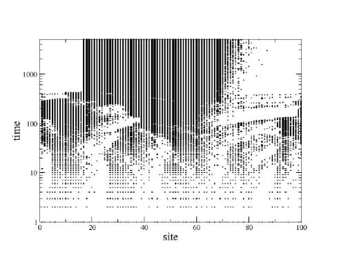
Figure 1: A shock in the TASEP. Space-time diagram for a ring of $N=100$ sites, $\alpha=-50/N$ and density $0.5$. Time evolution of a single clone. The shock is dense and does not advance. Note the logarithmic scale on the $y$-axis.

In Figure 1 we show a space-time diagram of the system with $N=100$ particles, density $0.5$ and $\alpha=-50/N$. The simulation was done with $L=1000$ clones, each of them initialized with random (uniform) occupancy numbers, such that the configuration had density $0.5$. As predicted by the theory [12] for this value of the density, the shock does not drift, although different initial conditions lead to different shock positions. Figure 2 shows the case $\alpha=-30/N$, and density $0.3$: we see that the shock has a net drift to the right, again as predicted by the theory.

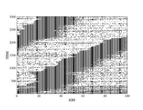
Figure 2: A moving shock in the TASEP. Space-time diagram for a ring of $N=100$ sites, $\alpha=-30/N$ and density $0.3$. The shock drifts to the right.

Let us note here that the configuration corresponds to the end of the time-interval; but one could have sampled one at an intermediate time as explained just below Eq (2.7).

The cloning algorithm has been applied for transport models such as the asymmetric exclusion process and the Kipnis-Marchioro-Presutti model [13, 14, 15] and to study symmetries in fluctuations far from equilibrium [16]. Such studies are useful as a test for the predictions of Fluctuating Hydrodynamics [13, 17], but also to probe the limits of the cloning method itself, when insufficient clone number may yield misleading results (a test criterion has been devised in [14]).

4.3 Continuous-time Markov chains

Many systems have dynamics that are naturally defined in continuous time. For instance, spin flips in the Ising model, that takes the system from a configuration $x$ to another one $y$, can occur at any time with a given rate $W(x\to y)$. To simulate such systems, one can discretize time and the choose a small time step $dt$, (transition probability writing $p(x,y)=dtW(x\to y)$). One then distinguishes between time steps during which a configuration change occurs (with probability, say, $dtW(x\to y)$) and those where nothing happens (with probability $1-dt\sum_{y}W(x\to y)$). Doing this in the algorithm described in the previous sections, one arrives in the limit $dt\rightarrow 0$ at a continuous time version of the cloning algorithm.

One can however also work directly with continuous time simulations. Each configuration $x$ has a total escape rate $r(x)=\sum_{y}W(x\to y)$, which is the rate at which the system jumps from configuration $x$ to any other configuration. One can choose a time interval $\delta t$ from an exponential clock, with probability $p(\delta t)=r(x)\exp[-r(x)\delta t]$, update the time $t\to t+\delta t$, and then decide which configuration changes to make. Going from $x$ to $y$ then occurs with probability $W(x\to y)/\sum_{z}W(x\to z)$. For traditional Monte Carlo algorithms, this method has two advantages. First, one does not have to decide which $dt$ to use and the algorithm makes no discretization error. Second, there are no rejection events which can slow down severely discrete time simulations. However all this comes at the cost of having to generate two random numbers per configuration change (one for the time at which the change occurs, one for the target configuration) while discrete time Monte Carlo only needs one.

When simulating rare events, the continuous time method is more cumbersome to implement but overcomes the problem of diversity of time scales typically met in these simulations. For instance, depending on the value of the bias $\alpha$, the TASEP presented above explores trajectories where the average time between two events ranges from order $1$ (in a traffic jam, only the leading particle can jump forward) to order $1/N$ (when all particles can jump forward). When working with continuous time, the adjustment of the time-step is automatic. In other systems, such as the kinetically constrained models presented in section 5, the situation is even worse. A typical trajectory can explore successive configurations where the waiting times may change by a factor of the order of the system size. In such case, a discrete time algorithm with a time step small enough to resolve the rapid configuration changes will have a prohibitively large number of rejection events when visiting the slow configurations.

To work directly in continuous time, as exposed in [18], the idea is to write the dynamical partition function as a sum over allowed values of $F$ (cfr eq (2.6)):

$$Z_{t}(\alpha)=\langle e^{\alpha F}\rangle=\sum_{x}\underbrace{\sum_{F}e^{\alpha F}P(x,F,t)}_{\equiv\hat{P}(x,\alpha,t)}$$ (4.10)

where $P(x,F,t)$ is the probability density of being in configuration $x$ at time $t$, and having observed a value $F$ of the dynamical observable. The quantity $\hat{P}(x,\alpha,t)$ is its Laplace transform. As in (4.1), we can choose $F$ to be the sum of contributions $f(x\to y)$ occurring at each configuration change. For instance, taking $f(x\to y)=+1$ (resp. $-1$) each time a particle jumps to the right (resp. left) in a 1d particle system corresponds to $F$ being the total particle flux flowing through the system from right to left. We can also consider the case where $F$ depends on the time average of some observable $A(x)$, as in the introduction (see [18, 8]):

$$F=\sum_{k=1}^{K}f\big{(}x_{k-1}\to x_{k}\big{)}+\int_{0}^{t}dt^{\prime}\>A(x(t^{\prime}))$$ (4.11)

where $(x_{0}\ldots x_{K})$ is the sequence of visited configurations of a given history presenting $K$ changes of configurations. $A(x)$ can for instance be the magnetization of the configuration $x$ of a spin system and one is then looking for trajectories that have atypical time average of the magnetization.

From the equation of evolution obeyed by $P(x,F,t)$, one obtains the evolution of $\hat{P}(x,\alpha,t)$:

$$\partial_{t}\hat{P}(x,\alpha,t) = \sum_{y}e^{\alpha f(y\to x)}W(y\to x)\hat{P}(y,\alpha,t)$$

$$-\sum_{y}W(x\to y)\hat{P}(x,\alpha,t)+\alpha A(x)\hat{P}(x,\alpha,t)$$

which is of the form $\partial_{t}|\hat{P}_{\alpha}\rangle=-H_{\alpha}|\hat{P}_{\alpha}\rangle$ where $|\hat{P}_{\alpha}\rangle$ is the vector of components $\hat{P}(x,\alpha,t)$. Just as in Eq (3.2), the modified operator of evolution $H_{\alpha}$ does not conserve probability if $\alpha\neq 0$. We have to proceed as in the steps leading to (4.3) and split the evolution in two contributions, one conserving probability and the other a purely cloning term. To do so we introduce the modified transition rates $W_{\alpha}(y\to x)=e^{\alpha f(y\to x)}W(y\to x)$ and the corresponding escape rate $r_{\alpha}(x)=\sum_{y}W_{\alpha}(x\to y)$. We can then rewrite (4.3) as

$$\partial_{t}\hat{P}(x,\alpha,t) = \overbrace{\sum_{y}W_{\alpha}(y\to x)\hat{P}(y,\alpha,t)-r_{\alpha}(x)\hat{P}(x,\alpha,t)}^{\text{probability conserving}}$$ (4.13)

$$+\underbrace{\big{[}r_{\alpha}(x)-r(x)+\alpha A(x)\big{]}\hat{P}(x,\alpha,t)}_{\text{cloning}}$$

The first part is a modified dynamics of rates $W_{\alpha}(y\to x)$ while the second part corresponds to cloning at rate $r_{\alpha}(x)-r(x)+\alpha A(x)$. The method is then the same as for discrete time dynamics (section 4.1): one takes a large number of copies of the system, each of them evolving in continuous time (i) through the modified rates $W_{\alpha}(y\to x)$ and (ii) subjected to a cloning probability $e^{[r_{\alpha}(x)-r(x)+\alpha A(x)]\Delta t}$ on each time interval $\Delta t$ where the configuration does not change from $x$ [8]. One can rescale the total clone population to keep its size constant, storing as previously the overall cloning factor. The dynamical partition function is then recovered from those factors as in (4.8) and the corresponding dynamical free energy $\mu(\alpha)$ is:

$$\mu(\alpha)=\lim_{t\to\infty}\frac{1}{t}\log Z_{t}(\alpha)$$ (4.14)

We provide in Appendix A an example pseudo-code for the practical implementation of the algorithm.

4.4 An example: density profiles in the ASEP

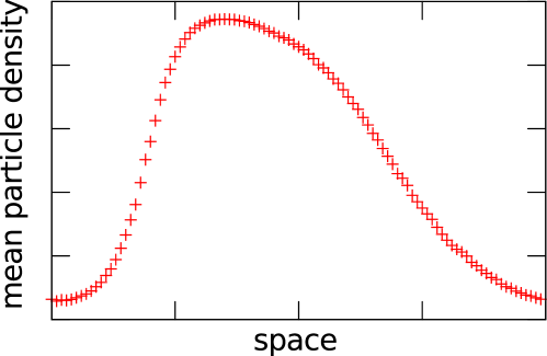
Figure 3: Density profile in the ASEP. $\alpha=-0.3$, $\alpha$ conjugated to the total current flowing through the system. System size is 400, with 200 particles, in periodic boundary conditions, with an asymmetry $E=\frac{1}{2}\log\frac{p}{q}=-0.2.$

Exclusion processes (such as the TASEP studied above) are interesting transport models in which the cloning algorithms can be used and in particular compared to analytical results for the cumulant generating function $\mu(\alpha)=\lim_{t\rightarrow\infty}\ln Z_{t}(\alpha)/t$ [18, 13], including finite size effects [8]. In Fig. 3, we present an example of a mean profile at non-zero $\alpha$ for the asymmetric exclusion process (compared to the TASEP, particles can jump to the left and to the right with respective rates $p$ and $q$). The parameter $\alpha$ is conjugated to the particle flux through the system. We observe on Fig. 3 that, to minimize the overall current, the system develops an asymmetric profile, where only the front particles can jump easily.

5 Fluctuations of Dynamical Activity

Driven systems may reach a non-equilibrium steady state, characterized by a non-zero current the probability distribution of which can be studied as described in the previous section. Another class of non-equilibrium systems is given by glassy systems. In the most simple cases, these systems are out of equilibrium not because they are driven but because their dynamics is so slow that a macroscopic system never reaches Boltzmann equilibrium (or any other steady state), despite the fact that the microscopic dynamics satisfy detailed balance. In this context, it can be interesting to study trajectories of atypical mobility, for instance to detect trajectories that are ‘faster’ or ’slower’ than average, i.e. the dynamic heterogeneity. To quantify this, one introduces the dynamical activity [19, 20, 21] (also termed traffic [22, 23]), which provides a good description of dynamical heterogeneity in glass models, as we now discuss.

On a time window $[0,t]$ the dynamical activity $K$ of a stochastic process is the number of configuration changes undergone by the system, and is thus a random variable that depends on the system’s trajectory.

Kinetically constrained models (KCMs), such as the Fredrickson-Andersen [24] or the Kob-Andersen[25] models are such that static (one-time) properties are trivial in the most simple cases, while their dynamical properties (e.g. two- or more times correlations) share common features with generic glassy phenomena (see [26, 27] for reviews on KCMs). They lend themselves rather easily for the study of their activity $K$, and for the analysis of the results.

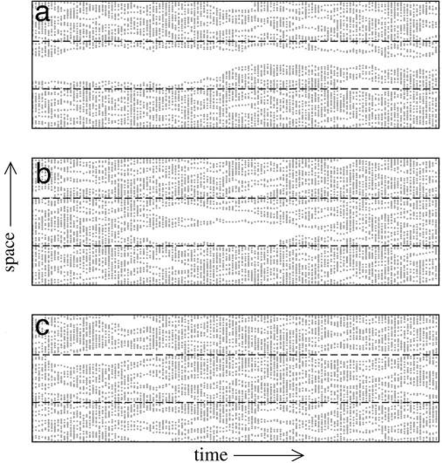
Figure 4: FA model (From Merolle et al. [19]). Space-time diagram of the FA model for atypical (a and b) and typical (c) histories. In the space direction, active sites are represented in black dots while inactive ones are white. The picture is reminiscent of the phase coexistence of a static medium at a solid-liquid coexistence point.

Let us focus for simplicity on the one-dimensional Fredrickson-Andersen (FA) model. It consists in a 1d lattice of $L$ sites. Each site is either excited (low density, active) or unexcited (high density, inactive). The sites may flip from inactive to active (at rate $c$), and from active to inactive (at rate $1-c$). These transitions are allowed on a given site provided at least one of the neighboring sites is active. This is the kinetic constraint, introduced as a way to mimic the facilitated dynamics of molecular glasses, whereby active regions enhance activity in their neighborhood. Clearly, for small values of $c$, the dynamics becomes very slow.

It was observed in [19] that the FA model presents “dynamical coexistence” of active and inactive regions in space-time (see Fig. 4), very similar to the phase coexistence of liquid and solid at the coexistence point in a first order static phase transition –  if one forgets that one direction in Fig. 4 is the time.

The activity $K$ of a configuration is defined as the number of active sites. In practice, one may weight the trajectories followed by the system by a factor $e^{-sK}$, to favor active ($s<0$) or inactive ($s>0$) histories (in this section we take the convention $s=-\alpha$ to follow the notation in the literature on KCMs). If the observed coexistence disappears for $s\neq 0$ (that is, if there is a dynamical phase transition), it means that the system indeed sits on a first-order dynamical coexistence point at $s=0$.

The continuous time cloning algorithm [18] exposed in section 4.3 enables us to compute numerically the dynamical partition function

$$Z_{t}(s)=\langle e^{-sK}\rangle\sim e^{t\mu_{L}(s)}$$ (5.1)

for this system and other KCMs [28, 7] The average is taken on histories of duration $t$, in the large $t$ limit, at fixed system size $L$. The non-analyticities of the dynamical free energy $\mu_{L}(s)$ in the large-size limit, signal the existence of a dynamical phase transition.

Figure 5: FA model (From Garrahan et al. [28]). Numerical evaluation of the “dynamical free energy” $\frac{1}{L}\mu_{L}(s)$ (left) and the density of occupied sites $\rho_{L}(s)$ (right) for histories weighted by $e^{-sK}$. As the system size increases, $\frac{1}{L}\mu_{L}(s)$ approaches its singular limit where $\frac{1}{L}\mu_{L}(s)$ is zero for $s>0$. In the same limit, the density $\rho_{L}(s)$ displays a discontinuity at $s=0$, indicating a first order dynamical transition.

5.1 Dynamical phase coexistence

As shown in [28, 7], several KCMs display a phase transition, in the large system size limit, between an active phase ($s\leq 0$) where the dynamical free energy $\frac{1}{L}\mu_{L}(s)$ is finite, and an inactive phase ($s>0$) where is identically zero (see Fig. 5, left, for the 1d FA model). The mean density of active sites (see Appendix A for details on the practical computation of such a weighted mean)

$$\rho_{L}(s)=\frac{\langle e^{-sK}\frac{1}{t}\int_{0}^{t}\frac{1}{L}\sum_{i=1}^{L}n_{i}\rangle}{\langle e^{-sK}\rangle}$$ (5.2)

(here $n_{i}\in\{0,1\}$ is the activity at site $i$) also characterizes this transition (Fig. 5, right): it remains finite in the active phase $s\leq 0$ (a finite fraction of sites is active) while it goes to zero in the inactive phase (only a finite number of sites remains inactive). Several other glass formers display the same phenomenology (see [29] for a review), representative of dynamical heterogeneities, that is, of the coexistence in the system of regions with high and low dynamical activity.

An interesting question is to determine whether molecular models of glasses, such as Lennard Jones mixtures, also present such a dynamical phase transition. A conceptual difficulty that arises is to find a physically relevant measure of the mobility, that generalizes the concept of dynamical activity to this context. In [30], the activity was defined as the number of events where particles move sufficiently far in a given time-interval, thus averaging out short-scale vibrations, whereas in [31], the activity was taken to be a time-average of the modulus of the forces, in a continuous version of the model. In both approaches, numerical results support the existence of a phase transition at some critical value $s_{c}$. An open issue is to characterize the inactive phase and to determine whether the effective finite-size critical transition parameter $s_{c}(L)$ goes to $0$ as $L$ goes to infinity or not (that is to say: does the standard dynamics at $s=0$ lie exactly at the critical point?).

More generically, the phase transitions are also present in $p$-spin models [32] and in trap models [33], where numerical approach support analytical results. These results are in favor of a generic link between glassiness and dynamical phase coexistence, whose precise nature remains to be understood.

6 Fluctuation of chaoticity in dynamical systems

As explained in the previous section, large deviation theory plays nowadays an important role in non-equilibrium statistical physics to study and quantify dynamical phase transitions. The first studies of large deviations of dynamical observables were however inspired by another field, that of dynamical systems. It was argued in the 70s, following the seminal works of Sinai, Ruelle, Bowen and others [34, 35, 36, 37] that quantitative studies of dynamical systems should rely on a construction analogous to statistical mechanics of trajectory space, where the quantities playing the role of energy functionals for the trajectories are functions of the Lyapunov exponents. This line of thought was very successful in terms of formalism and theory, but progress was severely hampered by the difficulty of computing anything in all but the most schematic systems. Indeed, many of the examples studied very low dimensional systems — mostly maps of the interval, with notable exception of the Lorenz gas [38]. As we show in the two following sections, the development of recent methods to compute the fluctuations of Lyapunov exponents can fill this gap and hopefully lead to new insights in the field of dynamical systems of many bodies.

For sake of concreteness, we will focus on Hamiltonian dynamics but one should keep in mind that the method is much more general and can be applied, for instance, to dissipative systems. We consider a system with $2N$ degrees of freedom whose dynamics is given by

$$\dot{x}_{i}=f_{i}[{\bf x}(t)];\quad\mbox{with}\begin{cases}{\bf x}=(q_{1},\dots,q_{N},p_{1},\dots,p_{N})&\\ {\bf f}=(\frac{\partial H}{\partial p_{1}},\dots,\frac{\partial H}{\partial p_{n}},-\frac{\partial H}{\partial{q_{1}}},\dots,-\frac{\partial H}{\partial{q_{N}}})&\end{cases}$$ (6.1)

As usual to quantify the chaoticity of a trajectory we introduce the Lyapunov exponents. We consider an infinitesimal perturbation ${\bf\delta x}(t)$ whose dynamics reads

$$\delta\dot{\bf x}=-A\cdot\delta{\bf x};\quad\text{with}\quad A_{ij}=-\frac{\partial f_{i}[{\bf x}(t)]}{\partial x_{j}}$$ (6.2)

The evolution of the norm of such a perturbation is given by

$$\frac{{\rm{d}}}{{\rm{d}t}}|\delta{\bf x}|^{2}=-\sum_{ij}2\,\delta x_{i}\,A_{ij}\,\delta x_{j}$$ (6.3)

Introducing the normalized tangent vectors $v_{i}=\frac{\delta x_{i}}{|\delta{\bf x}|}$ whose evolutions are given by

$$\dot{v}_{i}=-\sum_{j}A_{ij}v_{j}+v_{i}\sum_{kl}v_{k}A_{kl}v_{l}$$ (6.4)

equation (6.3) can be recast as

$$\frac{{\rm{d}}}{{\rm{d}t}}|\delta{\bf x}(t)|^{2}=-\sum_{ij}2v_{i}A_{ij}v_{j}|\delta{\bf x}(t)|^{2}$$ (6.5)

and finally solved to yield

$$|\delta{\bf x}(t)|=|{\bf\delta}{\bf x}(0)|{\rm{e}}^{-\sum_{ij}\int_{0}^{t}v_{i}(t^{\prime})A_{ij}[{\bf x}(t^{\prime})]v_{j}(t^{\prime}){\rm{d}t}^{\prime}}$$ (6.6)

The largest Lyapunov exponent is then given by $\lambda=\underset{t\to\infty}{\lim}\lambda(t)$, where the finite time Lyapunov exponent $\lambda(t)$ is

$$\lambda(t)=\frac{1}{t}\log\frac{|\delta{\bf x}(t)|}{|\delta{\bf x}(0)|}=-\frac{1}{t}\int_{0}^{t}{\rm{d}t}^{\prime}\Big{\{}\sum_{ij}v_{i}(t^{\prime})A_{ij}[{\bf x}(t^{\prime})]v_{j}(t^{\prime})\Big{\}}$$ (6.7)

More generally, the exponential expansion of $k$-dimensional volume elements, rather that vectors $\delta{\bf x}$, yields in a similar way the sum of the first $k$ Lyapunov exponents.

To characterize the fluctuations of chaoticity amounts to sampling the distribution of $\lambda(t)$

$$P(\lambda,t)={\rm{e}}^{S(\lambda,t)}\underset{t\to\infty}{\sim}{\rm{e}}^{ts(\lambda)}$$ (6.8)

One can understand that the exponent is generically extensive in time, as in usual thermodynamic systems: one cuts a long trajectory of duration $t$ in many segments of duration $\delta t$ much larger than the typical correlation time $\tau$. Each segment can thus be considered independent of the others and the probability that the total trajectory has an exponent $\lambda$ is

$$P(\lambda,t) = \!\!\!\!\!\!\!\!\!\sum_{(\lambda_{1}+\dots+\lambda_{t/\delta t})\delta t=\lambda t}\!\!\!\!\!\!\!\!\!P_{1}(\lambda_{1},\delta t)\dots P_{t/\delta t}(\lambda_{t/\delta t},\delta t)$$ (6.9)

$$= \!\!\!\!\!\!\!\!\!\sum_{(\lambda_{1}+\dots+\lambda_{t/\delta t})\delta t=\lambda t}\!\!\!\!\!\!\!\!\!{\rm{e}}^{S_{1}(\lambda_{1},\delta t)+\dots+S_{t/\delta t}(\lambda_{t/\delta t},\delta t)}$$ (6.10)

The exponent of each term of the r.h.s. is the sum of $t/\delta t$ terms of order one and is thus of order $t$. At large times, $t/\delta t\gg 1$, the distribution $P(\lambda,t)$ concentrates around its typical value, and the scaling law (6.8) is thus verified. This scaling breaks down in the presence of diverging correlation times, a signature of dynamical phase transitions.

As in statistical mechanics, the derivation of the entropy $s(\lambda)$ is difficult and one rather works in a “canonical” ensemble by introducing a dynamical partition function

$$Z_{t}(\alpha)=\left\langle{\rm{e}}^{\alpha t\lambda(t)}\right\rangle\underset{t\to\infty}{\sim}{\rm{e}}^{t\mu(\alpha)}$$ (6.11)

where the average $\langle\,.\,\rangle$ is made with respect to $P(\lambda,t)$, i.e. over initial conditions, noise realizations, etc. $\mu(\alpha)$ plays the role of $-\beta F$ in statistical mechanics, where $F$ is a free energy, and is called topological pressure.

From the definition of the finite time Lyapunov exponent (6.7), one sees that the computation of $Z_{t}(\alpha)$ amounts to the large deviation computation presented in the introduction, with the observable ${A}$ now given by

$${A}({\bf x})=-\sum_{i,j}v_{i}A_{ij}({\bf x})v_{j};\qquad F=\int dtA({\bf x})$$ (6.12)

Let us now make a point that will be valid for all deterministic systems. In such cases, the only source of fluctuations are the initial conditions. If the system is chaotic enough, this should not be very important but, for example, in the case of mixed system, starting from a regular island or a chaotic region yields a very different result, because trajectories do not take from one to the other. In this review we consider a shortcut to this problem which consists of adding a small amount of stochastic noise, so that the dynamics effectively samples the whole trajectory space (for a discussion of the low noise limit see [40]). We thus consider a slightly different set of equations

$$\dot{q}_{i}=p_{i};\qquad\dot{p}_{i}=-\frac{\partial H}{\partial q_{i}}+\sqrt{2{\epsilon}}\eta_{i}$$ (6.13)

The algorithm presented in the introduction of this paper can now be applied to our noisy Hamiltonian dynamics. We consider a population of ${\cal N}$ clones in phase space of positions and momenta ${\bf q}$ and ${\bf p}$. To each clone we associate a normalized tangent vector ${\bf v}$. We then choose a time step ${\rm{d}t}$ and a noise intensity $\epsilon$ and run the simulation over a large time $t=M{\rm{d}t}$. At $t=0$, the ${\cal N}$ copies of the system start from an arbitrary initial configuration (the noise ensures the ergodicity of the algorithm). At each time step $t^{\prime}=n{\rm{d}t}$, we do the following [39]:

• For each clone

  • $({\bf q},{\bf p})$ evolve with the noisy Hamiltonian dynamics (6.13),

  • ${\bf v}$ evolves according to the linearized dynamics

    $$\dot{v}_{i}=-A_{ij}v_{j}$$ (6.14)

  • ${\bf v}$ is then renormalized to unity and we store the renormalization factor $N(n)=\frac{|{\bf v}(t+dt)|}{|{\bf v}(t)|}\simeq{\rm{e}}^{-{\bf v}^{\dagger}\cdot A\cdot{\bf v}{\rm{d}t}}$.

• Each clone of the system is then pruned or replicated, with its rate $N(n)^{\alpha}$. To do so, we pull a random number $\epsilon$ uniformly between 0 and 1 and we compute $\tau=\lfloor{\epsilon}+N(n)^{\alpha}\rfloor$,

  • if $\tau=0$, the clone is deleted

  • if $\tau>1$, we create $\tau-1$ copies of the clone

• The total population is now composed of ${\cal N}(n+1)$ clones, instead of the initial ${\cal N}(n)$ ones. We then store $R(n)=\frac{{\cal N}(n+1)}{{\cal N}(n)}$,

  • if ${\cal N}(n+1)<{\cal N}(n)$, we copy ${\cal N}(n+1)-{\cal N}(n)$ clones, chosen at random,

  • if ${\cal N}(n+1)>{\cal N}(n)$, we delete ${\cal N}(n+1)-{\cal N}(n)$ clones, chosen at random,

  Finally, we end up again with ${\cal N}(n+1)={\cal N}(n)={\cal N}(0)$ clones.

The dynamical partition function is then obtained from $R(n)$ through

$$Z_{t}(\alpha)=\prod_{n=1}^{M}R(n)$$ (6.15)

while the topological pressure is given by

$$\mu_{t}(\alpha)=\frac{1}{t}\sum_{n=1}^{M}\log R(n)$$ (6.16)

Let us now illustrate this algorithm, called “Lyapunov Weighted Dynamics”, with a low dimensional system (the standard map) and a large dimensional one (a FPU chain of 1024 particles).

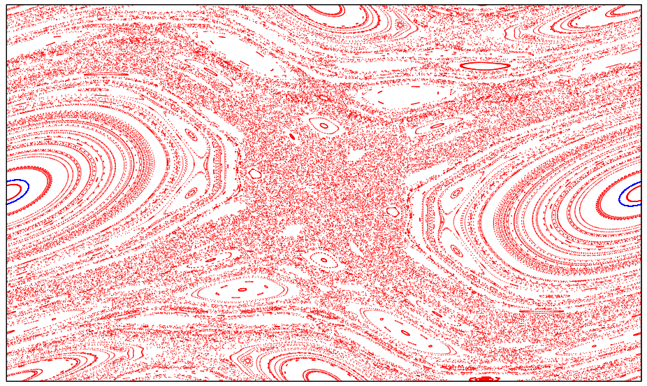
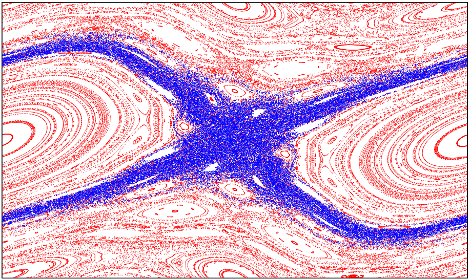
$\alpha=-0,04$

$\alpha=0,04$

Figure 6: Typical Configurations for $\alpha=\pm 0,04$. Phase space trajectories of the standard map are shown in light red whereas the trajectories localized by the Lyapunov Weighted Dynamics appear in dark blue.

6.1 The Standard Map

The standard map is defined by the dynamics

$$p_{n+1}=p_{n}+\frac{k\delta}{2\pi}\sin(2\pi q_{n});\qquad q_{n+1}=q_{n}+\delta p_{n+1}$$ (6.17)

with $(q_{n},p_{n})\in[0,1]\times[-1,1]$. It is one of the traditional models used to study transition to chaos. It goes from an integrable system when $k=0$ to a more and more chaotic one when $k$ increases. In figure 6 we show the typical trajectories that are localized by the Lyapunov Weighted Dynamics for very small bias ($\alpha=\pm 0.04$). One sees that as soon as the system is biased in favor of integrable trajectories ($\alpha<0$), the dynamics localizes on integrable islands, whereas a tiny bias favoring chaotic trajectories ($\alpha>0$) detects the chaotic layers surrounding these islands.

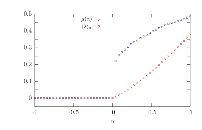
Figure 7: Standard map. Dynamical free energy $\mu(\alpha)$ (red crosses) and average Lyapunov exponent $\langle\lambda\rangle_{\alpha}=Z_{t}^{-1}(\alpha)\langle\lambda{\rm{e}}^{\alpha\lambda t}\rangle$ (blue squares) as a function of the bias $\alpha$. The discontinuity at $\alpha=0$ of $\langle\lambda\rangle_{\alpha}=\mu^{\prime}(\alpha)$ is the signature of a phase coexistence between chaotic and integrable trajectories in space time.

Computing the topological pressure (figure 7) shows that the system lies at a critical point where chaotic and integrable trajectories coexist in phase space, in the manner of a first order phase transition.

6.2 FPU chains

Beyond the computation of dynamical free energies (or topological pressure), the algorithm can be used to sample trajectories of atypical chaoticity. Let us show here on a high-dimensional system, with 2048 degrees of freedom, which are the trajectories that realize large deviations of the chaoticity in anharmonic chains of oscillators. We consider the following Hamiltonian

$${\cal H}=\sum_{i=1}^{N}\frac{p_{i}^{2}}{2}+\sum_{i=1}^{N}\left[\frac{(x_{i+1}-x_{i})^{2}}{2}+\beta\frac{(x_{i+1}-x_{i})^{4}}{4}\right]$$ (6.18)

where $x_{N+1}=x_{1}$. This system, studied in the 50s by Fermi, Pasta, Tsingou and Ulam, corresponds to $N$ particles connected by anharmonic springs. The limit $\beta=0$ corresponds to an integrable case: the springs are harmonic and the Fourier modes correspond to $N$ independent harmonic oscillators or frequencies

$$\omega_{k}=2\sin\left(\frac{\pi k}{N}\right)$$ (6.19)

There has been continuous interest in this model (for a review see [41]) because of its rich phenomenology, and in particular, there has been some recent studies of the (Gaussian) fluctuations of its Lyapunov exponent [42]. As soon as $\beta$ is non-zero, the dynamics are chaotic. However, starting from well chosen initial conditions, the model admits long-lived solitonic modes, related to the Korteweg-de Vries modified equation [43]. Similarly, a modulational instability leads to short-lived chaotic breathers [44, 45], when energy is injected in high-frequency modes. If one runs an equilibrium simulation of the anharmonic chain, one typically observes a mixture of short-lived localized structures (solitons, breathers) and a phonon bath (figure 8).

When applying the Lyapunov Weighted Dynamics, we add a small stochastic noise to the system, taking care that the noise conserves the total energy and momentum and thus preventing a slow, unphysical drift in these quantities.

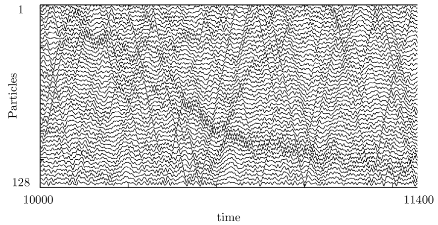
Figure 8: Equilibrium simulations of the FPU chain ($N=128,\,\alpha=0$). Time-line of each of the 128 particles around their [arbitrary] equilibrium positions. We see a superposition of localized breathers, ballistic solitons and small fluctuations.

If one biases the system in favor of regular trajectories, the phonons and breathers completely disappear and we observe a long-lived gas of solitons, propagating ballistically (see figure 9). In this case, it is important to set the center of mass velocity to zero, because otherwise the system can eliminate completely chaoticity by concentrating all its energy on the center of mass motion.

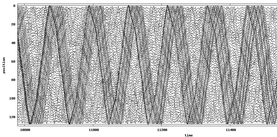
Figure 9: Looking for regular trajectories ($N=128,\,\alpha=5\,N$). Simulation at fixed energy ($E=1$) with fixed boundary conditions, starting from microcanonical equilibrium. The figure shows the time-line of each particles around its [arbitrary] equilibrium position. Several solitons are ballistically propagating from one end of the system to the other, where it elastically bounce of fixed boundary condition. the Lyapunov exponent of this trajectory is equal to half the average one.

On the other extreme, a bias in favor of chaotic trajectories localizes long-lived chaotic breathers (see figure 10). We used periodic boundary conditions for this simulation to reduce the interactions between the wandering breather and the boundaries of the system. Note that running the same simulation in a much larger system (N=1024) shows that the breathers are much more localized than the solitons (figure 11).

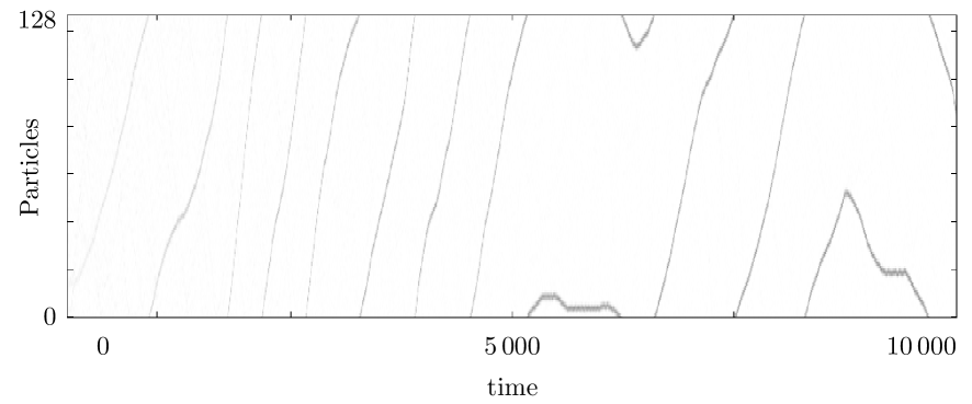
Figure 10: Looking for chaotic trajectories ($N=128,\,\alpha=5\,N$) This simulation is realized at fixed energy and total momentum (energy density $E=1$) with periodic boundary conditions. The gray level represent the total energy of each particles. Starting from an equilibrium configuration, the dynamics reveals a chaotic breathers whose Lyapunov exponent is three time larger than the average one.

Interestingly, the values of the bias $\alpha$ we have to use here are not of order one. Indeed, as $N$ increases, the distribution of the largest Lyapunov exponent becomes more and more peaked. Let us assume for instance that $s(\lambda)$ is extensive with some power of the system size, so that one can write

$$P(\lambda_{1},t)=\exp[N^{\xi}t\tilde{s}(\lambda_{1})]$$ (6.20)

with $\tilde{s}(\lambda)$ of order 1 in both $t$ and $N$. From the expression

$$Z_{t}(\alpha)=\left\langle{\rm{e}}^{\alpha\lambda t}\right\rangle=\int d\lambda\exp[N^{\xi}t\tilde{s}(\lambda_{1})+\alpha\lambda t]$$ (6.21)

one sees that the integral is dominated by a value $\lambda^{*}$ such that:

$$\tilde{s}^{\prime}(\lambda^{*})=-\frac{\alpha}{N^{\xi}}$$ (6.22)

When $N\to\infty$, $\lambda^{*}$ satisfies $s^{\prime}(\lambda^{*})=0$ and is thus the typical value of the Lyapunov exponent. One should thus use a bias that scales as $\alpha=N^{\xi}\tilde{\alpha}$ to observe large deviations of the Lyapunov exponents. Similarly, to access the dynamical free energy, one has to compute the exponent $\xi$ and define

$$\tilde{\mu}(\tilde{\alpha})=\frac{1}{tN^{\xi}}\log Z_{t}(\alpha)$$ (6.23)

Such a calculation, which, as far as we know, has not been done so far, would tell if the FPU chain lies at a critical point where breathers, solitons and phonons coexist in a first order phase transition manner. The computation of the dynamical free energy for large dimensional systems is now achievable numerically and is one of the exciting goal that are facing us.

Figure 11: Looking for chaotic trajectories ($N=1024,\,\alpha=5\,N$) . This simulation is realized at fixed energy and total momentum (energy density $E=1$) with periodic boundary conditions. The gray level represent the total energy of each particles.

7 Work and entropy production

When a system is subjected to an external drive, the total energy absorbed (and the resulting entropy production), are quantities that fluctuate depending on the initial microscopic configuration of the system and on the thermal bath, if there is one. Work and entropy production are important quantities, because they concern the state of the system and are the subject of the Second Law of thermodynamics. The Second Law as such concerns only average quantities, and not the fluctuations. It was only relatively recently realized that a wider framework – based on considering the effect of time-reversal on the dynamics – allows to derive a set of relations that are obeyed by the fluctuations – well beyond the linear regime – and yields the Second Law constraints as particular cases.

i) The transient Fluctuation Theorem relates, in the same context, the probability of a given work $W$, and that of its opposite: $P(W)/P(-W)=e^{W/T}$ [46, 47].

ii) The Jarzynski relation states that the average of $e^{-W/T}$ over all processes starting from an equilibrium distribution at temperature $T$ is one [48].

Both are very general, model-independent results, and were later shown to be particular cases of the more general relation, Crooks’ relation.

iii) The stationary fluctuation theorem involves the same relation for the work as the transient version, in a stationary (non-equilibrium) situation, and is valid only in the limit of large times. The particular case in which the dynamics is deterministic (the Gallavotti-Cohen theorem [47]) deserves special attention: the theorem is non trivial because the nature of the stationary distribution is then dependent upon the ergodicity properties of the system. These conditions involve not only chaoticity properties of the attractor, as one would expect from any problem in ergodic theory, but also the fact that attractor and repellor sets are sufficiently intertwined: large deviation trajectories that commute between them generate the reversals in entropy production [49].

Systems with macroscopic, hydrodynamic degrees of freedom may have extremely large fluctuations when subjected to strong forcing, due to excitation of macroscopic structures [50]. The typical example is the (Rayleigh-Bénard) convection of a fluid between a hot $T_{h}$ lower plate and a colder $T_{c}$ top plate [51]. The heat is transported by fluid currents that have macroscopic fluctuations, enormous compared with $k_{b}T_{h}$. The fluctuation theorem as such involves the temperatures $T_{h},T_{c}$ that are irrelevant for these fluctuations. The only way in which the appearance of a Fluctuation Relation for the hydrodynamic modes may be justified, is to invoke the existence of a large effective temperature, related to the macroscopic fluctuations. Bonetto and Gallavotti [52] have conjectured that this could be justified by considering the restricted space in which the macroscopic takes place. These questions are very much open, and in order to make progress it would be useful to simulate the limits beyond which the fluctuation theorem ceases to hold rigorously, because that is where new concepts may arise. These are the limits in which large deviations are particularly hard to observe, if one has to wait for them to happen spontaneously.

7.1 Sinai billiard

The method of cloning has been shown to work efficiently in the verification of the Gallavotti-Cohen theorem on a simple chaotic system given by the Sinai billiard. This system consists of a particle moving inside a billiard as in figure 12, with periodic boundary conditions. It is under the action of a force field $\vec{E}$, and is subject to a deterministic thermostat that keeps the velocity modulus constant $|\vec{v}|=1$. Between bounces, the equations of motion are:

$$\ddot{x}_{i} = -E_{i}+\gamma(t)\dot{x}_{i},\qquad i=1,2;$$

$$\gamma(t) = \sum_{i}E_{i}\dot{x}_{i}.$$ (7.1)

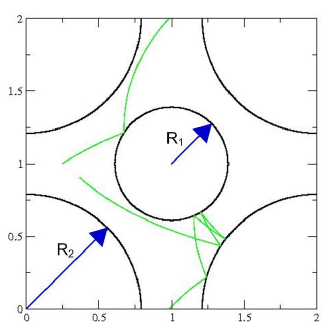
Figure 12: The Sinai billiard. The radii are $R_{1}=0.39,R_{2}=0.79$. We also show an example of trajectory for the external field $\vec{E}=(1,0)$.

We wish to calculate the fluctuations of the dissipated power $\gamma$ and thus the dynamical partition function

$$Z_{t}(\alpha)=\langle{\rm e}^{\alpha\int_{0}^{t}\gamma(t^{\prime})dt^{\prime}}\rangle$$ (7.2)

The fluctuation theorem arises from the symmetry

$$\mu(\alpha)=\mu(-1-\alpha)$$

with $\mu(\alpha)=\lim_{t\to\infty}\frac{1}{t}\ln Z_{t}(\alpha)$. Therefore with reference to the notation of the first section we have now

$$A(x)=\gamma(x)$$

As in the previous section, the dynamics is deterministic, and hence to allow different clones to diversify, we introduce a small stochastic noise, (cfr paragraph leading to equation (6.13)) and check the stability of results in the limit of small noise. We evolve the system for macroscopic intervals ${\cal{T}}$, and clone at time $t^{\prime}=n{\cal T}$ with a factor

$$k_{t^{\prime}}=e^{\alpha\int_{t^{\prime}}^{t^{\prime}+{\cal{T}}}\gamma(t^{\prime\prime})\,dt^{\prime\prime}}\;.$$

Before each deterministic step of time ${\cal{T}}$, clones are given random kicks of variance $\Delta$ in position and/or velocity direction. The time-interval ${\cal{T}}$ and the noise intensity $\Delta$ are chosen so that twin clones have a chance to separate during time ${\cal{T}}$, and this depends on the chaotic properties of the system. In the present case, $0.1\leq{\cal{T}}\leq 1$ allows for a few collisions, which guarantees clone diversity for $10^{-3}\leq\Delta\leq 10^{-4}$.

In Fig. 13 we show the results of $\mu(\alpha)$ for $-2\leq\alpha\leq 1$, and for $\vec{E}=(E,0)$ with $E=1$ and $E=2$, both corresponding to very large current deviations (in the figure $\alpha$ is called $\lambda$).

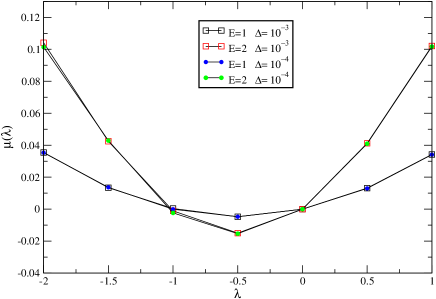
Figure 13: The Gallavotti-Cohen theorem. Plot of $\mu(\lambda)$ vs. $\lambda$ for the driven Lorentz gas. Data for $\vec{E}=(E,0)$, $E=1,2$ and noise intensity $\Delta=10^{-3},10^{-4}$. The Gallavotti-Cohen theorem implies the symmetry around $\lambda=-1/2$. The continuous lines represents a polynomial fit, quadratic for $E=1$ (Gaussian behavior), 4-th order for $E=2$.

8 Planetary systems

Planetary systems are the epitome of deterministic systems. With their relatively small number of interacting bodies, they could easily be considered the systems that are further from statistical treatment. And yet, statistical analysis of orbits becomes necessary: when we discover a planetary system we find that many amongst the observationally allowed configurations are only stable in the immediate past or future [53]. Since we do not expect that just by chance we came across a system that has just ejected (or will soon eject) a planet, we tend to favor amongst configurations compatible within error with the data, those that have an unusually high level of stability.

On a related line, it has been shown [54] that just considering a shift in the Earth’s present position of the order of one hundred meters, the fate of Mercury may change dramatically, in some cases leading its orbit to intersect the one of Venus. Consider for example the study by Laskar [54]. In a first calculation, he integrated the orbit of Mercury starting from different configurations, obtained by displacing the position of the earth by about $150$ meters. The orbits obtained this way were qualitatively similar, and yet different. Next, he repeated the calculation but making a few clones of the trajectories, and choosing the one with largest eccentricity. After a few such steps, he reached orbits with great eccentricities, that could cross the orbit of Venus. We recognize here a strategy that is very close to the one we are describing here, for the particular cases $\alpha=0$ and $\alpha=\infty$, respectively. The small displacements are in fact playing the role of our noise.

Indeed, if at each cloning step we had cloned or killed configurations in a fraction proportional to $\alpha$ times the eccentricity change during the corresponding time interval (cfr. Section 3: the eccentricity plays here the role of $\phi$ described there) we would have obtained the full probability distribution of, say, the eccentricity at each time. Denote $N(\alpha)$ the total number of clones at time $t$ obtained without normalizing the clone population, or keeping track of the normalizations if they were done. $N(\alpha)$ is the Laplace transform of the probability $P(e)$:

$$N(\alpha)=\int de\;e^{-\alpha e}\;P(e)$$ (8.1)

Just as in the example of Sinai’s billiard, because the system is chaotic, the displacements (or the noise level), may be essentially negligible – for example, compatible with all other external sources of displacements which we have neglected — and yet yield all the variety of trajectories.

It would be very interesting to see these methods applied to studying in detail the possible future and past evolution of planetary systems, with a large deviation statistical analysis. Many interesting questions concerning the self-organization of the stability of our solar system could be investigated this way.

Appendix A Cloning in continuous time: an example pseudo-code

In this appendix we provide an example pseudo-code for the cloning of a system described by a configuration conf, evolving with Markov dynamics in continuous time (see section 4.3). The dynamics of each clone consists in a succession of (i) Poissonian waiting times (sampled with the function random.poisson) between jumps (ii) change of configuration, or “jumps” (performed by evolve()) and (iii) cloning, keeping the total number of clone constant. The way in which the weighted average of a time-extensive observable obs is computed is also explicited: a value of obs is attached to each clone and copied/pruned with it.

alpha=0.1          # parameter conjugated to the observable F
N=500              # number of clones
time=0             # initial time
tmax=1000          # maximum simulation time
cloning=0          # logarithm of the global cloning factor
                   # at the end the ldf is given by cloning/time
conf.init()        # initialization of the clones:
                   #   conf[1] to conf[N] are set to given configurations
escaperate.init()  # initialization of the alpha-dependent escape rates
obs.init()         # initialize an observable obs that we want to average
                   # over weighted histories

# initialisation of first jump times
for c from 1 to N do:
  jumptime[c]=random.poisson(escaperate[c])   # Poisson law of rate escaperate[c]

# main loop

while t<tmax do
  (c,t)=next(jumptime)    # returns the first clone c to jump, and its jumptime t
  conf[c].evolve()        # evolves the configurations clone c
                          # note that the observable obs is evolved accordingly
  deltaT=random.poisson(escaperate[c])
                          # determines the time interval until the next jump
  jumptime[c]+=deltaT     # updates the jumptime
  K=conf[c].clfact(deltaT)# yields the cloning factor
                          #  K=e^(deltaT*(deltaescaperate[c]+alpha*A[c]))
  cloning+=log((N+K-1)/N) # updates the log of the global cloning factor

  k=floor(K+random.real())# integer number k representing the number of clones
                          # replacing the current clone c

  cases
    k=0: # clone c is suppressed, i.e. replaced by another one chosen at random
      do newc=random.integer(N) while newc==c
      conf[c]=conf[newc]
      obs[c]=obs[newc]
      jumptime[c]=jumptime[newc]
    k=1: # nothing is done
    k>1: # k-1 copies of c have to be done; then, among the total N+k-1
         # resulting clones, k-1 of them are pruned so as to keep N constant
      indices=randomarray(N,k)
         # puts in indices  k-1 *different* random integers between 1 and Nclones+k-1
         # (both included); only those less or equal than N will be replaced by c
      for newc in indices do:
         if newc<=N do:
            conf[newc]=conf[c]
            obs[newc]=obs[c]
            jumptime[newc]=jumptime[c]

# output of results
ldf=cloning/time
print(’large deviation function = ’,ldf)
meanobs=sum(obs[c] for c in range(N))/N/time
print(’weighted mean of observable = ’,meanobs)

References

- [1] H. Touchette, Physics Reports 478 (2009) 1
- [2] J. B. Anderson, J. Chem. Phys 63 1499 (1975)
- [3] D. Aldous and U. Vazirani, in Proc. 35th IEEE Sympos. on Foundations of Computer Science (1994)
- [4] P. Grassberger, Comp. Phys. Comm. 147 64-70 (2002 )
- [5] P. Del Moral P, A. Doucet, A. Jasra, Jou. Royal Stat. Soc. B - Stat. Meth. 68 411-436 (206)
- [6] C. Giardina, J. Kurchan and L. Peliti, Phys. Rev. Lett. 96 (2006) 120603.
- [7] J.-P. Garrahan, R.L. Jack, V. Lecomte, E. Pitard, K. van Duijvendijk, and F. van Wijland, J. Phys A: Math. Theor. 42 (2009) 075007
- [8] J. Tailleur and V. Lecomte AIP Conf. Proc 1091 (2009) 212, Modeling and Simulation of New Materials
- [9] U. Frisch, Turbulence. The legacy of A. N. Kolmogorov. Cambridge University Press, Cambridge (UK), 1995.
- [10] M. El Makrini, B. Jourdain, T. Lelièvre, Diffusion Monte Carlo method: Numerical analysis in a simple case, ESAIM, Math. Model. Numer. Anal. 41 (2007) 189.
- [11] W. Cochran, Sampling techniques, Wiley India Pvt. Ltd., 2007.
- [12] T. Bodineau, B. Derrida, Phys. Rev. E 72 (2005) 066110
- [13] P. I. Hurtado and P. L. Garrido, Phys. Rev. Lett. 102 (2009) 250601
- [14] P. I. Hurtado and P. L. Garrido, J. Stat. Mech. P02032 (2009)
- [15] P. I. Hurtado and P. L. Garrido, Phys. Rev. E 81 (2010) 041102
- [16] P. I. Hurtado, C. Pérez-Espigares, J. J. del Pozo and P. L. Garrido, Proc. Natl. Acad. Sci. USA 108, 7704
- [17] P. I. Hurtado, P. L. Garrido, arxiv:1106.0690
- [18] V. Lecomte and J. Tailleur, J. Stat. Mech. P03004 (2007)
- [19] M. Merolle, J.-P. Garrahan, and D. Chandler, Proc. Natl. Acad. Sci. U.S.A. 102 (2005) 10837
- [20] V. Lecomte, C. Appert-Rolland, and F. van Wijland, Comptes Rendus Physique 8 (2007) 609
- [21] T. Bodineau and R. Lefevere J. Stat. Phys. 133 (2008) 1
- [22] C. Maes, K. Netocný, and B. Wynants, Markov Processes Relat. Fields 14 (2008) 445
- [23] C. Maes and K. Netocný, Europhys. Lett. 82 (2008) 30003
- [24] G.H. Fredrickson and H.C Andersen H C Phys. Rev. Lett. 53 (1984) 1244
- [25] W. Kob and H. C. Andersen Phys. Rev. E 48 (1993) 4364
- [26] F. Ritort and P. Sollich, Adv. Phys. 52 (2003) 219
- [27] J.-P. Garrahan, P. Sollich, C. Toninelli in Dynamical heterogeneities in glasses, colloids and granular materials (Oxford University Press 2011)
- [28] J.-P. Garrahan, R.L. Jack, V. Lecomte, E. Pitard, K. van Duijvendijk, and F. van Wijland, Phys. Rev. Lett. 98 (2007) 195702
- [29] D. Chandler and J.-P. Garrahan, Annual Review of Physical Chemistry 61 (2010) 191
- [30] L.O. Hedges, R.L. Jack, J.-P. Garrahan, and D. Chandler, Science 323 (2009) 1309
- [31] E. Pitard, V. Lecomte, and F. Van Wijland, arXiv:1105.2460 (2011)
- [32] K. van Duijvendijk, R. L. Jack, and F. van Wijland, Phys. Rev. E 81 (2010) 011110
- [33] K. van Duijvendijk, G. Schehr, and F. van Wijland, Phys. Rev. E 78 (2008) 011120
- [34] Y. G. Sinai, Russ. Math. Surveys 27, 21 (1972)
- [35] R. Bowen. Equilibrium States and the Ergodic Theory of Anosov Diffeomorphism, volume 470 of Lecture Notes in Math. Springer, Berlin, (1975).
- [36] D. Ruelle. Inventiones Mathematicae, 34, 231, (1976).
- [37] D. Ruelle. Thermodynamic Formalism. Addison-Wesley, (1978).
- [38] H. van Beijeren and O. Mülken. Phys. Rev. E, 71, 036213, (2005).
- [39] J. Tailleur, J. Kurchan,Nat. Phys., 3, p. 203-207, (2007)
- [40] J. Kurchan, J. Stat. Phys. 128, 1307 (2007).
- [41] G.P. Berman and F.M. Izrailev. Chaos, 15, 015104, (2005).
- [42] Pavel V. Kuptsov, Antonio Politi, arxiv:1102.3141 (2011)
- [43] M.D. Kruskal and N.J. Zabusky. J. Math. Phys., 5, 231, (1964).
- [44] T. Cretegny, T. Dauxois, S. Ruffo, and A. Torcini. Physica D, 121, 109–126, (1998).
- [45] A. Trombettoni and A. Smerzi. Phys. Rev. Lett., 86, 2353–2356, (2001).
- [46] Evans D J, Cohen E G D, and Morriss G P, Phys. Rev. Lett. 71 2401 (1993)
- [47] Gallavotti G and Cohen E G D, Phys. Rev. Lett. 74 2694 (1995)
- [48] Jarzynski C, Phys. Rev. Lett. 78 2690 (1997)
- [49] Kurchan J. (2007), J. Stat. Phys. 128, 1307.
- [50] Portelli B, Holdsworth PCW, Pinton JF, Phys. Rev. Lett. 90 104501 (2003)
- [51] Ciliberto S, Laroche C, J. Phys. (Paris) 8 :215-219 (1998)
- [52] F. Bonetto and G. Gallavotti Comm. Math. Phys. 189 263 (1997)
- [53] Barnes, R; Quinn, T, Astrophysical Journal 611 494 (2004)
- [54] J. Laskar, Astron. Astrophys. 287, L9 (1994)