Belief-propagation algorithm and the Ising model on networks with arbitrary distributions of motifs

Abstract

We generalize the belief-propagation algorithm to sparse random networks with arbitrary distributions of motifs (triangles, loops, etc.). Each vertex in these networks belongs to a given set of motifs (generalization of the configuration model). These networks can be treated as sparse uncorrelated hypergraphs in which hyperedges represent motifs. Here a hypergraph is a generalization of a graph, where a hyperedge can connect any number of vertices. These uncorrelated hypergraphs are tree-like (hypertrees), which crucially simplifies the problem and allows us to apply the belief-propagation algorithm to these loopy networks with arbitrary motifs. As natural examples, we consider motifs in the form of finite loops and cliques. We apply the belief-propagation algorithm to the ferromagnetic Ising model with pairwise interactions on the resulting random networks and obtain an exact solution of this model. We find an exact critical temperature of the ferromagnetic phase transition and demonstrate that with increasing the clustering coefficient and the loop size, the critical temperature increases compared to ordinary tree-like complex networks. However, weak clustering does not change the critical behavior qualitatively. Our solution also gives the birth point of the giant connected component in these loopy networks.

I Introduction

The belief-propagation algorithm is an effective numerical method for solving inference problems on sparse graphs. It was originally proposed by J. Pearl Pearl:p88 for tree-like graphs. The belief-propagation algorithm was applied to study diverse systems in computer science, physics, and biology. Among its numerous applications are computer vision problems, decoding of high performance turbo codes and many others, see Frey:98 ; McEliece:mmc98 . Empirically, it was found that this algorithm works surprisingly good even for graphs with loops. J. S. Yedidia et al. Yedidia:yfw01 found that the belief-propagation algorithm actually coincides with the minimization of the Bethe free energy. This discovery renewed interest in the Bethe-Peierls approximation and related methods Pretti:pp03 ; Mooij:mk05 ; Hartmann:hw05 . In statistical physics the belief-propagation algorithm is equivalent to the so-called cavity method proposed by Mézard, Parisi, and Virasoro mp2003 . The belief-propagation algorithm is applicable to models with both discrete and continuous variables mooij04 ; ohkubo05 ; Dorogovtsev:dgm08 . Recently the belief-propagation algorithm was applied to diverse problems in random networks: spread of disease karrer10 , the calculation of the size of the giant component sk10 , counting large loops in directed random uncorrelated networks bianconi08 , the graph bi-partitioning problem sulc10 , analysis of the contributions of individual nodes and groups of nodes to the network structure ras10 , and networks of spiking neurons smd09 .

These investigations showed that the belief-propagation algorithm is exact for a model on a graph with locally tree-like structure in the infinite size limit. However, only an approximate solution was obtained by use of this method for networks with short loops. Real technological, social and biological networks have numerous short and large loops and other complex subgraphs or motifs which lead to essentially non-tree-like neighborhoods ab01a ; dm01c ; Dorogovtsev:2010 ; Newman:n03a ; Milo2002 ; Milo2004 ; Sporn2004 ; Alon2007 . That is why it is important to develop a method which takes into account finite loops and more complex motifs. Different ways were proposed recently to compute loop corrections to the Bethe approximation by use of the belief-propagation algorithm mr05 ; ps05 . These methods, however, are exact only if a graph contains a single loop. Loop expansions were proposed in Refs. Chertkov:cc06a ; Chertkov:cc06b . However, they were not applied to complex network yet.

Recently, Newman and Miller newman:n09 ; m09 ; kn10b independently introduced a model of random graphs with arbitrary distributions of subgraphs or motifs. In this natural generalization of the configuration model, each vertex belongs to a given set of motifs [e.g., vertex $i$ is a member of $Q^{(1)}(i)$ motifs of type $1$, $Q^{(2)}(i)$ motifs of type $2$, and so on], and apart from this constraint, the network is uniformly random. In the original configuration model, the sequence of vertex degrees $Q(i)$ is fixed, where $i=1,2,...,N$. In this generalization, the sequence of generalized vertex degrees $Q^{(1)}(i),Q^{(2)}(i),...$ is given. For example, motifs can be triangles, loops, chains, cliques (fully connected subgraphs), single edges that do not enter other motifs, and, in general, arbitrary finite clusters. The resulting networks can be treated as uncorrelated hypergraphs in which hyperedges represent motifs. In graph theory, a hypergraph is a generalization of a graph, where a hyperedge can connect any number of vertices Berge73 . Because of the complex motifs, the large sparse networks under consideration can have loops, clustering, and correlations, but the underlying hypergraphs are locally tree-like (hypertrees) and uncorrelated similarly to the original sparse configuration model. Our approach is based on the hypertree-like structure of these highly structured sparse networks. To demonstrate our approach, we apply the generalized belief-propagation algorithm to the ferromagnetic Ising model on the sparse networks in which motifs are finite loops or cliques. We obtain an exact solution of the ferromagnetic Ising model and the birth point of the giant connected component in this kind of highly structured networks. Note that the Ising model on these networks is a more complex problem than the percolation problem because we must account for spin interactions between spins both inside and between motifs. We find an exact critical temperature of the ferromagnetic phase transition and demonstrate that finite loops increase the critical temperature in comparison to ordinary tree-like networks.

II Ensemble of random networks with motifs

Let us introduce a statistical ensemble of random networks with a given distribution of motifs in which each vertex belongs to a given set of motifs and apart of this constraint, the networks are uniformly random. These networks can be treated as uncorrelated hypergraphs, in which motifs play a role of hyperedges, so the number of hyperdegrees are equal to the number of specific motifs attached to a vertex. In principal, one can choose any subgraph with an arbitrary number of vertices as a motif, see Fig. 1. In the present paper, for simplicity, we only consider simple motifs such as single edges, finite loops, and cliques.

Let us first note how one can describe a statistical ensemble of random networks with the simplest motifs, namely simple edges (see, for example, Refs. Dorogovtsev:dgm08 ; Bianconi09 and references therein). We define the probability $p_{2}(a_{ij})$ that an edge between vertices $i$ and $j$ is present ($a_{ij}=1$) or absent ($a_{ij}=0$),

$$p_{2}(a_{ij})=\frac{\left\langle Q_{2}\right\rangle}{N-1}\delta(a_{ij}-1)+\Bigl{(}1-\frac{\left\langle Q_{2}\right\rangle}{N-1}\Bigr{)}\delta(a_{ij})$$ (1)

where $a_{ij}$ are entries of the symmetrical adjacency matrix, $\langle Q_{2}\rangle=\langle Q\rangle$ is the mean number of edges attached to a vertex. It is well known that the probability of the realization of the Erdős-Rényi graph with a given adjacency matrix $a_{ij}$, is the product

$$G_{2}(\{a_{ij}\})=\prod_{i=1}^{N-1}\prod_{j=i+1}^{N}p_{2}(a_{ij}).$$ (2)

The degree distribution is the Poisson distribution. In the configuration model, the probability of the realization of a given graph with a given sequence of degrees, $Q_{2}(1)$, $Q_{2}(2)$, $Q_{2}(3)$,…, $Q_{2}(N)\equiv\{Q_{2}(i)\}$, is

$$G_{2}(\{a_{ij}\})=\frac{1}{A}\prod_{i=1}^{N}\delta\Bigl{(}Q_{2}(i)-\sum_{j=1}^{N}a_{ij}\Bigr{)}\prod_{i<j}p_{2}(a_{ij}).$$ (3)

The delta-function fixes the number of edges attached to vertex $i$. $A$ is a normalization constant. The distribution function of degrees is determined by the sequence $\{Q_{2}(i)\}$,

$$P_{2}(Q_{2})=\frac{1}{N}\sum_{i}\delta(Q_{2}-Q_{2}(i)).$$ (4)

The second simplest motif, the triangle, plays the role of a hyperedge that interconnects a triple of vertices. Let us introduce the probability $p_{3}(a_{ijk})$ that a hyperedge (triangle) among vertices $i$, $j$, and $k$ is present or absent, i.e., $a_{ijk}=1$ or $a_{ijk}=0$, respectively:

$$p_{3}(a_{ijk})=p\delta(a_{ijk}-1)+(1-p)\delta(a_{ijk}),$$ (5)

where

$$p=\frac{2\left\langle Q_{3}\right\rangle}{(N-1)(N-2)}$$ (6)

is the probability that vertices $i,j$ and $k$ form a triangle. $\left\langle Q_{3}\right\rangle$ is the mean number of triangles attached to a randomly chosen vertex. $a_{ijk}$ are entries of the adjacency matrix of the hypergraph. This matrix is symmetrical with respect to permutations of the indices $i,j$ and $k$, $a_{ijk}=a_{jki}=a_{kij}=\dots$  .

For example, one can introduce the ensemble of the Erdős-Rényi hypergraphs. Given that the matrix elements $a_{ijk}$ are independent and uncorrelated random parameters, the probability of realization of a graph with a given adjacency matrix $a_{ijk}$ is the product of probabilities $p_{3}(a_{ijk})$ over different triples of vertices:

$$G_{3}(\{a_{ijk}\})=\prod_{i=1}^{N-2}\prod_{j=i+1}^{N-1}\prod_{k=j+1}^{N}p_{3}(a_{ijk}).$$ (7)

This function describes the ensemble of the Erdős-Rényi hypergraphs with the Poisson degree distributions of the number of triangles attached to vertices,

$$P_{3}(Q_{3})=\frac{(\langle Q_{3}\rangle)^{Q_{3}}}{Q_{3}!}e^{-\langle Q_{3}\rangle}.$$ (8)

In the configuration model, the probability of the realization of a given graph with a sequence of the number of triangles, $Q_{3}(1)$, $Q_{3}(2)$, $Q_{3}(3)$,…,$Q_{3}(N)\equiv\{Q_{3}(i)\}$, attached to vertices $i=1,2,\dots,N$ is defined by an equation,

$$G_{3}(\{a_{ijk}\})=\frac{1}{A}\prod_{i=1}^{N}\delta\Bigl{(}Q_{3}(i)-\frac{1}{2}\sum_{j,k}a_{ijk}\Bigr{)}\prod_{i<j<k}p_{3}(a_{ijk}).$$ (9)

Here $p_{3}(a_{ijk})$ is given by Eq. (5). The delta-function fixes the number of triangles attached to vertex $i$. $A$ is a normalization constant. The distribution function of triangles is

$$P_{3}(Q_{3})=\frac{1}{N}\sum_{i}\delta(Q_{3}-Q_{3}(i)).$$ (10)

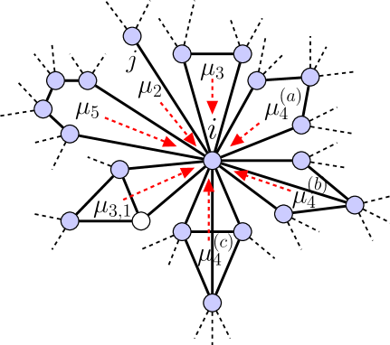
Figure 1: (Color online) Different motifs can be attached to vertex $i$ in a hypergraph: an ordinary edge $a_{ji}$, a triangle, a square, and a pentagon. There are also non-symmetric motifs consisting of four vertices and a clique of size 4. A motif can have internal vertices (open circle) that have edges only inside this motif. Motifs form a locally tree-like hypergraph where they play a role of hyperedges. Arrows represent incoming messages that arrive at vertex $i$ from the motifs attached to this vertex.

One can further generalize equations Eqs. (5) and (6) and introduce the probability $p_{4}(a_{ijkl})$ that vertices $i,j,k,$ and $l$ form a hyperedge of size 4 (a clique or loop of size 4). In the case of loops, one can arrange these vertices in order of increasing vertex index. Then, for a given sequence of squares or cliques, $\{Q_{4}(1),Q_{4}(2),\dots\}$, attached to vertices $i=1,2,\dots$, one can introduce the probability $G_{4}(\{a_{ijkl}\})$ of the realization of a given graph with a given sequence $\{Q_{4}(i)\}$ similar to Eq. (9), and so on. The network ensemble of the configuration model with a given sequences of edges $\{Q_{2}(i)\}$, triangles $\{Q_{3}(i)\}$, squares $\{Q_{4}(i)\}$ and other motifs is described by a product of the corresponding probabilities,

$$G(\{a_{ij}\},\{a_{ijk}\},\{a_{ijkl}\},...)=G_{2}(\{a_{ij}\})G_{3}(\{a_{ijk}\})...$$ (11)

The average of a quantity $K(\{a_{ij}\},\{a_{ijk}\},...)$ over the network ensemble is

$$\langle K\rangle_{\text{en}}=\!\!\!\int K\Bigl{(}\{a_{ij}\},\{a_{ijk}\},\{a_{ijkl}\}...\Bigr{)}\times$$

$$G(\{a_{ij}\},\{a_{ijk}\},\{a_{ijkl}\},...)\prod_{i<j}da_{ij}\!\!\!\prod_{i<j<k}\!\!\!da_{ijk}\!\!\!\!\!\!\prod_{i<j<k<l}\!\!\!\!\!\!da_{ijkl}\dots,$$ (12)

where we integrate over all possible edges and hyperedges.

One can prove that the probability that different motifs have a common edge, i.e., they are overlapping, tends to zero in the infinite size limit $N\rightarrow\infty$. For example, the total number of edges that overlap with triangles equals

$$\left\langle\frac{1}{2}\sum_{i,j,k}a_{ij}a_{ijk}\right\rangle_{\text{en}}=\frac{N\left\langle Q_{2}\right\rangle\left\langle Q_{3}\right\rangle}{N-1}.$$ (13)

This number of double connections is finite in the limit $N\rightarrow\infty$. Because the total number of edges is of the order of $N$, the fraction of double connections tends to zero in the thermodynamic limit. Thus, one can neglect overlapping among different motifs. Using the standard methods in complex network theory Bianconi:bc03 ; Bianconi:bm05a ; Newman:n03b , one can show that in the configuration model the number of finite loops formed by hyperedges is finite in the thermodynamic limit. Therefore, sparse random uncorrelated hypergraphs have a hypertree-like structure.

Uncorrelated random hypergraphs are described by a distribution function $P(Q_{2},Q_{3},Q_{4},\dots)$ which is the probability that a randomly chosen vertex has $Q_{2}$ edges, $Q_{3}$ triangles, $Q_{4}$ squares, and other motifs attached to this vertex. In the case of uncorrelated motifs, we have

$$P(Q_{2},Q_{3},Q_{4},\dots)=\prod_{\ell=2}^{\infty}P_{\ell}(Q_{\ell}).$$ (14)

Here, $P_{\ell}(Q_{\ell})$ is the distribution function of loops of size $\ell$,

$$P_{\ell}(Q_{\ell})=\frac{1}{N}\sum_{i}\delta(Q_{\ell}-Q_{\ell}(i)).$$ (15)

In this kind of network, the number of nearest neighboring vertices of vertex $i$ is equal to

$$Q(i)=Q_{2}(i)+2Q_{3}(i)+2Q_{4}(i)+\dots\,\,.$$ (16)

Therefore, the mean degree is

$$\langle Q\rangle=\frac{1}{N}\sum_{i=1}^{N}Q(i)=\sum_{Q_{2},Q_{3},\dots}QP(Q_{2},Q_{3},Q_{4},\dots).$$ (17)

The local clustering coefficient $C(i)$ of node $i$ with degree $Q(i)$, Eq. (16), is determined by the number of triangles $Q_{3}(i)$ as follows,

$$C(i)=\frac{2Q_{3}(i)}{Q(i)(Q(i)-1)}.$$ (18)

Therefore, $C(i)$ is maximum if a network consists only of triangles. In this case, we have $Q(i)=2Q_{3}(i)$ and therefore

$$C(i)=\frac{1}{Q(i)-1}.$$ (19)

On the other hand, if a network only consists of $\ell$-cliques with a given $\ell$ (fully connected subgraphs of size $\ell$), then the local clustering coefficient of vertex $i$ with $Q_{\ell}(i)$ attached cliques equals

$$C(i)=\frac{\ell-2}{Q(i)-1},$$ (20)

where $Q(i)=(\ell-1)Q_{\ell}(i)$ is degree of vertex $i$. If other motifs (edges, squares, and larger finite loops) are present in the network, then according to Eqs. (18) and (20) the local clustering coefficient $C(i)$ is smaller than $(\ell-2)/[Q(i)-1]$. In Refs. Serrano2006a ; Serrano2006b ; Serrano2006c , it was shown that properties of networks with ”weak clustering”, $C(Q)\sim O(1/Q)$, may differ from properties of networks with ”strong clustering” when $C(Q)$ decreases slower than $1/Q$. The latter networks are beyond the scope of the present article.

III Belief-propagation algorithm

Let us consider the Ising model with pairwise interactions between nearest neighboring spins on a sparse random network with arbitrary distributions of motifs. The Hamiltonian of the model is

$$E= -\sum_{i}H_{i}S_{i}-\sum_{i<j}a_{ij}J_{ij}S_{i}S_{j}$$

$$-\sum_{i<j<k}a_{ijk}(J_{ij}S_{i}S_{j}+J_{jk}S_{j}S_{k}+J_{ik}S_{i}S_{k})$$

$$-\!\!\!\sum_{i<j<k<l}\!\!\!a_{ijkl}(J_{ij}S_{i}S_{j}+J_{jk}S_{j}S_{k}+J_{kl}S_{k}S_{l}+\dots)$$

$$+...~{}.$$ (21)

Here we sum the energies of spin clusters corresponding to motifs in the network. The second sum corresponds to simple edges. The third sum corresponds to triangles. The forth sum corresponds to motifs of size 4, and so on. $H_{i}$ is a local magnetic field at vertex $i$. The coupling $J_{ij}$ determines the energy of pairwise interaction between spins $i$ and $j$. In general, one can introduce multi-spin interactions between spins in hyperedges, for example, $S_{i}S_{j}S_{k}$, $S_{i}S_{j}S_{k}S_{l}$, and so on. However, this kind of interaction is beyond the scope of our article. Generally, the local fields $H_{i}$ and the couplings $J_{ij}$ can be random quantities.

In order to solve this model, we generalize the belief-propagation algorithm. At first, we note the belief-propagation algorithm in application for the Ising model on tree-like uncorrelated complex networks without short loops (for more details, see Ref. Dorogovtsev:dgm08 ). In this case, there are only edges determined by the adjacency matrix $a_{ij}$ and the clustering coefficient is zero in the thermodynamic limit. Consider spin $i$. A nearest neighboring spin $j$ sends a so-called message to spin $i$ that we denote as $\mu_{ji}(S_{i})$. This message is normalized,

$$\sum_{S_{i}=\pm 1}\mu_{ji}(S_{i})=1.$$ (22)

Within the belief-propagation algorithm, the probability that spin $i$ is in a state $S_{i}$ is determined by the normalized product of incoming messages to spin $i$ and the probabilistic factor $e^{\beta H_{i}S_{i}}$ due to a local field $H_{i}$:

$$p_{i}(S_{i})=\frac{1}{A}e^{\beta H_{i}S_{i}}\prod_{j}\mu_{ji}(S_{i}),$$ (23)

where $A$ is a normalization constant and $\beta=1/T$ is the reciprocal temperature. Now we can calculate the mean moment of spin $i$,

$$\langle S_{i}\rangle=\sum_{S_{i}=\pm 1}S_{i}p_{i}(S_{i}).$$ (24)

A message $\mu_{ji}(S_{i})$ can be written in a general form,

$$\mu_{ji}(S_{i})=\exp(\beta h_{ji}S_{i})/[2\cosh(\beta h_{ji})],$$ (25)

Using this representation, we rewrite Eq. (24) in a physically clear form,

$$\langle S_{i}\rangle=\tanh\Bigl{(}\beta H_{i}+\beta\sum_{j}a_{ji}h_{ji}\Bigr{)}.$$ (26)

This equation shows that a parameter $h_{ji}$ plays the role of an effective field produced by spin $j$ at site $i$. Messages $\mu_{ji}(S_{i})$ obey a self-consistent equation that is called update rule,

$$B\sum_{S_{j}=\pm 1}e^{-\beta E(j,i)}\prod_{n\neq i}\mu_{nj}(S_{j})=\mu_{ji}(S_{i}),$$ (27)

where the index $n$ numerates nearest neighbors of vertex $j$ and $B$ is a normalization constant. The diagram representation of this equation is shown in Fig. 2 $(a)$. The probabilistic factor $\exp[-\beta E(j,i)]$ takes account of the interaction energy of spins $j$ and $i$ and a local field $H_{j}$,

$$E(j,i)=-H_{j}S_{j}-a_{ji}J_{ji}S_{i}S_{j}.$$ (28)

Thus, a message from $j$ to $i$ is determined by the coupling between these spins and messages received by $j$ from its neighbors except $i$. Multiplying Eq. (27) by $S_{i}$ and summing over $S_{i}=\pm 1$, we obtain a self-consistent equation for the effective fields $h_{ji}$,

$$\tanh(\beta h_{ji})=\tanh\Bigl{(}\beta a_{ji}J_{ji}\Bigr{)}\tanh\Bigl{[}\beta(H_{j}+\!\sum_{n(\neq i)}\!a_{nj}h_{nj})\Bigr{]}.$$ (29)

In the thermodynamic limit, this equation is exact for a tree-like graph. The Bethe-Peierls approach and the Baxter recurrence method give exactly the same result Dorogovtsev:dgm08 ; bbook82 . In numerical calculations, Eqs. (27) and (29) may be solved by use of iterations. In a general case, an analytical solution of these equations is unknown. In the case of all-to-all interactions with random couplings $J_{ji}$ (the Sherrington-Kirkpatrick model), this set of equations is reduced to well-known TAP equations Thouless:tap77 that are exact in the thermodynamic limit. These equations also give an exact solution of the ferromagnetic Ising model with uniform couplings $J_{ji}=J>0$ on a random uncorrelated graph with zero clustering coefficient dgm02 ; lvvz02 ; Dorogovtsev:dgm08 .

Figure 2: Diagram representation of the belief-propagation update rules for messages from a motif to a destination vertex $i$. Arrows represent incoming messages. [(a), (b) and (c)] Update rules for an edge, a triangle, and a square. Mathematical expressions of these diagrams are given by Eqs. (27) and (33).

We now generalize the belief-propagation algorithm to the case of networks with given distributions of motifs described in Sec. II. In a network that consists only of edges, a message goes along an edge from the spin at one edge end to the spin at the other edge end. For the networks with motifs, it is natural to introduce a message that is sent by a motif attached to a vertex. This message goes to a spin to which this motif (hyperedge) is attached. Different motifs may be attached to a vertex, see Fig. 1. Let $M_{\ell}(i)$ denote a cluster of size $\ell$ attached to vertex $i$ that we will call the destination vertex. Vertices $j_{1},j_{2},...,j_{\ell-1}$ together with the destination vertex $i$ form this motif. We introduce a message $\mu_{M_{\ell}(i)}(S_{i})$ to spin $i$ from a motif $M_{\ell}(i)$. This message is normalized and can be written as follows,

$$\mu_{M_{\ell}(i)}(S_{i})=\exp\Bigl{(}\beta h_{M_{\ell}(i)}S_{i}\Bigr{)}/[2\cosh(\beta h_{M_{\ell}(i)})].$$ (30)

As above, the probability that spin $i$ is in a state $S_{i}$ is determined by the normalized product of incoming messages from motifs attached to spin $i$ and the probabilistic factor $e^{\beta H_{i}S_{i}}$,

$$p_{i}(S_{i})=\frac{1}{A}e^{\beta H_{i}S_{i}}\prod_{\{M_{\ell}(i)\}}\mu_{M_{\ell}(i)}(S_{i}).$$ (31)

Using Eq. (24), we find that the mean moment $\langle S_{i}\rangle$ is determined by effective fields $h_{M_{\ell}(i)}$ acting on spin $i$ from motifs $M_{\ell}(i)$, $\ell=2,3,4,...$, attached to $i$, see Fig. 1,

$$\langle S_{i}\rangle=\tanh\Bigl{(}\beta H_{i}+\beta\sum_{\{M_{\ell}(i)\}}h_{M_{\ell}(i)}\Bigr{)}.$$ (32)

Here the sum is taken over motifs attached to $i$.

Let us find an update rule for a message $\mu_{M_{\ell}(i)}(S_{i})$ from a given motif $M_{\ell}(i)$ to vertex $i$. We introduce the following update rule:

$$B\!\!\!\!\sum_{\{S_{j}=\pm 1\}}\!\!\!\!e^{-\beta E(M_{\ell}(i))}\prod_{j}\!\prod_{\{M_{n}(j)\neq M_{\ell}(i)\}}\!\!\!\!\!\!\!\!\!\!\!\mu_{M_{n}(j)}(S_{j})=\!\mu_{M_{\ell}(i)}(S_{i}).$$ (33)

This rule shows that the message $\mu_{M_{\ell}(i)}(S_{i})$ is equal to the product of incoming messages from motifs attached to all spins $j$ in the motif $M_{\ell}(i)$ except spin $i$ and the motif $M_{\ell}(i)$ itself (see Fig. 2. In Eq. (33) we average over all spin configurations of the spins $S_{j_{1}},S_{j_{2}},...$, and $S_{j_{\ell-1}}$ in the motif. $B$ is a normalization constant. $E[M_{\ell}(i)]$ is an energy of the interaction between spins in the motif $M_{\ell}(i)$. This update rule also takes account of local fields $H_{j}$ acting on all spins except the destination spin $i$. We note that Eq. (33) is valid for arbitrary motifs even with a complex internal structure. The only assumption is that a sparse network under consideration, in terms of hypergraphs, has a hypertree-like structure. Messages can be found numerically by use of iterations of Eq. (33) that start from an initial distribution of the messages.

For the sake of simplicity, let motifs $M_{\ell}(i)$ be finite loops of size $\ell=2,3,\dots$. Then

$$E(M_{\ell}(i))=-\sum_{n=1}^{\ell-1}H_{j_{n}}S_{j_{n}}-\sum_{n=0}^{\ell-1}J_{j_{n}j_{n+1}}S_{j_{n}}S_{j_{n+1}},$$ (34)

where $j_{0}=j_{\ell}\equiv i$. If motifs are $\ell$-cliques, then the energy $E(M_{\ell}(i))$ takes account of interactions between all spins in these cliques,

$$E(M_{\ell}(i))=-\sum_{j(\neq i)}H_{j}S_{j}-\frac{1}{2}\sum_{i,j\in M_{\ell}(i)}J_{i,j}S_{i}S_{j}\text{.}$$ (35)

Multiplying Eq. (33) by $S_{i}$ and summing over all spin configurations, we obtain an equation for the effective field $h_{M_{\ell}(i)}$,

$$\tanh\Bigl{(}\beta h_{M_{\ell}(i)}\Bigr{)}=\langle S_{i}\rangle_{M_{\ell}(i)}.$$ (36)

The function on the right hand side is

$$\langle S_{i}\rangle_{M_{\ell}(i)}=\frac{1}{Z(M_{\ell}(i))}\sum_{\{S_{i},S_{j_{1}},...=\pm 1\}}\!\!\!\!S_{i}e^{-\beta\widetilde{E}(M_{\ell}(i))}\text{.}$$ (37)

This function has a meaning of the mean moment of spin $S_{i}$ in the cluster $M_{\ell}(i)$ with an energy

$$\widetilde{E}(M_{\ell}(i))=-\sum_{n=1}^{\ell-1}H_{t}(j_{n})S_{j_{n}}-\sum_{n=0}^{\ell}J_{j_{n}j_{n+1}}S_{j_{n}}S_{j_{n+1}}\text{.}$$ (38)

This energy takes into account both the interaction between spins in this motif and total effective fields $H_{t}(j)$ acting on these spins. In turn, the field $H_{t}(j)$ acting on $j$ is the sum of a local field $H_{j}$ and effective fields $h_{M_{m}(j)}$ produced by incoming messages from motifs $M_{m}(j)$ attached to vertex $j$ except the motif $M_{\ell}(i)$, see Fig. 3,

$$H_{t}(j)=H_{j}+\sum_{\{M_{m}(j)(\neq M_{\ell}(i))\}}h_{M_{m}(j)}.$$ (39)

$Z[M_{\ell}(i)]$ is the partition function of the cluster $M_{\ell}(i)$,

$$Z[M_{\ell}(i)]=\sum_{\{S_{i},S_{j_{1}},...=\pm 1\}}e^{-\beta\widetilde{E}(M_{\ell}(i))}.$$ (40)

Thus, the function $\langle S_{i}\rangle_{M_{\ell}(i)}$ is a function $F[H_{t}(j_{1}),H_{t}(j_{2}),\dots,H_{t}(j_{\ell-1})]$ of the total fields $H_{t}(j)$ acting on all spins in the motif $M_{\ell}(i)$ except spin $i$. For a given network with motifs, it is necessary to solve Eq. (36) with respect to the effective fields $h_{M_{\ell}(i)}$. One then can calculate the mean magnetic moments $\langle S_{i}\rangle$ from Eq. (32). Note that the only condition we used to derive the equations above was hypertree-like structure of the networks. The absence of correlations in these hypertree-like networks was not needed. Equations (33) and  (36) are our main result that actually generalizes the Bethe-Peierls approach and the Baxter recurrence method.

Let us study the ferromagnetic Ising model with uniform couplings, $J_{ji}=J>0$, at zero magnetic field, i.e., $H_{i}=H=0$, on a uncorrelated hypergraph which consists of edges and finite loops. In a random network, effective fields $h_{M_{\ell}(i)}$ are also random variable and fluctuate from vertex to vertex. For a given $\ell$, we introduce the distribution function of fields $h_{M_{\ell}(i)}$,

$$\Psi_{\ell}(h)=\frac{1}{A}\sum_{i=1}^{N}\sum_{\{M_{\ell}(i)\}}\delta(h-h_{M_{\ell}(i)}).$$ (41)

Here, we sum over vertices $i$ and attached motifs $M_{\ell}(i)$ of size $\ell$. $A=N\langle Q_{\ell}\rangle$ is the normalization constant. We assume that in the thermodynamic limit, $N\rightarrow\infty$, the average over vertices in the network is equivalent to the average over the statistical network ensemble, Eq. (12). Using Eq. (36), we obtain an equation for the distribution function $\Psi_{\ell}(h)$,

$$\Psi_{\ell}(h)=\int\delta\Bigl{(}h-T\tanh^{-1}[\langle S\rangle_{M_{\ell}}]\Bigr{)}\prod_{j=1}^{\ell-1}\Phi_{\ell}(H_{t}(j))dH_{t}(j).$$ (42)

Here $\langle S\rangle_{M_{\ell}}$ is the function $F[H_{t}(1),H_{t}(2),\dots,H_{t}(\ell-1)]$ defined by Eq. (37). $H_{t}(j)$ is a total field, Eq. (39), acting on vertex $j=1,2,\dots,\ell-1$ in the motif $M_{\ell}$, see Fig. 3. The integration is over fields $H_{t}(j)$ with the distribution function $\Phi_{\ell}(H_{t}(j))$. Using Eq. (39), we can find this function,

$$\Phi_{\ell}(H)=\sum_{Q_{2},Q_{3},...}\!\!\!P(Q_{2},Q_{3},...)\frac{Q_{\ell}}{\langle Q_{\ell}\rangle}\times$$

$$\int\delta\Bigl{(}H-\!\!\!\sum_{m(\neq\ell)}^{\infty}\sum_{\alpha=1}^{Q_{m}}h_{M_{m}}(\alpha)-\!\!\!\sum_{\alpha=1}^{Q_{\ell}-1}h_{M_{\ell}}(\alpha)\Bigr{)}\times$$

$$\prod_{m(\neq\ell)}^{\infty}\!\!\Bigl{(}\prod_{\alpha=1}^{Q_{m}}\!\!\Psi_{m}(h_{M_{m}}(\alpha))dh_{M_{m}}(\alpha)\Bigr{)}\!\!\!\!\prod_{\alpha=1}^{Q_{\ell}-1}\!\!\Psi_{\ell}(h_{M_{\ell}}(\alpha))dh_{M_{\ell}}(\alpha).$$

Here $P(Q_{2},Q_{3},...)$ is given by Eq. (14). This is the probability that a destination vertex has $Q_{2}$ edges, $Q_{3}$ triangles, and so on. In turn, incoming messages $h_{M_{m}}(\alpha)$ to the destination spin from attached loops of size $m$ are numerated by the index $\alpha$, $\alpha=1,2,...,Q_{m}$. Only for incoming messages from loops of size $\ell$ do we have $\alpha=1,2,...,Q_{\ell}-1$, because we should not account for the motif $M_{\ell}$. The integration is over incoming messages to all vertices in the motif (hyperedge) $M_{\ell}$ except the destination vertex $i$, see Fig. 3. Note that we have an additional factor $Q_{\ell}/\langle Q_{\ell}\rangle$, because there is the probability in the configuration model $P_{\ell}(Q_{\ell})Q_{\ell}/\langle Q_{\ell}\rangle$ that if we arrive at a destination vertex along a hyperedge $M_{\ell}$, then this vertex has $Q_{\ell}-1$ outgoing hyperedges $M_{\ell}$. Equations  (42) and  (LABEL:phi) represent a set of self-consistent equations for the functions $\Psi_{\ell}(h)$, $\ell=2,3,4,\dots\,$. Using Eq. (32), one then can find a distribution function of spontaneous magnetic moments $\langle S_{i}\rangle$ in the network. Equations  (42) and  (LABEL:phi) are also valid for networks with cliques.

Figure 3: (a) A loop (motif $M_{\ell}$) of size $\ell$ is attached to destination vertex $i$. Wave arrows represent total effective fields $H_{t}(j)$ acting on spins with index $j=1,2,\dots,\ell-1$ in this loop. (b) In turn, the total effective field $H_{t}(j)$ is a sum of effective fields produced by all motifs attached to vertex $j$ except the motif $M_{\ell}$. There are $Q_{2}(j)$ edges, $Q_{3}(j)$ triangles, and so on. However, the number of loops of size $\ell$ equals $Q_{\ell}(j)-1$, because we should not account the motif $M_{\ell}$ that is common for vertices $j$ and $i$.

It should be noted that our approach is similar to the generalized belief-propagation algorithm proposed in Ref. Yedidia:yfw01 . It was shown that the belief-propagation algorithm is equivalent to the cluster variation method (CVM) introduced by R. Kikuchi (see Ref. Pelizzola05 for more details). Note that in the model of complex networks in the present work, two motifs can only overlap each other by a single node. They have no joint links. Motifs here play the role of “hyperedges” in contrast to the approach in Ref. Yedidia:yfw01 where clusters are considered as “super-nodes”. Finally, we assumed that networks under consideration have a hypertree-like structure in the infinite size limit.

IV Critical temperature and critical behavior

In the paramagnetic phase at zero magnetic field, there is no spontaneous magnetization and the effective fields are equal to zero, i.e., $h_{M_{\ell}}=0$. Therefore, we obtain

$$\Psi_{\ell}(h)=\delta(h).$$ (44)

for any $\ell$. This is the only solution of Eqs. (42) and  (LABEL:phi) in the paramagnetic phase. Below a critical temperature $T_{c}$, this solution becomes unstable and a non-trivial solution for the function $\Psi_{\ell}(h)$ emerges. In this case, a mean value of the effective field $h_{M_{\ell}}$,

$$\langle h_{M_{\ell}}\rangle_{T}=\int h\Psi_{\ell}(h)dh,$$ (45)

becomes non-zero. Here $\langle...\rangle_{T}$ denotes the thermodynamic average. In the case of a continuous phase transition, $\langle h_{M_{\ell}}\rangle_{T}$ tends to zero if the temperature $T$ tends to $T_{c}$ from below. Let use this fact. From Eq. (36) we obtain

$$\int\tanh(\beta h)\Psi_{\ell}(h)dh=\int\langle S\rangle_{M_{\ell}}\prod_{j=1}^{\ell-1}\Phi_{\ell}(H_{t}(j))dH_{t}(j).$$ (46)

We expand the functions $\tanh(\beta h)$ and $\langle S\rangle_{M_{\ell}}$ on the left and right hand sides of this equation in small $h$ and $H_{t}(j)$, respectively:

$$\tanh(\beta h)=\beta h+O(h^{3}),$$

$$\langle S_{i}\rangle_{M_{\ell}}=\sum_{j=1}^{\ell-1}\chi_{\ell}(ij)H_{t}(j)+O(H_{t}^{3}(j)),$$ (47)

where we define

$$\chi_{\ell}(ij)\equiv\frac{\partial\langle S_{i}\rangle_{M_{\ell}}}{\partial H_{t}(j)}\Big{|}_{H_{t}(j)=0}=\beta\langle S_{i}S_{j}\rangle_{M_{\ell}}\Big{|}_{H_{t}(j)=0}.$$ (48)

$\chi_{\ell}(ij)$ is a non-local susceptibility in a spin cluster ${M_{\ell}}$ at zero magnetic field. Note that $T\chi_{\ell}(ii)=1$. Assuming that at $T\rightarrow T_{c}-0$ the first moment of the function $\Psi_{\ell}(h)$, i.e., $\langle h_{M_{m}}\rangle_{T}$, is much larger than higher moments, i.e., $\langle h_{M_{m}}\rangle_{T}\gg\langle h_{M_{m}}^{n}\rangle_{T}$, in the leading order we obtain a linear equation,

$$\langle h_{M_{\ell}}\rangle_{T}=\frac{F_{\ell}(T)}{\langle Q_{\ell}\rangle}\Bigl{[}\langle Q_{\ell}(Q_{\ell}-1)\rangle\langle h_{M_{\ell}}\rangle_{T}$$

$$+\sum_{m(\neq\ell)}^{\infty}\langle Q_{\ell}Q_{m}\rangle\langle h_{M_{m}}\rangle_{T}\Bigr{]},$$ (49)

where $\langle\dots\rangle$ defines an average over the distribution function $P(Q_{2},Q_{3},Q_{4},\dots)$ given by Eq. (14). The function $F_{\ell}(T)$ is defined as follows,

$$F_{\ell}(T)\equiv T\sum_{j=1}^{\ell-1}\chi_{\ell}(ij)=T\chi_{\ell}-1,$$ (50)

$\chi_{\ell}$ is the total zero-field magnetic susceptibility of the Ising model on a ring of size $\ell$. Simple calculations give

$$F_{2}(T)=t,\,\,\,\,\,\,\,\,\,\,\ell=2,$$

$$F_{\ell}(T)=\frac{2t(1-t^{\ell-1})}{(1-t)(1+t^{\ell})},\,\,\,\,\,\,\,\,\,\,\ell\geq 3,$$ (51)

where $t=\tanh(J/T)$. In the paramagnetic phase, the set of linear equations (49) for parameters $\langle h_{M_{\ell}}\rangle_{T}$ has only a trivial solution, $\langle h_{M_{\ell}}\rangle_{T}=0$. A non-trivial solution appears at a temperature at which

$$det\widehat{M}=0,$$ (52)

where the matrix $M_{mn}$ is defined as follows:

$$M_{mn}=\langle Q_{m}Q_{n}\rangle,\,\,\,\,\,\,\,\,\,\,m\neq n,$$

$$M_{mm}=\langle Q_{m}(Q_{m}-1)\rangle-\frac{\langle Q_{m}\rangle}{F_{m}(T)},$$ (53)

for $m,n=2,3,...\,$. Equation (52) determines the critical point $T_{c}$ of the continuous phase transition. Below $T_{c}$, spontaneous effective fields appear, i.e., $\langle h_{M_{\ell}}\rangle_{T}\neq 0$. Therefore, there is a non-zero spontaneous magnetic moment. If all motifs are loops of equal length $\ell$, then the critical temperature $T_{c}$ is determined by the equation

$$B_{\ell}F_{\ell}(T)=1$$ (54)

where $B_{\ell}$ is the average branching coefficient for these hyperedges ($\ell$-loops in this network),

$$B_{\ell}=\frac{\langle Q_{\ell}(Q_{\ell}-1)\rangle}{\langle Q_{\ell}\rangle}.$$ (55)

In particular, if there are only edges, i.e., $\ell=2$, then Eq. (54) gives

$$T_{c}=2J/\ln\Bigl{(}\frac{B_{2}+1}{B_{2}-1}\Bigr{)}.$$ (56)

This result was found for uncorrelated random complex networks with arbitrary degree distributions dgm02 ; lvvz02 ; Dorogovtsev:dgm08 . In the limit $B_{\ell}\gg 1$, we find that

$$T_{c}(\ell=2)/J\cong B_{\ell}+o(1),$$ (57)

$$T_{c}(\ell\geq 3)/J\cong 2B_{\ell}+1+o(1),$$ (58)

Figure 4 shows the dependence of the critical temperature $T_{c}(\ell)$ on the mean number of nearest neighbors $\langle Q\rangle$ in the networks with the Poissonian distribution of $\ell$-loop motifs. In this case the average branching coefficient is $B_{\ell}=Q_{\ell}$. Notice also that at $\ell\geq 3$ we have $\langle Q\rangle=2\langle Q_{\ell}\rangle=2B_{\ell}$ according to Eqs. (16) and (17). Comparison between Eqs. (57) and (58) shows that at a given mean degree $Q\gg 1$ for the Poisson distribution of hyperdegrees the critical temperature $T_{c}(\ell>2)$ is higher than $T_{c}(\ell=2)$ only by 1. This shift is the only effect of finite loops.

If there are only two motifs, for example, loops of size $\ell$ and $\ell^{\prime}$, then Eq. (52) leads to the equation

$$\Bigl{[}B_{\ell}-\frac{1}{F_{\ell}(T)}\Bigr{]}\Bigl{[}B_{\ell^{\prime}}-\frac{1}{F_{\ell^{\prime}}(T)}\Bigr{]}=\frac{\langle Q_{\ell}Q_{\ell^{\prime}}\rangle^{2}}{\langle Q_{\ell}\rangle\langle Q_{\ell^{\prime}}\rangle}.$$ (59)

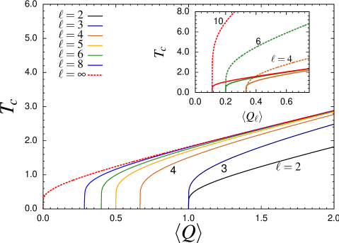
Figure 4: (Color online) Critical temperature $T_{c}$ of the ferromagnetic Ising model versus the mean number of nearest neighbors $\langle Q\rangle=2\langle Q_{\ell}\rangle$ in uncorrelated random networks with Poisson distribution of loops of size $\ell$ and the mean number $\langle Q_{\ell}\rangle$ of these loops attached to a vertex. Note that the case $\ell=2$ is special: there are no loops, and we have the Erdős-Rényi graph. Inset displays $T_{c}$ versus the mean number $\langle Q_{\ell}\rangle$ of $\ell$-cliques (dashed lines), and, for comparison, $T_{c}$ for finite loops of the same size $\ell$ (solid lines). Here we set $J=1$.

From Eqs. (51) and (54), it follows that if an uncorrelated random hypergraph has a divergent second moment $\langle Q_{m}^{2}\rangle$ for any $m\geq 2$, then $T_{c}$ becomes infinite in the infinite size limit. This result was obtained for ordinary uncorrelated random complex network in Refs. dgm02 ; lvvz02 ; Dorogovtsev:dgm08 .

Another example of complex motifs are $\ell$-cliques. In this kind of complex networks the clustering coefficient is larger than in networks with loops of size $\ell=3$ (compare between Eqs. (19) and (20)). Calculating the susceptibility $\chi$ of a cluster of spins on this subgraph, we can find the function $F_{\ell}(T)$ in Eq. (50) at $\ell\geq 3$,

$$F_{\ell}(T)=(\ell-1)\Bigl{[}1-\frac{4I_{\ell-2}(T)}{I_{\ell}(T)}\Bigr{]}.$$ (60)

Here we introduced the function

$$I_{\ell}(T)=\sum_{n=0}^{\ell}C_{n}^{\ell}\exp\Bigr{[}\frac{1}{2}\beta J(2n-\ell)^{2}\Bigl{]},$$ (61)

where $C_{n}^{\ell}=n!/(n-\ell)!\ell!$ is the binomial coefficient. If a network only consists of uncorrelated $\ell$-cliques then the critical temperature of the ferromagnetic Ising model is given by Eq. (54) with the function Eq. (60). In the limit $B_{\ell}\gg 1$ we obtain an asymptotic result,

$$T_{c}\approx(\ell-1)B_{\ell}+(\ell-2)(1+o(1)).$$ (62)

Let us consider the Poisson distribution. In this case we have $B_{\ell}=\langle Q_{\ell}\rangle$ and the mean degree is $\langle Q\rangle=(\ell-1)\langle Q_{\ell}\rangle=(\ell-1)B_{\ell}$. Critical temperatures of networks with $\ell-$cliques and $\ell-$loops are compared in Fig. 4. Comparison between Eqs. (62), (57) and (58) shows that at a given mean degree $\langle Q\rangle\gg 1$ the critical temperature $T_{c}(\ell)$ in Eq. (62) is larger than the critical temperature Eq. (57) only by $\ell-2$. This shift is the only effect of clustering. It gives a relative correction of order $O[(\ell-2)/\langle Q\rangle]$, because $T_{c}(\ell)/T_{c}(\ell=2)\approx 1+(\ell-2)/\langle Q\rangle$. This result shows that the internal structure of motifs may change the critical temperature of the Ising model although the percolation threshold may be the same (see below).

Thus in the considered random networks the average branching coefficient $B_{\ell}$ is crucially important. If $B_{\ell}\gg 1$, clustering and finite loops lead to a relatively small shift of the critical temperature in comparison to networks without loops but with the same average branching coefficient. However, in networks with a small branching coefficient of motifs, influence of clustering and finite loops is stronger. Indeed, at $\ell=2$ the critical temperature, Eq. (56), exceeds zero, $T_{c}>0$, if the average branching coefficient $B_{2}>1$ (for the Poisson distribution this corresponds to the mean degree $\langle Q\rangle>1$). This is due to the fact that only in this case there is a giant connected component [see Eq. (67)]. In networks with finite loops of size $\ell$, the percolation threshold from Eq. (67) is $B_{\ell}=1/(\ell-1)$. Therefore, the phase transition appears at the average branching coefficient $B_{\ell}=1/(\ell-1)$ which is much smaller than 1 if $\ell\gg 1$ (for the Poisson distribution this corresponds to the mean degree $\langle Q\rangle>2/(\ell-1)\ll 1$).

Does clustering influence the critical behavior in the network with motifs? In order to answer this question we consider networks that consist of cliques of a given size $\ell$ with the mean number $\langle Q_{\ell}\rangle$ of $\ell-$cliques attached to a node. It is convenient to assume that the distribution function $P_{\ell}(Q_{\ell})$ of $\ell-$cliques has the following asymptotic behavior: $P_{\ell}(Q_{\ell})\propto 1/Q_{\ell}^{\gamma}$. In Eq. (LABEL:phi), we use the ”effective medium” approximation introduced in Ref. dgm02 :

$$\sum_{\alpha=1}^{Q_{\ell}-1}h_{M_{\ell}}(\alpha)\approx(Q_{\ell}-1)\langle h_{M_{\ell}}\rangle_{T}$$ (63)

where $\langle h_{M_{\ell}}\rangle_{T}$ is the mean effective field acting on a node from an attached $\ell$-clique. As was shown in Ref. dgm02 , this approximation takes into account the most dangerous highly connected nodes and gives exact critical behavior for random uncorrelated tree-like networks (see also Refs. lvvz02 ; Dorogovtsev:dgm08 ). As a result, we obtain the distribution function $\Phi_{\ell}(H)$ of the total field $H$ acting on a node from attached $\ell$-cliques as a function of $\langle h_{M_{\ell}}\rangle_{T}$,

$$\Phi_{\ell}(H)\approx\sum_{Q_{\ell}}P_{\ell}(Q_{\ell})\frac{Q_{\ell}}{\langle Q_{\ell}\rangle}\delta\Bigl{(}H-(Q_{\ell}-1)\langle h_{M_{\ell}}\rangle_{T}\Bigr{)}.$$ (64)

Substituting Eqs. (42) and (LABEL:phi) into Eq. (45), we obtain a self consistent equation for the mean effective field $\langle h_{M_{\ell}}\rangle_{T}$,

$$\langle h_{M_{\ell}}\rangle_{T}=G(\langle h_{M_{\ell}}\rangle_{T}),$$ (65)

where $G(\langle h_{M_{\ell}}\rangle_{T})$ is the right hand side of Eq. (45). Critical behavior of the model is determined by analytical behavior of the function $G(h)$ at small $h$ dgm02 . Analysis of analytical properties of the function $G(\langle h_{M_{\ell}}\rangle_{T})$ at zero magnetic field shows that if the forth moment of degree distribution is finite, i.e., $\langle Q_{\ell}^{4}\rangle\equiv\sum_{Q_{\ell}}P_{\ell}(Q_{\ell})Q_{\ell}^{4}<\infty$ (scale-free networks with the degree exponent $\gamma>5$), then $G(h)=Ah+Bh^{3}+o(h^{3})$ where $A$ and $B$ are certain functions of temperature $T$. Solving Eq. (65), we find that the spontaneous magnetization $m(T)$ and the mean effective field $\langle h_{M_{\ell}}\rangle_{T}$ behave as $m(T)\propto\langle h_{M_{\ell}}\rangle_{T}\propto(T_{c}-T)^{\beta}$ below $T_{c}$ with the standard mean-field exponent $\beta=1/2$. If $\langle Q_{\ell}^{4}\rangle$ diverges but the second moment $\langle Q_{\ell}^{2}\rangle$ is finite (scale-free networks with $3<\gamma\leq 5$) then $G(h)=Ah+B^{\prime}h^{\gamma-2}+o(h^{\gamma-2})$. In this case, the critical exponent $\beta$ becomes dependent on the asymptotic behavior of the distribution function $P_{\ell}(Q_{\ell})$, namely, $\beta=1/(\gamma-3)$. Finally, if $\langle Q_{\ell}^{2}\rangle$ diverges but the mean degree $\langle Q_{\ell}\rangle$ is finite (scale-free networks with $2<\gamma\leq 3$), then in the thermodynamic limit the critical temperature $T_{c}$ tends to infinity, i.e., at any finite temperature the Ising model is in the ordered phase. This is the critical behavior that was found for the ferromagnetic Ising model on random uncorrelated complex networks dgm02 ; lvvz02 ; Dorogovtsev:dgm08 .

Our approach is explicit for sparse random networks that have local hypertree-like structure. Two motifs can only overlap each other by a single node. If two clusters have common edges, one can combine them and introduce a new motif. The internal structure of motifs does not influence the critical behavior of the ferromagnetic Ising model. However this structure may be essential for models with frustrations (spin glasses). Relaxing the hypertree-like assumption may change crucially the critical behavior of the Ising model. Furthermore, as we have showed above, asymptotic behavior of distribution function of motifs is significant for the critical behavior of the Ising model and other models of statistical physics on complex networks Dorogovtsev:dgm08 . In our analysis of critical behavior we also assumed that there are no correlations in the distribution of motifs over a network. The role of degree-degree correlations in critical behavior for percolation on complex networks was demonstrated in Ref. gdm08 . Weak clustering in the sense of Sec. II does not influence the critical behavior of the Ising model. The influence of strong clustering demands further investigation.

V Percolation threshold

Equation (52) permits us to find the percolation threshold in these loopy networks. Below the percolation threshold, a network consists of finite clusters and there is no giant component. In this case, there is no phase transition in the Ising model. This spin system is in a paramagnetic state at any $T$. At a point of the birth of a giant component, there is a giant connected cluster and the critical temperature is $T_{c}=0$. Above the percolation threshold, the critical temperature is non-zero, $T_{c}>0$. Therefore, in a general case for an arbitrary distribution function $P(Q_{2},Q_{3},Q_{4},...)$, the percolation point is determined by Eq. (52) at $T=0$. In this case, we have $F_{\ell}(T=0)=\ell-1$. For example, if there are only loops of size $\ell$ and $\ell^{\prime}$ then Eq. (59) takes a form,

$$\Bigl{[}B_{\ell}-\frac{1}{\ell-1}\Bigr{]}\Bigl{[}B_{\ell^{\prime}}-\frac{1}{\ell^{\prime}-1}\Bigr{]}=\frac{\langle Q_{\ell}Q_{\ell^{\prime}}\rangle^{2}}{\langle Q_{\ell}\rangle\langle Q_{\ell^{\prime}}\rangle}.$$ (66)

In the case of $\ell$-loop motifs, Eq. (54) gives the following criterion for the birth of a giant connected component:

$$(\ell-1)B_{\ell}=1,$$ (67)

where $B_{\ell}$ is the average branching. At $\ell=2$, this is the Molloy-Reed criterion for ordinary uncorrelated random networks mr95 . The percolation threshold can be seen in Fig. 4 as a critical value of the mean degree $\langle Q\rangle$, Eq. (17), below which $T_{c}$ is zero. Our results about the percolation threshold agree with results obtained in Refs. newman:n09 ; kn10b ; hmg2010 by use of different approaches. It is interesting that we have $F_{\ell}(T=0)=\ell-1$ for both finite loops and cliques of the same size $\ell$. Therefore, the percolation threshold Eq. (67), i.e., the point of birth of the giant component, is also the same.

VI Application to real networks

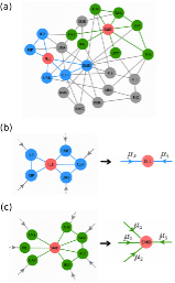
Figure 5: (Color online) (a) Small network of motoneurons in C. elegans (adapted from Fig. 21(c) in Ref. white86 ). In this figure we follow notations of neurons used in Ref. white86 . [(b) and (c)] Two subgraphs formed by two nodes IL1 and SMD (red circles) and their nearest neighbors. (b) The node IL1 has two attached motifs, one triangle and one square. In (c) the node SMD has three simple edges and one attached pentagon. Messages sent by these motifs are shown schematically by arrows on the right-hand side.

As was mentioned in Sec. I, real networks are clustered and display network motifs ab01a ; dm01c ; Dorogovtsev:2010 ; Newman:n03a ; Milo2002 ; Milo2004 ; Sporn2004 ; Alon2007 . The ordinary belief-propagation algorithm can give only approximate results for this kind of network. One can improve this approach by use of the generalized belief-propagation algorithm introduced in Sec. III. For this purpose, one should, first, detect motifs attached to each node in a network. As an example we chose a small network of motoneurons in the nervous systems of Caenorhabditis elegans white86 . The undirected version of this network is shown in Fig. 5(a). Nodes and links represent neurons and synaptic connections, respectively. In order to detect motifs, we propose the following method. Choose a node and consider a subgraph formed by this node and its nearest neighbors. Only links between nodes in this subgraph are taken into account. The obtained subgraph can be represented as a set of clusters (motifs) overlapping only at the chosen node. Two examples of subgraphs are shown in Figs. 5(b) and 5(c). One can see that motifs attached to the chosen nodes can be rather complex. If we know motifs attached to every node in the network, then we can find messages sent by these motifs to these nodes using the approach described in Sec. III. Then, using Eq. (32), one can find local mean magnetic moments as functions of magnetic field and temperature. In turn, these messages are determined by the update rule, Eq. (33). Equation (33) can be solved numerically by using iterations that start from an initial distribution of the messages. This method allows us to account for clustering in this network [triangles, cliques, and other complex motifs shown, for example, in Figs. 5(b) and 5(c)]. One can improve this method and find more complex motifs, for example, loops of size 4 or larger, considering subgraphs formed by a chosen node and its first and second nearest neighbors, and so on.

VII Conclusion

In the present article, we considered highly structured sparse networks with arbitrary distributions of motifs and local hypertree-like structure. The considered networks have weak clustering in the sense, that the local clustering coefficient $C(Q)$ decreases faster than the reciprocal degree $1/Q$ (here we use the term weak clustering as in Refs. Serrano2006a ; Serrano2006b ; Serrano2006c ). Using the configuration model for hypergraphs, we introduced a statistical ensemble of these random networks and found the probability of the realization of the network with a given sequence of edges, finite loops, and cliques. We generalized the belief-propagation algorithm to networks with arbitrary distributions of motifs. Using this algorithm, we solved the Ising model on networks with arbitrary distributions of finite loops and cliques. We found an exact critical temperature of the ferromagnetic Ising model with uniform coupling between spins. We demonstrated that clustering increases the critical temperature in comparison with an ordinary tree-like network with the same mean degree. However, weak clustering does not change critical behavior. Considered random complex networks with uncorrelated motifs and weak clustering demonstrate the same critical behavior as random tree-like complex networks. Our solution also enabled us to find the birth point of the giant connected component in sparse networks with arbitrary distributions of finite loops and cliques in agreement with Refs. newman:n09 ; kn10b ; hmg2010 . We proposed a method how one can account for clustering and find motifs in real networks. We believe that the proposed generalized belief-propagation algorithm may be used for studying dynamical processes and variety of models on highly structured networks with complex motifs.

- (1) J. Pearl, Probabilistic Reasoning in Intelligent Systems: Networks of Plausible Inference (Morgan Kaufmann, San Francisco, 1988).
- (2) B. J. Frey, Graphical models for machine learning and digital communication (MIT Press, Cambridge, 1998).
- (3) R. J. McEliece, D. J. C. MacKay, and J. F. Cheng, IEEE J. Select. Areas Commun. 16, 140 (1998).
- (4) J. S. Yedidia, W. T. Freeman, and Y. Weiss, in Advances in Neural Information Processing Systems, edited by T. K. Leen, T. G. Dietterich, and V. Tresp, pp. 689-695 (MA: MIT Press, Cambridge, 2001).
- (5) M. Pretti and A. Pelizzola, J. Phys. A 36, 11201 (2003).
- (6) J. M. Mooij and H. J. Kappen, J. Stat. Mech. P11012 (2005).
- (7) A. K. Hartmann and M. Weigt, Phase Transitions in Combinatorial Optimization Problems: Basics, Algorithms and Statistical Mechanics (Wiley-VCH, 2005).
- (8) M. Mézard and G. Parisi, J. Stat. Phys.111, 1 (2003).
- (9) S. N. Dorogovtsev, A. V. Goltsev, and J. F. F. Mendes, Rev. Mod. Phys. 80, 1275 (2008).
- (10) J. M. Mooij and H. J. Kappen, Advances in Neural Information Processing Systems (MIT Press, Cambridge, 2005), Vol.17, pp. 945-952.; eprint arXiv:cond-mat/0408378v2 (2004).
- (11) J. Ohkubo, M. Yasuda, and K. Tanaka, Phys. Rev. E 72, 046135 (2005).
- (12) B. Karrer and M. E. J.Newman, Phys. Rev. E 82, 016101 (2010).
- (13) Y. Shiraki and Y. Kabashima, Phys. Rev. E 82, 036101 (2010).
- (14) G. Bianconi and N. Gulbahce, J. Phys. A: Math. Theor. 41, 224008 (2008).
- (15) P. S̆ulc and L. Zdeborová, J. Phys. A: Math. Theor. 43, 285003 (2010).
- (16) J. Reichardt, R. Alamino, and D. Saad, eprint arXiv:1012.4524v1 (2010).
- (17) A. Steimer, W. Maass, and R. Douglas, Neural Computation 21, 2502 (2009).
- (18) R. Albert and A.-L. Barabási, Rev. Mod. Phys. 74, 47 (2002).
- (19) S. N. Dorogovtsev and J. F. F. Mendes, Adv. Phys. 51, 1079 (2002); Evolution of Networks: From Biological Nets to the Internet and WWW (Oxford University Press, Oxford, 2003).
- (20) S. N. Dorogovtsev, Lectures on Complex Networks (Clarendon Press, Oxford, 2010).
- (21) M. E. J. Newman, SIAM Rev. 45, 167 (2003).
- (22) R. Milo, S. Shen-Orr, S. Itzkovitz, N. Kashtan, D. Chklovskii, and U. Alon, Science 298, 824 (2002).
- (23) R. Milo, S. Itzkovitz, N. Kashtan, R. Levitt, S. Shen-Orr, I. Ayzenshtat, M. Sheffer, and U. Alon, Science 303, 1538 (2004).
- (24) O. Sporns and R. Kötter, PLoS Biol. 2, e369 (2004).
- (25) U. Alon, Nat. Rev. Genet. 8, 450 (2007).
- (26) A. Montanari and T. Rizzo, J. Stat. Mech. P10011 (2005).
- (27) G. Parisi and F. Slanina, J. Stat. Mech. L02003 (2006).
- (28) M. Chertkov and V. Y. Chernyak, J. Stat. Mech., P06009 (2006).
- (29) M. Chertkov and V. Y. Chernyak, Phys. Rev. E 73, 065102 (2006).
- (30) M. E. J. Newman, Phys. Rev. Lett. 103, 058701 (2009).
- (31) J. C. Miller, Phys. Rev. E 80, 020901(R) (2009).
- (32) B. Karrer and M. E. J. Newman, Phys. Rev. E 82, 066118 (2010).
- (33) C. Berge, Graphs and Hypergraphs (North-Holland, Amsterdam, 1973)
- (34) G. Bianconi, Phys. Rev. E 79, 036114 (2009).
- (35) G. Bianconi and A. Capocci(2003), Phys. Rev. Lett. 90, 078701 (2003).
- (36) G. Bianconi and M. Marsili, J. Stat. Mech., P06005 (2005).
- (37) M. E. J. Newman, Phys. Rev. E 68, 026121 (2003).
- (38) M. A. Serrano and M. Boguna, Phys. Rev. Lett. 97, 088701 (2006).
- (39) M. A. Serrano and M. Boguna, Phys. Rev. E 74, 056114 (2006).
- (40) M. A. Serrano and M. Boguna, Phys. Rev. E 74, 056115 (2006).
- (41) R.J. Baxter, Exactly Solved Models in Statistical Mechanics (Academic Press, London, 1982).
- (42) D. J. Thouless, P. W. Anderson, and R. G. Palmer, Philos. Mag. 35, 593 (1977).
- (43) S. N. Dorogovtsev, A. V. Goltsev and J. F. F. Mendes, Phys. Rev. E 66, 016104 (2002).
- (44) M. Leone, A. Vázquez, A. Vespignani, and R. Zecchina, Eur. Phys. J. B 28, 191 (2002).
- (45) M. Molloy and B. A. Reed, Random Struct. Algor. 6, 161 (1995).
- (46) A. Hackett, S. Melnik, and J. P. Gleeson, eprint arXiv:1012.3651 (2011).
- (47) A. Pelizzola, J. Phys. A 38, R309 (2005).
- (48) A. V. Goltsev, S. N. Dorogovtsev, and J. F. F. Mendes, Phys. Rev. E 78, 051105 (2008)
- (49) J. G. White, E. Southgate, J. N. Thomson, and S. Brenner, Phil. Trans. R. Soc. Lond. B 314, 1 (1986).