Theoretical study of Acousto-optical coherence tomography using random phase jumps on US and light

Abstract

Acousto-Optical Coherence Tomography (AOCT) is variant of Acousto Optic Imaging (called also ultrasonic modulation imaging) that makes possible to get $z$ resolution with acoustic and optic Continuous Wave (CW) beams. We describe here theoretically the AOCT effect, and we show that the Acousto Optic ”tagged photons” remains coherent if they are generated within a specific $z$ region of the sample. We quantify the $z$ selectivity for both the ”tagged photon” field, and for the M. Lesaffre et al. photorefractive signal.

OCIS codes : 170.3660, 110.7050, 110.7170, 160.5320, 170.3880

1 Introduction

Acousto-optic imaging (AOI) [1, 2, 3] is a technique that couples ultrasounds and light in order to reveal the local optical contrast of absorbing and/or scattering objects embedded within thick and highly scattering media, like human breast tissues.

First experiments used fast single detectors to record the modulation of the optical signal at the US frequency [4, 5, 6, 1, 7]. But, since the phase of the modulation is different for each grain of speckle, the detector can only process one grain of speckle. To increase the optical etendue of detection, Leveque et al. [8] have developed a camera detection technique that processes many speckles in parallel. This technique has been pulled to the photon shot noise limit by Gross et al. [9] using a holographic heterodyne technique [10] able to detect photons with optimal sensitivity [11, 12]. Since the US attenuation is low in tissues, the tagged photons are generated along the US propagation $z$ axis with a nearly constant rate. This means that in a continuous regime of the US, the AO techniques give nearly no information on the location of the embedded objects along the $z$ axis. To get such $z$ information, Wang et al. [13], have developed a US frequency chirp technique with a single detector, which has been extended to camera detection [14, 15]. Unfortunately, these chirp techniques cannot be used in living tissues, because the phase of light decorrelates very fast in them, since half frequency linewidth of light that travels through 4 cm of living breast tissue is about 1.5 kHz [16]. This phase decorrelation drastically lowers the detection efficiency, since the detection bandwidth is approximately equal to the camera frame rate. The bandwidth is then much narrower than the width of the scattered photon frequency spectrum, and most of the tagged photons are undetected. It is still possible to increase the detection bandwidth by using a faster camera, but in such systems this generally means that a smaller number of pixels should be used, and the optical etendue of detection decreases accordingly. To perform selective detection of the tagged photons with high optical etendue, narrow band incoherent detection techniques have been proposed. For example, Li et al. select the tagged photon by spectral holeburning [17, 18], while Rousseau uses a confocal Fabry-Perot interferometer [19]. This last experiment [19] benefits from a powerful long pulse laser, whose duration (0.5 ms) matches the 1.5 kHz signal bandwidth. Another way to get a detection bandwidth comparable with the signal bandwidth while keeping a large optical etendue, detection schemes involving photorefractive (PR) crystals have been proposed. Murray et al. [20, 21] use a PR crystal sensitive at $532$ nm to select the untagged photons, which are detected by a single avalanche photodiode . In this case, the weight of the tagged photon signal is measured indirectly by using the conservation law of the total number of photons (tagged + untagged) [22]. Ramaz et al. selectively detect either the tagged or the untagged photons [23]. The Ramaz technique is also able to measure in situ the photorefractive writing time ($\tau_{PR}$), which characterizes the detection frequency bandwidth [24].

In order to get information on the location of the object along the $z$ axis, acoustic pulses can be used. The method has been extensively used both with single detectors [25, 26], cameras [3], PR crystals without [20, 21, 27, 28], or with long pulse laser [29]. Nevertheless, reaching a millimetric resolution with US pulses requires a typical duty cycle of $1\%$, corresponding to the exploration length within the sample ($\sim 10$ cm) and the desired resolution ($\sim 1$ mm). This is problematic regarding the very small quantity of light that emerges from a clinical sample, since weak duty cycle yields low signal and poor Signal-to-Noise Ratio (SNR). When US pulses are used with photodiode detection, the SNR becomes lower, since fast photodetectors mean larger electronic noise. In a recent publication, Lesaffre et al. [30] overcome the duty cycle problem, and get $z$ resolution with CW light and ultrasound by applying a random phase modulation on both the optical illumination and US beam. This so called Acousto-Optical Coherence Tomography (AOCT) technique is then demonstrated with photorefractive detection of the tagged photons.

Whatever the method used to obtain an axial resolution, the acousto-optic signal is sensitive to the quantity of photons tagged by the ultrasound : as shown in many previous studies, a strong absorber ("zero" transmission") within the US field will induce an important drop on the signal [30, 1, 11, 18, 19, 22]. It has been shown more recently that a small "quasi-transparent" inclusion having a scattering coefficient ($\mu^{\prime}_{s}=10$ cm^-1) different from the host matrix ($\mu^{\prime}_{s}=7$ cm^-1) can give a contrast in the acousto-optic signal [31]. In both cases, and to our knowledge, no quantitative measurements of this contrast have been performed as a function of the absorption coefficient nor the transport mean free path length $l^{*}$.

In the present paper, we will describe the AOCT effect theoretically. We show that the tagged photons remain coherent if they are generated within a specific $z$ region of the sample. We will quantify the $z$ selectivity for both the tagged photon field, and for the tagged photon photorefractive signal as detected by Lesaffre et al. [30]. The theoretical results we get here will be compared with experiment in another publication.

2 Theory of the Acousto Optic Coherent Tomography (AOCT).

The theoretical description of the Acousto Optic Coherent Tomography cannot be simply extrapolated from the theory made previously [22] to describe the photorefractive detection of the UltraSound Modulated photons (USM). Since we make tomography, we cannot consider that the USM photons are globally generated by the modulation of the length of a travel path. We must make a finer analysis by describing how the USM photons are locally generated within each specific region of the sample.

2.1 The generation of the "tagged photons"

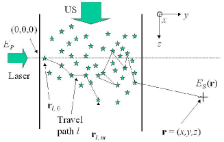
Figure 1: Light scattering along the travel path $l$, which involves scattering event located in $\textbf{r}_{l,m}$, where $m$ is the scattering event index.

Let us call $E_{P}$ and $E_{S}$ the fields coming into and out of the sample. Consider the point ($x,y$) located after the sample output interface. $E_{S}$ is a quasi monochromatic wave at the frequency $\omega_{0}$ of the incoming laser. Let’s introduce the complex field amplitude ${\underline{E}}_{P}$ and ${\underline{E}}_{S}$ defined as:

$$E_{P}(t)=\Re\left\{{\underline{E}}_{P}e^{j\omega_{0}t}\right\}$$ (1)

$$E_{S}(t)=\textbf{$\Re$}\left\{{\underline{E}}_{S}e^{j\omega_{0}t}\right\}$$ (2)

where $\Re$ is the real part operator. $E_{S}$ results from the sum (or the interference) of the field components $E_{S,l}$ scattered through the sample along many travel paths $l$ from input plane ($z=0$) to the detector. Moreover, as illustrated by Fig.1, each travel path $l$ can be decomposed in a succession of scattering events ($l,m$) located in $\textbf{r}_{l,m}$ where $m$ is the scattering events index.

$$E_{S}\left(t\right) = \sum_{l}E_{S,l}\left(t\right)$$

$$= \textbf{$\Re$}\left\{\sum_{l}~{}a~{}{\underline{E}}_{P}~{}e^{j\omega_{0}\left(t-{s_{l}}/{c}\right)}\right\}$$

where $l$ is the travel path index, and $s_{l}$ the corresponding effective travel path length. The length $s_{l}$ is the product of the travel path length by the medium refractive index $n$. To simplify the discussion we consider that the field amplitude $a$ is the same for all the travel paths. All travel paths have the same weight $a{\underline{E}}_{P}$, but different field phases: $e^{-j~{}\omega_{0}s_{l}/c}\equiv e^{-j~{}2\pi s_{l}/\lambda}$. Since the travel path lengthes are large with respect to the optical wavelength $\lambda$, the factor $e^{-j{2\pi s_{l}}/{\lambda}}$ is random. Summing over the travel paths, one gets a speckle outgoing field.

2.1.1 The ultrasonic field of pressure

Let us now apply a CW (Continuous Wave) ultrasonic (US) wave to the system by using an ultrasonic piezoelectric (PZT) device. The PZT transducer excitation voltage is:

$$U_{PZT}(t)=\textbf{$\Re$}\left\{{\underline{U}}_{PZT}\;e^{j\omega_{US}t}\right\}$$ (4)

where $\underline{U}_{PZT}$ is the complex amplitude of $U_{PZT}$. Like in experiments, we consider here linear conditions where the acoustic pressure $P_{US}$ is proportional to the excitation voltage. By this way, we get in any point r of the sample:

$$P_{US}(\textbf{r},t)=A(\textbf{r})\;{U}_{PZT}\left(t-{z}/{c_{US}}\right)$$ (5)

where $c_{US}$ is the sound velocity in the sample, and ${z}/{c_{US}}$ the time delay from the US emission point (the PZT) to the zone of coordinate $z$ that is considered. Let us introduce the US pressure complex amplitude ${\underline{P}}_{US}$:

$$P_{US}(\textbf{r},t) = \Re~{}\left\{{\underline{P}}_{US}(\textbf{r})~{}e^{j\omega_{US}t}\right\}$$ (6)

with

$${\underline{P}}_{US}(\textbf{r}) = A(\textbf{r})~{}{\underline{U}}_{PZT}~{}e^{{-j\omega_{US}z}/{c_{US}}}$$ (7)

The pressure $\underline{P}_{US}$ is periodic with respect to the US propagation axis, the period being $\lambda_{US}=2\pi{c_{US}}/{\omega_{US}}$.

2.1.2 The acousto optic modulation

Because of the US beam the scatterers vibrate. Moreover, the sample refractive index is modulated. These two effects yield a modulation of the length $s_{l}$ of the travel paths of the photons that are scattered by the medium (where $l$ is the travel path index) at the US frequency $\omega_{US}$:

$$s_{l}(t)=s_{l,0}-\Re\left\{\underline{\delta s}_{l}\;e^{j\omega_{US}~{}t}\right\}$$ (8)

where $\underline{\delta s}_{l}$ is the complex amplitude of the modulation of the travel path $l$. We get from Eq.2.1:

$$E_{S}\left(t\right) = \textbf{$\Re$}\sum_{l}~{}a~{}{\underline{E}}_{P}~{}e^{j~{}\omega_{0}\left(t-{s_{l,0}}/{c}\right)}~{}$$

$$\times\exp\left[j~{}\frac{\omega_{0}}{c}\Re\left\{\underline{\delta s}_{l}\;e^{j\omega_{US}~{}t}\right\}\right]$$

Let us introduce the complex amplitude $\underline{\delta s}_{l,m}$ of the $\textrm{m}^{th}$ scatterer contribution to the travel path modulation, whose modulus and phase are $\beta_{l,m}$ and $\phi_{l,m}$ respectively.

$$\underline{\delta s}_{l}=\sum_{m}\underline{\delta s}_{l,m}=\sum_{m}\beta_{l,m}e^{j\phi_{l,m}}$$ (10)

The sample outgoing field $E_{S}(t)$ is then modulated by the US at frequency $\omega_{US}$.

$$E_{S}(t) = a\;\Re\;\sum_{l}\;{\underline{E}}_{P}\;e^{j\;\omega_{0}\left(t-{s_{l,0}}/{c}\right)}~{}$$

$$\times\exp\left[j~{}\frac{\omega_{0}}{c}\sum_{m}\Re\left[~{}\underline{\delta s}_{l,m}e^{j\omega_{US}t}\right]\right]$$

2.1.3 The tagging of the scattered photons

In typical experiments, the vibration amplitude is much lower than the optical wavelength $\lambda=2\pi{c}/{\omega_{0}}$: for example, the vibration amplitude is 60 nm for 1 MPa acoustic pressure at $\omega_{US}=2$ MHz. We can then make the hypothesis of a weak acousto optic modulation:

$$\frac{\omega_{0}}{c}\sum_{m}\Re\left\{\underline{\delta s}_{l,m}e^{j\omega_{US}t}\right\}~{}\ll~{}1$$ (12)

We get in Eq.2.1.2:

$$\exp\left[j~{}\frac{\omega_{0}}{c}\sum_{m}\Re\left\{\underline{\delta s}_{l,m}e^{j\omega_{US}t}\right\}\right]\simeq$$ (13)

$$~{}~{}~{}~{}~{}~{}~{}~{}1+j~{}\frac{\omega_{0}}{c}\sum_{m}\Re\left\{\underline{\delta s}_{l,m}e^{j\omega_{US}t}\right\}$$

The field $E_{S}(t)$ diffused by the sample becomes:

$$E_{S}(t)=\Re\left\{\left[a\;\sum_{l}\;{\underline{E}}_{P}\;e^{j\omega_{0}\left(t-{s_{l,0}}/{c}\right)}\right]\right.$$

$$\left.\times\left[1+j~{}\frac{\omega_{0}}{c}\sum_{m}\Re\left\{\underline{\delta s}_{l,m}e^{j\omega_{US}t}\right\}\right]\right\}$$ (14)

The field $E_{S}(t)$ diffused by the sample is the sum of a main component $E_{S,\omega_{0}}(t)$, whose frequency is $\omega_{0}$, with the two sideband components $E_{S,\omega_{\pm 1}}(t)$, whose frequencies are $\omega_{\pm 1}=\omega_{O}\pm\omega_{US}$.

$$E_{S}(t) = E_{S,\omega_{0}}(t)+E_{S,\omega_{1}}(t)+E_{S,\omega_{-1}}(t)$$ (15)

Let us introduce ${\underline{E}}_{S,\omega_{0}}$ and ${\underline{E}}_{S,\omega_{\pm 1}}$, which are slow varying with time.

$$E_{S,\omega_{0}}(t) \equiv \Re~{}\left\{{\underline{E}}_{S,\omega_{0}}\exp(j\omega_{0}t)\right\}$$ (16)

$$E_{S,\omega_{\pm 1}}(t) \equiv \Re~{}\left\{{\underline{E}}_{S,\omega_{\pm 1}}\exp(j\omega_{\pm 1}t)\right\}$$

We get from Eq.2.1.3:

$$E_{S,\omega_{0}}(t)=\Re\left\{\;a\;\sum_{l}\;{\underline{E}}_{P}\;e^{j\;\omega_{0}\left(t-{s_{l,0}}/{c}\right)}\right\}$$ (17)

$$E_{S,\omega_{1}}(t)+E_{S,\omega_{-1}}(t)=\Re~{}\left\{a{\underline{E}}_{P}e^{j\omega_{0}t}\vphantom{\sum_{l,m}\left[j\frac{2\pi\beta_{l,m}}{\lambda}~{}e^{-j{2\pi s_{l,0}}/{\lambda}}\left[e^{j\phi_{l,m}}\;e^{~{}j\omega_{US}t}+c.c.\right]~{}\right]}\right.$$ (18)

$$\left.\times\sum_{l,m}\left[j\frac{2\pi\beta_{l,m}}{\lambda}~{}e^{-j{2\pi s_{l,0}}/{\lambda}}\left[e^{j\phi_{l,m}}\;e^{~{}j\omega_{US}t}+c.c.\right]~{}\right]\right\}$$

where $c.c.$ means the complex conjugate. We thus have for ${\underline{E}}_{S,\omega_{\pm 1}}$:

$${\underline{E}}_{S,\omega_{\pm 1}}(t) = a{\underline{E}}_{P}\sum_{l}$$

$$\left[j~{}e^{-j{2\pi s_{l,0}}/{\lambda}}\times\sum_{m}\left[\frac{2\pi\beta_{l,m}}{\lambda}e^{\pm j\phi_{l,m}}\right]\right]$$

Here, the main component $E_{S,\omega_{0}}$ does not depend on the travel path modulation (Eq.17), while the modulated components $E_{S,\omega_{\pm 1}}$ do. Moreover, whatever the modulation mechanism is: displacement of the scatterers or modulation of the refractive index, $\beta_{l,m}$ is directly related to the acoustic pressure $P_{US}\left(\textbf{r}_{l,m}\right)$ at the scatterer location $\textbf{r}_{l,m}$.

Note that the phases $\phi_{l,m}$ and $\phi_{l,m^{\prime}}$ of two scattering events $m$ and $m^{\prime}$ of the same path $l$ are partially correlated according to the position of the associated diffusers $\textbf{r}_{l,m}$ and $\textbf{r}_{l,m^{\prime}}$, and according to the physical effect at the origin of the modulation.

For the displacement of the scatterers, the phases $\phi_{l,m}$ is related to the projection $q_{z}$ of the scattering wave vector $\textbf{q}_{l,m}$ along the US propagation direction (i.e $z$) with $\textbf{q}_{l,m}=\textbf{k}^{\prime}_{l,m}-\textbf{k}_{l,m}$ (where $\textbf{k}_{l,m}$ and $\textbf{k}^{\prime}_{l,m}$ are the wave vectors of the photon before and after the scattering event $l,m$). The phases $\phi_{l,m}$ and $\phi_{l,m^{\prime}}$ are not correlated, since $q_{z}$ may change of sign from one scattering event ($l,m$) to the next ($l,m+1$) within the same path $l$.

For the modulation of the refractive index, $\phi_{l,m}$ is mainly related to the US phase. In a typical experiment the scattering length $l_{s}$ is about $0.1$ mm, while the US wavelength $\lambda_{US}$ is about 1 mm (0.75 mm for $\omega_{US}=2$ MHz). This means that $\phi_{l,m}$ and $\phi_{l,m^{\prime}}$ are correlated, if the scattering events ($l,m$) and ($l,m^{\prime}$) are close together ($|m-m^{\prime}|<$a few units), and uncorrelated if not.

This partial coherence allows us to use the acousto-optical modulation in scattering media. However, all the scatterers $\textbf{r}_{l,m}$ in the acoustic column contribute to the tagged photons field ${\underline{E}}_{S,\omega_{\pm 1}}(t)$. Thus on the acoustic column, the information is not localized. So it is necessary to use a complementary technique in order to obtain an axial $z$ resolution.

2.2 The axial resolution along $z$

To obtain an axial resolution along $z$, Lesaffre et al. [30] have used Acousto Optic Cohérent Tomography (AOCT). This technique is based on the control of the acoustic and optical coherence lengths using a random phase modulation on the acoustic and optical arms.

2.2.1 The AOCT random modulation of the optical and acoustical field phases.

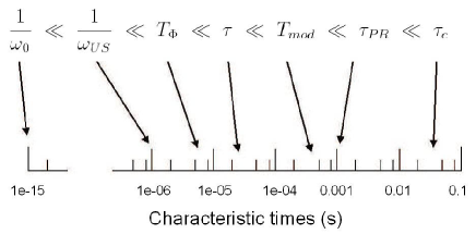
Figure 2: Order of magnitude of the various times. $1/\omega_{0}$: optical period; $1/\omega_{US}$: acoustic period; $T_{\Phi}$: acousto-optical correlation time; $\tau$: time averaging characteristic time; $T_{mod}$: characteristic time of the modulation $H(t)$; $\tau_{PR}$: photorefractive time; $\tau_{c}$: Lock-in integration time.

The incoming optical field and the PZT excitation voltage are now:

$$E^{\prime}_{P}(t)=\textbf{$\Re$}~{}\left\{{\underline{E}}_{P}e^{j(\omega_{0}t+\psi_{P}(t)~{})}\right\}$$ (20)

$$U^{\prime}_{PZT}(t)=\Re~{}\left\{{\underline{U}}_{PZT}~{}e^{j(\omega_{US}t-\psi_{US}(t)~{})}\right\}$$ (21)

where $\psi_{P}$ et $\psi_{US}$ are random phase modulations applied to the optical incoming beam $E^{\prime}_{P}$ and to the PZT that generates the US beam. Since we consider the effect of a random phase modulation, fields are noted $E^{\prime}_{P}$, $E^{\prime}_{S}$ . The random phases $\psi_{P}(t)$ and $\psi_{US}(t)$ are supposed to be fully correlated as follow:

$$\psi_{P}\left(t\right)=\psi_{US}\left(t-z_{0}/c_{US}\right)$$ (22)

where $z_{0}/c_{US}=\theta$ is a fixed temporal delay which determines the $z$ selected zone $z\simeq z_{0}$.

To simplify the discussion we will consider here, like in [30], that the US phase $\psi_{US}$ is randomly drawn every $T_{\Phi}$ to be 0 or $\pi$ with equal probability. The optical phase $\psi_{P}$ follows the same random phase law than $\psi_{US}$, but the phase is dealyed in time by $z_{0}/c_{US}$. The incoming complex field is:

$${\underline{E}^{\prime}}_{P}(t)={\underline{E}}_{P}e^{j\psi_{P}(t)~{}}$$ (23)

and the US excitation (${\underline{U}}^{\prime}_{PZT}$), and US pressure (${\underline{P}}^{\prime}_{US}$) complex amplitudes are:

$${\underline{U}}^{\prime}_{PZT}(t) = ~{}{\underline{U}}_{PZT}~{}e^{j\psi_{US}(t)}$$ (24)

$${\underline{P}}^{\prime}_{US}(\textbf{r},t) = A(\textbf{r})~{}{\underline{U}}_{PZT}\;e^{{j\omega_{US}z}t/{c_{US}}}\;e^{~{}j\psi_{US}(t-{z}/{c_{US}})}$$

2.2.2 The "tagged photons" field.

By making the calculations leading to Eq.2.1.3 with the random phases $\psi_{P}$ and $\psi_{US}$, we get the tagged photons complex amplitude ${\underline{E}}^{\prime}_{S,\omega_{\pm 1}}$:

$${\underline{E}}^{\prime}_{S,\omega_{\pm 1}}(t)=a{\underline{E}}_{P}~{}\sum_{l}\left[j~{}e^{-j{2\pi s_{l,0}}/{\lambda}}\vphantom{\frac{2\pi\beta_{l,m}}{\lambda}\sum_{m}}\right.$$ (25)

$$\left.\times\sum_{m}\frac{2\pi\beta_{l,m}}{\lambda}e^{~{}\pm j\phi_{l,m}}~{}e^{~{}\pm j\psi_{l,m}(t)}~{}\right]$$

where the phase $\psi_{l,m}$, which depends on time $t$, and on location $z_{l,m}$ of the $m^{th}$ scatterer along the axis $z$, is defined by:

$$\psi{}_{l,m}(t)=\psi_{P}(t)+\psi_{US}\left(t-{z_{l,m}}/{c_{US}}\right).$$ (26)

Because of the random phase jumps, which occur every $T_{\phi}$, the complex field ${\underline{E}}^{\prime}_{S,\omega_{\pm 1}}(t)$ varies with a characteristic time $T_{\phi}$, while, in absence of random modulation, the field ${\underline{E}}_{S,\omega_{\pm 1}}$ does not depend on time. In the following, we will detect the field ${\underline{E}}^{\prime}_{S,\omega_{\pm 1}}(t)$ by photorefractive effect on a crystal.

We must notice that all the photorefractive detection ${\underline{E}}^{\prime}_{S,\omega_{\pm 1}}(t)$ processes occur on times much larger than $T_{\phi}$.

• The writing of photorefractive signal on the crystal occurs in a time $\tau_{PR}\gg T_{\phi}$.

• To get a modulated signal for the Lock-In amplifier, the phase of the US will be modulated at a frequency $\omega_{mod}=1/T_{mod}$ with $T_{mod}\gg T_{\phi}$.

• The extraction of the modulated signal modulated at $\omega_{mod}$ will be made via Lock-In with an integration time $\tau_{c}\gg T_{\phi}$.

So one can replace in the following the field ${\underline{E}^{\prime}}_{S,\omega_{\pm 1}}(t)$ by its temporal average $\langle{\underline{E}^{\prime}}_{,\omega_{\pm 1}}(t)\rangle_{\tau}$ over the characteristic time $\tau$ chosen such as (see Fig.2):

$$T_{\phi}\ll\tau\ll\tau_{PR},\;T_{mod},\;\tau_{c}$$ (27)

Thus we eliminate the fast varying components of ${\underline{E}}^{\prime}_{S,\omega_{\pm 1}}(t)$ which anyway will have no effect on the final signal. To be complete let’s define here the temporal average operator $\langle\;\rangle_{\tau}$ :

$$\langle....\rangle_{\tau}\equiv\frac{1}{\tau}\int_{t^{\prime}=t-\tau/2}^{t^{\prime}=t+\tau/2}(....)dt^{\prime}$$ (28)

The temporal average of the tagged photon field over the characteristic time $\tau$ is then:

$$\langle{\underline{E}^{\prime}}_{S,\omega_{\pm 1}}(t)\rangle_{\tau}=a{\underline{E}}_{P}~{}\sum_{l}\left[j~{}e^{-j{2\pi s_{l,0}}/{\lambda}}\phantom{\sum_{m}\frac{2\pi\beta_{l,m}}{\lambda}}\right.$$

$$~{}~{}~{}~{}\left.\times\sum_{m}\left(\frac{2\pi\beta_{l,m}}{\lambda}e^{\pm j\phi_{l,m}}\times\langle e^{\pm j\psi_{l,m}(t)}\rangle_{\tau}\right)\right]$$ (29)

As we can see on Eq.2.2.2, $\psi_{l,m}$ acts on the temporal average $\langle{\underline{E}^{\prime}}_{S,\omega_{\pm 1}}(t)\rangle_{\tau}$ only through $\langle e^{\pm j\psi_{l,m}(t)}\rangle_{\tau}$, which depends only on the location along $z$ of the scatterer of indexes $l,m$, i.e. on $z_{l,m}$. From Eq.22 and Eq.26, we have

$$\psi_{l,m}(t) \simeq 0$$

$$\langle e^{~{}\pm j\psi_{l,m}(t)}\rangle_{\tau} \simeq 1$$ (30)

$$\psi_{l,m}(t) \simeq 0,\pi~{}~{}~{}\textrm{randomly}$$

$$\langle e^{\pm j\psi_{l,m}(t)}\rangle_{\tau} \simeq 0$$ (31)

for the scatterer $l,m$ located in (Eq.2.2.2) and out (Eq.2.2.2) the selected zone $z\simeq z_{0}$ respectively.

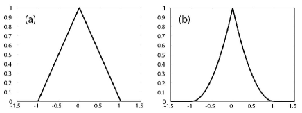
Figure 3: Plot of correlation function $\underline{g}_{1}(\theta)$ (a), and its square $|\underline{g}_{1}(\theta)|^{2}$ (b). The horizontal axis Units is either $\theta/T_{\Phi}$ (for time correlation), or $(z-z_{0})/\Delta z$ with $\Delta z=c_{US}~{}T_{\Phi}$ (for $z$ resolution).

To characterize this $z$ selection mechanism in a more quantitative way, let us define the time correlation function:

$$\underline{g}_{1}(\theta) = \frac{\langle{\underline{E}}^{\prime}_{P}(t){\underline{E}}{}_{P}^{\prime*}(t+\theta)\rangle_{\tau}}{\langle\left|{\underline{E}}^{\prime}_{P}(t)\right|^{2}\rangle_{\tau}}$$

$$= \left\langle e^{j\psi_{P}(t)}e^{-j\psi_{P}(t+\theta)}\right\rangle_{\tau}$$

$$= \left\langle e^{j\psi_{US}(t)}e^{-j\psi_{US}(t+\theta)}\right\rangle_{\tau}$$

$$= \frac{\langle{{\underline{U}}^{\prime}_{US}(t){\underline{U}}{}_{US}^{\prime*}(t+\theta)}\rangle_{\tau}}{\langle{\left|{\underline{U}}^{\prime}_{US}(t)\right|^{2}}\rangle_{\tau}}$$

In the case of $0,\pi$ random phase jumps considered here, $\underline{g}_{1}(\theta)$ is a triangular function that corresponds to the convolution of two rectangles of width $T_{Phi}$. The correlation function $\underline{g}_{1}(\theta)$ is plotted on Fig.3 (a).

The field $\langle{\underline{E}^{\prime}}_{S,\omega_{\pm 1}}\rangle$ can be expressed as a function of $\underline{g}_{1}$:

$$\langle{\underline{E}^{\prime}}_{S,\omega_{\pm 1}}(t)\rangle_{\tau}=a{\underline{E}}_{P}\sum_{l}\left[j~{}e^{-j{2\pi s_{l,0}}/{\lambda}}\vphantom{\sum_{m}}\right.$$ (33)

$$~{}~{}~{}~{}\left.\times\sum_{m}\left[\underline{g}_{1}\left(\frac{z_{l,m}-z_{0}}{c_{US}}\right)~{}\frac{2\pi\beta_{l,m}}{\lambda}e^{\pm j\phi_{l,m}}\right]\right]$$

Let us note here that the second member of Eq. 33 does not depend on time. It means that, when we apply the random modulations of phase, the field ${\underline{E}^{\prime}}_{S,\omega_{\pm 1}}(t)$ reaches, after a brief transitory regime, a stationary regime in which the slow field components do not depend on time any more.

Furthermore, the results of the calculations do not depend on $\tau$ as soon as the condition $T_{\phi}\ll\tau\ll(\tau_{PR},\;T_{mod},\;\tau_{c})$ of Eq.27 is fulfilled. So one should write: $\langle{\underline{E}^{\prime}}_{S,\omega_{\pm 1}}(t)\rangle_{\tau}\equiv\langle{\underline{E}^{\prime}}_{S,\omega_{\pm 1}}\rangle$.

2.3 The photorefractive detection of the tagged photons

We will now consider the photorefractive detection of the tagged photons in order to quantify the $z$ selection process for the photorefractive detected signal (and not just for the tagged field ${\underline{E}^{\prime}}_{S,\omega_{\pm 1}}$ itself). The calculations we will make are similar to the ones made by Gross at al. [22], but in a slightly different context.

2.3.1 The detection principle

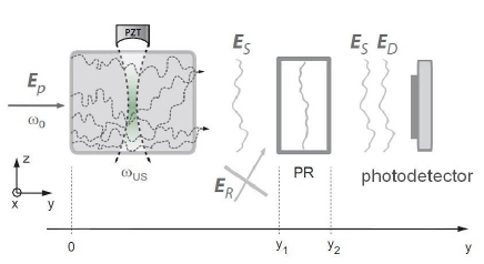
Figure 4: Principle of the photorefractive detection.

The principle of the photorefractive detection is illustrated on Fig.4. The signal $E_{S}$, the wave front of which is distorted, is collected in a photorefractive crystal. A reference beam $E_{R}$, considered as plane wave, which is also called pump beam, interferes with it within the crystal. By photorefractive effect, the interferogram grooves a hologram corresponding to a weak modulation $\delta n(\textbf{r})$ of the local refractive index within the volume of the crystal. This effect having a finite response time $\tau_{PR}$, only the static component of the interferogram contributes to the recording of the hologram.

To simplify the analysis, we will consider the detection of tagged photons of the $+1$ sideband at $\omega_{1}=\omega_{0}+\omega_{US}$. So we will shift the beam reference frequency by $\omega_{US}=\omega_{1}-\omega_{0}$ in order to perform the photorefractive detection at frequency $\omega_{1}$. Let us introduce the complex amplitude ${\underline{E}}_{R,\omega_{1}}$ of the reference field.

$$E_{R}(t)=\Re~{}\left[{\underline{E}}_{R,\omega_{1}}e^{j\omega_{1}t}\right]$$ (34)

The photorefractive effect selects, in the signal field $E^{\prime}_{S}=E^{\prime}_{S,\omega_{0}}+E^{\prime}_{S,\omega_{1}}+E^{\prime}_{S,\omega_{-1}}$, the field component $E^{\prime}_{S,\omega_{1}}$. The reference beam is then diffracted by the holographic grating grooved within the crystal yielding the field $E^{\prime}_{D}$, whose wavefront is the same for $E^{\prime}_{S,\omega_{1}}$. At the exit of the crystal, one gets then both the transmitted signal beam $E_{S}^{\prime}$, and the beam diffracted by the crystal, which will be noted $E^{\prime}_{D}$.

2.3.2 The reference field diffracted by the crystal $E^{\prime}_{D}$

Let us introduce the complex amplitude of the diffracted field defined by

$$E^{\prime}_{D}(t)=\Re~{}\left[{\underline{E}}^{\prime}_{D,\omega_{1}}(t)e^{j\omega_{1}t}\right]$$ (35)

Let us call $y=y_{1}$ and $y=y_{2}$ the crystal entrance and exit planes respectively, and $t=0$ the origin of time, when no photorefractive hologram is recorded. Let us consider that the reference field ${\underline{E}}_{R}$ is constant.Within the crystal, the signal field ${\underline{E}}^{\prime}_{S,\omega_{1}}(y_{1}<y<y_{2},\,t)$ can be written as a function of the entrance field ${\underline{E}}^{\prime}_{S,\omega_{1}}(y_{1},t)$ [32, 33]

$${\underline{E}}^{\prime}_{S,\omega_{1}}(y,t)=e^{{-\alpha(y-y_{1})}/{2}}$$ (36)

$$~{}~{}~{}\times\left[~{}{\underline{E}}^{\prime}_{S,\omega_{1}}(y_{1},t)+\int_{0}^{t}dt^{\prime}{\underline{E}}^{\prime}_{S,\omega_{1}}(y_{1},t^{\prime})G(y,t-t^{\prime})\right]$$

where, under conditions of weak recording efficiency and weak absorption, the transfer function $G(y,t)$ can be written as [34]

$$G(y,t)=\frac{\gamma(y-y_{1})}{\tau_{PR}}e^{-\frac{t}{\tau_{PR}}}$$ (37)

Here, $\tau_{PR}$ is the photorefractive response time and $\gamma$ the photorefractive gain. Equation 36 is established for two plane waves, but it can be generalized to distorted wavefront by decomposing the wavefront in plane waves. Several approximations are made to establish this equation: (i) the reference beam is a monochromatic wave with constant frequency $\omega_{1}$ (i.e. it is not temporarily modulated), (ii) it is not perturbed by the recording of the hologram although it can be attenuated by the crystal, and (iii) its power is larger than the signal beam one.

In the AOCT experiment [30], the tagged photon signal is modulated at a frequency $\omega_{mod}$ of some kHz, and Lock-in detection is performed. So we are interested in the low-frequency evolution of $\underline{E}^{\prime}_{S,\omega_{1}}$. So we can replace the $t^{\prime}=0$ lower limit of the integral $\int dt^{\prime}$ of Eq. 36 by $t^{\prime}=-\infty$, by neglecting the transient components. By making the transformation $t^{\prime}\rightarrow(t-t^{\prime})$, in the integral $\int dt^{\prime}$ of Eq.2.1, we obtain:

$$\underline{E}^{\prime}_{S,\omega_{1}}(y,t)=e^{{-\alpha(y-y_{1})}/{2}}$$ (38)

$$\times\left[~{}{\underline{E}}^{\prime}_{S,\omega_{1}}(y_{1},t)+\int_{0}^{\infty}{dt^{\prime}}~{}{\underline{E}}^{\prime}_{S,\omega_{1}}(y_{1},t-t^{\prime})~{}G(y,t^{\prime})~{}\right]$$

We can notice that the hologram is written with delayed time $t-t^{\prime}$ with a delay $t^{\prime}$ varying from zero to some $\tau_{PR}$. Also let us note that the first term of Eq. 38 corresponds to the signal wavefront that is transmitted by the crystal. Let us call $E^{\prime}_{T}$ its field and $\underline{E}^{\prime}_{T}$ its complex amplitude (the index $T$ means here transmitted). The second term corresponds to the reference field that is diffracted by the crystal we will note $E^{\prime}_{D}$ (where the index $D$ means diffracted), and $\underline{E}^{\prime}_{D}$ for the complex amplitude. We can write:

$$E^{\prime}_{S}(y,t) = E^{\prime}_{T}(y,t)+E^{\prime}_{D}(y,t)$$ (39)

$$E^{\prime}_{T}(y,t) = E^{\prime}_{T,\omega_{-1}}(y,t)+E^{\prime}_{T,\omega_{0}}(y,t)+E^{\prime}_{T,\omega_{+1}}(y,t)$$

$$E^{\prime}_{D}(y,t) = E^{\prime}_{D,\omega_{+1}}(y,t)$$

$$\underline{E}^{\prime}_{S,\omega_{1}}(y,t) = \underline{E}^{\prime}_{T,\omega_{1}}(y,t)+\underline{E}^{\prime}_{D,\omega_{1}}(y,t)$$ (40)

$$\underline{E}^{\prime}_{T,\omega_{1}}(y,t) = ~{}e^{-\alpha(y-y_{1})/2}{\underline{E}^{\prime}}_{S,\omega_{1}}(y_{1},t)$$

$$\underline{E}^{\prime}_{D,\omega_{1}}(y,t) = e^{-\alpha(y-y_{1})/2}$$

$$~{}~{}~{}\times\int_{0}^{\infty}{dt^{\prime}}{\underline{E}^{\prime}}_{S,\omega_{1}}(y_{1},t-t^{\prime})G(y,t^{\prime})$$

Note that since the photorefractive effect selects the field components of frequency $\omega_{1}$, the diffracted field $E^{\prime}_{D}$ exhibit in Eq.39 a single frequency component $E^{\prime}_{D,\omega_{+1}}$.

2.4 The acousto optic signal detected by a large area photodiode

We consider that the signal is detected by a photodiode of large area located near the cristal exit plane $y=y_{2}$. The photodiode signal $S_{PD}$ is equal to the integral of $|\underline{E}^{\prime}_{S}|^{2}$ over its area. We get from Eq.39.

$$S_{PD}(t)=c.c.+$$ (41)

$$~{}~{}\int dx\int dz~{}~{}\left|{\underline{E}^{\prime}_{S}}(x,y_{2},z,t)\right|^{2}$$

$$S_{PD}(t)=c.c.+$$ (42)

$$~{}~{}\int dx\int dz~{}\left\{~{}\left|{\underline{E}^{\prime}_{T}}(x,y_{2},z,t)\right|^{2}\right.$$

$$~{}~{}\left.\qquad+~{}\left|{\underline{E}^{\prime}_{D}}(x,y_{2},z,t)\right|^{2}\right.$$

$$~{}~{}\left.\qquad+~{}\left(~{}\underline{E}^{\prime}_{T}(x,y_{2},z,t)~{}{\underline{E}{}_{D}^{\prime*}}(x,y_{2},z,t)\right)\right\}$$

Because the acousto-optical interaction does not modify the total number of photons, i.e. tagged + untagged photons, the term $|\underline{E}^{\prime}_{T}|^{2}$ in Eq.42 does not depend on the acoustic modulation. Furthermore, because the gain is supposed to be low, i.e. $\eta_{PR}=\gamma(y_{2}-y_{1})<1$, the term $|\underline{E}^{\prime}_{D}|^{2}$ can be neglected in front of the crossed term $\underline{E}^{\prime}_{T}~{}{\underline{E}^{\prime}_{D}}^{*}$. Therefore we can only consider the crossed term, which is the product of the diffracted field $E_{D}^{\prime}$, which builts up with the characteristic time $\tau_{PR}$, and the transmitted field $E^{\prime}_{T}$, which can vary quickly. The photodiode modulated signal $S^{\prime}_{PD}$ is thus:

$$S^{\prime}_{PD}(t)=c.c.+$$ (43)

$$\int dx\int dz~{}\underline{E}^{\prime}_{T,\omega_{1}}(x,y_{2},z,t){\underline{E}{}_{D,\omega_{1}}^{\prime*}}(x,y_{2},z,t)$$

From Eq.40, we get

$$S^{\prime}_{PD}(t)=c.c.+$$ (44)

$$e^{-\alpha(y_{2}-y_{1})}\;\int dx\int dz\;{\underline{E}}^{\prime}_{S,\omega_{1}}(x,y_{1},z,t)$$

$$\quad\times\int_{0}^{\infty}{dt^{\prime}}~{}{\underline{E}_{S,\omega_{1}}^{\prime*}}(x,y_{1},z,t-t^{\prime})~{}G^{*}(y_{2},t^{\prime})$$

To keep a certain universality, we write $G^{*}$ although $G$ is supposed to be real. We can then develop ${\underline{E}}^{\prime}_{S,\omega_{1}}$ by summing up all the paths (index $l$) and scattering events (index $m$) contributions by using Eq.33. Averaging over a time $\tau$, we get:

$$\langle S^{\prime}_{PD}(t)\rangle_{\tau}=c.c.+e^{-\alpha(y_{2}-y_{1})}|a\underline{E}_{p}|^{2}\;\int dx\int dz\;$$

$$\left[\sum_{l}je^{-j{2\pi s_{l,0}}/{\lambda}}\times\sum_{m}\frac{2\pi\beta_{l,m}}{\lambda}~{}\underline{g}_{1}\left(\frac{z_{0}-z_{l,m}}{v_{US}}\right)e^{j\phi_{l,m}}\right]$$

$$\times\left[\int_{0}^{\infty}dt^{\prime}~{}~{}G^{\ast}(y_{2},t^{\prime})\times\left(\sum_{l^{\prime}}-j~{}e^{{2j\pi s_{l^{\prime},0}}/{\lambda}}\right.\right.$$

$$\quad\quad\left.\left.\times\sum_{m^{\prime}}\frac{2\pi\beta_{l^{\prime},m^{\prime}}}{\lambda}\;\underline{g}_{1}^{*}\left(\frac{z_{0}-z_{l^{\prime},m^{\prime}}}{v_{US}}\right)~{}e^{-j\phi_{l^{\prime},m^{\prime}}}\right)\right]$$

The equation 2.4 illustrates the complexity of the calculation of the signal. It involves a double summation over the optical paths ( i.e. $\sum_{l,l^{\prime}}$), a double summation over the scattering events (i.e. $\sum_{m,m^{\prime}}$), a spatial integral over the photodiode area (i.e. $\int\int dx~{}dz$), and a temporal integral over the delay $t^{\prime}$ (i.e. $\int dt^{\prime}$).

To simplify this equation, let us consider first the integral over the photodiode area $\int\int dx\>dz$. Every point ($x,z$) of the photodiode selects paths $l$ and $l^{\prime}$, which finishes in ($x,z$). For the corresponding paths, the phase factor $e^{-j{2\pi\;s_{l,0}}/{\lambda}}$ is totally random from a route to the next one. So we can limit the summation over $l$ and $l^{\prime}$ to the terms $l=l^{\prime}$. The equation 2.4 becomes then:

$$\langle S^{\prime}_{PD}(t)\rangle_{\tau}=c.c.+e^{-\alpha(y_{2}-y_{1})}\left|\frac{2\pi a\underline{E}_{p}}{\lambda}\right|^{2}\;\int dx\int dz$$

$$~{}~{}\times\sum_{l}\sum_{m}\left[\beta_{l,m}\;\underline{g}_{1}\left(\frac{z_{0}-z_{l,m}}{c_{US}}\right)\right.\int_{0}^{\infty}dt^{\prime}G^{\ast}(y_{2},t^{\prime})$$

$$~{}~{}\left.\times\sum_{m^{\prime}}\beta_{l,m^{\prime}}\;\underline{g}_{1}^{*}\left(\frac{z_{0}-z_{l,m^{\prime}}}{c_{US}}\right)e^{j(\phi_{l,m}-\phi_{l,m^{\prime}})}\right]$$ (46)

To simplify this equation further, it is necessary to study the mutual coherence of the phases $\phi_{l,m}$ and $\phi_{l,m^{\prime}}$ that corresponds to two different scattering events $m$ and $m^{\prime}$ of the same path $l$. According to the position of the scatterers, and according to the acousto-optical modulation mechanism, these phases are correlated or not. Nevertheless, when the two events ($m$ and $m^{\prime}$) occur in two $z$ coordinates $z_{l,m}$ and $z_{l,m^{\prime}}$ separated by more than an acoustic wavelength $\lambda_{US}$ (i.e. $|z_{l,m^{\prime}}-z_{l,m}|>\lambda_{US}$), the phases $\phi_{l,m}$ and $\phi_{l,m^{\prime}}$ are weakly correlated. We can then write:

$$\langle S^{\prime}_{PD}(t)\rangle_{\tau}=c.c.+$$ (47)

$$e^{-\alpha(y_{2}-y_{1})}\left|\frac{2\pi a\underline{E}_{p}}{\lambda}\right|^{2}\intop_{0}^{\infty}dt^{\prime}G^{\ast}(y_{2},t^{\prime})\int dx\int dz$$

$$\sum_{l}\sum_{m}\sum_{m^{\prime}~{}\textrm{with}~{}\mid z_{l,m}-z_{l,m^{\prime}}\mid<\lambda_{US}}\left[\beta_{l,m}\beta_{l,m^{\prime}}\vphantom{\underline{g}_{1}^{*}\left(\frac{z_{0}-z_{l,m^{\prime}}}{c_{US}}\right)}\right.$$

$$\left.e^{j\left(\phi_{l,m}-\phi_{l,m^{\prime}}\right)}\underline{g}_{1}\left(\frac{z_{0}-z_{l,m}}{c_{US}}\right)\>\underline{g}_{1}^{*}\left(\frac{z_{0}-z_{l,m^{\prime}}}{c_{US}}\right)\right]$$

Since the magnitude of the acoustic pressure vary weakly over $\lambda_{US}$, we have $\beta_{l,m}\simeq\beta_{l,m^{\prime}}$ for $z_{l,m}-z_{l,m^{\prime}}<\lambda_{US}$. Moreover, the random modulation of phases is chosen in such a way that the characteristic length $T_{\phi}~{}c_{US}$ is larger than the acoustic wavelength $\lambda_{US}$ (i.e. $T_{\phi}~{}c_{US}>\lambda_{US}$. This implies that $\underline{g}_{1}\left((z_{0}-z_{l,m})/{c_{US}}\right)\simeq\underline{g}_{1}\left((z_{0}-z_{l,m^{\prime}})/{c_{US}}\right)$ for $z_{l,m}-z_{l,m^{\prime}}<\lambda_{US}$. Therefore we obtain:

$$\langle S^{\prime}_{PD}(t)\rangle_{\tau}=c.c.$$ (48)

$$+e^{-\alpha(y_{2}-y_{1})}\left|\frac{2\pi a\underline{E}_{p}}{\lambda}\right|^{2}\intop_{0}^{\infty}dt^{\prime}G^{\ast}(y_{2},t^{\prime})\int dx\int dz$$

$$\sum_{l}\sum_{m}\beta_{l,m}^{2}\;\left|\underline{g}_{1}\left(\frac{z_{0}-z_{l,m}}{c_{US}}\right)\right|^{2}$$

$$\quad\quad\times\sum_{m^{\prime}~{}\textrm{with}~{}\mid z_{l,m}-z_{l,m^{\prime}}\mid<\lambda_{US}}e^{j\left(\phi_{l,m}-\phi_{l,m^{\prime}}\right)}$$

Here, the term $\left|\underline{g}_{1}\left({z_{0}-z_{l,m}}/{c_{US}}\right)\right|^{2}$ selects the zone of imaging.

The $z$ resolution one can expect is roughly equal to the half-width of $\underline{g}_{1}(z)$, i.e. to $0.5\times c_{US}T_{\Phi}$ (see Fig.3). The expected resolution is thus about 7.5 mm for $T_{\Phi}=10$ $\mu$s (20 US periods at $\omega_{US}=2$ MHz), and 1.1 mm for $T_{\Phi}=1.5$ $\mu$s (3 US periods at $\omega_{US}=2$ MHz). The AOCT published experimental results [30] correspond to $T_{\Phi}\simeq 2$ $\mu$s. To improve the $z$ resolution, one must thus decrease $T_{\Phi}$. The acousto optic signal decreases accordingly, since it is proportional to $T_{\Phi}$: the scattering events that contribute to the signal must be within the $\underline{g}_{1}(z)$ selected region.

2.5 The Lock-in detection of the acousto optical signal

2.5.1 The modulation of the signal at $\omega_{mod}$

Note that $\langle S_{PD}(t)\rangle_{\tau}$ given by Eq.48 is invariant with time. So the tagged photons photorefractive signal $S_{PD}$ is a CW component, which adds to the total flow of transmitted light. To detect $S_{PD}$ more efficiently with a Lock-in, AOCT adds an extra modulation of the ultrasonic wave. Like in the AOCT experiment [30], we will consider here an asymmetric $0$ to $\pi$ phase modulation $H_{U.S.}(t)$ at frequency $\omega_{mod}=2\pi/T_{mod}\sim$ 3 kHz, with duty cycle $0<r<1$:

$$H_{US}(t) = +1\quad\quad\textrm{pour}\quad\quad 0\leq t/T_{mod}\leq r$$ (49)

$$H_{US}(t) = -1\quad\quad\textrm{pour}\quad\quad r<t/T_{mod}\leq 1$$

We consider that the modulation period $T_{mod}$ is very large compared to the correlation time $T_{\phi}$, but smaller than the photorefractive time $\tau_{PR}$, i.e. $({2\pi}/{\omega_{US}})<T_{\phi}\ll T_{mod}<\tau_{PR}$. In practice, we typically use $T_{mod}\sim 100\mu$s (see Fig.2). The modulation is applied according

$$\underline{U}^{\prime}_{PZT}(t)\rightarrow\underline{U}^{\prime\prime}_{PZT}(t)=~{}H_{US}(t)~{}\underline{U}^{\prime}_{PZT}(t)$$ (50)

The US signal is denoted $\underline{U}^{\prime\prime}_{PZT}(t)$, and the fields are denoted $E^{\prime\prime}_{P}$, $E^{\prime\prime}_{S}$ and so on. The complex amplitude of the tagged photon field is now

$$\underline{E}^{\prime}_{S,\omega_{1}}(t)\rightarrow\underline{E}^{\prime\prime}_{S,\omega_{1}}(t)=~{}H(t)~{}\underline{E}^{\prime}_{S,\omega_{1}}(t)$$ (51)

where $H(t)=H_{US}(t-z_{0}/c_{US})$. Similarly with Eq.40, the diffracted complex amplitude becomes

$$\underline{E}^{\prime\prime}_{D,\omega_{1}}(y,t) = e^{-\alpha(y-y_{1})/2}\int_{0}^{\infty}{dt^{\prime}}\left[H(t-t^{\prime})\right.$$ (52)

$$\left.\times{\underline{E}^{\prime}}_{S,\omega_{1}}(y_{1},t-t^{\prime})~{}G(y,t^{\prime})\right]$$

2.5.2 The modulated acousto-optical signal

The signal from the photodiode given by equation 44 becomes

$$S^{\prime\prime}_{PD}(t)=c.c.$$ (53)

$$\vphantom{\int dx}+~{}e^{-\alpha(y_{2}-y_{1})}\;\int dx\int dz\left[H(t)\vphantom{\int dx}{\underline{E}}^{\prime}_{S,\omega_{1}}(x,y_{2},z,t)\right.$$

$$\left.\int_{0}^{\infty}{dt^{\prime}}~{}H(t-t^{\prime})\;{\underline{E}^{\prime*}{}_{S,\omega_{1}}}(x,y_{2},z,t-t^{\prime})~{}G^{*}(y_{2},t^{\prime})\right]$$

By making the calculation leading to Eq. 48 from to Eq. 44 with the additional modulation $H_{US}$, we get.

$$\langle S^{\prime\prime}_{PD}(t)\rangle_{\tau}=c.c.+$$ (54)

$$e^{-\alpha(y_{2}-y_{1})}\left|\frac{2\pi a\underline{E}_{p}}{\lambda}\right|^{2}H\left(t\right)\intop_{0}^{\infty}dt^{\prime}H\left(t-t^{\prime}\right)G^{\ast}(y_{2},t^{\prime})$$

$$\times\int dx\int dz\sum_{l}\sum_{m}\left[\beta_{l,m}^{2}\;\left|\underline{g}_{1}\left(\frac{z_{0}-z_{l,m}}{c_{US}}\right)\right|^{2}\right.$$

$$\left.\times\sum_{m^{\prime}/\mid z_{l,m}-z_{l,m^{\prime}}\mid<\lambda_{US}}e^{j\left(\phi_{l,m}-\phi_{l,m^{\prime}}\right)}\right]$$

Since we have consider $T_{mod}<\tau_{PR}$, the integration over $t^{\prime}$ can be simplified, and we obtain from Eq.37.

$$\int_{0}^{\infty}dt^{\prime}H(t-t^{\prime})\;G^{\ast}(y_{2},t^{\prime})=~{}~{}~{}~{}~{}~{}~{}~{}~{}~{}~{}~{}~{}~{}~{}~{}~{}~{}~{}~{}~{}~{}~{}~{}~{}$$ (55)

$$~{}~{}~{}~{}\left[\frac{1}{T_{PR}}\int_{0}^{T_{PR}}dt^{\prime}H(t-t^{\prime})\right]\times\left[\int_{0}^{\infty}dt^{\prime}G^{\ast}(y_{2},t^{\prime})\right]$$

$$~{}~{}~{}~{}~{}~{}~{}~{}~{}~{}~{}~{}~{}~{}~{}~{}~{}~{}~{}~{}~{}~{}~{}~{}~{}~{}~{}~{}~{}~{}~{}~{}~{}~{}~{}~{}~{}=(1-2r)\;\gamma(y_{2}-y_{1})$$

This means that for a modulation $H(t)$ faster than $\tau_{PR}$, the photorefractive recorded hologram is proportional to the average $\langle H(t)\rangle_{\tau_{PR}}$. The asymmetric nature of the modulation $H\left(t\right)$ yields non-zero photorefractive grating. The modulated component of the signal on a large area photodiode thus becomes.

$$\langle S^{\prime\prime}_{PD}(t)\rangle_{\tau}\simeq c.c+$$ (56)

$$e^{-\alpha(y_{2}-y_{1})}\left|\frac{2\pi a\underline{E}_{p}}{\lambda}\right|^{2}H\left(t\right)(1-2r)\;\gamma(y_{2}-y_{1})$$

$$\times\int dx\int dz\sum_{l}\sum_{m}\beta_{l,m}^{2}\left|\underline{g}_{1}\left(\frac{z_{0}-z_{l,m}}{c_{US}}\right)\right|^{2}$$

$$\times\sum_{m^{\prime}/\mid z_{l,m}-z_{l,m^{\prime}}\mid<\lambda_{US}}e^{j\left(\phi_{l,m}-\phi_{l,m^{\prime}}\right)}$$

By this way, the photodiode signal is modulated following $H(t)$.

Equation 56, which does not depend on $\tau$ can be slightly simplified as following:

$$\langle S^{\prime\prime}_{PD}(t)\rangle=(1-2r)H(t)\!\left|\underline{E}_{p}\right|^{2}\;\gamma(y_{2}-y_{1})e^{-\alpha(y_{2}-y_{1})}$$

$$~{}~{}~{}~{}\int dx\int dz\sum_{l}\sum_{m}\left[\beta_{l,m}^{2}\left|\underline{g}_{1}\left(\frac{z_{0}-z_{l,m}}{c_{US}}\right)\right|^{2}\vphantom{\sum_{m^{\prime}/\mid z_{l,m}-z_{l,m^{\prime}}\mid<\lambda_{US}}e^{X}}\right.$$

$$~{}~{}~{}~{}\left.\sum_{m^{\prime}~{}\textrm{with}~{}\mid z_{l,m}-z_{l,m^{\prime}}\mid<\lambda_{US}}\left(e^{j\left(\phi_{l,m}-\phi_{l,m^{\prime}}\right)}+c.c.\right)\right]$$

3 Conclusion

The mains results of the paper are Eq.33 and Eq.2.5.2. Equation 33 shows that the tagged photon field $\langle E^{\prime}_{S,\omega_{\pm 1}}\rangle$, which is

• proportional to the amplitude of the optical field $E_{P}$ injected in the scattering medium,

• proportional to the acoustic power delivered by the PZT via the term $\beta_{l,m}^{2}$

• and proportional to the correlation function $\underline{g}_{1}({z_{0}-z_{l,m}}/{c_{US}})$.

The random phase modulation creates along the acoustic column a zone of coherence located near $z\simeq z_{0}=c_{US}\theta$. The tagged photon signal from this zone adds up coherently, and can be further detected. For the tagged photon field, the random phase jump $z$ selection is quantified by the factor $\underline{g}_{1}({z_{0}-z_{l,m}}/c_{US})$, which is the correlation product of a rectangle of width $T_{\phi}$. This correlation product, which has triangular shape, is plotted on Fig.3(a) as a function of time, in $T_{\Phi}$ Units, or as a function of the scatterer $z$ relative coordinate (i.e. ${z_{0}-z_{l,m}}$), in $\Delta z=c_{US}T_{\Phi}$ Units.

On the other hand, Eq.2.5.2 shows that the acousto-optical modulated signal on the large area photodiode surface $\langle S_{PD}(t)\rangle_{\tau}$ is

• proportional to the optical intensity $|E_{P}|^{2}$ injected in the scattering medium,

• proportional to the surface of the photodiode, i.e. $\int dx\int dz$,

• proportional to the acoustic power delivered by the PZT via the term $\beta_{l,m}^{2}$

• proportional to $(1-2r)H(t)$ where $H(t)$ is the additional time modulation, whose duty cycle is $r$. Because of this well controlled time modulation, the photodiode signal can be Lock-in detected at the frequency $\omega_{mod}$ with an integration time $\tau_{c}>T_{mod}=2\pi/\omega_{mod}$.

• and proportional to the square of the correlation function $\underline{g}_{1}$, i.e. to $\left|\underline{g}_{1}({z_{0}-z_{l,m}}/{c_{US}})\right|^{2}$.

For the photodiode signal, the random phase jump $z$ selection is quantified by the factor $\left|\underline{g}_{1}({z_{0}-z_{l,m}}/{c_{US}})\right|^{2}$, which is the square of the correlation product $\underline{g}_{1}$. This $|\underline{g}_{1}|^{2}$ factor is plotted on Fig.3(b). One must note also that the summation over $m^{\prime}$ of the phases factors $e^{j\left(\phi_{l,m}-\phi_{l,m^{\prime}}\right)}$, which can be limited to $|z_{l,m}-z_{l,m^{\prime}}|<\lambda_{US}$, describes here the effect of partial coherence of the successive scattering events within a given travel path $l$. The corresponding proportionality factor does not depend on the US modulation, and does not provide any $z$ selection.

In this paper, we have described the AOCT effect theoretically. We show that the tagged photons remain coherent if they are generated within a selected $z$ region of the sample, and we have quantified this $z$ selection effect for both the tagged photon field $E^{\prime}_{S,\omega_{\pm 1}}$, and the photorefractive photodiode signal $S^{\prime\prime}_{PD}(t)$. These theoretical results will be compared with experiment in another publication.

References

• [1] M. Kempe, M. Larionov, D. Zaslavsky, and A. Genack, “Acousto-optic tomography with multiply scattered light,” Journal of the Optical Society of America A 14, 1151–1158 (1997).
• [2] S. Lévêque-Fort, “Three-dimensional acousto-optic imaging in biological tissues with parallel signal processing,” Applied Optics 40, 1029–1036 (2001).
• [3] M. Atlan, B. Forget, F. Ramaz, A. Boccara, and M. Gross, “Pulsed acousto-optic imaging in dynamic scattering media with heterodyne parallel speckle detection,” Optics letters 30, 1360–1362 (2005).
• [4] L. Wang, S. Jacques, and X. Zhao, “Continuous-wave ultrasonic modulation of scattered laser light to image objects in turbid media,” Optics Letters 20, 629–631 (1995).
• [5] W. Leutz and G. Maret, “Ultrasonic modulation of multiply scattered light,” Physica B: Condensed Matter 204, 14–19 (1995).
• [6] L. Wang and X. Zhao, “Ultrasound-modulated optical tomography of absorbing objects buried in dense tissue-simulating turbid media,” Applied Optics 36, 7277–7282 (1997).
• [7] G. Yao and L. Wang, “Theoretical and experimental studies of ultrasound-modulated optical tomography in biological tissue,” Applied Optics 39, 659–664 (2000).
• [8] S. Leveque, A. Boccara, M. Lebec*, and H. Saint-Jalmes*, “Ultrasonic tagging of photon paths in scattering media: parallel speckle modulation processing,” Optics Letters 24, 181–183 (1999).
• [9] M. Gross, P. Goy, and M. Al-Koussa, “Shot-noise detection of ultrasound-tagged photons in ultrasound-modulated optical imaging,” Optics Letters 28, 2482–2484 (2003).
• [10] F. Le Clerc, L. Collot, and M. Gross, “Numerical heterodyne holography with two-dimensional photodetector arrays,” Optics Letters 25, 716–718 (2000).
• [11] M. Gross and M. Atlan, “Digital holography with ultimate sensitivity,” Optics Letters 32, 909–911 (2007).
• [12] F. Verpillat, F. Joud, M. Atlan, and M. Gross, “Digital Holography at Shot Noise Level,” Journal of Display Technology 6, 455–464 (2010).
• [13] L. Wang and G. Ku, “Frequency-swept ultrasound-modulated optical tomography of scattering media,” Optics Letters 23, 975–977 (1998).
• [14] G. Yao, S. Jiao, and L. Wang, “Frequency-swept ultrasound-modulated optical tomography in biological tissue by use of parallel detection,” Optics Letters 25, 734–736 (2000).
• [15] B. Forget, F. Ramaz, M. Atlan, J. Selb, and A. Boccara, “High-contrast fast Fourier transform acousto-optical tomography of phantom tissues with a frequency-chirp modulation of the ultrasound,” Applied Optics 42, 1379–1383 (2003).
• [16] M. Gross, P. Goy, B. Forget, M. Atlan, F. Ramaz, A. Boccara, and A. Dunn, “Heterodyne detection of multiply scattered monochromatic light with a multipixel detector,” Optics Letters 30, 1357–1359 (2005).
• [17] Y. Li, H. Zhang, C. Kim, K. Wagner, P. Hemmer, and L. Wang, “Pulsed ultrasound-modulated optical tomography using spectral-hole burning as a narrowband spectral filter,” Applied Physics Letters 93, 011111–13 (2008).
• [18] Y. Li, P. Hemmer, C. Kim, H. Zhang, and L. Wang, “Detection of ultrasound-modulated diffuse photons using spectral-hole burning,” Optics Express 16, 14862–74 (2008).
• [19] G. Rousseau, A. Blouin, and J. Monchalin, “Ultrasound-modulated optical imaging using a high-power pulsed laser and a double-pass confocal fabry–perot interferometer,” Optics letters 34, 3445–3447 (2009).
• [20] T. Murray, L. Sui, G. Maguluri, R. Roy, A. Nieva, F. Blonigen, and C. DiMarzio, “Detection of ultrasound-modulated photons in diffuse media using the photorefractive effect,” Optics Letters 29, 2509–2511 (2004).
• [21] L. Sui, R. Roy, C. DiMarzio, and T. Murray, “Imaging in diffuse media with pulsed-ultrasound-modulated light and the photorefractive effect,” Applied optics 44, 4041–4048 (2005).
• [22] M. Gross, F. Ramaz, B. Forget, M. Atlan, A. Boccara, P. Delaye, and G. Roosen, “Theoretical description of the photorefractive detection of the ultrasound modulated photons in scattering media,” Optics Express 13, 7097–7112 (2005).
• [23] F. Ramaz, B. Forget, M. Atlan, A. Boccara, M. Gross, P. Delaye, and G. Roosen, “Photorefractive detection of tagged photons in ultrasound modulated optical tomography of thick biological tissues,” Optics Express 12, 5469–5474 (2004).
• [24] M. Lesaffre, F. Jean, F. Ramaz, A. Boccara, M. Gross, P. Delaye, and G. Roosen, “In situ monitoring of the photorefractive response time in a self-adaptive wavefront holography setup developed for acousto-optic imaging,” Optics Express 15, 1030–1042 (2007).
• [25] A. Lev and B. Sfez, “Pulsed ultrasound-modulated light tomography,” Optics Letters 28, 1549–1551 (2003).
• [26] A. Lev, E. Rubanov, B. Sfez, S. Shany, and A. Foldes, “Ultrasound-modulated light tomography assessment of osteoporosis,” Optics Letters 30, 1692–1694 (2005).
• [27] S. Farahi, G. Montemezzani, A. Grabar, J. Huignard, and F. Ramaz, “Photorefractive acousto-optic imaging in thick scattering media at 790 nm with a Sn2P2S6:Te crystal,” Optics Letters 35, 1798–1800 (2010).
• [28] E. Bossy, L. Sui, T. Murray, and R. Roy, “Fusion of conventional ultrasound imaging and acousto-optic sensing by use of a standard pulsed-ultrasound scanner,” Optics Letters 30, 744–746 (2005).
• [29] G. Rousseau, A. Blouin, and J. Monchalin, “Ultrasound-modulated optical imaging using a powerful long pulse laser,” Optics Express 16, 12577–12590 (2008).
• [30] M. Lesaffre, S. Farahi, M. Gross, P. Delaye, C. Boccara, and F. Ramaz, “Acousto-optical coherence tomography using random phase jumps on ultrasound and light,” Optics Express 17, 18211–18218 (2009).
• [31] P. Lai, R. Roy, and T. Murray, “Quantitative characterization of turbid media using pressure contrast acousto-optic imaging,” Optics Letters 34, 2850–2852 (2009).
• [32] P. Delaye, L. De Montmorillon, and G. Roosen, “Transmission of time modulated optical signals through an absorbing photorefractive crystal,” Optics Communications 118, 154–164 (1995).
• [33] P. Delaye, A. Blouin, D. Drolet, L. de Montmorillon, G. Roosen, and J. Monchalin, “Detection of ultrasonic motion of a scattering surface by photorefractive InP: Fe under an applied dc field,” Journal of the Optical Society of America B 14, 1723–1734 (1997).
• [34] L. De Montmorillon, P. Delaye, J. Launay, and G. Roosen, “Novel theoretical aspects on photorefractive ultrasonic detection and implementation of a sensor with an optimum sensitivity,” Journal of Applied Physics 82, 5913–5923 (1997).