Spin-dependent part of $\bar{p}d$ interaction cross section and Nijmegen potential.

Abstract

Low energy $\bar{p}d$ interaction is considered taking into account the polarization of both particles. The corresponding cross sections are obtained using the Nijmegen nucleon-antinucleon optical potential with shadowing effects taken into account. Double-scattering effects are calculated within the Glauber approach and found to be about $10\div 20\%$. The cross sections are applied to the analysis of the polarization buildup which is due to the interaction of stored antiprotons with a polarized target. It is shown that, at realistic parameters of a storage ring and a target, the filtering mechanism may provide a noticeable polarization in a time comparable with the beam lifetime. The energy dependence of the polarization rate for deuterium target is similar to that for hydrogen one. However, the time of polarization for deuterium is much smaller than that for hydrogen.

I Introduction

An extensive research program with polarized antiprotons has been proposed recently by the PAX Collaboration PAX05 . This program initiated a discussion of various methods to polarize stored antiprotons. One of the methods being considered is to use multiple scattering off a polarized target. If all particles remain in the beam (scattering angle is smaller than the acceptance angle $\theta_{\textrm{acc}}$), only spin flip can lead to polarization buildup, as was shown in Refs. MilStr05 ; NikPav06 . However, spin-flip cross section is negligibly small MilStr05 ; MilSalStr08 . Hence the most realistic method is spin filtering Csonka68 . This method implements the dependence of the cross section on orientation of the spins of the particles. Therefore the number of antiprotons scattered out of the beam after the interaction with a polarized target depends on their spins, which results in the polarization buildup. The interaction with atomic electrons can’t provide noticeable polarization because in this case antiprotons will scatter only in small angles and all antiprotons remain in the beam MilStr05 . Thus it is necessary to study antiproton-nuclear scattering.

At present, theory can’t give reliable predictions for $\bar{p}N$ cross section below $1\,\mathrm{GeV}$ and different phenomenological models are usually used for numerical estimations. As a result, the cross sections obtained are model-dependent. All models are based on fitting experimental data for scattering of unpolarized particles. These models give similar predictions for spin-independent part of the cross sections, but predictions for spin-dependent parts may differ drastically.

Different nucleon-antinucleon potentials have similar behavior at large distance ($r\gtrsim 1\,\mathrm{fm}$) because long-range potentials are obtained by applying G-parity transformation to well-known nucleon-nucleon potential. The most important difference between nucleon-antinucleon and nucleon-nucleon scattering is existence of annihilation channels. A phenomenological description of annihilation is usually based on an optical potential of the form

$$V_{N\bar{N}}=U_{N\bar{N}}-iW_{N\bar{N}}.$$ (1)

Imaginary part of this potential describes annihilation into mesons and is important at small distance. The process of annihilation has no generally accepted description, and short-range potentials in various models are different.

One of the methods to polarize antiprotons being investigated is to use scattering off a polarized hydrogen target. Spin-dependent parts of the cross section of $\bar{p}p$ interaction were previously calculated in Ref. DmitMilStr08 using the Paris potential and in Ref. DmitMilSal10 with the help of the Nijmegen potential. Similar calculations were performed in Ref. PAX09 where various forms of Julich potentials were explored. All models listed above predict a possibility to obtain a noticeable beam polarization in a reasonable time, but the value of the polarization degree predicted is essentially different.

Another possibility to polarize stored antiprotons being considered is to use polarized deuteron target instead of a hydrogen target. Theoretical investigation of antiproton-deuteron scattering is the subject present paper is devoted to. We make use of the Nijmegen model to calculate $\bar{p}N$ scattering amplitudes. In order to calculate $\bar{p}d$ cross sections we utilize the Glauber theory FrancoGlauber66 ; FrancoGlauber69 . We believe that the Glauber approach has sufficient precision for the description of $\bar{p}d$ scattering in the energy region concerned. The Figures confirming this statement are presented in Sec. III. In the present paper we show our predictions for the spin-dependent parts of $\bar{p}d$ cross sections along with the expected antiproton beam polarization degree. The comparison with the predictions from Ref. UzikHaiden09 based on the Julich models are also shown below.

II Method of calculation

Our method of calculation is similar to that described in Ref. UzikHaiden09 . We make use of the Glauber theory to describe scattering by a deuteron. In the present paper we give the formulas for the standard Glauber theory FrancoGlauber66 which doesn’t include the D-wave contribution in the deuteron wave function and the spin dependence of $\bar{p}N$ scattering amplitudes. The modification of this theory taking these factors into account for the case of $pd$ scattering can be found in Ref. PlatKuk10 . Within the standard Glauber theory the amplitudes for elastic and breakup scattering are given by the following matrix elements

$$F_{fi}^{\bar{p}d}\left(\boldsymbol{q}\right)=\left\langle f\right|F^{\bar{p}d}\left(\boldsymbol{q},\boldsymbol{s}\right)\left|i\right\rangle$$ (2)

between initial $\left|i\right\rangle$ and final $\left|f\right\rangle$ states of the two-nucleon system. Here the transition operator is

$$F^{\bar{p}d}(\boldsymbol{q},\boldsymbol{s})=e^{\frac{1}{2}i\boldsymbol{q}\cdot\boldsymbol{s}}f_{\overline{p}p}(\boldsymbol{q})+e^{-\frac{1}{2}i\boldsymbol{q}\cdot\boldsymbol{s}}f_{\overline{p}n}(\boldsymbol{q})+\frac{i}{2\pi k_{\bar{p}d}}\int e^{i\boldsymbol{q}^{\prime}\cdot\boldsymbol{s}}f_{\overline{p}p}({\textstyle\frac{1}{2}}\boldsymbol{q}-\boldsymbol{q}^{\prime})f_{\overline{p}n}({\textstyle\frac{1}{2}}\boldsymbol{q}+\boldsymbol{q}^{\prime})d^{2}\boldsymbol{q}^{\prime},$$ (3)

where $\boldsymbol{q}$ is the momentum transfer, $\boldsymbol{s}$ is the impact parameter (the transverse component of $\boldsymbol{r}$), $f_{\overline{p}N}(\boldsymbol{q})$ are antiproton-nucleon elastic scattering amplitudes and $k_{\bar{p}d}=\sqrt{m_{N}T_{\mathrm{lab}}/2}$ is the antiproton momentum, $m_{N}$ being the nucleon mass and $T_{\mathrm{lab}}$  being the antiproton kinetic energy in the laboratory frame. Note that the antiproton momentum and antiproton-nucleon scattering amplitudes should be calculated in the same reference system. Using Eqs. (2) and (3) one obtains the following equation for the elastic antiproton-deuteron scattering amplitude:

$$F_{ii}^{\bar{p}d}(\boldsymbol{q})=S\left(\boldsymbol{q}\right)f_{\overline{p}p}(\boldsymbol{q})+S\left(-\boldsymbol{q}\right)f_{\overline{p}n}(\boldsymbol{q})+\frac{i}{2\pi k_{\bar{p}d}}\int S\left(\boldsymbol{q}^{\prime}\right)f_{\overline{p}p}({\textstyle\frac{1}{2}}\boldsymbol{q}-\boldsymbol{q}^{\prime})f_{\overline{p}n}({\textstyle\frac{1}{2}}\boldsymbol{q}+\boldsymbol{q}^{\prime})d^{2}\boldsymbol{q}^{\prime}.$$ (4)

Note that the latter formula involves only the elastic deuteron form factor $S\left(\boldsymbol{q}\right)$ and amplitudes of $\bar{p}N$ scattering. Elastic ($\bar{p}d\to\bar{p}d$) differential cross section is given by

$$\left(\frac{d\sigma}{d\Omega}\right)_{\mathrm{el}}=\left|F_{ii}^{\bar{p}d}(\boldsymbol{q})\right|^{2}.$$ (5)

If one neglects the energy difference of various final states then the sum of elastic plus inelastic ($\bar{p}d\to\bar{p}\,pn$) cross sections can be calculated in the following way:

$$\left(\frac{d\sigma}{d\Omega}\right)_{\mathrm{sc}}=\sum_{f}\left|F_{fi}^{\bar{p}d}(\boldsymbol{q})\right|^{2}=\left\langle i\right|\left|F^{\bar{p}d}\left(\boldsymbol{q},\boldsymbol{s}\right)\right|^{2}\left|i\right\rangle=\left|f_{\overline{p}p}(\boldsymbol{q})\right|^{2}+\left|f_{\overline{p}n}(\boldsymbol{q})\right|^{2}+2S(\boldsymbol{q})\mathrm{Re}\left[f_{\bar{p}n}(\boldsymbol{q})f_{\bar{p}p}^{*}(\boldsymbol{q})\right]\\ -\frac{1}{\pi k_{\bar{p}d}}\mathrm{Im}\left[f_{\bar{p}n}^{*}(\boldsymbol{q})\int S\left(\boldsymbol{q}^{\prime}-{\textstyle\frac{1}{2}}\boldsymbol{q}\right)f_{\overline{p}p}({\textstyle\frac{1}{2}}\boldsymbol{q}-\boldsymbol{q}^{\prime})f_{\overline{p}n}({\textstyle\frac{1}{2}}\boldsymbol{q}+\boldsymbol{q}^{\prime})d^{2}\boldsymbol{q}^{\prime}\right]\\ -\frac{1}{\pi k_{\bar{p}d}}\mathrm{Im}\left[f_{\bar{p}p}^{*}(\boldsymbol{q})\int S\left(\boldsymbol{q}^{\prime}+{\textstyle\frac{1}{2}}\boldsymbol{q}\right)f_{\overline{p}p}({\textstyle\frac{1}{2}}\boldsymbol{q}-\boldsymbol{q}^{\prime})f_{\overline{p}n}({\textstyle\frac{1}{2}}\boldsymbol{q}+\boldsymbol{q}^{\prime})d^{2}\boldsymbol{q}^{\prime}\right]\\ +\frac{1}{\left(2\pi k_{\bar{p}d}\right)^{2}}\int d^{3}\boldsymbol{r}\left|\phi(\boldsymbol{r})\right|^{2}\left|\int e^{i\boldsymbol{q}^{\prime}\cdot\boldsymbol{s}}f_{\overline{p}p}({\textstyle\frac{1}{2}}\boldsymbol{q}-\boldsymbol{q}^{\prime})f_{\overline{p}n}({\textstyle\frac{1}{2}}\boldsymbol{q}+\boldsymbol{q}^{\prime})d^{2}\boldsymbol{q}^{\prime}\right|^{2}.$$ (6)

The amplitudes of antinucleon-nucleon scattering were calculated with the help of the Nijmegen antinucleon-nucleon optical potential TimmRijSw94 ; NagRijSw78 in the same way as in our previous work DmitMilSal10 .

The total spin-dependent $\bar{p}d$ cross section can be written in the form UzikHaiden09

$$\sigma=\sigma_{0}+\sigma_{1}\left(\boldsymbol{P}^{\bar{p}}\cdot\boldsymbol{P}^{d}\right)+\left(\sigma_{2}-\sigma_{1}\right)\left(\boldsymbol{P}^{\bar{p}}\cdot\boldsymbol{v}\right)\left(\boldsymbol{P}^{d}\cdot\boldsymbol{v}\right)+\sigma_{3}P_{zz}^{d},$$ (7)

where $\boldsymbol{P}^{i}$ are the polarization vectors of corresponding particles, $P_{zz}^{d}$ is the component of the deuteron tensor polarization and $\boldsymbol{v}$ is the unit momentum vector. The cross section $\sigma_{3}$ vanishes in the single-scattering approximation. This cross section turned out to be much smaller than the cross sections $\sigma_{1}$ and $\sigma_{2}$. This statement is valid also if the shadowing effects are taken into account. The cross section $\sigma_{3}$ has no influence on the antiproton polarization and we neglect this cross section in our further calculations. Spin-dependent parts of the cross section can be expressed in terms of the scattering amplitudes $g_{i}$ in the following way UzikHaiden09

$$\begin{array}[]{ll}{\displaystyle\sigma_{0}=\vphantom{\Biggl{|}}\frac{2\pi}{k_{\bar{p}d}}\mathrm{Im}\left(g_{1}+g_{2}\right),}&{\displaystyle\sigma_{1}=\frac{4\pi}{k_{\bar{p}d}}\mathrm{Im}\,g_{3}},\\ {\displaystyle\sigma_{2}=\vphantom{\Biggl{|}}\frac{4\pi}{k_{\bar{p}d}}\mathrm{Im}\,g_{4}},&{\displaystyle\sigma_{3}=\frac{4\pi}{k_{\bar{p}d}}\mathrm{Im}\frac{g_{1}-g_{2}}{6}}.\end{array}$$ (8)

Here

$$\begin{array}[]{l}\vphantom{\biggl{(}}g_{1}=\hphantom{+}\frac{1}{2}\left(\left\langle+\frac{1}{2},-1\right|F^{\bar{p}d}\left(0\right)\left|+\frac{1}{2},-1\right\rangle+\left\langle+\frac{1}{2},+1\right|F^{\bar{p}d}\left(0\right)\left|+\frac{1}{2},+1\right\rangle\right),\\ \vphantom{\biggl{(}}g_{2}=\hphantom{-\frac{1}{\sqrt{2}}}\left\langle+\frac{1}{2},\hphantom{+}0\right|F^{\bar{p}d}\left(0\right)\left|+\frac{1}{2},\hphantom{+}0\right\rangle,\\ \vphantom{\biggl{(}}g_{3}=-\frac{1}{\sqrt{2}}\left\langle+\frac{1}{2},-1\right|F^{\bar{p}d}\left(0\right)\left|-\frac{1}{2},\hphantom{+}0\right\rangle,\\ \vphantom{\biggl{(}}g_{4}=\hphantom{+}\frac{1}{2}\left(\left\langle+\frac{1}{2},-1\right|F^{\bar{p}d}\left(0\right)\left|+\frac{1}{2},-1\right\rangle-\left\langle+\frac{1}{2},+1\right|F^{\bar{p}d}\left(0\right)\left|+\frac{1}{2},+1\right\rangle\right).\end{array}$$ (9)

In order to calculate these amplitudes we have substituted Eq. (4) in the latter equations. One can see that it is necessary to calculate the matrix elements of antiproton-nucleon scattering operators between deuteron states with definite spin projections. A convenient way to perform such calculations is to express the deuteron spin wave functions via proton and neutron spin wave functions.

One can find the discussion of antiproton beam polarization buildup in Refs. MilStr05 ; DmitMilStr08 . Shown here is only the final result for the polarization degree at time $t_{0}=2\tau_{b}$, $\tau_{b}=1/nf\sigma_{0}$ being the beam lifetime subject to scattering by the target:

$$P_{B}(t_{0})=\begin{cases}-2P_{T}{\displaystyle\frac{\sigma_{1}}{\sigma_{0}}},&\text{if}\>\boldsymbol{\zeta}_{T}\cdot\boldsymbol{v}=0,\\ -2P_{T}{\displaystyle\frac{\sigma_{2}}{\sigma_{0}}},&\text{if}\,\left|\boldsymbol{\zeta}_{T}\cdot\boldsymbol{v}\right|=1.\end{cases}$$ (10)

Here $\boldsymbol{v}$ is the unit vector collinear to the antiproton momentum, $\boldsymbol{\zeta}_{T}$ is the direction of the target polarization, $P_{T}$ is the value of the target polarization, $n$ is the areal density of the target and $f$ is the beam revolving frequency. The equalities (10) are valid in both cases $\boldsymbol{\zeta}_{T}\perp\boldsymbol{v}$ and $\boldsymbol{\zeta}_{T}\parallel\boldsymbol{v}$.

III Results

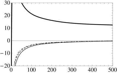
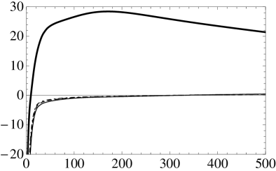
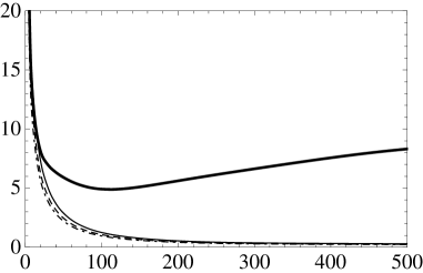
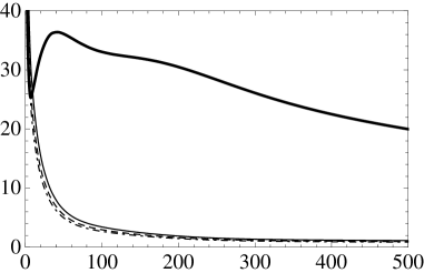
Figure 1: The dependence of hadronic cross sections $\sigma_{1}^{\mathrm{h}}$, $\sigma_{2}^{\mathrm{h}}$ (thick line) and the Coulomb-hadronic interference contributions $\sigma_{1}^{\mathrm{int}}$, $\sigma_{2}^{\mathrm{int}}$ (thin lines) on $T_{\mathrm{lab}}$ for $\bar{p}p$ scattering (upper row) and $\bar{p}n$ scattering (lower row). The interference contribution in the lower row is the interference of the Coulomb $\bar{p}p$ and strong $\bar{p}n$ amplitudes for $\bar{p}d$ scattering. The acceptance angles in the lab frame are $\theta_{\mathrm{acc}}^{(l)}=10\,\mathrm{mrad}$ (solid line), $\theta_{\mathrm{acc}}^{(l)}=20\,\mathrm{mrad}$ (dashed line), $\theta_{\mathrm{acc}}^{(l)}=30\,\mathrm{mrad}$ (dashed-dotted line).

In this section we present our numerical results for the spin-dependent parts of the cross sections of $\bar{p}p$, $\bar{p}n$ and $\bar{p}d$ scattering along with the predictions for the beam polarization degree. Our results for total unpolarized $\bar{p}p$ and $\bar{p}n$ cross sections are in good agreement with all available experimental data. Unpolarized cross sections were studied both theoretically and experimentally by many authors so there is no necessity to present the corresponding Figures here. However, the situation is different for the spin-dependent parts of the cross sections because they were not studied experimentally and different theoretical models provide essentially different predictions. Our predictions for the spin-dependent parts of $\bar{p}p$ cross section were previously presented in Ref. DmitMilSal10 , but we show them here for completeness. The dependence of the spin-dependent parts of the cross section of $\bar{p}p$ and $\bar{p}n$ scattering is shown in Fig. 1. One can see that $\sigma_{2}$ is of the same order for these two processes, but $\sigma_{1}$ for $\bar{p}n$ scattering is smaller than that for $\bar{p}p$ scattering. Note that the sing of the interference contribution to $\bar{p}n$ scattering differs from that to $\bar{p}p$ scattering.

In order to estimate the role of double-scattering mechanism in $\bar{p}d$ scattering we have calculated the total unpolarized $\bar{p}d$ cross section (see Fig. 2-a). One can see that the shadowing effects decrease the total cross section at about $15\%$ in the whole energy region. The line obtained in this work approximates the experimental data Bizzarri74 ; KalogTzan80 ; Burrows70 ; Carroll74 ; HamPunTrippLazNich80 quite accurately.

(a) (b)

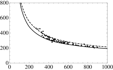
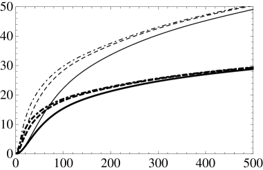
Figure 2: (a) The dependence of the total $\bar{p}d$ cross section on $p_{\mathrm{lab}}$ within the single-scattering approximation (dashed line) and including shadowing effects (solid line). Data are taken from Refs. Bizzarri74 ; KalogTzan80 ; Burrows70 ; Carroll74 ; HamPunTrippLazNich80 . (b) The dependence of the polarization time $t_{0}$ on $T_{\mathrm{lab}}$ for $n=10^{14}\,\mathrm{cm^{-2}}$ and $f=10^{6}\,\mathrm{c^{-1}}$ for $\bar{p}d$ scattering (thick lines) and $\bar{p}p$ scattering (thin lines). The acceptance angles in the lab frame are $\theta_{\mathrm{acc}}^{(l)}=10\,\mathrm{mrad}$ (solid line), $\theta_{\mathrm{acc}}^{(l)}=20\,\mathrm{mrad}$ (dashed line), $\theta_{\mathrm{acc}}^{(l)}=30\,\mathrm{mrad}$ (dashed-dotted line).

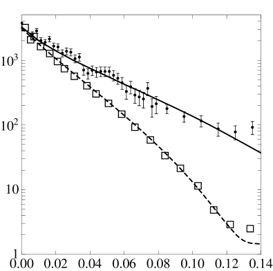
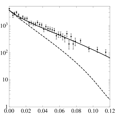
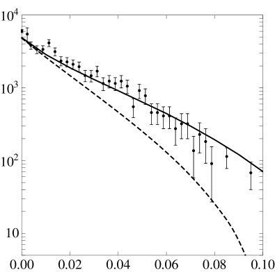
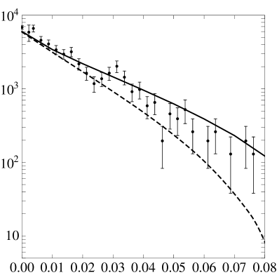
Figure 3: The dependence of elastic (dashed lines) and elastic plus inelastic (solid lines) $\bar{p}d$ differential cross sections on the momentum transfer. Data for the elastic scattering cross section (squares) are taken from Ref. Bruge88 and for elastic plus inelastic cross sections (dots) from Ref. Bizzarri74 .

We also present here the differential elastic ($\bar{p}d\to\bar{p}d$) and elastic plus inelastic ($\bar{p}d\to\bar{p}\,pn$) cross sections (see Fig. 3). These quantities are interesting for us because the double-scattering mechanism is very important for accurate description of non-forward $\bar{p}d$ scattering and we can test the applicability of the Glauber theory to low-energy $\bar{p}d$ scattering comparing our predictions with the existing experimental data. We have included the D-wave contribution with the method described in Ref. FrancoGlauber69 while calculating the elastic differential cross sections. In order to calculate the two form-factors needed by the theory, the numerical values for the deuteron wave function calculated in Ref. Lacombe80 using the Paris model were used. As we expected, the D-wave contribution proved to be significant only for scattering with large momentum transfer because the corresponding form-factor vanishes in the case of forward scattering. Experimental data for the elastic $\bar{p}d$ scattering exist only at $180\,\mathrm{MeV}$ Bruge88 (squares in Fig. 3) and are nicely reproduced by our line. Experimental data for elastic plus inelastic scattering Bizzarri74 are also reproduced quite well, see Fig. 3. The Glauber theory seems to be applicable for the description of unpolarized $\bar{p}d$ cross sections at rather low energies down to $50\,\mathrm{MeV}$.

The spin-dependent parts of the cross section of $\bar{p}d$ scattering were calculated with the double-scattering mechanism taken into account. However, the contribution of D-wave in deuteron wave function was omitted because we expect it to be less important. The spin-dependent parts of $\bar{p}d$ cross section are presented in Fig. 4. The interference contribution to $\bar{p}d$ cross section proved to be less significant in most part of the energy range than it was for $\bar{p}p$ scattering. Shadowing effects turned out to decrease the absolute value of cross sections $\sigma_{1}$ and $\sigma_{2}$ at about $20\div 25\%$ level.

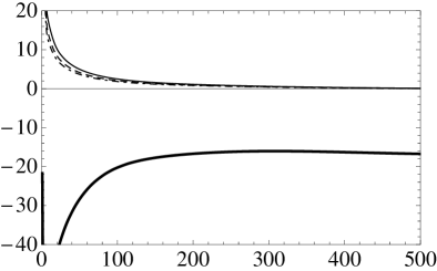
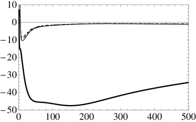
Figure 4: The dependence of $\sigma_{1}$, $\sigma_{2}$ (thick line) and interference contributions $\sigma_{1}^{\mathrm{int}}$, $\sigma_{2}^{\mathrm{int}}$ (thin lines) on $T_{\mathrm{lab}}$ for $\bar{p}d$ scattering. The acceptance angles in the lab frame are $\theta_{\mathrm{acc}}^{(l)}=10\,\mathrm{mrad}$ (solid line), $\theta_{\mathrm{acc}}^{(l)}=20\,\mathrm{mrad}$ (dashed line), $\theta_{\mathrm{acc}}^{(l)}=30\,\mathrm{mrad}$ (dashed-dotted line).

Let us proceed now to the discussion of the polarization buildup. The dependence of the time of polarization $t_{0}$ on the antiproton energy is presented in Fig. 2-b. Note that the number of antiprotons at time $t_{0}$ equals to $14\%$ of the initial number. The dependence of transverse and longitudinal polarization degrees on the antiproton energy is shown in Fig. 5. Analogous results from Ref. DmitMilSal10 for $\bar{p}p$ scattering are also shown in that Figure with the thin lines. One can see that the transverse polarization in the case of deuterium target is smaller than that in the case of hydrogen target. However, it is almost the same for energies below $50\,\mathrm{MeV}$. The picture is different for longitudinal polarization. The longitudinal polarization degree in the case of $\bar{p}d$ scattering is larger for low energies, but it is almost the same as for $\bar{p}p$ scattering in most of energy range concerned.

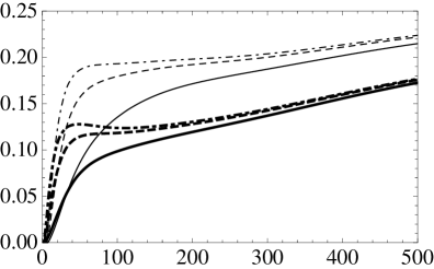
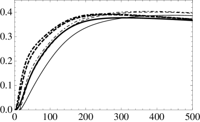
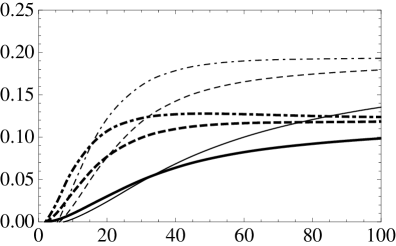
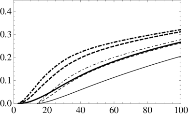
Figure 5: The dependence of $P_{B}(t_{0})$ for $P_{T}=1$ on $T_{\mathrm{lab}}$ for $\boldsymbol{\zeta}_{T}\cdot\boldsymbol{v}=0$ ($P_{\perp}$) and $\left|\boldsymbol{\zeta}_{T}\cdot\boldsymbol{v}\right|=1$ ($P_{\|}$) for $\bar{p}d$ scattering (thick lines) in comparison with $\bar{p}p$ scattering (thin lines). Note that the polarization degree for $\bar{p}p$ scattering is shown with the opposite sign for simplicity. The acceptance angles in the lab frame are $\theta_{\mathrm{acc}}^{(l)}=10\,\mathrm{mrad}$ (solid lines), $\theta_{\mathrm{acc}}^{(l)}=20\,\mathrm{mrad}$ (dashed lines), $\theta_{\mathrm{acc}}^{(l)}=30\,\mathrm{mrad}$ (dashed-dotted lines). Low energy region is shown again in the lower row.

It is important to note that theoretical predictions for the spin-dependent parts of $\bar{p}d$ cross section exhibit fairly strong model dependence. One can compare the predictions for the polarization degree following from the Nijmegen model with that from the Julich models (see Fig. 6). The predictions following from the Julich models are taken from Ref. UzikHaiden11 . Note that they are different from that in Ref. UzikHaiden09 . The polarization degree predicted by the Nijmegen model is about two or three times larger than that predicted by the Julich models and transverse polarization degree even has different sign.

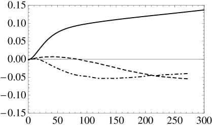
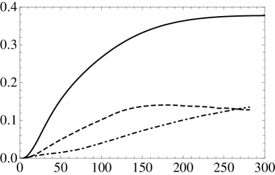
Figure 6: The dependence of $P_{B}(t_{0})$ for $P_{T}=1$ on $T_{\mathrm{lab}}$ for $\boldsymbol{\zeta}_{T}\cdot\boldsymbol{v}=0$ ($P_{\perp}$) and $\left|\boldsymbol{\zeta}_{T}\cdot\boldsymbol{v}\right|=1$ ($P_{\|}$) for $\bar{p}d$ scattering for different models: Nijmegen model (solid line), Julich A model (dashed line) and Julich D model (dashed-dotted line). The acceptance angle in the lab frame is $\theta_{\mathrm{acc}}^{(l)}=10\,\mathrm{mrad}$.

IV Conclusion

We have calculated the cross section of antiproton-deuteron scattering making use of the Nijmegen nucleon-antinucleon potential and the Glauber theory for describing the scattering by a deuteron. Our results show the possibility to describe total and differential unpolarized $\bar{p}d$ cross section in the whole energy region where the experimental data exist. The standard Glauber approach turned out to be sufficient for the precise description of the scattering data. The modifications to account for the spin dependence of the scattering amplitudes and the D-wave part of the deuteron wave function are necessary only for large-angle scattering. The Glauber theory proved to be applicable for $\bar{p}d$ scattering at rather low energies down to $50\,\mathrm{MeV}$.

We have also calculated the spin-dependent parts of $\bar{p}d$ cross section taking shadowing effects into account. Our results indicate that polarized deuterium target can be used instead of the hydrogen target with similar or even higher efficiency. However, one can see fairly strong model dependence of the spin-dependent parts of the cross section. The Nijmegen model predicts higher polarization degree than the other models and this was the case for $\bar{p}p$ scattering too. Only experimental investigation of polarized $\bar{p}p$ or $\bar{p}d$ cross sections can show us what model is closer to the reality.

References

• (1) PAX Collaboration, Technical Proposal for Antiproton-Proton Scattering Experiments with PolarizationarXiv:hep-ex/0505054, 2005.
• (2) A. I. Milstein and V. M. Strakhovenko, Phys. Rev. E 72, 066503 (2005).
• (3) N. N. Nikolaev and F. F. Pavlov, Polarization Buildup of Stored Protons and Antiprotons: Filtex Result and Implications for Pax at Fair, arXiv:hep-ph/0601184, 2006.
• (4) A. I. Milstein, S. G. Salnikov, and V. M. Strakhovenko, Nucl. Instr. and Meth. in Phys. Res. B 266 (2008) 3453.
• (5) P. L. Csonka, NIM 63 (1968) 247.
• (6) V. F. Dmitriev, A. I. Milstein, and V. M. Strakhovenko, Nucl. Instr. and Meth. in Phys. Res. B 266 (2008) 1122.
• (7) V. F. Dmitriev, A. I. Milstein, and S. G. Salnikov, Phys. Lett. B 690 (2010) 427.
• (8) PAX Collaboration, Measurement of the Spin-Dependence of the $\bar{p}p$ Interaction at the AD-RingarXiv:0904.2325, 2009.
• (9) V. Franco and R. J. Glauber, Phys. Rev. 142, 1195 (1966).
• (10) V. Franco and R. J. Glauber, Phys. Rev. Lett. 22, 370 (1969).
• (11) Yu. N. Uzikov and J. Haidenbauer, Phys. Rev. C 79, 024617 (2009).
• (12) M. N. Platonova and V. I. Kukulin, Phys. Rev. C 81, 014004 (2010).
• (13) R. Timmermans, Th. A. Rijken, and J. J. de Swart, Phys. Rev. C 50, 48 (1994).
• (14) M. M. Nagels, T. A. Rijken, and J. J. de Swart, Phys. Rev. D 17, 768 (1978).
• (15) M. Lacombe et al., Phys. Rev. C 21, 861 (1980).
• (16) R. Bizzarri et al., Nuovo Cimento A 22, 225 (1974).
• (17) T. Kalogeropoulos and G. S. Tzanakos, Phys. Rev. D 22, 2585 (1980).
• (18) R. D. Burrows et al., Aust. J. Phys. 23, 819 (1970).
• (19) A. S. Carroll et al., Phys. Rev. Lett. 32, 247 (1974).
• (20) R. P. Hamilton, T. P. Pun, R. D. Tripp, D. M. Lazarus, and H. Nicholson, Phys. Rev. Lett. 44, 1182 (1980).
• (21) G. Bruge et al., Phys. Rev. C 37, 1345 (1988).
• (22) Yu. N. Uzikov and J. Haidenbauer 2011 J. Phys.: Conf. Ser. 295 012087.