The EVN Galactic Plane Survey — EGaPS
Abstract
I present a catalogue of positions and correlated flux densities of 109 compact extragalactic radio sources in the Galactic plane determined from analysis of a 48 hour VLBI experiment at 22 GHz with the European VLBI Network. The median position uncertainty is 9 mas. The correlated flux densities of detected sources are in the range of 20 to 300 mJy. In addition to target sources, nine water masers have been detected, two of them new. I derived position of masers with accuracies 30 to 200 mas and determined velocities of maser components and their correlated flux densities. The catalogue and supporting material is available at http://astrogeo.org/egaps.
keywords:
astrometry – catalogues – instrumentation: interferometers – radio continuum – surveys1 Introduction
The differential very long baseline (VLBI) astrometry became a powerful instrument for a study of the 3D structure and dynamics of our Galaxy. Analysis of differential observations allows us to determine parallaxes of compact radio sources with accuracies down to several tens of microarcseconds, positions with accuracies 0.05 mas and proper motions. The differential astrometry observations are made in the so-called phase referencing mode when radio telescopes of a VLBI network rapidly switch from a target source to a near-by calibrator. Analysis of differential fringe phases allows to dilute the contribution of mismodeled path delays in the atmosphere by the factor of target to calibrator separation in radians, i.e. 20–50 times. Nowadays, observations in the phase-referencing mode are widely used for imaging faint sources. The atmosphere path delay fluctuations limit the integration time, depending on frequency, to 0.2–10 minutes. Phase referencing observations allow to overcome this limit and to integrate the signal for hours. According to Wrobel (2009), 63% of Very Long Baseline Array (VLBA) observations in 2003–2008 were made in the phase referencing mode.
However, the feasibility of phase-referencing observations is determined by the availability of a pool of calibrators with precisely known positions. The first catalogue of source coordinates determined with VLBI contained 35 objects (Cohen & Shaffer, 1971). Since then, hundreds of sources have been observed under geodesy and astrometry VLBI observing programs at 8.6 and 2.3 GHz (X and S bands) using the Mark3 recording system at the International VLBI Service for Geodesy and Astrometry (IVS) network. Analysis of observations in 1980s and 1990s resulted in the ICRF catalogue of 608 sources (Ma et al., 1998). Later, using the VLBA, positions of over 5000 other compact radio sources were determined in the framework of the VLBA Calibrator Survey (VCS) (Beasley et al., 2002; Fomalont et al., 2003; Petrov et al., 2005, 2006; Kovalev et al., 2007; Petrov et al., 2007a), the VIPS program (Helmboldt et al., 2007; Petrov & Taylor, 2011d), the BeSSel Calibrator Survey (Immer et al., 2011), and in the number of on-going programs: the geodetic VLBA program RDV (Petrov et al., 2009), the program of a study of active galaxy nuclea (AGNs) at parsec scales detected with Fermi (Kovalev & Petrov, paper in preparation), the program of observing radio-loud 2MASS galaxies (Petrov, paper in preparation), and the program of observing optically bright quasars (Bourda et al., 2008, 2011; Petrov, 2011c). The use of the Australian Long Baseline Array (LBA) extended the catalogue of calibrators to the zone (Petrov et al., 2011b).
By April 2011, the total number of radio sources with positions determined with the VLBI in the absolute astrometry mode reached 6123 and it continues to grow. On average, the probability of finding a calibrator within a radius of a given position is 97%. However, the density of calibrators in the Galactic plane is still low and an increase of the number of calibrators is badly needed for many VLBI Galactic astronomy projects. Finding extragalactic sources visible through the Galactic plane region is more difficult for several reasons. First, the region is crowded with many galactic objects. Combining independent low-resolution observations at different frequencies makes determination of their spectra problematic due to a risk of source mis-identification. Second, many potential candidates with flat spectra are extended galactic objects, such as planetary nebulae or compact HII regions, that cannot be detected with VLBI. Third, the apparent angular size of extragalactic objects observed through high plasma density near the Galactic plane is broadened by Galactic scattering and cannot be detected at low frequencies on baselines longer than several thousand kilometers.
To address the problem of increasing the density of calibrators within the Galactic plane, we made in 2005–2006 a dedicated blind fringe survey of 2496 objects with the VERA (Petrov et al., 2007b) radio interferometer at the K-band (22 GHz). Those sources which were detected with the VERA were re-observed with the VLBA in 2006 at K-band in the framework of the VGaPS campaign (Petrov et al., 2011a). These observations allowed to determine positions of 176 new sources within 6°of the Galactic plane with the median accuracy of 0.9 mas. The detection limit of VERA was 200–300 mJy, the detection limit of the follow-up VLBA observations was 70–90 mJy depending on a baseline111The K-band receivers at the VLBA stations were upgraded in 2007, after these observations, which improved the sensitivity of the array at 24 GHz at the same recording rate by a factor of 2 according to Walker et al. (2008).. Independently, a team led by Mark Reid searched for Galactic plane calibrators in 2010 using the VLBA in the framework of BeSSeL project and reported detection of 198 sources Immer et al. (2011), 82 of them are new.
In this paper I present results from a 48 hour experiment at the European VLBI Network (EVN) observed in October 2009 called the EVN Galactic Plane Survey (EGaPS). The goal of this experiment is to further increase the calibrator source density in the zone within 6°of the Galactic plane and with declinations . Using highly sensitive antennas, I was able to detect sources as weak as 20 mJy, a factor of 4 weaker than in the prior VGaPS campaign. These calibrators are aimed to be used for Galactic astronomy projects. The selection of candidate sources and the scheduling strategy is discussed in section 2. The station setups during the observing sessions is described in section 3. The correlation and post-correlation analysis is discussed in section 4. The catalogue of source positions and correlated flux densities is presented in section 6. An error analysis of observations, including evaluation of systematic errors, is given in subsection 4.3, and the results are summarized in section 7.
2 Candidate source selection
In the past, the list of bright compact sources detected at the Very Large Array (VLA) and/or MERLIN served as a pool for candidates for VLBI calibrator surveys. Almost all these objects have been already surveyed with the VLBA. Since the combined catalogue of sources observed in the absolute astrometry mode is complete at the 150–200 mJy level, new calibrators should be relatively faint objects. Most all-sky surveys at frequencies higher than 2 GHz are either incomplete and/or not deep enough. As a result, information about spectral indices is sparse and is often unreliable. For this reason, it is more difficult to find remaining good flat spectrum candidate sources.
New calibrator candidates were found by analyzing 395 radio astronomical catalogues using the CATS database (Verkhodanov et al., 1997). The database includes NVSS (Condon et al., 1998), CLASS (Myers et al., 2003), CRATES (Healey et al., 2007), ATCA survey at 20 GHz (Murphy et al., 2010), and many other catalogues. Initially, I selected 1100 sources which satisfy the following criteria:
-
•
were not observed previously with VLBI;
-
•
have galactic latitude ;
-
•
have declination ;
-
•
have at least two measurements of their flux density that allow estimation of their spectral indices at frequencies higher than 2 GHz;
-
•
have single-dish flux densities extrapolated to 22 GHz 80mJy;
-
•
have spectral indices flatter than ().
The majority of these sources were selected by cross-identification of the NVSS and GB6 (Gregory et al., 1996) catalogues. Then I scrutinized the source spectra and rejected approximately 50% of the sources with unreliable spectra or the objects known as galactic sources. The remaining list contains 559 candidates.
2.1 Observation scheduling
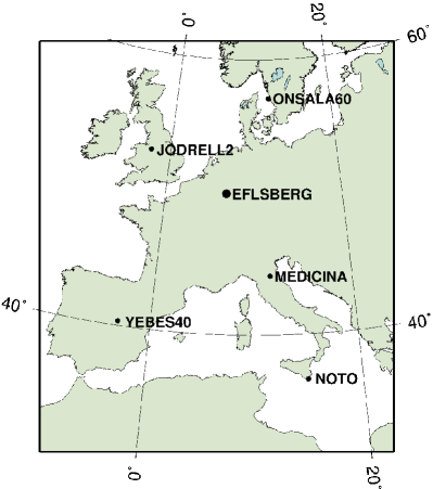
The following stations were scheduled for 48 hour observations: eflsberg, jodrell2, medicina, noto, onsala60, and yebes40m (see Figure 1. The observation schedule was prepared with the software program sur_sked. The scheduling goal was to observe each target source at all antennas of the array in 2 scans of 120 seconds each.
The scheduling algorithm found the sequence of sources that minimized slewing time. The minimum time between consecutive observations of the same source was set to 4 hours. For deciding which source to put into the schedule, the algorithm calculated the elevation of each candidate object, the slewing time, the time interval between previous observation of the same source, and the ratio of the remaining visibility time to the total visibility time. For each source with the elevation exceeding 15°above the horizon, a score was computed. The score is the function of slewing time, the ratio of the remaining visibility time to the total visibility time, and the time interval from the previous observation. A source with the highest score was put into the schedule and then the procedure was repeated.
Every 1.5 hr a burst of 4 strong compact sources with known maps from the K/Q survey (Lanyi et al., 2010) was observed: two strong objects at elevation angles 10– and two strong objects at elevations 50–. The purpose of scheduling these calibrators was a) to allow estimation of the troposphere path delay in zenith direction; b) to evaluate the atmosphere opacity; c) to use them for complex bandpass calibration; d) to provide a strong connection between the new catalogue to the old catalogue of compact sources.
The schedule had 369 target objects and 69 calibrators. Among target sources, 344 objects were observed in 2 scans and 25 sources were observed in 1 scan.
3 Observations
Observations took place on 2009 October 27–29. Eight intermediate frequencies (IF), both upper and lower sub-band in the range of [22.09999, 22.35599] GHz were observed in a single left circular polarization with two bits per sample. The data were recorded with the Mark-5 system with the aggregate rate 1024 Mbit/sec. The contiguous frequency setup is far from optimal for an absolute astrometry experiment that utilizes group delays, since the uncertainties of a group delay at a given signal-to-noise ratio (SNR) is reciprocal to the root mean squares (rms) of IFs. Two stations, medicina and onsala60 could record within 720 MHz, three stations equipped with the VLBA data acquisition system, eflsberg and noto yebes40m, could record within 500 MHz and jodrell2 could record within 160 MHz. Spreading IFs over 500 MHz would reduce group delay uncertainty by a factor of 2.4 at all baselines, except jodrell2 where it would increase the uncertainty by a factor of 2 since some channels will be missing. However, in order to record a band wider than 256 MHz, the local oscillator (LO) frequency should be changed with respect to those that are used in other EVN experiments. This would require manual intervention. When I realized that for logistical reasons there is a high risk that this change would not be made at some stations, which could ruin the experiment, I fell back to the contiguous frequency setup.
Station yebes40m lost first 7 hours of the experiment because of the Mark-5B failure. The system temperature of yebes40m was around 210 K during next three hours because the vertex was closed. It dropped to the normal range of 60-100 K when the operator noticed it and opened the vertex. Station jodrell2 did not show fringes in IF11–IF16.
4 Data analysis
Analysis of the EGaPS data is similar to that performed for the VLBA Galactic plane calibrator survey. Detailed description of the analysis technique can be found in Petrov et al. (2011a). Here the analysis procedure is briefly outlined.
4.1 Data correlation and post-correlation analysis
The data were correlated at the Bonn DiFX software correlator Deller et al. (2007) with the accumulation periods of 0.12 s and with the spectral resolution of 125 KHz. These correlation parameters provided the field of view over , comparable with the width of the beam of eflsberg radio telescope. I anticipated the a priori source coordinates of some sources may be wrong at the arc-minute level due to source mis-identification.
The correlator generates the spectrum of the cross-correlation function that was written in the format compliant with the FITS-IDI specifications (Greisen, 2009). Data analysis was performed with software 222Available at http://astrogeo.org/pima.. At the first step, the fringe amplitudes were corrected for the signal distortion in the sampler. Observations of strong sources were used for deriving complex bandpasses. Since in 2010 the DiFX correlator did not have an ability to extract phase calibration signal from the data, no phase calibration was applied. After that, the group delay, phase delay rate, group delay rate, and fringe phase were determined for each scan at each baseline using the fringe fitting procedure. These estimates maximize the sum of the cross-correlation spectrum coherently averaged over all accumulation periods of a scan and over all frequency channels in all IFs. After the first run of fringe fitting, 8 observations at each baseline with the strongest SNR were used to adjust the station-based complex bandpass corrections, and the procedure of computing group delays was repeated with the bandpass applied.
Then the results of fringe fitting were exported to the VTD/post-Solve VLBI analysis software333Available at http://astrogeo.org/vtd. for interactive processing group delays with the SNR high enough to ensure the probability of false detection less than 0.001. Analysis of the probability distribution function of achieved SNR allowed me to find that the probability of a false detection in our experiment is less than 0.001 when SNR. Theoretical path delays were computed according to the state-of-the art parametric model as well as their partial derivatives. The model included the contribution of the ionosphere to group delay and phase delay rate computed using the total electron contents maps derived from analysis of Global Positioning System (GPS) observations by the analysis center CODE (Schaer, 1998). Small differences between group delays and theoretical path delay as well as between the measured and theoretical delay rate were used for an interactive estimation of corrections to a parametric model that describes the observations with least squares (LSQ). Coordinates of target sources, positions of all stations, except the reference one, parameters of the splines that describe corrections to the a priori path delay in the neutral atmosphere in the zenith direction for all stations, and parameters of another splines that describe the clock function were solved for in a single LSQ solution using group delays. Outliers were identified and temporarily suppressed, and additive corrections to weights of observables were determined. Then the fringe fitting procedure was repeated for outliers with phase delay rates and group delays evaluated in a narrow window around the expected value computed on the basis of results of the previous LSQ solution. New estimates of group delays for points with probabilities of false detection less than 0.1, which corresponds to the SNR for the narrow fringe search window, were used in the next step of the interactive analysis procedure. For observations detected with the narrow window search the status outlier was lifted and they were selected back for using in further analysis. Parameter estimation, elimination of remaining outliers and adjustments of additive weight corrections was then repeated. In total, group delays of 2471 observations out of 11675 scheduled were used in the solution. There were 178 sources detected in 3 to 28 observations, including 109 target sources and 69 calibrators.
4.2 Source position determination
Results of the interactive solution provided a clean dataset of group delays with updated weights from the EGaPS experiment. The dataset that was used for the final parameter estimation utilized all dual-band S/X data acquired under absolute astrometry and space geodesy programs from April 1980 through February 2011 and included the K-band data from the EGaPS experiment, in total 8 million observations. The estimated parameters are right ascensions and declination of all sources, coordinates and velocities of all stations, coefficients of B-spline expansion of non-linear motion for 16 stations, coefficients of harmonic site position variations of 48 stations at four frequencies: annual, semi-annual, diurnal, semi-diurnal, and axis offsets for 67 stations. They were adjusted using all the data. Estimated parameters also included Earth orientation parameters for each observing session, parameters of clock function and residual atmosphere path delays in the zenith direction modeled with the linear B-spline with interval 60 and 20 minutes respectively. All parameters were estimated in a single LSQ run.
The system of LSQ equations has an incomplete rank and defines a family of solutions. In order to pick a specific element from this family of solutions, I applied the no-net rotation constraints on the positions of 212 sources marked as “defining” in the ICRF catalogue (Ma et al., 1998) that required the positions of these source in the new catalogue to have no rotation with respect to the position in the ICRF catalogue. No-net rotation and no-net-translation constraints on site positions and linear velocities were also applied. The specific choice of identifying constraints was made to preserve the continuity of the new catalogue with other VLBI solutions made during last 15 years.
The global solution sets the orientation of the array with respect to the ensemble of extragalactic remote radio sources. The orientation is defined by the continuous series of Earth orientation parameters and parameters of the empirical model of site position variations over 30 years evaluated together with source coordinates. Common sources observed in the EGaPS experiment as amplitude calibrators provided a connection between the new catalogue and the old catalogue of compact sources.
A valuable by-product of analysis of EGaPS observations is estimates of jodrell2 positions (see Table 1). This is the second experiment with participation of this station under astrometry or geodesy programs. The previous EVN experiment TP001 carried out on 2000 November 23 was made at 5 GHz with the bandwidth spread over 108 MHz (Charlot et al., 2002). Comparison of results of reanalysis of TP001 and EGaPS made using exactly the same a priori model and parameter estimation technique showed that the differences between jodrell2 position reduced to the J2000.0 epoch using the velocities predicted by the NNR-NUVEL1A plate tectonic model (DeMets et al., 1994) are 38, 20, and 9 mm at X, Y and Z coordinate respectively. Although position of jodrell2 from the 5 GHz observations with formal uncertainties 10–20 mm suffered from residual errors in modeling path delay through the ionosphere which are 20 times greater than at 22 GHz, the differences in positions are within 1–2 reported uncertainties.
| X | 3822846.633 | 0.026 | |
|---|---|---|---|
| Y | -153802.071 | 0.009 | |
| Z | 5086286.064 | 0.036 |
4.3 Position error analysis
The formal uncertainties of semi-major axis of the error ellipses of position estimates of 109 target sources range from 2 to 60 mas with the median value of 8 mas. They are based on the error propagation law of group delay uncertainties derived by the fringe fitting procedure.
Including in observing schedule a considerable number of calibrator sources with positions known at the sub-mas level facilitated the error analysis. In order to evaluate the level of systematic errors, I used a similar technique that was developed for processing VGaPS observations. The list 69 calibrators was ordered in increasing their right ascensions and split it into two subsets with even and odd indices. I made two special global solutions using all the data from 1980 through 2011. I excluded in solution A calibrators with even indices from all experiments, but the EGaPS. I excluded in solution B calibrators with odd indices from all experiments, but the EGaPS. I compared positions of calibrator sources from solutions A and B with their position from the dual-band global solution C that used all sources in all experiments, except the EGaPS. Positions of sources from solution C is determined with accuracies 0.1–0.3 mas and can be considered as true for the purpose of this comparison.
The wrms of the differences of 69 calibrator sources from special solutions A and B and the reference solution C are 1.8 mas in declinations and 3.7 mas in right ascensions scaled by with per degree of freedom 1.3 and 3.3 respectively. If to add in quadrature to uncertainties in right ascensions and declinations the noise with the standard deviations 4.0 mas and 1.0 mas respectively, the per degree becomes close to 1. Therefore, I inflated the reported uncertainties in right ascensions and declinations of target sources by 4.0 mas and 1.0 mas in quadrature.
4.4 Data analysis: correlated flux density determination
Each detected source has from 3 to 30 observations, with the median number of 8. The dataset is too sparse to produce meaningful images. In this study I limited my analysis with mean correlated flux density estimates in two ranges of lengths of the baseline projections onto the plane tangential to the source without inversion of calibrated visibility data. Information about the correlated flux density is needed for evaluation of the required integration time when an object is used as a phase calibrator.
Analysis of system temperature measurements revealed variations with time and with elevation angle. The measured system temperature is considered as a sum of two terms: the receiver temperature and the contribution of the atmosphere:
| (1) |
where is the average temperature of the atmosphere, is the atmosphere opacity, and is the wet mapping function: the ratio of the neutral atmosphere non-hydrostatic path delay at the elevation to the atmosphere non-hydrostatic path delay in the zenith direction. I omitted in expression 1 the ground spillover term that was not determined for these antennas. Both, the receiver temperature and the atmosphere opacity, depend of time. Since in astrometric analysis I estimated for each station the non-hydrostatic component of the atmosphere path delay in the zenith direction which is closely related to the integrated column of the water vapor, I can use these estimates for modeling time dependence of the opacity. I present the system temperature as
| (2) |
where and are empirical coefficients that relate the opacity and the estimates of the atmosphere path delay, is the estimate of the non-hydrostatic atmosphere path delay, is the B-spline of the first degree with the pivotal element , and are the coefficients of the expansion the receiver temperature into B-spline basis. I set to 280K, and evaluated the coefficients of the receiver temperature and regression parameters and by fitting them into measurements of system temperatures with the use of the non-linear LSQ. Parameter describes the possible bias between estimates of the integrated water vapor contents and the non-hydrostatic path delay in the zenith direction. The system temperature divided by is free from absorption in the atmosphere and equivalent to that at the top of the atmosphere.
The root mean squares (rms) of residuals of the empirical model of the system temperature are in the range of 2–8 K. The time variations of were within 10 K at eflsbereg, jodrells2, medicina, and noto. The was around 180 K during first 3 hours at yebes40m and then suddenly dropped to 30 K and after that stayed stable. The at onsala60 was unstable during the entire experiment and varied in the range 40–250 K.
The fringe amplitudes were calibrated by multiplying them by the system temperature reduced to the top of the atmosphere and dividing by the elevation dependent a priori gain.
The a priori antenna gain and/or the term may have a multiplicative error. The corrections to antenna gain were evaluated by fitting the correlated amplitude to the flux density of sources with known brightness distributions. Among sources used as amplitude calibrators, brightness distributions are publicly available444The database of brightness distributions, correlated flux densities, and images of compact radio sources produced with VLBI is accessible from http://astrogeo.org/vlbi_images for 45 objects from the K/Q survey and the VGaPS observing campaigns.
For each used amplitude calibrator observation with known brightness distribution in the form of CLEAN components I predicted the correlated flux density as
| (3) |
where is the correlated flux density of the th CLEAN component with coordinates and with respect to the center of the image, and and are the projections of the baseline vectors on the tangential plane of the source.
Then I built a system of least square equations for all observations of calibrators with known brightness distributions used in the astrometric solution:
| (4) |
and after taking logarithms from left and right hand sides solved for corrections to gains for all stations using LSQ. Finally, I applied corrections to gain for observations of all other sources.
The gain correction was in the range 0.7–1.3 for all antennas, except jodrell2. The correction to jodrell2 gain was 6.9, and its system equivalent flux density (SEFD) at elevations higher than 50°was around 7000 K.
The detection limit varied significantly between the baselines. Sources as weak as 13–16 mJy had the and therefore, were detected at the most sensitive baseline eflsberg/yebes40m. The detection limit at baselines eflsberg/medicina and eflsberg/noto was in the range of 25–30 mJy, at the baseline eflsberg/onsala60 was 30–40 mJy, and at the baselines eflsberg/jodrell2 and medicina/noto was 60–70 mJy.
5 Data analysis: H2O maser sources
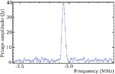
During scrutinizing the cross-correlation spectra, I found several objects with very strong peaks in the IF9, for example object 0221618 at baseline medicina/onsala60 (see Figure 3).
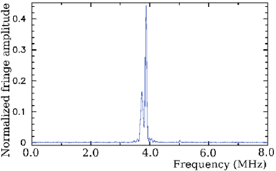
This feature of the fringe spectrum is interpreted as an emission from a water maser. The peak frequency of the cross-spectrum is shifted within several megahertz due to a relative motion of the maser with respect to the geocenter. Although this project was not targeted on maser investigation, nevertheless, I decided to systematically search for masers in the data, determine their coordinates and parameters of their spectra.
Processing the data from narrow-band sources differs significantly from processing the data from continuum sources. I searched for masers by running 31 trial fringe fitting with spectral window of 1 MHz within the IF9 in the range of 22.22799–22.24399 GHz. Other spectral constituents were masked out. The spectral window was shifted at 0.5 MHz after each run. Since the maser has emission only within a narrow band, suppressing the spectrum beyond the search window improved the SNR considerably, because the amount of noise is reduced, but the power of the signal remained the same. I searched for objects with the peak fringe amplitude higher than 4 times the spectrum rms. This approach helped to discover 9 maser objects. After the signal from masers was detected at at least one baseline, the spectrum filter was narrowed down even further to reduce the contribution of noise away from the spectral lines. This allowed me to increase the number of detections at other baselines.
The frequency resolution of the cross-spectrum, 125 KHz, that correspond to the Doppler velocity resolution 1.7 km s-1, is not sufficient to resolve the water maser spectral line. The scans with 7 out of 9 detected masers were re-correlated with 16 times higher spectral resolution of 7.8 KHz, which corresponds to the Doppler velocity resolution 0.1 km s-1. Two other masers, 2130556 and 2247596 were discovered after the recorded data were recycled, and it was too late to re-correlate them.
I smoothed the cross-spectrum and fitted the preliminary model of the amplitude spectrum of maser emission using an iterative non-linear LSQ procedure. Here is the peak amplitude of the component, its frequency, is the parameter of the line width, and is the rest H frequency. After determining a satisfactory preliminary model of the smoothed spectrum, I fitted the final model using the raw cross-spectrum. Since masers are not point-like objects, but usually a conglomerate of tens or even hundreds spots, the correlated flux density at different parts of the -plane differs considerably due to beatings from different components. Using only 10–20 points at the -plane is not sufficient for an image reconstruction. Therefore, I restricted the amplitude analysis to determination of the minimal and maximum correlated flux densities of detected components at different baselines.
The fringe fitting process cannot provide a meaningful estimate of a group delay for a narrow-band source. Therefore, I resorted to using phase delay rates for determining the source positions. A phase delay rate over 2 minutes of integration time at 1024 Gb/s recording rate has the uncertainty due to the thermal noise of order . However, unmodeled short-term atmosphere path delay fluctuations limit the accuracy of modeling the phase delay rate usually at a level of 5–10. The uncertainty of the phase delay rate equivalent to group delay, (where at is the nominal Earth rotation rate) SNR=10 is 300 ps if to take into account only thermal noise, and 1400 ps if to consider the contribution of the atmosphere path delay rate. The uncertainty of group delay at SNR=10 in our experiment is around 200 ps, i.e. a factor 7 better. If to use only phase delay rates, the adjustments to nuisance parameters, such as atmosphere path delays in zenith direction, station positions, and clock functions, will be determined less precisely than from the group delay solution and they will affect estimate of source coordinates. In order to alleviate the effect of poorly determined nuisance parameters on estimates of maser positions, I ran a special solution with observation equations using both group delay and phase delay rates for all detected sources, continuum spectrum objects and masers. The phase delay rate had zero weight for continuum sources and group delay had zero weight for maser sources.
Positions of maser sources and their uncertainties are presented in Table 2. This table also contains the peak minimum and maximum correlated flux densities for each component of a maser source over observations at different baselines and the velocity with respect to the local system of rest (LSR) assuming the barycenter of the Solar system moving with the speed of 20 km-1s towards the direction with right ascension and declination . The table contains the full-width half-maximum (FWHM) of the line profile and the minimum and maximum correlated flux densities integrated over the line profile: . For two sources that were correlated only with the low spectral resolution, the low limit of their peak correlated flux densities and the low limit of the FWHM of their line profiles are presented.
| (1) | (2) | (3) | (4) | (5) | (6) | (7) | (8) | (9) | (10) | (11) | (12) | (13) | (14) |
|---|---|---|---|---|---|---|---|---|---|---|---|---|---|
| 0221618 | W3(2) | 02219+6152 | 02 25 40.672 | 0.13 | +62 05 54.06 | 0.08 | 1 | 24.6 | 52.1 | 0.4 | 5.7 | 12.1 | |
| 2 | 6.0 | 28.3 | 0.3 | 1.1 | 5.9 | ||||||||
| 3 | 13.7 | 1039.1 | 0.4 | 3.3 | 275.5 | ||||||||
| 4 | 4.4 | 393.4 | 0.6 | 0.8 | 120.3 | ||||||||
| 5 | 5.6 | 324.0 | 0.5 | 0.9 | 87.7 | ||||||||
| 6 | 15.8 | 346.7 | 0.5 | 4.5 | 102.5 | ||||||||
| 7 | 12.1 | 85.7 | 0.4 | 2.5 | 26.1 | ||||||||
| 8 | 7.4 | 42.6 | 0.4 | 1.5 | 11.4 | ||||||||
| 1907082 | 19074+0814 | 19 09 49.847 | 0.03 | +08 19 45.28 | 0.20 | 1 | 7.5 | 19.4 | 0.5 | 2.1 | 5.0 | ||
| 2 | 1.8 | 1.8 | 0.4 | 0.4 | 0.4 | ||||||||
| 1920143 | W51 W | 19209+1421 | 19 23 11.224 | 0.03 | +14 26 45.80 | 0.11 | 1 | 6.9 | 9.0 | 0.6 | 1.8 | 3.8 | |
| 2 | 2.8 | 26.5 | 0.5 | 0.7 | 7.4 | ||||||||
| 3 | 3.1 | 9.9 | 0.5 | 0.7 | 3.8 | ||||||||
| 4 | 8.8 | 34.2 | 0.5 | 2.7 | 10.2 | ||||||||
| 5 | 1.9 | 5.1 | 0.4 | 0.4 | 1.4 | ||||||||
| 1923151 | 19230+1506 | 19 25 17.907 | 0.06 | +15 12 24.46 | 0.17 | 1 | 1.6 | 1.8 | 0.5 | 0.4 | 0.5 | ||
| 2 | 5.3 | 5.3 | 0.8 | 2.4 | 2.4 | ||||||||
| 3 | 1.7 | 4.1 | 0.4 | 0.5 | 0.8 | ||||||||
| 4 | 2.6 | 3.6 | 0.4 | 0.6 | 0.8 | ||||||||
| 2011360 | 20116+3605 | 20 13 34.296 | 0.06 | +36 14 54.36 | 0.06 | 1 | 8.9 | 45.4 | 0.3 | 1.6 | 7.9 | ||
| 2107521 | WB43 | X2107+521 | 21 09 21.717 | 0.04 | +52 22 37.05 | 0.03 | 1 | 1.5 | 55.6 | 0.4 | 0.3 | 16.0 | |
| 2 | 2.2 | 41.0 | 0.4 | 0.5 | 16.6 | ||||||||
| 3 | 2.5 | 63.4 | 0.6 | 0.7 | 26.1 | ||||||||
| 4 | 6.5 | 17.3 | 0.4 | 1.3 | 3.8 | ||||||||
| 5 | 5.3 | 25.1 | 0.4 | 1.1 | 6.5 | ||||||||
| 6 | 2.3 | 40.1 | 0.4 | 0.6 | 7.5 | ||||||||
| 7 | 1.6 | 37.0 | 0.3 | 0.3 | 7.7 | ||||||||
| 8 | 1.3 | 38.1 | 0.3 | 0.3 | 7.5 | ||||||||
| 9 | 2.3 | 99.9 | 0.3 | 0.4 | 20.3 | ||||||||
| 10 | 2.8 | 16.1 | 0.3 | 0.6 | 2.8 | ||||||||
| 2130556 | 21306+5540 | 21 32 12.444 | 0.07 | +55 53 49.64 | 0.04 | 1 | 0.8 | 0.6 | 25.3 | ||||
| 2247596 | S146 | X2247+596 | 22 49 31.474 | 0.06 | +59 55 41.91 | 0.03 | 1 | 1.1 | 0.8 | 11.6 | |||
| 2254617 | Cep A | 22543+6145 | 22 56 17.988 | 0.06 | +62 01 49.40 | 0.04 | 1 | 2.7 | 34.8 | 0.4 | 0.5 | 7.7 | |
| 2 | 3.2 | 31.4 | 0.5 | 0.6 | 10.7 | ||||||||
| 3 | 2.9 | 37.4 | 0.6 | 0.5 | 15.6 | ||||||||
| 4 | 11.7 | 20.6 | 0.4 | 2.3 | 4.3 | ||||||||
| 5 | 4.5 | 5.2 | 0.3 | 0.9 | 0.9 | ||||||||
| 6 | 21.7 | 40.1 | 0.4 | 5.0 | 11.8 | ||||||||
| 7 | 5.7 | 111.8 | 0.5 | 1.3 | 47.9 | ||||||||
| 8 | 3.1 | 217.7 | 0.3 | 0.6 | 36.8 | ||||||||
| 9 | 5.0 | 8.4 | 0.5 | 1.3 | 1.9 | ||||||||
| 10 | 4.9 | 5.4 | 0.3 | 1.0 | 1.1 | ||||||||
| 11 | 4.3 | 7.5 | 0.5 | 0.8 | 2.8 |
5.1 Comments on individual masers
Cep A. Curiel et al. (2002) reported detection of a 2 mJy continuum source at 7 mm in the Cep A complex from VLA observations in 1996. Position of that source, which they labeled as VLA-mm, is with the uncertainty . Our position of Cep A water maser coincides within with the position of VLA-mm source. Moscadelli et al. (2009) determined position of the methanol maser associated with this object using phase-referencing VLBI: and with sub-milliarcsecond accuracy. Their position of the methanol maser is within from the water maser.
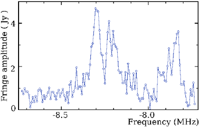
1923151 is a new discovery. Its spectrum is shown in Figure 4. It is associated with IRAS192301506 ( away) and WISE J192517.93151225.0 ( away), within 1–2 of position uncertainty of these catalogues.
6 The EGaPS catalogue
| Class | IVS | IAU | Right ascension | Declination | Corr | # Obs | Total | Unres | |||
|---|---|---|---|---|---|---|---|---|---|---|---|
| (1) | (2) | (3) | (4) | (5) | (6) | (7) | (8) | (9) | (10) | (11) | |
| U | 0002576 | J00045754 | 00 04 50.263646 | 57 54 57.75926 | 16.9 | 18.9 | -0.159 | 4 | |||
| N | 0008657 | J00116603 | 00 11 38.823302 | 66 03 38.51426 | 27.0 | 4.9 | 0.245 | 7 | |||
| C | 0017627 | J00196300 | 00 19 47.644959 | 63 00 46.63373 | 28.8 | 4.9 | 0.094 | 8 | |||
| N | 0133602 | J01366032 | 01 36 56.806879 | 60 32 05.06934 | 24.7 | 6.2 | -0.159 | 7 | |||
| U | 0158623 | J02016237 | 02 01 52.980387 | 62 37 57.12279 | 48.4 | 11.0 | -0.305 | 4 | |||
| N | 0245620 | J02486214 | 02 48 58.890890 | 62 14 09.66282 | 19.8 | 5.8 | -0.296 | 6 | |||
| N | 0252574 | J02565736 | 02 56 29.004510 | 57 36 42.45601 | 12.9 | 4.5 | -0.013 | 9 | |||
| U | 0313531 | J03175318 | 03 17 01.346538 | 53 18 27.51902 | 19.8 | 9.8 | 0.225 | 4 | |||
| C | 0334565 | J03385640 | 03 38 36.909254 | 56 40 50.05381 | 11.9 | 3.1 | 0.034 | 11 | |||
| N | 0339573 | J03435729 | 03 43 44.815127 | 57 29 08.52764 | 26.0 | 8.6 | 0.174 | 5 | |||
| N | 0357457 | J04004554 | 04 00 34.574245 | 45 54 24.05505 | 11.1 | 5.4 | 0.204 | 7 |
Table 3 displays 12 out of 109 rows of the EGaPS catalogue of source positions. The full table is available in the electronic attachment. Column 1 contains the class of the source, columns 2 and 3 contain the J2000 and B1950 IAU names; column 4, and 5 contain right ascensions and declinations of sources. Columns 6 and 7 contain position errors in right ascension (without multiplier ) with noise 4.0 mas/ and 1.0 mas added in quadrature to formal position uncertainties in right ascension and in declination respectively. Column 8 contains correlation coefficients between right ascension and declination, column 9 contains the total number of observations used in position data analysis. Columns 10 and 11 contain the median estimates of the correlated flux density over all experiment of the source in two ranges of baseline projection lengths: 0–67 (projections shorter than 900 km) and 100-170 — projections longer than 1350 km. If there were no scheduled observations at the range of the baseline projection lengths, then is put in the table cell.
7 Summary
I determine positions of 109 compact extragalactic sources that are within 6°of the Galactic plane with declinations . Observations were made at a six-element array of the Europearn VLBI Network. As a result of these observations, the total number of calibrator sources with precisely known positions in this region grew from 322 to 431. The semi-major axis of position errors range from 5 to 60 mas, and the median position uncertainty is 9 mas.
Among detected sources, nine water masers in our Galaxy were identified, two of them new. The date for seven these objects were re-correlated with the spectral resolution of 0.1 km/s. I determined position of masers from delay rates with accuracies 30–200 mas, determined velocities of components and their correlated flux densities.
I also obtained estimates of source correlated flux densities. The correlated flux densities of extragalactic sources range from 20 to 300 mJy with the median value of 55 mJy.
The results of this campaign are somewhat disappointing. First, the median position accuracy is one order of magnitude worse than in a similar campaign with the VLBA. Several factors contributed to the increase of uncertainties in source positions. First, the unfavorable frequency setup resulted in an increase of group delay uncertainties by a factor of 2.4. Retrospectively, I should admit that more efforts should be put in order to resolve logistical issues with LO frequency changes. Second, the size of the EVN network used in this experiment is a factor of 3 less than the size of the VLBA network. Third, the sources in EGaPS campaign are a factor of 3 weaker than in the VGaPS campaign.
The detection rate, 30% is significantly lower than in other survey experiments. For comparison, the detection rate in the VGaPS experiment among sources in the Galactic plane preselected with VERA observations was 76% and 36% among the sources selected on the basis of their spectral index. Apparently, the efficiency of sources selection based on the spectral index is at a level of 30-40% in the Galactic plane. About 1/3 detected sources have the correlated flux density below 40 mJy which makes their use as phase calibrator problematic. This indicates that the source selection strategy should be revised if a similar survey will be made in the future.
8 Acknowledgments
I made use of the database CATS of the Special Astrophysical Observatory. I used in our work the dataset MAI6NPANA provided by the NASA/Global Modeling and Assimilation Office (GMAO) in the framework of the MERRA atmospheric reanalysis project. It is my pleasure to thank Yury Kovalev, David Graham, Richard Porcas, and Cormac Reynolds for useful suggestions that contributed to the success of the experiment. I would like to thank Alessandra Bertarini and Helge Rottmann for prompt re-correlation scans with masers. The European VLBI Network is a joint facility of European, Chinese, South African, Russian, and other radio astronomy institutes funded by their national research councils. This publication makes use of data products from the Wide-field Infrared Survey Explorer, which is a joint project of the University of California, Los Angeles, and the Jet Propulsion Laboratory/California Institute of Technology, funded by the NASA.
References
- Beasley et al. (2002) Beasley A. J., Gordon D., Peck A. B., Petrov L., MacMillan D. S., Fomalont E. B., Ma C., 2002, ApJS, 141, 13
- Bourda et al. (2008) Bourda, G., Charlot, P., & Le Campion, J.-F. 2008, A&A, 490, 403
- Bourda et al. (2011) Bourda, G., Collioud, A., Charlot, P., Porcas, R. W., & Garrington, S. T. 2011, A&A, 526, A102
- Charlot et al. (2002) Charlot P. et al., 2002, in Proc. of the 6th European VLBI Network Symposium, 9 http://www.mpifr-bonn.mpg.de/div/vlbi/evn2002/book/PCharlot.pdf
- Cohen & Shaffer (1971) Cohen M. H. & Shaffer D. B., 1971, AJ, 76, 91.
- Condon et al. (1998) Condon, J. J., Cotton, W. D., Greisen, E. W., Yin, Q. F., Perley, R. A., Taylor, G. B., Broderick, J. J. 1998, AJ, 115, 1693
- Curiel et al. (2002) Curiel, S., et al., 2002, ApJ, 564L
- Deller et al. (2007) Deller, A. T., Tingay, S. J., Bailes, M., West, C. 2007, PASP, 119(853), 318
- DeMets et al. (1994) DeMets, C., Gordon, R., Argus, D., Stein, S., 1994, Geophys. Res. Lett. 21, 2191 2194
- Fomalont et al. (2003) Fomalont E., Petrov L., McMillan D. S., Gordon D., Ma C. 2003, AJ, 126, 2562
- Gregory et al. (1996) Gregory, P. C., Scott, W. K., Douglas, K., & Condon, J. J. 1996, ApJS, 103, 427
- Greisen (2009) Greisen E. W., 2009, AIPS Memo, 114 ftp://ftp.aoc.nrao.edu/pub/software/aips/TEXT/PUBL/ AIPSMEM114.PDF
- Healey et al. (2007) Healey, S. E.. Romani, R. W., Taylor, G.B., Sadler, E. M.; Ricci, R., Murphy, T.; Ulvestad, J. S.; Winn, J. N. 2007, ApJS, 171, 61
- Helmboldt et al. (2007) Helmboldt, J. F., et al., 2007, ApJ, 2007ApJ, 658, 203
- Immer et al. (2011) Immer, K. et al., 2011, ApJS, 194, 25
- Kovalev et al. (2007) Kovalev Y. Y., Petrov L., Fomalont E., Gordon D., 2007, AJ, 133, 1236
- Lanyi et al. (2010) Lanyi G. E. et al., 2010, AJ, 139, 1695
- Ma et al. (1998) Ma C. et al., 1998, AJ, 116, 516
- Moscadelli et al. (2009) Moscadelli L., Reid M.J., Menten K.M., Brunthaler A., Zheng X.W., Xu Y. 2009, ApJ 693, 406
- Murphy et al. (2010) Murphy T. et al., 2010, MNRAS, 420, 2403
- Myers et al. (2003) Myers, S. T., et al., 2003, MNRAS, 341, 1
- Petrov et al. (2005) Petrov L., Kovalev Y. Y., Fomalont E., Gordon D., 2005, AJ, 129, 1163
- Petrov et al. (2006) Petrov L., Kovalev Y. Y., Fomalont E., Gordon D., 2006, AJ, 131, 1872
- Petrov et al. (2007a) Petrov L., Kovalev Y. Y., Fomalont E., Gordon D., 2007a, AJ, 136, 580
- Petrov et al. (2007b) Petrov L., Hirota T., Honma M., Shibata S. M., Jike T., Kobayashi H., 2007b, AJ, 133, 2487
- Petrov et al. (2009) Petrov L., Gordon D., Gipson J., MacMillan D., Ma C., Fomalont E., Walker R. C., Carabajal C., 2009, Jour. Geodesy, 83(9), 859
- Petrov et al. (2011a) Petrov L., Kovalev Y. Y., Fomalont E., Gordon D., 2011a, preprint (astro-ph/1101.1460)
- Petrov et al. (2011b) Petrov L., Phillips, C., Bertarini, A., Murphy, T., Sadler, E. M., 2011b, MNRAS, 414, 2528
- Petrov (2011c) Petrov L., 2011c, preprint (astro-ph/1103.2840)
- Petrov & Taylor (2011d) Petrov, L., Taylor, G., 2011d, preprint (astro-ph/1106.2382)
- Schaer (1998) Schaer, S. 1998, Ph.D. thesis, Univ. Bern; accessible at ftp://ftp.unibe.ch/aiub/papers/ionodiss.ps.gz
- Sunada et al. (2007) Sunada, K., Nakazato, T., Ikeda, N., Hongo, S., Kitamura, Y., Yang, J. 2007, PASJ, 29, 1185
- Verkhodanov et al. (1997) Verkhodanov O. V., Trushkin S. A., Andernach H., Chernenkov V. N., 1997, in G. Hunt, H. E. Payne, eds., ASP Conf. Ser. 125, Astronomical Data Analysis Software and Systems VI, p. 322
- Walker et al. (2008) Walker R. C., Durand S., Kutz C., Hayward, R., NRAO, VLBA Sensitivity Upgrade Memos http://www.vlba.nrao.edu/memos/sensi/sensimemo21.pdf
- Wrobel (2009) Wrobel J., 2009, NRAO eNews, 2(11), 6(http://www.nrao.edu/news/newsletters/enews/ enews_2_11/enews_2_11.pdf)