Spectroscopic Characterization of Gapped Graphene in the Presence of Circularly Polarized Light

Abstract

We present a description of the energy loss of a charged particle moving parallel to a graphene layer and graphene double layers. Specifically, we compare the stopping power of the plasma oscillations for these two configurations in the absence as well as the presence of circularly polarized light whose frequency and intensity can be varied to yield an energy gap of several hundred meV between the valence and conduction bands. The dressed states of the Dirac electrons by the photons yield collective plasma excitations whose characteristics are qualitatively and quantitatively different from those produced by Dirac fermions in gapless graphene, due in part to the finite effective mass of the dressed electrons. For example, the range of wave numbers for undamped self-sustaining plasmons is increased as the gap is increased, thereby increasing the stopping power of graphene for some range of charged particle velocity when graphene is radiated by circularly polarized light.

1 Introduction

Graphene [1] has now been investigated intensively both theoretically and experimentally to gain a clearer understanding of its properties to see how it can be employed in nanoelectronic device applications. Several review articles have drawn together many aspects of graphene with regard to the role which many-body effects have on their electron transport and optical response properties [2, 3, 4]. However, we still need to explore in greater detail the energy loss when a beam of electrons travels near a single layer or double layers of graphene. Generally, inelastic interactions include phonon excitations, inter and intra-band transitions, plasmon excitations, inner shell ionizations, and Cerenkov radiation. This is a non-trivial challenge which we investigate by considering a model which accounts for only plasma losses and those due to intra-band and inter-band transitions. The beam of incident electrons is assumed to be focused in a narrow angle with a known, small range of kinetic energies. Some initial work has been reported in Refs. [5, 6, 7] for gapless graphene. In this manuscript, our interest is to investigate how the stopping power is affected when a gap opens up between the valence and conduction bands, as may occur, for instance, when graphene is radiated by a circularly polarized electric field (CPEF).

Electron energy loss spectroscopy (EELS) has been considered for many systems dating back to Ritchie’s classic paper[8] for a slab of dielectric material in the local limit and subsequently generalized to a non-local dielectric function by Gumbs and Horing [9]. The nonlocality was included in Ref. [9] through the screening of the electron-electron interaction produced by single-particle excitations and plasmon modes. Fessatidis, et al. [7] recently adopted the formalism of Horing, et al.[10] for a 2D electron gas and Gumbs and Balassis [11] for a nanotube to the case of gapless graphene with the aid of the polarization function calculated by Wunsch, et al. [12] for conventional Dirac electrons.

There have been several recent papers which considered the effects which a CPEF [13, 14], spin-orbit interaction (SOI) [15] in suspended graphene or the sublattice symmetry breaking (SSB) by an underlying polar substrate [16, 17, 18] in epitaxial graphene may have on the energy band structure and plasma excitations [14] of a graphene sheet. Under these conditions, there is a gap between the valence and conduction bands as well as between the intra-band and inter-band electron-hole continuum of the otherwise semimetal Dirac system. [12, 19, 20] Additionally, the interplay between the single-particle excitations in the long wavelength limit results in dielectric screening of the Coulomb interaction which produces an undamped plasmon mode which appears in the gap separating the two types of electron-hole modes forming a continuum. By this, we mean that a self-sustained collective plasma mode is not supported by exciting either the intra-band or inter-band single-particle modes only. Furthermore, although the Dirac electrons near the $\mathbf{K}$-points now acquire a non-zero effective mass with a CPEF, one still cannot produce a long wavelength plasmon mode as it is possible in the two-dimensional electron gas (2DEG) by intra-band excitations only. These properties of the plasma modes give rise to noticeable differences in the behavior of the stopping power of gapped graphene compared with conventional graphene.

A dynamic energy gap produced by the CPEF may be comparable with that induced by a polar substrate. However, unlike the latter, the gap produced by a CPEF is highly tunable. Additionally, those two gap-opening mechanisms may take effect simultaneously. Whenever this occurs, the circular polarization of the electromagnetic field may no longer be required provided that it is in resonance with the SSB gap. Electron energy loss spectroscopy (EELS) may be employed to ascertain the plasmon frequencies in single and double layer graphene. This setup comprises an electron/photon mixed pump-probe, with the electron beam being the probe effected by the polarized light whose role is to open the gap. The Raman shift of the scattered electrons provides both particle-hole and plasmon excitation frequencies, which are usually characterized by their spectral weight, a quantity that depends on the transferred energy $\hbar\omega$ and momentum $\hbar q$.

The outline of the remainder of this paper is as follows. In Sec. 2, we present the model Hamiltonian for Dirac electrons in the presence of a photon field. We present the energy eigenvalues and eigenfunctions of the dressed Dirac electrons in the presence of circularly polarized light. We present the RPA result for the polarization matrix for a double layer in Sec. 3 which we then employ to obtain the energy loss for a charged particle moving parallel to the graphene sheets. Our numerical results for the energy loss are presented in Sec. 4.

2 Dressed Dirac electrons and Floquet sub-bands.

Let us consider several graphene layers separated by distance $d$ from each other. The layers may be epitaxially grown on a carbon or silicon based polar substrate. In the latter case the system it to be embedded into a micro-cavity (MC) for effective electron dressing. The central MC mode is characterized by associated energy $N_{0}\hbar\omega_{0}$, with the mode being tuned with the substrate induced gap. Here, $N_{0}$ is the average number of photons in the mode, and depends on specifics of the excitation method. For example, if the mode is thermally excited then $N_{0}\approx\hbar\omega_{0}/k_{B}T$ for small thermal energy $k_{B}T$. Another method of excitation is to use an external circularly polarized laser beam making $N_{0}$ a function of the external pump intensity. This dressing method is suitable for gapless free standing graphene. In our formalism, specific details of the method of excitation do not play a crucial role and will be neglected. Additionally, we assume that all graphene layers are in the node of the optical filed and thus we neglect retardation effects. This is valid if $d\ll 2\pi/\omega_{0}$.

In order to proceed further, we must specify the model Hamiltonian at the two inequivalent $\mathbf{K}$ and $\mathbf{K}^{\prime}$ points in the graphene energy dispersion, i.e.,

$$\mathcal{H}=\mathcal{H}_{\rm JC}+\mathcal{H}_{\rm D}$$ (1)

$$\mathcal{H}_{\rm JC}=\hbar\omega_{0}a^{\dagger}a-\frac{W_{0}}{2\sqrt{N_{0}}}\left({\sigma_{+}a+\sigma_{-}a^{\dagger}}\right)$$ (2)

$$\mathcal{H}_{\rm D}=\hbar\it{v}_{F}\left({\left({\sigma_{+}+\sigma_{-}}\right)k_{x}\pm i\left({\sigma_{-}-\sigma_{+}}\right)k_{y}}\right)\ .$$ (3)

The operators involved in the above Hamiltonian act in the joint electron-photon space via the following relations:

$$\sigma_{+}=|\uparrow\rangle\langle\downarrow|\;; \sigma_{-}=|\downarrow\rangle\langle\uparrow|\;;$$

$$\sigma_{+}|\uparrow,N_{0}\rangle=0\;; \sigma_{+}|\downarrow,N_{0}\rangle=|\uparrow,N_{0}\rangle$$

$$\sigma_{-}|\downarrow,N_{0}\rangle=0\;; \sigma_{-}|\uparrow,N_{0}\rangle=|\downarrow,N_{0}\rangle$$

$$a|\downarrow\uparrow,N_{0}\rangle=\sqrt{N_{0}}|\downarrow\uparrow,N_{0}-1\rangle\;; a^{\dagger}|\downarrow\uparrow,N_{0}\rangle=\sqrt{N_{0}+1}|\downarrow\uparrow,N_{0}+1\rangle$$

with $|{\uparrow\downarrow}\rangle$ being the Dirac pseudo-spin basis. In this notation, the Jaynes-Cummings (JC) Hamiltonian (2) takes into account the circularly polarized field of frequency $\omega_{0}$ and amplitude $\sqrt{4\pi N_{0}\hbar\omega_{0}/V}$. Also, $V$ is the characteristic volume of the mode. The Dirac part of the Hamiltonian is given by Eq. (3), with $\pm$ corresponding to the $\mathbf{K},\mathbf{K}^{\prime}$ points, respectively.

The energy of an electron rotational motion induced by the field is denoted by $W_{0}\propto\sqrt{N_{0}}$. Provided it is assumed to be much less than the energy of the optical filed itself, i.e., $W_{0}/\hbar\omega_{0}\ll 1$, the Hamiltonian may be further simplified[13] to: $H=\mathbb{I}N_{0}\hbar\omega_{0}+\left({E_{g}/2}\right)\sigma_{3}+\mathcal{H}_{D}$ where $E_{g}=\sqrt{W^{2}_{0}+\Delta^{2}}-\hbar\omega_{0}$ is the energy gap between valence and conduction bands. The gap provides dressed Dirac electrons with an effective mass $m^{\star}=E_{g}/\left({2\hbar^{2}v^{2}_{F}}\right)$. Corresponding eigenvalues and eigenfunctions summarized in Table 1 . For the reader’s convenience, dressed and free Dirac electrons are compared. It is a simple matter to show that the latter are just the off-resonance limit of the dressed states.

There is an alternative approach to the problem of the gap opening by light based on classical description of light[22, 23, 24, 25]. In their approach the quasi-energies of the optically induced sub-bands were obtained by exploiting the Floquet theorem (See Eq.(5) in Ref.[24]). When the laser field of intensity $\sim A^{2}_{0}$ changes its polarization from being linear $(\phi=0)$ to circular polarized $(\phi=pi/2)$ the degeneracy of the subbands $(\pm\hbar v_{F}k+N_{0}\hbar\Omega)$ is lifted at the crossing points. The dynamic gap occurs at the Dirac point $(k=0)$. It is proportional to the intensity of the optical field: $E_{g}=2\sin(\phi)(eA_{0}v_{F})^{2}/\hbar\Omega$. The dynamic gap also occurs at the cross-points away from the Dirac point $(k=\hbar\omega/2v_{f})$. It is proportional to the amplitude of the optical field: $E_{g}=eA_{0}v_{F}\sqrt{1-\cos(\phi)\sin(2\alpha)}$, where $\tan(\alpha)=k_{y}/k_{x}$.

A few words must be said about the effective chemical potential for the Floquet states, which separates the occupied (hole-like) from the unoccupied (electron-like) states in quasi-equilibrium. Its role is played by the ”mean” energy (See Eq.(13) in Ref.[24]), which depends on the frequency of the light. It will be used in the next section to define the distribution of the Floquet states (dressed Dirac electrons).

In conventional semiconductors the optically induced side-bands are responsible for effects such as photon-assisted tunneling[26, 27], generation of excitons[28, 29], Stark[29] and dynamical Frantz-Keldish phenomena[31, 30]. In graphene, the side bands formation was analyzed in connection with photo-voltaic Hall effect[22], dc transport[25] and pump-probe optical response[24]. The next section focuses on yet another effect - electron energy loss via inelastic scattering by plasmons.

3 Energy Loss Formalism

Let us consider a charged particle with charge $Ze$ moving parallel to the graphene surface with velocity v at a distance $z_{0}$ from the top layer of a pair of graphene sheets with separation $d$. Then, the rate of loss of energy of this charged particle due to the frictional force it experiences by passing over the interacting electron gas is given by

$$\frac{dW}{dt}=-2\pi\frac{(Ze)^{2}}{4\pi\varepsilon_{0}}\int dz^{\prime}\int\frac{d^{2}\textbf{q}}{(2\pi)^{2}}(i\textbf{q}\cdot\textbf{v})\frac{e^{-q|z^{\prime}-z_{0}|}}{q}\Im\text{m}\ \epsilon^{-1}(z_{0},z^{\prime};q,-\textbf{q}\cdot\textbf{v})$$ (4)

where $\epsilon^{-1}(z,z^{\prime};\textbf{q},\omega)$ is the inverse dielectric function. For a double layer, we may follow the procedure presented in Ref. [21] to obtain the inverse dielectric function as a single layer may be described by the same formalism by setting the inter-layer distance to infinity. Choosing the origin $z=0$ at one of the layers, we obtain the inverse dielectric function as [21]

$$\epsilon^{-1}(z,z^{\prime};q,\omega)=\delta(z-z^{\prime})+\sum_{j,j^{\prime}=0,1}\delta\left({z^{\prime}-(j-1)d}\right)v_{c}(jd,j^{\prime}d)\Pi_{jj^{\prime}}(q,\omega)$$ (5)

where $\delta(z-z^{\prime})$ is the Dirac delta function and polarization matrix is

$$\left({\begin{array}[]{cc}\Pi_{11}&\Pi_{12}\\ \Pi_{21}&\Pi_{22}\end{array}}\right)=\frac{1}{\epsilon(q,\omega)}\left({\begin{array}[]{cc}\Pi^{(0)}_{11}\left({1-v_{c}(q)\Pi^{(0)}_{22}}\right)&v_{c}(q)\ e^{-qd}\Pi^{(0)}_{11}\Pi^{(0)}_{22}\\ v_{c}(q)\ e^{-qd}\Pi^{(0)}_{11}\Pi^{(0)}_{22}&\Pi^{(0)}_{22}\left({1-v_{c}(q)\Pi^{(0)}_{11}}\right)\end{array}}\right)$$ (6)

It is expressed in terms of the generalized dielectric function

$$\epsilon(q,\omega)=1-v_{c}(q)\left\{\left[\Pi^{(0)}_{11}+\Pi^{(0)}_{22}\right]+\left[\left(1-e^{-2qd}\right)v_{c}(q)\Pi^{(0)}_{11}\Pi^{(0)}_{22}\right]\right\}\ ,$$ (7)

where $v_{c}(q)=2\pi e^{2}/\epsilon_{s}q$ with $\epsilon_{s}\equiv 4\pi\varepsilon_{0}\epsilon_{b}$, $\epsilon_{b}$ being the average background dielectric constant. Noninteracting polarization of the given graphene layer assumes Lindhard form

$$\Pi^{(0)}(q,\omega)_{11(22)}=\frac{1}{A}\sum_{{\bf k},\ \lambda,\lambda^{\prime}=\pm 1}\frac{f_{0}(E_{{\bf k},\lambda})-f_{0}(E_{{\bf k}+{\bf q},\lambda^{\prime}})}{\hbar\omega-E_{{\bf k}+{\bf q},\lambda^{\prime}}+E_{{\bf k},\lambda}}F_{\textbf{k},\textbf{k}+\textbf{q}}^{\lambda\lambda^{\prime}}\ ,$$ (8)

Here, we have $E_{\mathbf{k},\lambda}=\lambda\hbar v_{F}k$ for free Dirac electrons, but $E_{\mathbf{k},\lambda}=\hbar v_{F}\left\{N_{0}\omega_{0}+\lambda\sqrt{(\epsilon_{g}/2)^{2}+k^{2}}\right\}$ for the dressed ones. Also, the corresponding structure factors $\mathcal{F}^{\beta}_{\mathbf{k},\mathbf{k+q}}$ and particle distributions $f_{0}(E_{{\bf k},\lambda})$ are given in Table 1. $A$ is the normalization area in the reciprocal space chosen to assure $(1/A)\sum\limits_{\mathbf{k}}\approx\int d^{2}\mathbf{k}$. The upper limit of the integration is given by the ultraviolet cut-off as in Ref. [12]. Straightforward substitution of Eq. (5) into (4) yield the energy loss for graphene double-layer:

$$\frac{dW}{dt}=\mathbf{F}\cdot\mathbf{v}_{\parallel}=2\pi\ \frac{(Ze)^{2}}{4\pi\varepsilon_{0}}\int\frac{d^{2}\textbf{q}}{(2\pi)^{2}}\frac{(\textbf{q}\cdot\textbf{v})}{q}v_{c}(q)\times$$ (9)

$$\times\Im\text{m}\ \left\{e^{-2qz_{0}}\Pi_{11}(q,-\textbf{q}\cdot\textbf{v})+e^{-2q(z_{0}+d)}\Pi_{22}(q,-\textbf{q}\cdot\textbf{v})+2e^{-q(2z_{0}+d)}\Pi_{12}(q,-\textbf{q}\cdot\textbf{v})\right\}$$

The single layer stopping power may be obtained from Eqs. (6,7,9) by putting $\Pi^{(0)}_{22}(q,\omega)=0$.

The contributions to the polarization matrix and consequently to the rate of loss of energy in the above Eq. (9) may be identified as coming from two terms [10, 11, 7]. One is determined by the plasmon excitations, i.e., when both the real and imaginary parts of $\epsilon(q,\omega)$ are simultaneously equal to zero. The other comes from single-particle excitations, i.e., whenever $\Im\text{m}\ \epsilon(q,\omega)$ is non-zero. Their relative contribution as a function of the energy gap induced by the dressing is the subject of the next section.

4 Numerical results and Discussion

In Fig. 1, we plot the rate of loss of energy of a charged particle moving with speed $v$ at distance $z_{0}=2k_{F}^{-1}$ from a single and double graphene layer configuration. For the pair of layers, we assume that the energy gap is the same for both layers whose separation we chose as $d=k_{F}^{-1}$. Both layers are equally doped to yield the chemical potential energy $\mu$, which is related to the Fermi level as $\sqrt{\mu^{2}+(E_{g}/2)^{2}}=\hbar v_{F}k_{F}$. To evaluate the noninteracting polarization (8) all frequencies in the polarization function are analytically continued into the complex plane and acquire a small positive imaginary part so that $\omega\to\omega+i\gamma$. In that case the polarization assumes the form:

$$\Pi(q,\omega+i\gamma)=i\pi\frac{\Im\text{m}\Pi^{(0)}(q,\omega_{p})}{(\partial/\partial\omega)\Im\text{m}\Pi^{(0)}(q,\omega_{p})|_{\omega=\omega_{p}}}\delta\left({\omega-\omega_{p}}\right)+\Pi(q,\omega)$$ (10)

where we have omitted the layer indices for brevity. The plasmon resonances, denoted as $\omega_{p}$, correspond to the poles of the inverse dielectric function which are given by the solutions of $\epsilon(q,\omega_{p}-i\gamma)=0$. For infinitesimally small $\gamma=0^{+}$ an analytical solution is readily available (See [14] and references therein). We chose $\gamma/\mu=10^{-4}$ to account for possible lifetime broadening. The noninteracting polarization was calculated via adaptive local Monte-Carlo numerical integration. The energy loss simulation is plotted in Figs. 1 for various values of $E_{g}$.

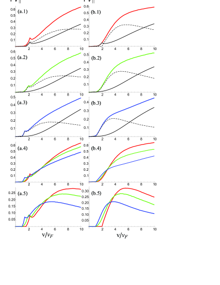
Figure 1: (Color online) Stopping power in units of $(Ze/2\pi)^{2}\epsilon_{s}^{-1}$ as a function of charged particle velocity in units of $v_{F}$. Panels (a) correspond to double layers, panels (b) to single layer configuration. Rows (1), (2) and (3) correspond to $E_{g}/\mu=\left\{{0.0,1.0,1.5}\right\}$, respectively, and are depicted by the red, green and blue curves, correspondingly. The solid black curves are the particle-hole contributions, and the dashed curves represent plasmon contributions. Both (a.4) and (b.4) compare particle hole mode contributions for the three values of the chosen energy gaps, and (a.5) and (b.5) compare the corresponding plasmon contributions.

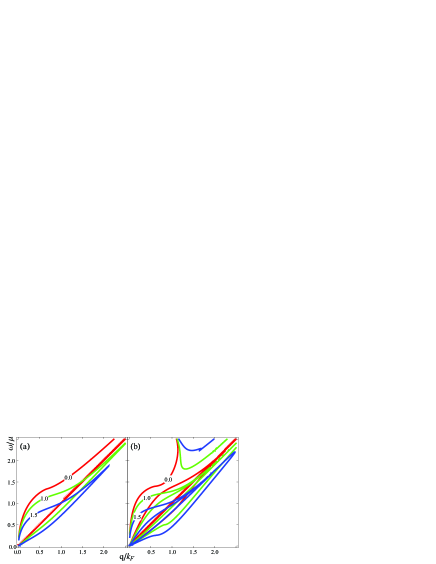
Figure 2: (Color online) Undamped (two higher frequency branches) and damped (two lower in frequency branches) plasmon dispersion relations for gapped graphene. The curves in (a) correspond to a single layer, the curves in (b) to a double layer configuration. The red, green and blue curves show the plasmon dispersion for $E_{g}/\mu=\left\{{0.0,1.0,1.5}\right\}$, respectively.

The simulations shows that the plasmon contribution to the energy loss is decreased with growing $E_{g}$, while the particle-hole contribution remains relatively unaffected by the gap as illustrated by Fig. 1. This may be attributed to diminishing of the plasmon frequency $\omega_{p}(q)\sim\sqrt{q(1-(E_{g}/2\mu)^{2})}$ as shown in Fig. 2 (a). For the double layer configuration, a small spike at low velocity in the plasmon contribution to the energy loss is due to formation of the undamped acoustic (low frequency) and optical (high frequency) plasmon branches. The plasmon modes whose frequency is within the regions

$$\texttt{PH}_{>}=\hbar\omega>\sqrt{h^{2}v^{2}_{F}q^{2}+E^{2}_{g}}$$ (11)

$$\texttt{PH}_{<}=0<\hbar\omega<\mu+\sqrt{\hbar^{2}v_{f}^{2}(q+k_{F})^{2}+(E_{g}/2)^{2}}$$ (12)

are Landau damped and given by $\Re\text{e}\epsilon(q,\omega_{p}-i\gamma)=0$, and also depicted in Fig. 2. The damped plasmons contribute as particle-hole excitations.

The plasmon contribution to the energy loss may be qualitatively explained by spanning the energy loss sector $0<\omega<qv$ through the plasmon dispersion if Fig. 1. In the low velocity regime, given by $\texttt{PH}_{<}(\omega\rightarrow qv)$, one has a contribution from the intraband particle-hole excitations which are relatively weak due to the suppressed backscattering. Once $v$ is increased so that the plasmons start to contribute one has rapid increase in the lost energy. Once the sector fully engulfs the plasmon mode (modes) their contribution reaches its maximum and becomes less than the particle-hole mode contribution when $v/v_{F}\stackrel{{\scriptstyle>}}{{\sim}}8$. After that the increase in the energy loss is governed by the strong interband particle-hole excitations of $\texttt{PH}_{>}$. Both types of the particle-hole excitations are given by the second term in Eq. (10). For gapless graphene the undamped plasmon may live only in the triangular region where the distractive interference between the two types of the particle-hole excitation reduce the imaginary part of the polarization to zero. The gap provides an additional space for the plasmons to run to the higher values of the wave vector. In the double layer configuration both optical and acoustic plasmon modes contribute, but as $v$ is increased, only the optical mode contributes. Since the spectral weight of the acoustical mode is large compared with the optical branch, we see a spike once its contribution reaches the maximum.

The effect of the energy gap on the plasmon contribution to the energy loss is summarized in Figs. 2(a.5) and 2(b.5). These results show intricate interplay between the plasmon and particle-hole contributions to the energy loss, governed by the window in the particle-hole continuum is opened up in the presence of CPEF. On one hand the gap reduces the velocity threshold of the collective plasma excitations. The shorter wave length plasmon frequency become available in the window, and may be accommodated by smaller energy loss sector. Furthermore, the plasmon branch decreases in frequency as $E_{g}$ is increased, as seen in Fig. 2, thereby making it more likely to excite plasmons even when the charged particle speed is low, and making gapped graphene to have a higher stopping power than conventional gapless graphene. On the other hand, the plasmon contribution reaches its maximum for smaller velocities as and the role these collective and particle-hole plasma excitations play in the energy loss are reversed in the high-velocity limit. In this regime where the particle-hole excitations should dominate the window makes the stopping power of gapped graphene being less than when there is no gap.

Appendix A Appendix A

Table 1: Free vs dressed Dirac electron states.

	Free Dirac	Dressed Dirac
Energy	$E_{\mathbf{k}}=\pm k$	$E_{\mathbf{k}}=N_{0}\omega_{0}\pm\sqrt{(E_{g}/2)^{2}+k^{2}}$
Wave	$\left({\begin{array}[]{c}\psi^{+}_{\mathbf{k}}\\ \psi^{-}_{\mathbf{k}}\end{array}}\right)=\frac{\texttt{e}^{i\mathbf{kr}}}{\sqrt{2}}\left({\begin{array}[]{cc}1&\texttt{e}^{i\theta_{\mathbf{k}}}\\ 1&-\texttt{e}^{i\theta_{\mathbf{k}}}\end{array}}\right)\left({\begin{array}[]{c}|{\uparrow}\rangle\\ |{\downarrow}\rangle\end{array}}\right)$	$\left({\begin{array}[]{c}\psi^{+}_{\mathbf{k}}\\ \psi^{-}_{\mathbf{k}}\end{array}}\right)=\frac{\texttt{e}^{i\mathbf{kr}}}{\sqrt{1+\alpha^{2}_{N0,k}}}\left({\begin{array}[]{cc}1&\alpha_{N0,k}\texttt{e}^{i\theta_{\mathbf{k}}}\\ \alpha_{N0,k}&-\texttt{e}^{i\theta_{\mathbf{k}}}\end{array}}\right)\left({\begin{array}[]{c}|{+\frac{1}{2},N_{0}}\rangle\\ |{-\frac{1}{2},N_{0}}\rangle\end{array}}\right)$
Function
Structure	$\mathcal{F}^{\beta}_{\mathbf{k},\mathbf{k+q}}=\frac{1}{2}(1\pm\cos{\theta_{k,k+q}})$	$\begin{array}[]{c}\mathcal{F}^{\beta}_{\mathbf{k},\mathbf{k+q}}=\frac{1}{(1+\alpha^{2}_{N0,k})(1+\alpha^{2}_{N0,k+q})}(1+\alpha^{2}_{N0,k}\alpha^{2}_{N0,k+q}\pm\\ \pm 2\alpha_{N0,k}\alpha_{N0,k+q}\cos{\theta_{k,k+q}}\end{array}$
Factor
Distribution	$f^{\beta}_{k}=\frac{\exp{-\left({E_{\mathbf{k}}-\mu}\right)/k_{B}T}}{1+\exp{-\left({E_{\mathbf{k}}-\mu}\right)/k_{B}T}}$	$f^{\beta}_{k}=\frac{\exp{-\left({E_{\mathbf{k}}-\mu-N_{0}\omega_{0}}\right)/k_{B}T}}{1+\exp{-\left({E_{\mathbf{k}}-\mu-N_{0}\omega_{0}}\right)/k_{B}T}}$
Parameters	$\theta_{k}=\tan^{-1}{\left({\frac{k_{x}}{k_{y}}}\right)}$	$\alpha_{N0,k}=\frac{k}{\sqrt{k^{2}+(E_{g}/2)^{2}}+E_{g}/2}$
	$|{\uparrow}\rangle=\left({\begin{array}[]{c}1\\ 0\end{array}}\right);|{\downarrow}\rangle=\left({\begin{array}[]{c}0\\ 1\end{array}}\right)$	$\left({\begin{array}[]{c}|{+\frac{1}{2}N_{0}}\rangle\\ |{-\frac{1}{2}N_{0}}\rangle\end{array}}\right)=\left({\begin{array}[]{cc}\cos{\left({\frac{\Phi}{2}}\right)}&\sin{\left({\frac{\Phi}{2}}\right)}\\ -\sin{\left({\frac{\Phi}{2}}\right)}&\cos{\left({\frac{\Phi}{2}}\right)}\end{array}}\right)\left({\begin{array}[]{c}|{\uparrow,N_{0}}\rangle\\ |{\downarrow,N_{0}}\rangle\end{array}}\right)$
	$\cos{\theta_{k,k+q}}=\frac{k+q\cos{\theta_{k,q}}}{\sqrt{k^{2}+q^{2}+2kq\cos{\theta_{k,q}}}}$	$\tan^{2}{\left({\frac{\Phi}{2}}\right)}=\frac{\sqrt{\omega^{2}_{0}+4W_{0}^{2}(N_{0}+1)/N_{0}}-\omega_{0}}{\sqrt{\omega^{2}_{0}+4W_{0}^{2}(N_{0}+1)/N_{0}}+\omega_{0}}$

References

- [1] P. R. Wallace, Phys. Rev., 71, 622-634 (1947).
- [2] A. H. C. Neto, F. Guinea, N. M. R. Peres, K. S. Novoselov, and A. K. Geim, Rev. Mod. Phys., 81, 109 (2009).
- [3] D. S. L. Abergel, V. Apalkov, J. Berashevich, K. Ziegler, and T. Chakraborty, Advances in Physics, 59, 261 (2010).
- [4] O. Roslyak, Godfrey Gumbs, and D. H. Huang, Phil. Trans. A 368, 5431-5443 (2010).
- [5] I. Radovic, Lj. Hadzievski, N. Bibic, Z. L. Miskovic, Phys. Rev. A., 76, 042901 (2007).
- [6] I. Radovic, Lj. Hazievski, and Z. L. Miskovic, Phys. Rev. B. 77, 075428 (2008).
- [7] V. Fessatidis, N. J. M. Horing, and A. Balassis, Phys. Lett. A., 375, 192-198, (2010).
- [8] R. H. Ritchie, Phys. Rev., 106, 874 (1957).
- [9] Godfrey Gumbs and N. J. M. Horing, Phys. Rev. B, 43, 2119 (1991).
- [10] N. J. M. Horing, H. C. Tso, and Godfrey Gumbs, Phys. Rev. B., 36, 1588 (1987).
- [11] Godfrey Gumbs and A. Balassis, Phys. Rev. B., 71, 235410 (2005).
- [12] B. Wunsch, T. Stauber, F. Sols, and F. Guinea, New Journal of Physics., 8, 318 (2006).
- [13] O. V. Kibis, Phys. Rev. B., 81, 165433 (2010).
- [14] O. Roslyak, Godfrey Gumbs, and D. Huang, arXiv:1101.5466 ,J. Of. Appl. Phys., (submitted) (2011).
- [15] Xue-Feng Wang and Tapash Chakraborty, Phys. Rev. B, 75, 033408 (2007).
- [16] P. K. Pyatkovskiy, J. Phys.: Condens. Matter, 21, 025506 (2009).
- [17] G. Li, A. Luican, and E.Y. Andrei, Phys. Rev. Lett., 102, 176804 (2009).
- [18] G. Giovannetti, et. al., Phys. Rev. B., 76, 073103, (2007).
- [19] K. W-K. Shung, Phys. Rev. B., 34, 979 (1986).
- [20] K. W-K. Shung, Phys. Rev. B., 34, 1264 (1986).
- [21] G. Gumbs, Sol. State Commun., 65, 393 (1988).
- [22] T.Oka and H.Aoki, Phys. Rev. B., 79, 081406(R) (2009).
- [23] S.V. Syzranov, M.F. Fistul, and K.B. Efetov, Phys. Rev.B., 78, 169901(E) (2008).
- [24] Y. Zhou and M. W. Wu, arXiv:1103.4704v1 (2011).
- [25] H.L. Calvo, H.M. Pastawski, S. Roche and L.E.F. Foa Torres, Appl. Phys. Lett., 98, 232103, (2011).
- [26] M. Grifoni and P. Hanggi, Phys. Rep., 304, 229 (1998).
- [27] S. Kohler, J. Lehmann and P. Hanggi, Phys. Rep., 406, 379 (2005).
- [28] J. Cerne, J. Kono, T. Inoshita, M. Sherwin, M. Sundaram and A.C. Gossard, Appl. Phys. Lett., 70, 3543 (1997).
- [29] K.B. Nordstrom, K. Johensen, S.J. Allen, A.P. Jauho, B. Birnir, J. Kono, T. Noda, H. Akiyama and H. Sakaki, Phys. Rev. Lett., 81, 475 (1998).
- [30] T.Y. Zhang and W. Zhao, Phys. Rev. B., 73, 245337 (2006).
- [31] A. Srivastava, R. Srivastava, J. Wang and J. Kono, Phys. Rev. Lett., 93, 157401 (2004).