Anderson–like Transition for a Class of Random Sparse Models in $d\geq 2$ Dimensions

Abstract

We show that the Kronecker sum of $d\geq 2$ copies of a random one–dimensional sparse model displays a spectral transition of the type predicted by Anderson, from absolutely continuous around the center of the band to pure point around the boundaries. Possible applications to physics and open problems are discussed briefly.

1 Introduction and Summary

In this paper we study a class of models whose relationship to the original Anderson [An] model will now be briefly explained (for further clarification, see section 3). The Anderson Hamiltonian

$$H^{\omega}=\Delta+\lambda V^{\omega}\$$ (1.1)

on

$$l^{2}(\mathbb{Z}^{d})=\left\{u=\left(u_{n}\right)_{n\in\mathbb{Z}^{d}}:u_{n}\in\mathbb{C},\ \sum_{n\in\mathbb{Z}^{d}}\left|u_{n}\right|^{2}<\infty\right\}~{},\qquad d\geq 1,$$

is given by the (centered) discrete Laplacian

$$\left(\Delta u\right)_{n}=\sum_{n^{\prime}:\left|n-n^{\prime}\right|=1}u_{n^{\prime}}$$ (1.2)

plus a perturbation by a random potential

$$\left(V^{\omega}u\right)_{n}=V_{n}^{\omega}u_{n}$$

where $\left\{V_{n}^{\omega}\right\}_{n\in\mathbb{Z}^{d}}$ is a family of independent, identically distributed random variables (i.i.d.r.v.) on the probability space $\left(\Omega,\mathcal{B},\mu\right)$, with a common distribution $F(x)=\mu\left(\left\{\omega:V_{n}^{\omega}\leq x\right\}\right)$; $\lambda>0$ is the disorder parameter also called coupling constant. The spectrum of $H^{\omega}$ is, by the ergodic theorem, almost surely a nonrandom set $\sigma(H^{\omega})=[-2d,2d]+\lambda\text{supp}dF$. Anderson [An] conjectured that there exists a critical coupling constant $0<\lambda_{c}<\infty$ such that for $\lambda\geq\lambda_{c}$ the spectral measure of (1.1) is pure point (p.p) for $\mu$–almost every $\omega$, while, for $\lambda<\lambda_{c}$ the spectral measure of $H^{\omega}$ contains two components, separated by so called “mobility edge” $E^{\pm}$: if $E\in[E^{-},E^{+}]$ the spectrum of $H^{\omega}$ is pure absolutely continuous (a.c); in the complementary set $\sigma(H^{\omega})\backslash[E^{-},E^{+}]$, $H^{\omega}$ has pure point spectra. We refer to [Ji] for a comprehensive review on the status of the problem and references, and only wish to remark that for $d=1$ the spectrum is p.p. for all $\lambda$ for almost every $\omega$ ([GMP, KS]), while, for $d\geq 2$ the existence of a.c. spectrum is open, except for the version of (1.1) on the Bethe lattice, where it was first proved by A. Klein in a seminal paper [Kl] (see also [Ji], Section 2.31).

Given the above mentioned difficulties, one might be led to study the limit $\lambda\rightarrow 0$ of (1.1), for which the spectrum is pure a.c.. We shall instead follow a different approach to the Anderson conjecture suggested by Molchanov: the limit of zero concentration, i.e., taking $V^{\omega}$ in (1.1) such that

$$V_{n}^{\omega}=\sum_{i}\varphi_{i}^{\omega}(n-a_{i})~{},$$ (1.3)

with elementary potential (“bump”) $\varphi^{\omega}:\mathbb{Z}^{d}\longrightarrow\mathbb{R}$ satisfying a uniform integrability condition

$$\left|\varphi^{\omega}(z)\right|\leq\frac{C_{0}}{1+\left|z\right|^{d+\varepsilon}}$$ (1.4)

for some $\varepsilon>0$ and $0<C_{0}<\infty$ and

$$\lim_{R\rightarrow\infty}\frac{\#\left\{i:\left|a_{i}\right|\leq R\right\}}{R^{d}}=0\ .$$ (1.5)

Due to condition (1.5) of zero concentration, potentials such as (1.3) are called sparse and have been intensively studied in recent years since the seminal work by Pearson in dimension $d=1$ [Pe], notably by Kiselev, Last and Simon [KLS] for $d=1$ and by Molchanov in the multidimensional case [Mo1] (see also [MoV, Mo2] for complete proofs and additional results). As a consequence of (1.4), for $d\geq 2$ the interaction between bumps is weak [Mo1] while for $d=1$ the phase of the wave after propagation between distant bumps become “stochastic” [Pe]. This is the right moment to introduce our one–dimensional model.

Instead of (1.1) we shall adopt an off–diagonal Hamiltonian which contains the Laplacian (1.2):

$$J^{\omega}\equiv J_{P^{\omega}}=\left(\begin{array}[]{ccccc}0&p_{0}&0&0&\cdots\\ p_{0}&0&p_{1}&0&\cdots\\ 0&p_{1}&0&p_{2}&\cdots\\ 0&0&p_{2}&0&\cdots\\ \vdots&\vdots&\vdots&\vdots&\ddots\end{array}\right)\;,$$ (1.6)

for each sequence $P^{\omega}=(p_{n}^{\omega})_{n\geq 0}$ of the form

$$p_{n}^{\omega}=\left\{\begin{array}[]{lll}p&\mathrm{if}&n=a_{j}^{\omega}~{}\text{for some }j\\ 1&\mathrm{if}&\text{otherwise}\,,\end{array}\right.$$ (1.7)

for $p\in(0,1)$. Above, $\{a_{j}^{\omega}\}_{j\geq 1}$ is a random set of natural numbers

$$a_{j}^{\omega}=a_{j}+\omega_{j}$$

with $a_{j}$ satisfying the “sparseness” condition

$$a_{j}-a_{j-1}=\beta^{j}\;,\qquad\qquad j=2,3,\ldots$$ (1.8)

with $a_{1}+1=\beta\geq 2$ where $\beta$ is an integer and $\omega_{j}$, $j\geq 1$, are independent random variables defined on a probability space $(\Omega,\mathcal{B},\nu)$, uniformly distributed on the set $\Lambda_{j}=\{-j,\ldots,j\}$. We denote by $J_{\phi}^{\omega}$ an operator related to the Jacobi matrix $J^{\omega}$ acting on the Hilbert space $\mathcal{H}$ of square summable complex valued sequences $u=\left(u_{n}\right)_{n\geq-1}$ satisfying a $\phi$-boundary condition at $-1$:

$$\left(J_{\phi}^{\omega}u\right)_{n}=p_{n-1}^{\omega}u_{n-1}+p_{n}u_{n+1}$$ (1.9)

for $n\geq 0$, with $p_{-1}^{\omega}=1$ and

$$u_{-1}\cos\phi-u_{0}\sin\phi=0$$ (1.10)

(i.e., $\left(J_{\phi}^{\omega}u\right)_{n}=\left(J_{0}^{\omega}u\right)_{n}+\delta_{0,n}\tan\phi~{}u_{0}$). The variables $\left\{\omega_{j}\right\}_{j\geq 1}$ introduce uncertainty in the positions $\{a_{j}\}_{j\geq 1}$ where the “bumps” are located. The corresponding diagonal version satisfies trivially (1.4), since $\varphi_{i}^{\omega}(n)=\delta_{\omega_{i},n}$ is just a Kronecker delta at $\omega_{i}$; such models are nowadays called Poisson models (see pg. 624 of [Ji] and references therein). A disordered diagonal model of the above type- to which our results are also applicable- was introduced by Zlatoš [Zl]. The present non–diagonal version has some advantages in addition to the initial motivation coming from [H1]: that the spectrum $\sigma(J^{\omega})$ of $J^{\omega}$ interpolates between purely absolutely continuous for $p=1$ and dense pure point for $p=0$ (in the latter case, $J^{\omega}$ is a direct sum of finite matrices; the dense character is due to (1.8)). It is easily proved that the essential spectrum of $J^{\omega}$ is $\sigma_{\mathrm{ess}}(J^{\omega})=[-2,2]$ (see [CMW1]).

We may ask whether the p.p. part of $\sigma(J^{\omega})$ for $p=0$ above persists in some nonempty interval. Let

$$I=\left\{\lambda\in[-2,2]:v^{-2}(\beta-1)(4-\lambda^{2})\geq 1\right\}$$ (1.11)

where $v=v(p)=(1-p^{2})/p$ and set

$$I^{c}=[-2,2]\backslash I~{}.$$ (1.12)

Note that $I=\emptyset$ (consequently, $I^{c}=\left[-2,2\right]$) if $p<p_{c}$, where $p_{c}$ is defined by

$$v^{2}(p_{c})=\left(\frac{1-p_{c}^{2}}{p_{c}}\right)^{2}=4(\beta-1)~{}.$$

Such a equation has always a solution $p_{c}=\sqrt{2\beta-1-2\sqrt{\beta^{2}-\beta}}$ in $\left(0,1\right)$ for $\beta\geq 2$ and $v_{c}=v(p_{c})=2\sqrt{\beta-1}$ will play a role similar to the critical coupling $\lambda_{c}$ of the Anderson model. We have (see Theorem 2.4 of [CMW1])

Theorem 1.1

Let $J_{\phi}^{\omega}$ be defined by (1.6)–(1.10), and set

$$A_{\mathrm{sc}} = 2\cos\pi\mathbb{Q}\cap I$$

$$A_{\mathrm{pp}} = 2\cos\pi\mathbb{Q}\cap I^{c}~{}.$$ (1.13)

Then, for $\nu$–almost every $\omega$,

1. the spectrum of $J_{\phi}^{\omega}$ restricted to the set $I\backslash A_{\mathrm{sc}}^{\prime}$ with $A_{\mathrm{sc}}^{\prime}=A_{\mathrm{sc}}\cup A^{\prime}$ and $A^{\prime}$ a set of Lebesgue measure zero, is purely singular continuous;

2. the spectrum of $J_{\phi}^{\omega}$ is dense pure point when restricted to $I^{c}\backslash A_{\mathrm{pp}}$ for almost every $\phi\in[0,\pi)$.

Remark 1.2

1. The occurrence of the set $A^{\prime}$ of Lebesgue measure zero is related to the definition of essential (or minimal) support of the spectral measure $\mu$ (see Definition 1 of [GP])).

2. As we have excluded a countable set $A_{pp}$, the spectrum is purely p.p. in $I^{c}$.

Theorem 1.1 for the corresponding diagonal model was proved in [Zl], except for the specification of the set $A_{pp}$, which leads to the refinement of Remark 1.2.2. The latter depended on the details of the method in [CMW1], whose crucial step was a proof that the sequence of Prüfer angles $\left(\theta_{j}^{\omega}\right)_{j\geq 0}$ (see [KLS, Zl, MWGA] for definitions) is uniformly distributed mod $\pi$ (u.d. mod $\pi$) for $\nu$–almost every $\omega$ and for all $\lambda=2\cos\varphi$ with $\varphi\in[0,\pi]$ such that $\varphi/\pi$ is an irrational number. As remarked by Remling [Re] in his review of [MWGA], which introduced our method, the new idea was to fix the energy $\lambda$ and assume (or prove, when one is able to) that the Prüfer angles $\left(\theta_{j}^{\omega}\right)$ at $a_{j}$ are uniformly distributed (u.d.) as a function of $j$, instead of the traditional approach which exploits the u.d. of the Prüfer angles in the energy variable at fixed $a_{j}$. We shall see that this refinement, perhaps of apparently minor importance, will play an important role in our approach (see Remark 2.9). Figure 1 depicts the one–dimensional spectral transition, where the “mobility edges” $\lambda^{\pm}=2\cos\varphi^{\pm}$ are implicitly given by the equation

$$1-\frac{\lambda^{2}}{4}=\sin^{2}\varphi=\frac{v^{2}}{v_{c}^{2}}$$

provided $v<v_{c}=2\sqrt{\beta-1}$.

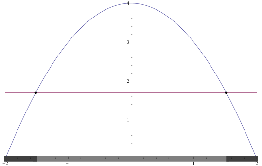
Figure 1: Singular continuous (light gray) and pure point (dark gray) spectra separated by the “mobility edges” $\lambda^{\pm}=\pm 2\sqrt{1-v^{2}/v^{2}_{c}}$; $v/v_{c}=1.3038...$

For superexponential sparseness, i.e., $a_{j}-a_{j-1}=\left[e^{cn^{\gamma}}\right]$ ($\left[z\right]$ the integer part of $z$), with $c>0$, $\gamma>1$ and $\left\{\omega_{j}\right\}_{j\geq 1}$ independent random variable, uniform in $\Lambda_{j}$, it may be proved that $\sigma(J_{\phi}^{\omega})$ is purely singular continuous (s.c.) for almost every $\omega\in\times_{j=1}^{\infty}$ $\{-j,\ldots,j\}$ ([CMW1], Theorem 5.2). This has a simple physical interpretation already pointed out by Pearson [Pe]: the enormous separation between the $a_{j}$ causes the aforementioned “stochasticity” of the phase of the Bloch wave of difference Laplacian , with the particle behaving as if successively undergoing reflections (and transmissions) through the bumps. The reflection from the latter is $O\left(v^{2}\right)$ by the Born approximation, and, since $\displaystyle\sum_{n\geq 0}(1-p_{n}^{2})^{2}/p_{n}^{2}=\infty$, no particles arrive at infinity (for $\displaystyle\sum_{n\geq 0}(1-p_{n}^{2})^{2}/p_{n}^{2}<\infty$, the spectrum is purely a.c. as may be proved by methods of [KLS]). This conclusion is rigorously confirmed by the dynamics: the average time spent by the particle, in any bounded region, is zero for states both in the a.c. and s.c. subspaces, by the RAGE theorem [RS2], but the “sojourn time” (properly defined, see [Si]) for a particle in the s.c. subspace has, in contrast to the a.c. case, to be infinite for some finite region of space as a consequence of Theorem 1 of [Si].

On the other hand, for subexponential sparseness, with $a_{j}-a_{j-1}=\left[e^{cn^{\gamma}}\right]$ with $\gamma<1$ and everything else as before, $\sigma_{\mathrm{ess}}(J_{\phi}^{\omega})=\sigma_{\mathrm{pp}}(J_{\phi}^{\omega})=\left[-2,2\right]$ for a.e. boundary phase $\phi\in\left[0,\pi\right]$ and for a.e. $\omega\in\times_{j=1}^{\infty}$ $\{-j,\ldots,j\}$ ([CMW1], Theorem 5.1).

These results joins smoothly to the one (corresponding to $\gamma=0$) for the standard Anderson model in $d=1$, according to which all states are localized [GMP, KS]. The latter is believed to be physically related to the subtle instability of tunneling [JMS, S1] which is strongest in $d=1$.

What is really surprising in Theorem 1.1 is, of course, not the existence of s.c. spectrum, but that of p.p. spectrum in a regime of high (exponential) sparsity (1.8). That is the more so because the well–known instability of Anderson localization under rank one perturbations [dR] implies that the spectral measure associated to s.c. spectrum which is obtained in the Anderson model by changing the value of the potential at a point is supported on a set of zero Hausdorff dimension, which is not the case for $J_{\phi}^{\omega}$ (see [Zl, CMW2]). Thus the spectral transition depicted in the latter is of the robust type. For further general references on random systems, see [CL], [PF], [Sto].

We now summarize the contents of the paper. In Section 2 we prove our main result (Theorem 2.6), which states that the Kronecker sum of $d\geq 2$ copies of $J_{\phi}^{\omega}$ exhibits a Anderson transition (see also Section 3 for this designation and a discussion of possible application to the Anderson transition in lightly-doped semiconductors) from a.c. spectrum for small energy (i.e., in the region situated around the center of the band) to dense p.p. for large energy (i.e., in the union of the two regions around the extreme points): this is true for suitable values of parameters, and exclusion of resonances.

The proof of our main result (Theorem 2.6) shows that ideas of Kahane and Salem [KS1, KS2] combine with the Strichartz-Last theorem [Str, L1] in a neat way, yielding a result of quite general nature, i.e., showing the existence of a.c. spectrum for any Kronecker sum of operators $A\otimes I+\theta I\otimes A$ for a.e. $\theta\in[0,1]$ whenever $A$ has s.c. spectrum in some nonempty interval with local Hausdorff dimension greater than $1/2$. For this reason, we believe that the idea might have further potential applications, e.g., to the intermediate region, see the discussion in Section 3. For a physically related model - the Anderson random potential on tree graphs (i.e. Bethe lattice) at weak disorder, absence of mobility edge has been shown recently [AW1]. We also refer to [AW2] for the important proof of existence of a.c. spectra in quantum tree graphs with weak disorder, as well as [AW1] for further literature on quantum tree graphs.

2 Main Result

In order to formulate and prove our main result (Theorem 2.6) we need the following [Zl]:

Definition 2.1

A finite Borel measure $\mu$ has exact local Hausdorff dimension $\alpha(\cdot)$ in an interval $I$ if for any $\lambda\in I$ there exists an $\alpha(\lambda)$ such that for any $\varepsilon>0$ there is a $\delta>0$ with $\mu\left((\lambda-\delta,\lambda+\delta)\cap\cdot\right)$ is both $(\alpha(\lambda)-\varepsilon)$–continuous and $(\alpha(\lambda)+\varepsilon)$–singular.

The above notion of continuous and singular refer to the Hausdorff measure $h^{\alpha}$ (see e.g. Section 4 of [L1] for a convenient summary of all relevant concepts and references).

Definition 2.2 (Definition 2.1 of [L1])

We say that $\mu$ is uniformly $\alpha$–Hölder continuous (U$\alpha$H) iff there exists a constant $C$ such that, for every interval $I$ with $\left|I\right|<1$,

$$\mu\left(I\right)<C\left|I\right|^{\alpha}$$

Above, $\left|S\right|$ denotes Lebesgue measure of $S$. Let $\left\{E(\lambda)\right\}$ denote the spectral family associated to $J_{\phi}^{\omega}$ (we omit the indices for simplicity) and $\left\{E_{\mathrm{sc}}(\lambda)\right\}$, $\left\{E_{\mathrm{pp}}(\lambda)\right\}$ its singular continuous and pure point parts. As usual (see e.g. [KS]), we define $\mathcal{H}_{\mathrm{sc}}$ and $\mathcal{H}_{\mathrm{pp}}$ so that, if $\psi\in\mathcal{H}_{sc}$ the spectral measure,

$$\mu_{\psi}^{\mathrm{sc}}(\lambda)\equiv\left(\psi,E(\lambda)\psi\right)~{},$$ (2.1a)

is purely singular continuous and, if $$\psi\in\mathcal{H}_{\mathrm{pp}}$$,

$$\ \mu_{\psi}^{\mathrm{pp}}(\lambda)\equiv\left(\psi,E(\lambda)\psi\right)~{},$$ (2.1b)

is purely pure point. $$\mathcal{H}_{\mathrm{sc}} \mathcal{H}_{\mathrm{pp}} \mathcal{H=H}_{\mathrm{sc}}\oplus\mathcal{H}_{\mathrm{pp}} J_{\phi}^{\omega}$$ and are closed (in norm), mutually orthogonal subspaces: , and invariant under .

By [Zl, CMW2] the local Hausdorff dimension (Definition 2.1) associated to $J_{\phi}^{\omega}\upharpoonright I$, with $I$ given by (1.11), is

$$\alpha(\lambda)=1-\frac{\log r(\lambda)}{\log\beta}$$ (2.2)

where

$$r(\lambda)=1+\frac{v^{2}}{4-\lambda^{2}}~{}.$$ (2.3)

We now choose an arbitrary $\varepsilon>0$ and pick $\left(\lambda_{i}\right)_{i=1}^{N_{\varepsilon}}$ with $\lambda_{i}\in I$ and $\left(\delta_{\varepsilon}^{i}\right)_{i=1}^{N_{\varepsilon}}$, with

$$0<\delta_{\varepsilon}^{i}<1~{},$$ (2.4a)

for some $$N_{\varepsilon}<\infty$$, in such way that

$$\lambda_{1}-\delta_{\varepsilon}^{1} = -\sqrt{4-v^{2}/(\beta-1)}~{},$$ (2.4b)

$$\lambda_{i}+\delta_{\varepsilon}^{i} = \lambda_{i+1}-\delta_{\varepsilon}^{i+1}\ ,\quad i=1,\ldots,N_{\varepsilon}-1~{},$$ (2.4c)

$$\lambda_{N_{\varepsilon}}+\delta_{\varepsilon}^{N_{\varepsilon}} = \sqrt{4-v^{2}/(\beta-1)}~{}.$$ (2.4d)

We set

$$A_{\varepsilon}^{i}=[\lambda_{i}-\delta_{\varepsilon}^{i},\lambda_{i}+\delta_{\varepsilon}^{i})~{},$$ (2.4e)

for $$1\leq i<N_{\varepsilon} A_{\varepsilon}^{N_{\varepsilon}}=[\lambda_{N_{\varepsilon}}-\delta_{\varepsilon}^{N_{\varepsilon}},\lambda_{N_{\varepsilon}}+\delta_{\varepsilon}^{N_{\varepsilon}}]$$, with , and

$$~{}\tilde{A}_{\varepsilon}^{i}=(\lambda_{i}-\delta_{\varepsilon}^{i},\lambda_{i}+\delta_{\varepsilon}^{i})~{},$$ (2.4f)

for $$1\leq i\leq N_{\varepsilon} I$$, and write as a mutually disjoint union:

$$I=\bigcup_{i=1}^{N_{\varepsilon}}A_{\varepsilon}^{i}~{}.$$ (2.5)

Observe that (2.4b) and (2.4d) represent the boundary points $\lambda_{\pm}$ of $I$, given by (1.11). The choice of $\left(\lambda_{i}\right)_{i=1}^{N_{\varepsilon}}$ is arbitrary but the quantities $\delta_{\varepsilon}^{i}$, $i=1,\ldots,N_{\varepsilon}$, are chosen in correspondence to $\varepsilon$ according to Definition 2.1, with $\alpha(\cdot)$ given by (2.2), and satisfy

$$\bar{\delta}_{\varepsilon}\equiv\max_{i}\delta_{\varepsilon}^{i}\rightarrow 0~{},$$ (2.6)

by continuity, as $\varepsilon$ tends to $0$. As a consequence, the spectral measure of $J_{\phi}^{\omega}$ restricted to $\tilde{A}_{\varepsilon}^{i}$

$$\mu_{\psi}^{\mathrm{sc}}\upharpoonright\tilde{A}_{\varepsilon}^{i}$$ (2.7)

is $\left(\alpha(\lambda_{i})-\varepsilon\right)$–continuous and $\left(\alpha(\lambda_{i})+\varepsilon\right)$–singular, for $i=1,\ldots,N_{\varepsilon}$.

Proposition 2.3

Under the hypotheses of Theorem 1.1 and (2.2)–(2.7), there exists a dense set $D$ in $\mathcal{H}_{\mathrm{sc}}$ such that, $\forall\psi\in D$, $\mu_{\psi}^{\mathrm{sc}}\upharpoonright\tilde{A}_{\varepsilon}^{i}$ is, for each $i\in\left\{1,,\ldots,N_{\varepsilon}\right\}$, uniformly $\left(\alpha(\lambda_{i})-\varepsilon\right)$–Hölder continuous.

Proof. We write

$$\mathcal{H}=\displaystyle\bigoplus_{i=1}^{N_{\varepsilon}}\mathcal{H}_{i}$$

where $\mathcal{H}_{i}$ is the subspace of $\mathcal{H}_{\mathrm{sc}}$ generated by

$$\left\{E_{I}\psi:\psi\in\mathcal{H}_{\mathrm{sc}}~{},\ \text{for every }I=(\lambda,\lambda^{\prime}]\subset\tilde{A}_{\varepsilon}^{i}\right\}$$

where $E_{I}=\displaystyle\int_{I}dE(\lambda)$ is the spectral projection on $I$. By (2.2)–(2.7) and Theorem 5.2 of [L1], for each $\mathcal{H}_{i}$ we may choose $D_{i}$ dense in $\mathcal{H}_{i}$ such that, $\forall\psi\in D_{i}$, $\mu_{\psi}$ is uniformly $\left(\alpha(\lambda_{i})-\varepsilon\right)$–Hölder continuous. Since the subspace $\mathcal{M}$ generated by $\left\{E(\lambda_{i}+\delta_{\varepsilon}^{i})\psi:\psi\in\mathcal{H}\right\}$ for $i=1,\ldots,N_{\varepsilon}-1$ is such that $\mathcal{M}\subset\mathcal{H}_{\mathrm{sc}}^{\bot}$, we have by (2.4c), (2.4e) and (2.5) that $\bigoplus_{i=1}^{N_{\varepsilon}}D_{i}$ is dense in $\mathcal{H}_{\mathrm{sc}}$ and satisfies the assertion by (2.7).

$\Box$

Corollary 2.4

Let $I_{0}\subseteq I$ and $\psi\in D$. Then $\mu_{\psi}^{\mathrm{sc}}\upharpoonright I_{0}$ is U$\alpha$H, where

$$\alpha=\min_{i:\tilde{A}_{\varepsilon}^{i}\cap I_{0}\neq\emptyset}\alpha(\lambda_{i})-\varepsilon~{}.$$ (2.8)

Proof. This follows immediately from Proposition 2.3, Definition 2.2 and additivity of $\mu_{\psi}^{\mathrm{sc}}$.

$\Box$

In the rest of the paper we assume that $\varepsilon$ and $\left(\delta_{\varepsilon}^{i}\right)_{i=1}^{N_{\varepsilon}}$ is a given fixed set of numbers, with $\varepsilon>0$ arbitrarily small (but with $N_{\varepsilon}<\infty$). Consider the Kronecker sum of two copies of $J_{\phi}^{\omega}$ as an operator on $\mathcal{H}\otimes\mathcal{H}$:

$$J_{\theta}^{(2)}:=J_{\phi}^{\omega^{1}}\otimes I+\theta I\otimes J_{\phi}^{\omega^{2}}$$ (2.9)

where $\omega^{1}=\left(\omega_{j}^{1}\right)_{j\geq 1}$ and $\omega^{2}=\left(\omega_{j}^{2}\right)_{j\geq 1}$ are two independent sequences of independent random variables defined in $\left(\Omega,\mathcal{B},\nu\right)$, as before (we omit $\omega^{1}$ and $\omega^{2}$ in the l.h.s. of (2.9) for brevity). Above, the parameter $\theta\in[0,1]$ is included to avoid resonances (see Remark 2.10). We ask for properties of $J_{\theta}^{(2)}$ (e.g. the spectral type) which hold for typical configurations, i.e., a.e. $\left(\omega^{1},\omega^{2},\theta\right)$ with respect to $\nu\times\nu\times l$ where $l$ is the Lebesgue measure in $[0,1]$. $J_{\theta}^{(2)}$ is a special two–dimensional analog of $J_{\phi}^{\omega}$; if the latter was replaced by $-\Delta+V$ on $L^{2}(\mathbb{R},dx)$ where $\Delta=d^{2}/dx^{2}$ is the second derivative operator, and $V$ a multiplicative operator $V\psi(x)=V(x)\psi(x)$ (potential), the sum (2.9) would correspond to $\left(-d^{2}/dx_{1}^{2}+V_{1}\right)+\left(-d^{2}/dx_{2}^{2}+V_{2}\right)$ on $L^{2}(\mathbb{R}^{2},dx_{1}dx_{2})$, i.e., the “separable case” in two dimensions. Accordingly, we shall also refer to $J_{\theta}^{(n)}$, $n=2,3,\ldots$, as the separable case in $n$ dimensions.

Our approach is to look at the quantity

$$\left(\Phi,e^{-itJ_{\theta}^{(2)}}\Psi\right)=f^{1}(t)f^{2}(\theta t)$$ (2.10a)

by (2.9), where

$$f^{i}(s)=f_{\mathrm{sc}}^{i}(s)+f_{\mathrm{pp}}^{i}(s)~{},\quad i=1,2$$ (2.10b)

with

$$f_{\mathrm{sc}}^{i}(s) = \int e^{-is\lambda}d\mu_{\varphi_{i},\psi_{i}}^{\mathrm{sc}}(\lambda)$$ (2.10c)

$$f_{\mathrm{pp}}^{i}(s) = \int e^{-is\lambda}d\mu_{\rho_{i},\chi_{i}}^{\mathrm{pp}}(\lambda)$$ (2.10d)

Above $$\Phi,\Psi\in\mathcal{H}\otimes\mathcal{H}$$,

$$\Phi = \left(\varphi_{1}\dot{+}\rho_{1}\right)\otimes\left(\varphi_{2}\dot{+}\rho_{2}\right)~{},$$ (2.11a)

$$\Psi = \left(\psi_{1}\dot{+}\chi_{1}\right)\otimes\left(\psi_{2}\dot{+}\chi_{2}\right)~{},$$ (2.11b)

with $$\varphi_{i},\psi_{i}\in\mathcal{H}_{\mathrm{sc}} \rho_{i},\chi_{i}\in\mathcal{H}_{\mathrm{pp}} \varphi\dot{+}\rho \varphi,\rho\in\mathcal{H}$$, and denotes the direct sum of two vectors . The vectors

$$\varphi_{1},\psi_{1}\in D_{1}\ ,\quad\varphi_{2},\psi_{2}\in D_{2}$$ (2.11c)

where $$D_{1} D_{2} D \varphi_{i}\dot{+}\rho_{i},~{}\psi_{i}\dot{+}\chi_{i} \mathcal{H}= \mathcal{H}_{\mathrm{sc}}\oplus\mathcal{H}_{\mathrm{pp}} \mu_{\varphi,\psi}^{\mathrm{sc}}(\lambda)=\left(\varphi,E(\lambda)\psi\right) \mu_{\rho,\chi}^{\mathrm{pp}}(\lambda)=\left(\rho,E(\lambda)\chi\right) f$$ and are copies of the set occurring in Proposition 2.3; by (2.11a), (2.11b) and (2.11c), run through a dense set in . In (2.10c) and (2.10d), , as in (2.1a) and (2.1b), the ’s being the corresponding Fourier–Stieltjes (F.S.) transforms. By (2.10a) and (2.10b)

$$\left(\Phi,e^{-itJ_{\theta}^{(2)}}\Psi\right)=g(t,\theta)+h(t,\theta)+k(t,\theta)$$ (2.12a)

where

$$g(t,\theta) = f_{\mathrm{sc}}^{1}(t)f_{\mathrm{sc}}^{2}(\theta t)$$ (2.12b)

$$h(t,\theta) = f_{\mathrm{sc}}^{1}(t)f_{\mathrm{pp}}^{2}(\theta t)+f_{\mathrm{pp}}^{1}(t)f_{\mathrm{sc}}^{2}(\theta t)$$ (2.12c)

$$k(t,\theta) = f_{\mathrm{pp}}^{1}(t)f_{\mathrm{pp}}^{2}(\theta t)$$ (2.12d)

are the F.S. transforms of the complex valued spectral measures of $$J_{\theta}^{(2)} \mathcal{H}_{\mathrm{sc}}\oplus\mathcal{H}_{\mathrm{sc}} \mathcal{H}_{\mathrm{sc}}\oplus\mathcal{H}_{\mathrm{pp}}\cup\mathcal{H}_{\mathrm{pp}}\oplus\mathcal{H}_{\mathrm{sc}} \mathcal{H}_{\mathrm{pp}}\oplus\mathcal{H}_{\mathrm{pp}} g \mu_{\varphi_{1}}^{\mathrm{sc}} \tilde{\mu}_{\varphi_{2}}^{\mathrm{sc}}$$ associated with , and , respectively. It follows from (2.12b) that is F.S. transform of the convolution of the measures and with

$$\tilde{\mu}_{\varphi_{2}}^{\mathrm{sc}}(\lambda)\equiv\mu_{\varphi_{2}}^{\mathrm{sc}}(\lambda/\theta)~{},\qquad\theta\neq 0$$ (2.13)

defined by (see [Kat], pg. 41):

$$\mu_{\varphi_{1}}^{\mathrm{sc}}\ast\tilde{\mu}_{\varphi_{2}}^{\mathrm{sc}}(B)=\int\mu_{\varphi_{1}}^{\mathrm{sc}}(B-\lambda)d\tilde{\mu}_{\varphi_{2}}^{\mathrm{sc}}(\lambda)$$ (2.14)

for any Borel set $B$ of $\mathbb{R}$, where $B-\lambda\equiv B-\left\{\lambda\right\}=\left\{x-\lambda:x\in B\right\}$, and analogously for $h$ and $k$.

At least since the paper of Kahane and Salem [KS1] of 1958, it is well known that the convolution of two s.c. measures may be absolutely continuous (this possibility was revived for models in mathematical physics by [MM]). Their proof, as well as our proof of the corresponding assertion in the forthcoming Theorem 2.6, was based on the following folklore proposition:

Proposition 2.5

Let $\mu$ be a measure on the space $M(\mathbb{R})$ of all finite regular Borel measures on $\mathbb{R}$. If the Fourier–Stieltjes transform of $\mu$

$$\mathbb{R}\ni t\longmapsto\hat{\mu}(t)=\int e^{-it\lambda}d\mu(\lambda)$$ (2.15)

belongs to $L^{2}(\mathbb{R},dt)$, then $\mu$ is absolutely continuous with respect to Lebesgue measure.

Proof See ([C], exercise 11, pg. 159) or [Si]; for a generalization of this result using different methods, see [Es].

We now go back to Theorem 1.1. Let

$$\lambda^{\pm}=\pm 2\sqrt{1-\frac{v^{2}}{v_{c}^{2}}}$$ (2.16)

under the condition

$$0<v<v_{c}=2\sqrt{\beta-1}$$ (2.17)

so that

$$0<\lambda^{+}<2~{}.$$ (2.18)

We are now ready to state our main result:

Theorem 2.6

Let $J_{\theta}^{(2)}$ be defined by (2.9) and let

$$v^{2}<a\left(\sqrt{\beta}-1\right)<v_{c}^{2}~{}$$ (2.19)

with $a<4$. Then, for almost every $\left(\omega^{1},\omega^{2},\theta\right)$ with respect to $\nu\times\nu\times l$,

1. there exist $\tilde{\lambda}^{\pm}$ with $\tilde{\lambda}^{+}=-\tilde{\lambda}^{-}$ and

   $$0<\tilde{\lambda}^{+}<\lambda^{+}$$ (2.20a)

   such that

   $$\left(\tilde{\lambda}^{-}(1+\theta),\tilde{\lambda}^{+}(1+\theta)\right)\subset\sigma_{\mathrm{ac}}\left(J_{\theta}^{(2)}\right)$$ (2.20b)

2. $$\left[-2(1+\theta),\lambda^{-}(1+\theta)\right)\cup\left(\lambda^{+}(1+\theta),2(1+\theta)\right]\subset\sigma_{\mathrm{pp}}\left(J_{\theta}^{(2)}\right)$$ (2.20c)

3. $$\sigma_{\mathrm{sc}}\left(J_{\theta}^{(2)}\right)\cap\left(\lambda^{-}(1+\theta),\lambda^{+}(1+\theta)\right)$$ (2.20d)

   may, or may not, be an empty set.

Proof. We first choose $I_{0}$ in Corollary 2.4 such that

$$I_{0}=\left[-\tilde{\lambda}^{+},\tilde{\lambda}^{+}\right]$$ (2.21)

and

$$\alpha=\min_{i:\tilde{A}_{\varepsilon}^{i}\cap I_{0}\neq\emptyset}\alpha(\lambda_{i})-\varepsilon>\frac{1}{2}~{}.$$ (2.22)

The inequalities (2.20a) and (2.22) are established in Appendix A (Proposition A.1) for any choice of parameters $p$, $\beta$ satisfying (2.19) and $\varepsilon$ depending on $p$, $\beta$ and $a$.

Coming back to (2.10c), by polarization we need only consider $\varphi_{1}=\psi_{1}\in D_{1}$, $\varphi_{2}=\psi_{2}\in D_{2}$ and, accordingly, with (2.21) and (2.22), we define

$$f_{\mathrm{sc}}^{i}(s):=\int_{I_{0}}e^{-is\lambda}d\mu_{\varphi_{i}}^{\mathrm{sc}}(\lambda)~{},\qquad i=1,2$$ (2.23)

in (2.12a).

Let

$$I_{i}(T):=\int_{0}^{T}\left|f_{\mathrm{sc}}^{i}(s)\right|^{2}ds$$ (2.24)

By Strichartz’ theorem [Str] (see also Theorem 2.5 of [L1], for a slick proof) and (2.21)

$$I_{i}(T)\leq C_{i}T^{1-\alpha}\leq CT^{1-\alpha}$$ (2.25)

for $0<C_{i}<\infty$, $i=1,2$, $T$–independent constants and $C=\max(C_{1},C_{2})$. By (2.23) and (2.25) and a change of variable, we have

$$\int_{0}^{1}\left|f_{\mathrm{sc}}^{2}(\theta t)\right|^{2}d\theta=\frac{1}{t}I_{2}(t)\leq Ct^{-\alpha}~{}$$

which implies

$$\int_{1}^{T}dt\left|f_{\mathrm{sc}}^{1}(t)\right|^{2}\int_{0}^{1}\left|f_{\mathrm{sc}}^{2}(\theta t)\right|^{2}d\theta\leq C\int_{1}^{T}\left|f_{\mathrm{sc}}^{1}(t)\right|^{2}t^{-\alpha}dt~{}.$$ (2.26)

We now perform an integration by parts on the r.h.s. of (2.26)

$$\int_{1}^{T}\left|f_{\mathrm{sc}}^{1}(t)\right|^{2}t^{-\alpha}dt=\left.I_{1}(t)t^{-\alpha}\right|_{1}^{T}+\alpha\int_{1}^{T}dtI_{1}(t)t^{-\alpha-1}$$ (2.27)

By (2.26), (2.27) and Fubini’s theorem ($T\geq 1$)

$$\int_{0}^{1}d\theta\int_{1}^{T}\left|f_{\mathrm{sc}}^{1}(t)\right|^{2}\left|f_{\mathrm{sc}}^{2}(\theta t)\right|^{2}dt \leq CT^{1-2\alpha}+\alpha C\int_{1}^{T}dtt^{-2\alpha}$$ (2.28)

$$\leq C\frac{1}{2\alpha-1}\left(\alpha-(1-\alpha)T^{1-2\alpha}\right)~{}.$$

By (2.22) and (2.28), the limit

$$\int_{0}^{1}d\theta\int_{0}^{\infty}\left|f_{\mathrm{sc}}^{1}(t)\right|^{2}\left|f_{\mathrm{sc}}^{2}(\theta t)\right|^{2}dt=\lim_{T\rightarrow\infty}\int_{0}^{1}d\theta\int_{0}^{T}\left|f_{\mathrm{sc}}^{1}(t)\right|^{2}\left|f_{\mathrm{sc}}^{2}(\theta t)\right|^{2}dt~{}$$

exists, is finite and

$$\int_{0}^{\infty}\left|f_{\mathrm{sc}}^{1}(t)\right|^{2}\left|f_{\mathrm{sc}}^{2}(\theta t)\right|^{2}dt<\infty$$ (2.29)

for a.e. $\theta\in\left[0,1\right]$. By Ichinose’s theorem [I] (actually, Theorem VIII.33 of [RS2], for $A_{k}$ bounded, and its Corollary, pgs. 300 and 301, suffice) and (2.9), the spectrum of $J_{\theta}^{(2)}$ is the arithmetic sum of the spectrum of $J_{\phi}^{\omega^{1}}$ and $\theta J_{\phi}^{\omega^{2}}$. Together with Theorem 1.1, Proposition 2.5 and (2.29) this proves (2.20b).

In order to prove (2.20c), we need only consider $\rho_{1}=\chi_{1}\in\mathcal{H}_{\mathrm{pp}}$ and $\rho_{2}=\chi_{2}\in\mathcal{H}_{\mathrm{pp}}$ with $f_{\mathrm{pp}}^{i}$ in (2.10d) defined accordingly. By Theorem 5.6 of [Kat], $\mathbb{R}\ni t\longmapsto f_{\mathrm{pp}}^{i}(t)$ is an almost periodic function on $\mathbb{R}$, i.e., $f_{\mathrm{pp}}^{i}\in AP\left(\mathbb{R}\right)$ (see [Kat], Definitions 5.1 and 5.2) and, therefore, (see 2.12d)

$$k(t,\theta)=f_{\mathrm{pp}}^{1}(t)f_{\mathrm{pp}}^{2}(\theta t)$$

belongs to $AP\left(\mathbb{R}\right)$ by Theorem 5. of [Kat] and, again by Theorem 5.6 of [Kat], $\mu$ defined by

$$\mu=\mu_{\rho_{1}}^{\mathrm{pp}}\ast\tilde{\mu}_{\rho_{2}}^{\mathrm{pp}}$$

where $\tilde{\mu}_{\rho_{2}}^{\mathrm{pp}}(\lambda)=\mu_{\rho_{2}}^{\mathrm{pp}}(\lambda/\theta)$, $\theta\neq 0$, is pure point. Together with Ichinose’s theorem and Theorem 1.1, this proves (2.20c).

By the definition analogous to (2.14) it follows that

$$\mu_{\rho_{1}}^{\mathrm{pp}}\ast\tilde{\mu}_{\varphi_{2}}^{\mathrm{sc}}\left(\{\lambda\}\right)=\mu_{\varphi_{1}}^{\mathrm{sc}}\ast\tilde{\mu}_{\rho_{2}}^{\mathrm{pp}}\left(\{\lambda\}\right)=0$$

for any singleton $\left\{\lambda\right\}$. Hence, by Ichinose’s theorem and Theorem 1.1, the spectrum of $J_{\theta}^{(2)}$ restricted to $\left[(1+\theta)\lambda^{-},(1+\theta)\lambda^{+}\right]$ is necessarily continuous – but may be singular continuous – showing part c. and concluding the proof of Theorem 2.6.

$\Box$

Remark 2.7

Some of the ideas used in the proof of Theorem 2.6 have also employed by Kahane and Salem [KS1, KS2] in more specific contexts. We refer in particular to [KS2] for the general crucial method of interpolating the sets $\left\{\xi_{k}\right\}$ of dissection ratios of Cantor sets by convex combinations

$$\xi_{k}=a_{k}(1-\zeta_{k})+\xi\zeta_{k}$$

with $\zeta\equiv\left(\zeta_{1},\ldots,\zeta_{k},\ldots\right)$ in the unit hypercube, and then proving that F.S. transform of the corresponding s.c. measure tends to zero at infinity for a.e. $\zeta$ (Théorème III of [KS2], pg. 106). In our case the parameter $\theta$ (the analog of $\zeta$) appears in (2.9), and the F.S. transform of the corresponding measure is $L^{2}$ for a.e. $\theta\in\left[0,1\right],$ which implies that it tends to zero at infinity by the Riemann–Lebesgue lemma.

Remark 2.8

The a.c. part of the spectrum of $J_{\theta}^{(2)}$ is not, of course, promoted by the randomness on the “bump” positions. It makes, however, the Hausdorff dimension of the spectral measures $\mu_{\varphi_{1}}^{\mathrm{sc}}$ and $\tilde{\mu}_{\varphi_{2}}^{\mathrm{sc}}$ and, consequently, the intervals $I_{0}$ and $I$ appearing in Theorems 2.6 and 1.1, be determined exactly. Items $a.$and $b.$ of Theorem 2.6 thus hold for a bidimensional model (2.9) with the $J_{\phi}^{\omega_{i}}$ replaced by deterministic sparse models studied in [MWGA] since their local Hausdorff dimension may be determined as accurately as one wishes, provided the sparse parameter $\beta$ is large enough. The p.p. part of the spectrum cannot, however, be established except for the random model (see comment after Theorem 2.3 of [CMW1] and Remark 5.9.1 of [MWGA]).

Remark 2.9

It is important to employ our version of Zlatoš’s theorem (Theorem 2.4 of [CMW1]), which shows the purity of the p.p. spectrum. For, in case that the p.p. spectrum contains admixture of s.c. spectrum, the latter may, by convolution, generate an a.c. part in $J_{\theta}^{(2)}$. Since a (possibly dense) p.p. superposition to the a.c. spectrum of $J_{\theta}^{(2)}$ cannot be excluded in Theorem 2.1 (originated e.g. from the convolution of two – again possibly dense – p.p. spectra which may be superposed to the s.c. spectrum of Theorem 2.4 of [CMW1]), we would, in this special case, have no transition at all in the spectral type from one region to another.

Remark 2.10

In the special case of exactly self–similar spectral measures $\mu$ and $\mu_{\theta}$ ($\mu_{\theta}(\lambda)=\mu(\lambda/\theta)$), a theorem of X. Hu and S. J. Taylor [HT] implies that their convolution is a.e. $\theta\in\left[0,1\right]$ absolutely continuous. This fact has been used by Bellissard and Schulz–Baldes [BS] to construct the first models in $d\geq 2$ dimensions with $a.c.$ spectrum and subdiffusive quantum transport (thought to describe properties of quasicrystals) – see their theorem in [BS] and a previous remark that it cannot be true for all $\theta$ due to resonance phenomena; see also [PS]. It is to be remarked that exact self–similarity is a rare property. In particular, Combes and Mantica [CM] proved that this property does not hold for sparse models, such as ours (see Theorem 2 of [CM]).

Remark 2.11

It is clear that the proof of Theorem 2.6 generalizes to dimensions $d>2$, for even a wider range of parameter values, since the corresponding condition on the r.h.s. of (2.22), given by $\alpha>1/d$, becomes successively weaker for increasing $d$.

Remark 2.12

We have not proved pointwise decay of the F.S. transform $\hat{\mu}$ of the spectral measure $\mu$ of $J_{\phi}^{\omega};$ i.e., a bound of the form

$$\left|\widehat{|f|^{2}\mu}(t)\right|\leq C_{f}t^{-\alpha/2}~{}$$ (2.30)

for $C_{0}^{\infty}\left([-2,2]\right)$ functions $f.$ Indeed, such a bound (2.30) has never been proved except for classes of sparse models with superexponential sparsity, for which the spectrum is purely s.c. and the Hausdorff dimension equal to one; in this case, (2.30) assumed the form: $\forall\varepsilon>0$, $\exists$ $0<C_{\varepsilon}<\infty$ such that

$$\left|\widehat{|f|^{2}\mu}(t)\right|\leq C_{f,\varepsilon}t^{-1/2+\varepsilon}$$ (2.31)

(see [S2, KR, CMW3]). It is a challenging open problem to prove (2.31) for the present model, with $1/2$ replaced by $\alpha/2$ on the r.h.s. with $\alpha$ being the local Hausdorff dimension.

3 Conclusions and Open Problems

Our main result (Theorem 2.6) realizes part of the program set by Molchanov in dimensions $d\geq 2$. See also the discussion in Chap.5 of [DK].

Concerning possible physical applications, it seems natural to expect that the present model might pave the way for a good qualitative description of the Anderson transition in lightly doped semiconductors, which, in fact, takes place for $d\geq 2$! (see Chap. 2.2 of [SE]). We say “pave the way” because the present form of the model is not adequate for a physical description for at least two reasons – but we argue that both objections may be eliminated by considering a truly $d$–dimensional model.

The first reason is, of course, that exponential sparsity (1.8) is too severe, and not physically reasonable. It must be recalled, however, that the separable model does not take account of dimensionality in a proper way. For instance, for the usual one–dimensional model (see e.g. [GMP, KS]), supposedly adequate to describe heavily doped semiconductors, the three dimensional version (analogous to (2.9)) also yields purely p.p. spectrum, by the same proof of Theorem 2.6, in complete disagreement with the expected transition (see also Section 1). However, “truly” three dimensional sparse models may drastically change, in (1.5), the cardinality of $\left\{i:\left|a_{i}\right|\leq R\right\}$ from $O\left(\log R\right)$ to $O(R^{d-\varepsilon})$ in dimension $d$, for some $\varepsilon>0$, which is still compatible with (1.5), changing, at the same time, the conditions on the sparsity for the existence of the transition.

The second reason is that, in one dimension, exponential sparsity (1.8) is critical for the existence of transition: there is no transition (at least for $0<p_{a_{k}}<1$) either for subexponential or for superexponential sparsity (See Section 1, for discussion and references). Again, for “truly” $d\geq 2$ dimensional systems we expect this to change, implying a wider region in the sparsity parameter for which a transition takes place.

As in the Bethe lattice case treated by [Kl], the sharpness of the transition, i.e., the existence of a mobility edge, was not proved for the present model. The recent surprising work of Aizenman and Warzel [AW1] proves that no mobility edge occurs in the Bethe lattice at weak disorder. Similarly to the Bethe lattice, our separable model has no loops, but it is certainly a constituent part of the full model in $d$ dimensions (for light doping, as conjectured above). The general character of the arguments used in Theorem 2.6 to establish the existence of a.c. spectrum, which we commented upon at the end of the introduction, suggests that the intermediate region might be more accessible to analysis than the the Bethe lattice, but this remains as a challenging open problem. On the other hand, it is rewarding that already the separable model displays a dramatic “kinematic” effect of the dimensionality: for $d\geq 2$ the transition becomes truly Anderson–like, i.e., from a.c. to p.p. spectrum. The a.c. spectrum is the one which most closely corresponds to the physicist’s picture of “delocalized states”; indeed, the s.c. spectrum has quite different properties, both dynamic [Si] and for the point of view of perturbations (see e.g. [SiWo, H2]).

Finally, it is clear that, besides the intermediate region mentioned above, Theorem 2.6 leaves much room for improvement. Elimination of the set of zero Lebesgue measure in the s.c.part of the spectrum would be a significant improvement, as a well as clarification of which alternative holds in item c. of Theorem 2.6.

Appendix A The Choice of Parameters

Proposition A.1

Let $p\in\left(0,1\right)$ and $\beta\geq 2$ be chosen so that (2.19) holds for some $a<4$. Then, there exists $\varepsilon_{0}=\varepsilon_{0}(p,\beta,a)>0$ such that (2.20a) and (2.22), with $I_{0}$ given by (2.21), are satisfied for any $0<\varepsilon<\varepsilon_{0}$.

Proof. With the definitions (2.3) of $r(\lambda)$ and (2.6), let $I_{0}=\left[\tilde{\lambda}^{-},\tilde{\lambda}^{+}\right]$, $\tilde{\lambda}^{-}=-\tilde{\lambda}^{+}$, be defined by

$$r(\tilde{\lambda}^{+}+\bar{\delta}_{\varepsilon})=r^{\ast}~{}$$ (A.1)

for certain $r^{\ast}$ satisfying

$$1+\frac{v^{2}}{4-\bar{\delta}_{\varepsilon}^{2}}<r^{\ast}<\sqrt{\beta}~{}.$$

By the first inequality there exists $\tilde{\lambda}^{+}>0$ which solves (A.1). Note that $r(\lambda)$ is monotone increasing for $\lambda\in\left(0,2\right)$. Under the condition (2.19), with $a<4$ fixed,

$$1+\frac{v^{2}}{4-\bar{\delta}_{\varepsilon}^{2}}<1+\frac{a}{4-\bar{\delta}_{\varepsilon}^{2}}\left(\sqrt{\beta}-1\right)<\sqrt{\beta}$$

by (2.6), provided $\varepsilon<\varepsilon_{1}$ for some $\varepsilon_{1}=\varepsilon_{1}(p,\beta,a)>0$. So, $r^{\ast}$ is well defined and

$$0<\tilde{\lambda}^{+}<\lambda^{+}$$

by (2.17), monotonicity of $r(\lambda)$ and $r(\tilde{\lambda}^{+})<\sqrt{\beta}<\beta=r\left(\lambda^{+}\right)$, for $\beta\geq 2$.

In addition, it follows by (A.1) and equations (2.4a-f) that $\left|\lambda_{i}\right|\leq\tilde{\lambda}^{+}+\bar{\delta}_{\varepsilon}$ holds for every $i$ such that $\tilde{A}_{\varepsilon}^{i}\cap I_{0}\neq\emptyset$ and, by definition (2.8), (2.2) and the monotone behavior of $r(\lambda)$,

$$\alpha=\min_{i:\tilde{A}_{\varepsilon}^{i}\cap I_{0}\neq\emptyset}\alpha(\lambda_{i})-\varepsilon\geq 1-\frac{\ln r^{\ast}}{\ln\beta}-\varepsilon>\frac{1}{2}$$

provided $\varepsilon<\varepsilon_{0}$ with $\varepsilon_{0}=\min(\varepsilon_{1},\ln\left(\sqrt{\beta}/r^{\ast}\right)/\ln\beta)>0$, establishing (2.22). This concludes the proof of the proposition.

$\Box$

Acknowledgements

DHUM thanks Gordon Slade and David Brydges for their hospitality at UBC. We thank the referee for the recommendation of research directions and references.

References

- [An] P. W. Anderson. “Absence of Diffusion in Certain Random Lattices”, Phys. Rev. 109, 1492-1505 (1958)
- [AW1] M. Aizenman and S. Warzel - “Absence of mobility edge for the Anderson random potential on tree graphs at weak disorder”, arXiv 1109.2210
- [AW2] M. Aizenman R. Sims and S. Warzel. “Absolutely continuous spectra of quantum tree graphs with weak disorder” Comm. Math. Phys. 264, 371 (2006)
- [BS] J. Bellissard and H. Schulz-Baldes. “Subdiffusive quantum transport for 3D Hamiltonians with absolutely continuous spectra” J. Statist. Phys. 99, 587-594 (2000)
- [C] Kai Lai Chung. “A course in Probability theory”, Academic Press - nd edition (1974)
- [CL] R. Carmona and J. Lacroix. “Spectral Theory of Random Schröedinger Operators, Birkhäuser Boston, 1990
- [CM] Jean-Michel Combes, Giorgio Mantica “Fractal dimensions and quantum evolution associated with sparse potential Jacobi matrices” in Long time behaviour of classical and quantum systems (Bologna, 1999), 107–123, Ser. Concr. Appl. Math. 1, World Sci. Publ., River Edge, NJ, 2001
- [CMW1] S. L. de Carvalho, D. H. U. Marchetti and W. F. Wreszinski, “On the uniform distribution of the Prüfer angles and its implication to a sharp spectral transition of Jacobi matrices with randomly sparse perturbations”, arXiv:1006.2849
- [CMW2] S. L. de Carvalho, D. H. U. Marchetti and W. F. Wreszinski, “Sparse Block-Jacobi Matrices with Exact Hausdorff Dimension”, J. Math. Anal. Appl. 368, 218–234 (2010)
- [CMW3] S. L. de Carvalho, D. H. U. Marchetti and W. F. Wreszinski, “Pointwise decay of Fourier-Stieltjes transform of the spectral measure for Jacobi matrices with faster-than-exponential sparse perturbations”, arXiv:1010.5274
- [DK] M. Demuth and M. Krishna “Determining spectra in quantum theory, Birkhäuser Boston, 2005
- [Es] C.G. Esseen “A note on Fourier-Stieltjes transforms and absolutely continuous functions, Math. Scand. 2, 153-157 (1954)
- [GMP] I. Ya. Goldsheidt, S. Molchanov and L. Pastur. “A random homogeneous Schrödinger operator has a pure point spectrum” Funkcional. Anal. i Priložen. 11, 1–10 (1977)
- [GP] D. Gilbert and D. Pearson, “On Subordinacy and Analysis of the Spectrum of One-Dimensional Schroedinger Operators ”, Jour. Math. Anal. Appl. 128, 30-56 (1987).
- [H1] J. S. Howland. “Quantum stability” in Schrödinger operators, Ed. E. Balslev. Lecture Notes in Physics 403, Springer Verlag (1992)
- [H2] James S. Howland. “Perturbation theory of dense point spectra”, J. Funct. Anal. 74, 52-80 (1987)
- [HT] Xiaoyu Hu and James S. Taylor. “Fractal properties of products and projections of measures in , Math. Proc. Cambridge Philos. Soc. 115, 527-544 (1994)
- [I] Takashi Ichinose “On the spectra of tensor products of linear operators in Banach spaces” J. Reine Angew. Math. 244, 119-153 (1970)
- [Ji] Svetlana Jitomirskaya. “Ergodic Schrödinger operators (on one foot)” in Spectral theory and mathematical physics: a Festschrift in honor of Barry Simon’s 60th birthday, Proc. Sympos. Pure Math. 76, Part 2, 613-647, Amer. Math. Soc., Providence, RI, 2007
- [JMS] G. Jona-Lasinio, F. Martinelli and E. Scoppola. “New approach to the semiclassical limit of quantum mechanics. I. Multiple tunnelings in one dimension”, Comm. Math. Phys. 80, 223-254 (1981)
- [Kat] Y. Katznelson. “An introduction to harmonic analysis”, Dover Publications, Inc. N.Y., 1976
- [Kl] Abel Klein. “Extended States in the Anderson Model on the Bethe Lattice”, Adv. Math. 133, 163-184 (1998)
- [KLS] Alexander Kiselev, Yoram Last and Barry Simon. “Modified Prüfer and EFGP transforms and the spectral analysis of one–dimensional Schrödinger operators”, Commun. Math. Phys. 194, 1-45 (1997)
- [KR] Denis Krutikov and Christian Remling. “Schrödinger operators with sparse potentials: asymptotics of the Fourier transform of the spectral measure”, Comm. Math. Phys. 223, 509-532 (2001)
- [KS] Hervé Kunz and Bernard Souillard. “Sur le spectre des opérateurs aux différences finies aléatoires”, Comm. Math. Phys. 78, 201-246 (1980/81)
- [KS1] J. P. Kahane and R. Salem. “Sur la convolution d’une infinité de distributions de Bernoulli”, Colloquium Mathematicum 6, 193-202 (1958)
- [KS2] J. P. Kahane and R. Salem, “Ensembles parfaits et séries trigonométriques”, Hermann, 1994
- [L1] Yoram Last - Quantum dynamics and decompositions of singular continuous spectra - J. Funct. Anal. 142, 406-445 (1996)
- [Mo1] S. Molchanov. “Multiscattering on sparse bumps”, in Advances in differential equations and mathematical physics (Atlanta, GA, 1997), Contemp. Math. 217, 157-181, Amer. Math. Soc., Providence, RI, 1998
- [Mo2] S. A. Molchanov. “Multiscale averaging for ordinary differential equations. Applications to the spectral theory of one-dimensional Schrödinger operator with sparse potentials”, in Homogenization, Series on Advances in Math. Appl. Sci., Vol. textbf50, 316-397. World Scientific, S, 1999
- [MoV] S. Molchanov and B. Vainberg. “Scattering on the system of the sparse bumps: multidimensional case”, Applicable Analysis textbf71, 167-185 (1998)
- [MM] L. Malozemov and S. Molchanov. Quoted in [S2].
- [MWGA] D. H. U. Marchetti, W. F. Wreszinski, L. F. Guidi and R. M. Angelo, “Spectral transition in a sparse model and a class of nonlinear dynamical systems” Nonlinearity 20, 765-787 (2007).
- [Pe] D. B. Pearson. “Singular continuous measures in scattering theory”, Comm. Math. Phys. 60, 13–36 (1978)
- [PF] L. Pastur and A. Figotin. “Spectra of Random and Almost-periodic Operators, Springer Verlag, Berlin and Heidelberg, 1992
- [PS] Yuval Peres and Pablo Shmerkin. “Resonance between Cantor sets”, Ergodic Theory Dynam. Systems 29, 201-221 (2009)
- [Re] C. Remling, Math. Rev. MR2300896 (2008a:81067).
- [dR] R. del Rio, S. Jitomirskaya, Y. Last and B. Simon. “Operators with singular continuous spectrum. IV. Hausdorff dimensions, rank one perturbations, and localization”, J. Anal. Math. 69, 153-200 (1996)
- [SiWo] B. Simon and T. Wolff. “Singular continuous spectrum under rank one perturbations and localization for random Hamiltonians, Comm. Pure Appl. Math 39, 75-90 (1986)
- [RS2] M. Reed and B. Simon. “Methods of Modern Mathematical Physics III: Scattering Theory Academic Press, London/San Diego (1979)
- [S1] Barry Simon. “Semiclassical analysis of low lying eigenvalues. IV. The flea on the elephant”, J. Funct. Anal. 63, 123-136 (1985)
- [S2] B. Simon - Operators with singular continuous spectrum: VII Examples with borderline time decay- Comm. Math. Phys. 176, 713-722 (1996)
- [Si] K. B. Sinha. “On the absolutely and singularly continuous subspaces in scattering theory”, Ann. Inst. Henri Poincaré 26, 263-277 (1977)
- [Sto] P. Stollmann. “Caught by disorder: bound states in random media, Birkhäuser Boston, 2001
- [Str] R. Strichartz. “Fourier asymptotics of fractal measures”, J. Funct. Anal. 89, 154-187 (1990)
- [SE] B. I. Shklovskii and A. L. Efros, “Electronic Properties of Doped Semiconductors”, Springer, Heidelberg, 1984
- [Zl] Andrej Zlatoš. “Sparse potentials with fractional Hausdorff dimension”, J. Funct. Anal. 207, 216-252 (2004)