Dynamical Friction in a Gas: The Subsonic Case

Abstract

We study the force of dynamical friction acting on a gravitating point mass that travels through an extended, isothermal gas. This force is well established in the hypersonic limit, but remains less understood in the subsonic regime. Using perturbation theory, we analyze the changes in gas velocity and density far from the mass. We show analytically that the steady-state friction force is ${\dot{M}}\,V$, where $\dot{M}$ is the mass accretion rate onto an object moving at speed $V$. It follows that the speed of an object experiencing no other forces declines as the inverse square of its mass. Using a modified version of the classic Bondi-Hoyle interpolation formula for $\dot{M}$ as a function of $V$, we derive an analytic expression for the friction force. This expression also holds when mass accretion is thwarted, e.g. by a wind, as long as the wind-cloud interaction is sufficiently confined spatially. Our result should find application in a number of astrophysical settings, such as the motion of galaxies through intracluster gas.

1 Introduction

A gravitating mass that traverses a sea of other particles builds up an overdense wake behind it. This wake tugs back on the mass, providing an effective drag. The background sea may itself consist of non-interacting point masses. For this collisionless case, Chandrasekhar (1943) first derived the dynamical friction force. His celebrated result has since found application in a great many astrophysical problems, ranging from mass segregation in dense star clusters (Portegies-Zwart & McMillan, 2002) to planet migration through interaction with planetesimals (Del Popolo, Yeşilyurt, & Ercan, 2003).

The background environment may also be an extended gas cloud. This type of dynamical friction has also been invoked in a variety of contexts, such as black hole mergers in galactic nuclei (Dotti, Colpi, & Haardt, 2006), the heating of the intracluster medium by infalling galaxies (El-Zant, Kim, & Kamionkowski, 2004), and the migration of giant planets within a protoplanetary disk (Ogihara, Duncan, & Ida, 2010). When the ambient medium is a gas, pressure gradients influence the formation of the wake behind the gravitating object. Surprisingly, the general determination of gaseous dynamical friction, for arbitrary Mach number of the perturbing mass, has not yet been achieved. There is substantial agreement when the mass is traveling hypersonically with respect to the gas. In this limit, the force varies as $V^{-2}$, where $V$ is the speed of the perturber (Dokuchaev, 1964; Ruderman & Spiegel, 1971; Rephaeli & Salpeter, 1980; Ostriker, 1999).

In all studies thus far, the authors first calculated the properties of the wake by treating it as a linear perturbation of the background gas. The density perturbation is symmetric upstream and downstream when the mass is moving subsonically (Dokuchaev, 1964), leading Rephaeli & Salpeter (1980) to conclude that the friction force is zero in this case. Ostriker (1999) obtained the force through direct integration over surrounding fluid elements, using their respective density enhancements. She added the constraint that the projectile’s gravitational field only be switched on for a finite time interval $\Delta t$. With this device, she first found a nonzero result even in the subsonic regime. The force increases with $V$, and logarithmically diverges at a Mach number of unity.

Interestingly, the quantity $\Delta t$ does not appear in Ostriker’s final expression for the subsonic force. This fact indicates that the artifice of a finite time interval was unnecessary and that a steady-state analysis is applicable. Indeed, the force attains a steady-state value in the numerical simulations of Sánchez-Salcedo & Brandenburg (1999). The divergence at a Mach number of unity in the analytical expression further suggests that physical understanding of the problem is incomplete.

In this paper, we revisit the subject of dynamical friction, concentrating entirely on the less studied subsonic case. We take the perturbing body to be a point mass $M$ traveling through an initially uniform gas. The previous studies cited also ostensibly dealt with point masses, in the sense that the physical size of the body was ignored. However, it was assumed, either tacitly or explicitly, that the object’s radius $R$ far exceeds the accretion radius $r_{\rm acc}$, conventionally defined as $r_{\rm acc}\,\equiv\,2\,G\,M/V^{2}$. It is true that when $R\,\gg\,r_{\rm acc}$, the gravitational force from the object is so weak that mass accretion by infall is negligible. Under these circumstances, however, the primary drag on the body is not from dynamical friction, but from direct impact by the gas, a fact sometimes overlooked.

The conventionally assumed inequality marginally holds in one situation commonly envisioned, galaxies within intracluster gas ($R\,\sim\,r_{\rm acc}\,\sim\,10^{24}\,\,{\rm cm}$). However, it fails badly in other contexts, e.g., supermassive black holes within galaxies ($R\,\sim\,10^{11}\,\,{\rm cm}$, $r_{\rm acc}\,\sim\,10^{19}\,\,{\rm cm}$) or gas giant planets inside circumstellar disks ($R\,\sim\,10^{10}\,\,{\rm cm}$, $r_{\rm acc}\,\sim\,10^{13}\,\,{\rm cm}$). When $R\,\ll\,r_{\rm acc}$, as we assume here, dynamical friction is indeed the main drag force. The relative density enhancement in the wake is not small, as needed for linear theory (see, e.g., Kim & Kim, 2009), and mass accretion cannot be neglected.

Our analysis indeed pivots on the fact that the transfer of linear momentum from the background gas to the object, which underlies the friction force, is closely related to the transfer of mass. The problem of gas accretion onto a moving body was addressed in a classic series of papers by Hoyle & Lyttleton (1939), Bondi & Hoyle (1944), and Bondi (1952). The final result for the accretion rate, applicable for all Mach numbers, is the interpolation formula offered by Bondi (1952). While not derived rigorously, the formula matches known results in the hypersonic and stationary limits, and is broadly consistent with numerical simulations (see Ruffert, 1996, and references therein).

The strategy in our paper is to determine, using perturbation theory, the density and velocity of the gas. However, we focus not on the wake, as in previous studies, but on a region far from the object, where its gravity is relatively weak. Extending the perturbation analysis into the nonlinear regime, we calculate the net momentum flux onto the accreting object and derive analytically that the force from dynamical friction is $\dot{M}\,V$, where $\dot{M}$ is the mass accretion rate onto the object. Adopting an analytic form for this rate, the drag force follows. This force first rises with $V$ and then falls, remaining finite at all Mach numbers. Moreover, there is a contribution from the direct accretion of fluid momentum onto the body. This contribution is absent in the stellar dynamical problem, but is here comparable to the gravitational tug from the wake.

In Section 2 below, we introduce a perturbative series expansion to analyze the far-field density and velocity. In Section 3, we use this expansion to derive a hierarchy of dynamical equations, of which we need only solve the first two sets. Section 4 shows how the mass accretion rate is connected to solutions of our second-order equations. In Section 5, we similarly relate the friction force to these solutions, and derive the central connection between this force and the accretion rate. Using a modified version of the Bondi interpolation formula for the latter, we find explicitly the deceleration of an isolated mass in Section 6. Finally, Section 7 compares our result with existing numerical simulations and suggests future avenues of inquiry.

2 Outer Flow: Method of Solution

2.1 Physical Assumptions

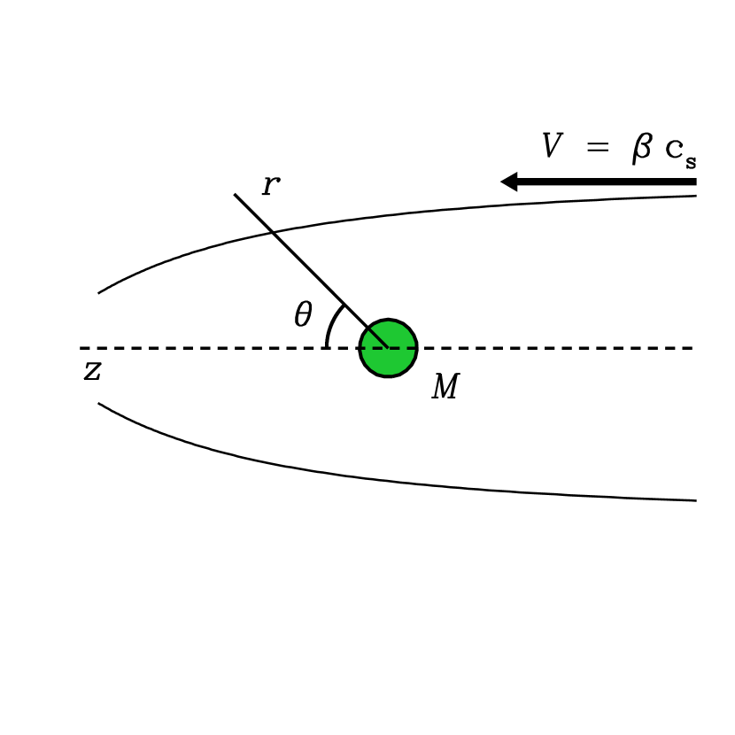
Let the gravitating mass $M$ travel in a straight line with speed $V$ through the extended gas cloud. Following previous analytic studies of dynamical friction, we assume the gas to be isothermal, with an associated sound speed $c_{s}$. Very far from the mass, the density is spatially uniform and has the value $\rho_{0}$. We choose a reference frame whose origin is anchored on the perturbing mass. In this frame, it is the gas that has speed $V$ far from the mass. We let the gas velocity be directed along the $z$-axis, and employ spherical coordinates $r$ and $\theta$ (see Fig. 1). We now seek a steady-state, axisymmetric solution for the flow, which is taken to be inviscid. We neglect the self-gravity of the gas, and assume that each fluid element feels only a pressure gradient and the gravitational pull of the point mass.

Figure 1: Spherical coordinate system centered on a gravitating body of mass $M$. The gas is isothermal, and its velocity far upstream is $\beta\,c_{\rm s}\ (\beta<1)$. The upstream direction corresponds to $\theta=\pi$, and downstream to $\theta=0$. While the figure shows the mass to have a finite physical size, we assume it to be a point particle in our analysis.

Strictly speaking, there is no steady flow, as this mass decelerates and $V$ continually changes (e.g., Fathi, 2010). What, then, is the meaning of the force we are calculating? Imagine the object being dragged by a massless string through the gas at the fixed speed $V$. After a long time, a steady-state flow is indeed established throughout the surrounding gas, and the tension in the string approaches a constant value. This limiting tension is the dynamical friction force being calculated here.

Return now to the actual case, in which there is no string and the mass decelerates. As stated previously, there is no global, steady-state flow. The flow is quasi-steady, however, within some distance over which the altered motion of the mass is communicated by sound waves. We shall quantify this distance later, after we have established the flow assuming steady-state conditions.

One important property of the flow is that it is irrotational. Euler’s equation in steady state may be written

$$\boldsymbol{u}\times\boldsymbol{\omega}\,=\,\boldsymbol{\nabla}B\,\,,$$ (1)

where $\boldsymbol{u}$ is the fluid velocity, $\boldsymbol{\omega}\,\equiv\boldsymbol{\nabla}\times\boldsymbol{u}$ is the vorticity, and the Bernoulli function $B$ is

$$B\,\equiv\,{1\over 2}\,u^{2}\,+\,c_{s}^{2}\,\,{\rm ln}\left(\,{\rho\over{\rho_{0}}}\right)\,-\,\frac{G\,M}{r}\,\,.$$ (2)

Both the fluid speed and density approach constant values far from the mass. Hence, $B$ is a spatial constant throughout the flow, and

$$\boldsymbol{u}\times\boldsymbol{\omega}\,=\,0\,\,.$$ (3)

Since $\boldsymbol{u}$ is a poloidal vector, the vorticity $\boldsymbol{\omega}$ is toroidal. The last equation then implies that $\boldsymbol{\omega}\,=\,0$, as claimed. We will not need to invoke the irrotational character of the flow until Section 5, when we explicitly evaluate the dynamical friction force.

Throughout our analysis, it will be more convenient to employ, not the vector fluid velocity $\boldsymbol{u}(r,\theta)$, but the scalar stream function $\psi(r,\theta)$. We may recover the individual velocity components from the stream function through the standard relations

$$u_{r}\, = \,{1\over{\rho\,r^{2}\,{\rm sin}\,\theta}}\,\,{{\partial\psi}\over{\partial\theta}}\,\,,$$ (4)

$$u_{\theta}\, = \,{-1\over{\rho\,r\,{\rm sin}\,\theta}}\,\,{{\partial\psi}\over{\partial r}}\,\,,$$ (5)

where $\rho\,=\,\rho(r,\theta)$ is the mass density. The velocity, as given by equations (4) and (5), automatically obeys mass continuity:

$$0\, = \,\boldsymbol{\nabla}\boldsymbol{\cdot}(\rho\,\boldsymbol{u})\,\,,$$

$$0\, = \,{1\over r^{2}}\,{\partial{\phantom{r}}\over{\partial r}}\left(\rho\,r^{2}\,u_{r}\right)\,+\,{1\over{r\,{\rm sin}\,\theta}}\,{\partial{\phantom{\theta}}\over{\partial\theta}}\left(\rho\,{\rm sin}\,\theta\,u_{\theta}\right)\,\,.$$ (6)

2.2 Perturbation Expansion

Far from the mass, as the density approaches $\rho_{0}$, the velocity has only a $z$-component, which is $V$. Equivalently, we have in this limit $u_{r}\,\approx\,V\,{\rm cos}\,\theta$ and $u_{\theta}\,\approx\,-V\,{\rm sin}\,\theta$. It follows that the far-field limit of the stream function is

$$\psi\,\approx\,{{\rho_{0}\,V\,r^{2}\,{\rm sin}^{2}\,\theta}\over 2}\,\,.$$ (7)

For a more complete analysis of the flow in this region, we take equation (7) to represent the leading term of a perturbation expansion. Introducing the sonic radius $r_{s}\,\equiv\,G\,M/c_{s}^{2}$, we first rewrite equation (7) as

$$\psi\,\approx\,\rho_{0}\,c_{s}\,r_{s}^{2}\,\beta\,\left({r\over r_{s}}\right)^{2}\,{{{\rm sin}^{2}\,\theta}\over 2}\,\,,$$ (8)

where $\beta$ is the Mach number of the projectile mass:

$$\beta\,\equiv\,{V\over c_{s}}\,\,.$$ (9)

Our perturbation expansion of $\psi$ is then given by

$$\psi\,=\,\rho_{0}\,c_{s}\,r_{s}^{2}\,\left[f_{2}\left(r\over r_{s}\right)^{2}\,+\,f_{1}\left(r\over r_{s}\right)\,+\,f_{0}\,+\,f_{-1}\left(r\over r_{s}\right)^{-1}\,+\,...\,\right]\,\,,$$ (10)

where

$$f_{2}\,\equiv\,{{\beta\,\,{\rm sin}^{2}\,\theta}\over 2}\,\,,$$ (11)

and where $f_{1}$, $f_{0}$, $f_{-1}$, etc. are still unknown, nondimensional functions of $\beta$ and $\theta$. Similarly, we expand the density as

$$\rho\,=\,\rho_{0}\,\left[1\,+\,g_{-1}\left({r\over r_{s}}\right)^{-1}\,+\,g_{-2}\left({r\over r_{s}}\right)^{-2}\,+\,g_{-3}\left({r\over r_{s}}\right)^{-3}\,+\,...\,\right]\,\,.$$ (12)

Here, $g_{-1}$, $g_{-2}$, $g_{-3}$, etc. are also nondimensional functions of $\beta$ and $\theta$, all yet to be found. Both expansions are only valid for $r\,\gg\,r_{s}$, the inequality that defines our outer region. We further assume that the physical radius of the object obeys $R\,\ll\,r_{s}$. Since the motion is subsonic ($V\,<\,c_{s}$), it follows that $R\,\ll\,r_{\rm acc}$, so that mass accretion is significant.

At this point, it is convenient to cast all our variables into nondimensional form. We let the fiducial radius, density, and speed be $r_{s}$, $\rho_{0}$, and $c_{\rm s}$, respectively. Similarly, the stream function is normalized to $\rho_{0}\,c_{s}\,r_{s}^{2}$. Then equations (4) and (5) relating the velocity to the stream function remain the same nondimensionally. We shall not employ a new notation for nondimensional variables, but make it clear whenever we switch back to dimensional relations. With this convention, the nondimensional expansions for the stream function and density simplify to

$$\psi\, = \,f_{2}\ r^{2}\,\,+\,\,f_{1}\ r\,\,+\,\,f_{0}\,\,+\,\,f_{-1}\ r^{-1}\,\,+\,...\,\,,$$ (13)

$$\rho\, = \,1\,\,+\,\,g_{-1}\ r^{-1}\,\,+\,\,g_{-2}\ r^{-2}\,\,+\,\,g_{-3}\ r^{-3}\,\,+\,\,...\,\,.$$ (14)

By adopting these perturbation expansions, we have effectively limited our analysis to the subsonic regime. For $\beta\,>\,1$, we expect the fluid variables or their derivatives to be discontinuous across the Mach cone, whose opening angle is given by ${\rm sin}\,\theta\,=\,\beta^{-1}$ (see, e.g., Ruderman & Spiegel, 1971). It would thus be necessary to adopt two separate expansions for $\psi$ and $\rho$, one inside and one outside the Mach cone. To avoid this complication, and since we are primarily interested in the subsonic regime in any event, we assume that $\beta\,<\,1$ and retain the single expansions.

2.3 Boundary Conditions

By symmetry, the upstream axis of the flow, defined by $\theta\,=\,\pi$, is a streamline for any $\beta$-value. That is, $\psi(r,\pi)$ is independent of $r$. The actual value of $\psi(r,\pi)$ is immaterial, reflecting the fact that the full function $\psi(r,\theta)$ can have an arbitrary additive constant without affecting the velocities. For convenience, we set $\psi(r,\pi)\,=\,0$, and note from equation (11) that $f_{2}(\pi)$ already vanishes. From equation (13) for the general expansion, we require that $f_{i}(\pi)\,=\,0$, for $i\,=\,1,\,0\,,-1,\,-2$, etc.

A second set of boundary conditions pertains to the behavior of the velocity $\boldsymbol{u}$. Let us focus again on the upstream axis. The righthand sides of both equations (4) and (5) contain ${\rm sin}\,\theta$ in the denominator. Since the density $\rho$ is finite at $\theta\,=\,\pi$, where ${\rm sin}\,\theta$ vanishes, both $\partial\psi/\partial\theta$ and $\partial\psi/\partial r$ must tend to zero as $\theta$ approaches $\pi$, at least as fast as ${\rm sin}\,\theta$.

Considering first $\partial\psi/\partial\theta$, we see that $\partial f_{2}/\partial\theta\,=\,\beta\,{\rm sin}\,\theta\,{\rm cos}\,\theta$, which properly vanishes. We must further demand that $f_{i}^{\prime}\,(\pi)\,=\,0$, for $i\,=\,1,\,0\,,-1,\,-2$, etc. Turning to $\partial\psi/\partial r$, the term involving $f_{2}$ still goes to zero, while $f_{0}(\theta)$ itself vanishes when taking the $r$-derivative of $\psi$. We are already requiring that $f_{i}\,(\pi)\,=\,0$ for all other $i$. Thus, the stipulation that $\psi\,(r,\pi)\,=\,0$ implies that $\partial\psi/\partial r$ also vanishes at $\theta\,=\,\pi$, so that $u_{\theta}$ does not diverge.

Approaching the downstream axis, ${\rm sin}\,\theta$ again vanishes as $\theta$ goes to zero. By analogous reasoning, we require that $f_{i}^{\prime}\,(0)\,=\,0$ for $i\,=\,1,\,0\,,-1,\,-2$, etc. To ensure the regularity of $u_{\theta}$, we further need $f_{i}\,(0)\,=\,0$, for $i\,=\,1,\,-1,\,-2$, etc. Again, the term $f_{0}$ disappears when taking the $r$-derivative of $\psi$, and there is no a priori restriction on $f_{0}\,(0)$. Indeed, this quantity sets the mass accretion rate onto the moving body, as we later demonstrate. In summary, our boundary conditions are: $f_{i}\,(\pi)\,=\,f_{i}^{\prime}\,(\pi)\,=\,f_{i}^{\prime}\,(0)\,=\,0$, for $i\,=\,1,\,0\,,-1,\,-2$, etc., and $f_{i}\,(0)\,=\,0$ for $i\,=\,1,\,-1,\,-2$, etc.

3 Outer Flow: Results

3.1 First-Order Equations

Our inviscid flow obeys Euler’s equation, which we write in spherical coordinates. The $r$- and $\theta$-components of this vector equation are

$$u_{r}\,{{\partial u_{r}}\over{\partial r}}\,+\,{u_{\theta}\over r}\,{{\partial u_{r}}\over{\partial\theta}}\,-\,{{u_{\theta}^{2}}\over r}\, = \,-{1\over\rho}\,{{\partial\rho}\over{\partial r}}\,-\,{1\over r^{2}}\,\,,$$ (15)

$$u_{r}\,{{\partial u_{\theta}}\over{\partial r}}\,+\,{u_{\theta}\over r}\,{{\partial u_{\theta}}\over{\partial\theta}}\,+\,{{u_{r}\,u_{\theta}}\over r}\, = \,-{1\over{\rho\,r}}\,{{\partial\rho}\over{\partial\theta}}\,\,,$$ (16)

where $u_{r}$ and $u_{\theta}$ are given in terms of $\psi$ by equations (4) and (5). Our strategy is to substitute the perturbation expansions (13) and (14) into Euler’s equations. For each power of $r$, we demand that its coefficients match. In this way, we will obtain a hierarchy of coupled equations for the functions $f$ and $g$.

Before proceeding, we first note that $u_{r}$ and $u_{\theta}$ are both proportional to $\rho^{-1}$. To avoid expanding inverse powers of the density, we multiply equations (15) and (16) through by $\rho^{3}$. Replacing the velocity components by derivatives of $\psi$ results in complex expressions that we shall not write out in full. We simply note, as an example, that the first lefthand term in the $r$-component of Euler’s equation is

$$\rho^{3}\,u_{r}\,{{\partial u_{r}}\over{\partial r}}\,=\,-{{2\,\rho}\over{r^{5}\,{\rm sin}^{2}\,\theta}}\left({{\partial\psi}\over{\partial\theta}}\right)^{2}\,-\,{1\over{r^{4}\,{\rm sin}^{2}\,\theta}}\,{{\partial\rho}\over{\partial r}}\left({{\partial\psi}\over{\partial\theta}}\right)^{2}\,+\,{1\over{r^{4}\,{\rm sin}^{2}\,\theta}}\,{{\partial\psi}\over{\partial\theta}}\,{{\partial^{2}\psi}\over{\partial r\partial\theta}}\,\,.$$ (17)

After substituting the series expansions for $\psi$ and $\rho$, we find that the highest power of $r$ is $r^{-1}$. In this case, all the coefficients on both sides of Euler’s equations vanish identically.

Matching the coefficients of $r^{-2}$, we obtain the first-order equations. From the $r$-component of Euler’s equation, we find

$$-\beta\,f_{1}^{\prime\prime}\,-\,\beta\,f_{1}\,+\,\beta^{2}\,{\rm sin}\,\theta\,{\rm cos}\,\theta\,\,g_{-1}^{\prime}\,+\,\left(\beta^{2}\,{\rm cos}^{2}\,\theta\,\,-\,1\right)\,g_{-1}\,+\,1\,=\,0\,\,,$$ (18)

while the $\theta$-component yields

$$\left(1\,-\,\beta^{2}\,{\rm sin}^{2}\,\theta\right)\,g_{-1}^{\prime}\,-\,\beta^{2}\,{\rm sin}\,\theta\,{\rm cos}\,\theta\,\,g_{-1}\,=\,0\,\,.$$ (19)

In both of these equations and those that follow, a prime denotes a $\theta$-derivative.

These equations govern the first non-trivial terms in the expansions for $\psi$ and $\rho$. Their solution, therefore, must be equivalent to that obtained through the more traditional, linear analysis. Integrating equation (19), we find

$$g_{-1}\,=\,{C\over{\left(1\,-\,\beta^{2}\,{\rm sin}^{2}\,\theta\right)^{1/2}}}\,\,,$$ (20)

where $C$ is a constant, as yet undetermined. In the subsonic regime, the denominator on the righthand side does not vanish for any $\theta$, and $g_{-1}$ remains finite.

Substituting this expression for $g_{-1}$ into (18) gives the equation obeyed by $f_{1}$:

$$f_{1}^{\prime\prime}\,+\,f_{1}\,=\,{1\over\beta}\,-\,{{C\,\left(1\,-\,\beta^{2}\right)}\over{\beta\left(1\,-\,\beta^{2}\,{\rm sin}^{2}\,\theta\right)^{3/2}}}\,\,.$$ (21)

A particular solution of this equation may be found through the method of variation of parameters. Adding the two homogeneous solutions yields

$$f_{1}\,=\,{1\over\beta}\,-\,{{C\,\left(1\,-\,\beta^{2}\,{\rm sin}^{2}\,\theta\right)^{1/2}}\over\beta}\,+\,D\,{\rm cos}\,\theta\,+\,E\,{\rm sin}\,\theta\,\,,$$ (22)

where $D$ and $E$ are also constants.

We proceed to evaluate the constants through application of the boundary conditions. The requirement that $f_{1}(\pi)\,=\,0$ gives

$$C\,=\,1\,-\,\beta\,D\,\,.$$ (23)

Similarly, we have $f_{1}(0)\,=\,0$, yielding

$$C\,=\,1\,+\,\beta\,D\,\,.$$ (24)

It follows, from these last two relations, that $C\,=\,1$ and $D\,=\,0$. Finally, we have $f_{1}^{\prime}(\pi)\,=\,0$, from which we infer that $E\,=\,0$. It may be verified that the boundary condition $f_{1}^{\prime}(0)\,=\,0$ is then also satisfied.

In summary, the first-order density and stream function perturbations are

$$g_{-1}\, = \,{1\over{\left(1\,-\,\beta^{2}\,{\rm sin}^{2}\,\theta\right)^{1/2}}}\,\,,$$ (25)

$$f_{1}\, = \,{{1\,-\,\left(1\,-\,\beta^{2}\,{\rm sin}^{2}\,\theta\right)^{1/2}}\over\beta}\,\,.$$ (26)

Notice that $g_{-1}^{\prime}\,=\,0$ at both $\theta\,=\,0$ and $\pi$, implying that the density profile is flat (i.e., does not have a cusp) on either the upstream or downstream axis. Our expression for $g_{-1}$ is consistent with the linear density perturbation obtained by Dokuchaev (1964), Ruderman & Spiegel (1971), and Ostriker (1999). Notice that $g_{-1}(\pi/2)$ diverges as $\beta$ approaches unity, signifying the birth of the Mach cone. Our $f_{1}$, in combination with $g_{-1}$, yields the linear velocity components given in equations (25) and (26) of Dokuchaev (1964).

Figure 2 displays the streamlines (solid curves) and isodensity contours (dashed curves) for the outer flow, including only the first-order perturbations. The light, dotted circle marks the sonic radius, $r\,=\,1$; the solution is only accurate well outside this sphere. Notice how all curves and contours are symmetric about the $\theta\,=\,\pi/2$ plane. The streamlines, in particular, show the fluid veering toward the mass, but then turning away again. We cannot detect true accretion of mass or linear momentum until we include the next higher-order perturbations.

Figure 2: Streamlines (solid) and density contours (dashed) for the $\beta=0.5$ flow, including only first-order perturbations. All quantities shown are nondimensional. The density contours correspond to $\rho=1.2,1.4,$ and 1.6, while adjacent streamlines enclose equal mass fluxes. The inner dotted circle has the sonic radius. Since the streamlines and density contours are symmetric upstream and downstream, we cannot determine the true accretion rates of mass and momentum without higher-order perturbations.

3.2 Second-Order Equations

We next equate coefficients of $r^{-3}$ in both components of Euler’s equation. From the $r$-component, equation (15), we obtain one relation between $f_{0}$ and $g_{-2}$:

$$-\beta\,f_{0}^{\prime\prime}\,-\,\beta\,{\rm cot}\,\theta\,f_{0}^{\prime}\,+\,\ \beta^{2}\,{\rm sin}\,\theta\,{\rm cos}\,\theta\,\,g_{-2}^{\prime}\,+\,\left(2\,\beta^{2}\,{\rm cos}^{2}\,\theta\,-\,2\right)\,g_{-2}\,=\,{\cal A}_{1}\,+\,{\cal A}_{2}\,+\,{\cal A}_{3}\,\,.$$ (27)

Here, ${\cal A}_{1}$, ${\cal A}_{2}$, and ${\cal A}_{3}$ are expressions involving $f_{1}$ and $g_{-1}$:

$${\cal A}_{1}\, \equiv \,{f_{1}^{2}\over{{\rm sin}^{2}\,\theta}}\,-\,{{f_{1}\,f_{1}^{\prime}\,{\rm cos}\,\theta}\over{{\rm sin}^{3}\,\theta}}\,+\,{{\left(f_{1}^{\prime}\right)^{2}}\over{{\rm sin}^{2}\,\theta}}\,+\,{{f_{1}\,f_{1}^{\prime\prime}}\over{{\rm sin}^{2}\,\theta}}\,\,,$$ (28)

$${\cal A}_{2}\, \equiv \,\beta\,f_{1}\,\,g_{-1}\,-\,2\,\beta\,f_{1}^{\prime}\,\,g_{-1}\,{\rm cot}\,\theta\,-\,\beta\,f_{1}\,\,g_{-1}^{\prime}\,{\rm cot}\,\theta\,-\,\beta\,f_{1}^{\prime}\,\,g_{-1}^{\prime}\,+\,\beta\,f_{1}^{\prime\prime}\,\,g_{-1}\,\,,$$ (29)

$${\cal A}_{3}\, \equiv \,2\,g_{-1}^{2}\,-\,3\,g_{-1}\,\,.$$ (30)

From the $\theta$-component, equation (16), we obtain a second relation between $f_{0}$ and $g_{-2}$:

$$-\beta\,f_{0}^{\prime}\,+\,{\cal D}\,g_{-2}^{\prime}\,-\,2\,\beta^{2}\,{\rm sin}\,\theta\,\,{\rm cos}\,\theta\,\,g_{-2}\,=\,{\cal B}_{1}\,+\,{\cal B}_{2}\,+\,{\cal B}_{3}\,\,,$$ (31)

where we have defined ${\cal D}\,\equiv\,1\,-\,\beta^{2}\,{\rm sin}^{2}\,\theta$, and where the three terms on the righthand side are again combinations of $f_{1}$ and $g_{-1}$:

$${\cal B}_{1}\, \equiv \,f_{1}^{2}\,\frac{{\rm cot}\,\theta}{\sin^{2}\theta}\,-\,{{f_{1}\,f_{1}^{\prime}}\over{{\rm sin}^{2}\,\theta}}\,\,,$$ (32)

$${\cal B}_{2}\, \equiv \,\beta\,f_{1}\,\,g_{-1}\,{\rm cot}\,\theta\,\,+\,\,\beta\,f_{1}^{\prime}\,\,g_{-1}\,\,+\,\,2\,\beta\,f_{1}\,g_{-1}^{\prime}\,\,,$$ (33)

$${\cal B}_{3}\, \equiv \,-2\,g_{-1}\,\,g_{-1}^{\prime}\,\,.$$ (34)

We have already found $f_{1}$ and $g_{-1}$ in the subsonic case of interest. After substituting these expressions, equations (25) and (26), into the righthand sides of equations (27) and (31), the coupled equations for $f_{0}$ and $g_{-2}$ become:

$$-\beta\,f_{0}^{\prime\prime}\,-\,\beta\,{\rm cot}\,\theta\,f_{0}^{\prime}\,+\,\ \beta^{2}\,{\rm sin}\,\theta\,{\rm cos}\,\theta\,\,g_{-2}^{\prime}\,+\,\left(2\,\beta^{2}\,{\rm cos}^{2}\,\theta\,-\,2\right)\,g_{-2}\,=\,{1\over{\cal D}}\,-\,{3\over\sqrt{\cal D}}\,+\,{2\over{1+\sqrt{\cal D}}}\,\,,$$ (35)

and

$$-\beta\,f_{0}^{\prime}\,+\,{\cal D}\,g_{-2}^{\prime}\,-\,2\,\beta^{2}\,{\rm sin}\,\theta\,\,{\rm cos}\,\theta\,\,g_{-2}\,=\,\beta^{2}\,{\rm sin}\,\theta\,\,{\rm cos}\,\theta\left[-{2\over{{\cal D}^{2}}}\,+\,{2\over{{\cal D}^{3/2}}}\,-\,{1\over{\cal D}}\,+\,{1\over{\left(1+\sqrt{\cal D}\right)^{2}}}\right]\,\,.$$ (36)

These last two relations constitute our second-order equations. For any value of $\beta$, we may integrate them numerically from the upstream axis, $\theta\,=\,\pi$, to the downstream axis at $\theta\,=\,0$. Three initial conditions are required, of which we have already identified two: $f_{0}(\pi)\,=\,f_{0}^{\prime}(\pi)\,=\,0$. As a third initial condition, we use $g_{-2}(\pi)$, whose value at this point is arbitrary. For each chosen value of $g_{-2}(\pi)$, we may find $f_{0}(\theta)$ and $g_{-2}(\theta)$. We thus have a one-parameter family of outer flow solutions.

In the upper panel of Figure 3 we display, for the representative value $\beta\,=\,0.5$, three solutions of $g_{-2}(\theta)$. We obtained each solution by assuming different values of $g_{-2}(\pi)$. Notice that $g_{-2}^{\prime}$ vanishes on the upstream and downstream axes, implying again that the density profile is flat in both regions. Notice also that all curves attain the same value at $\theta\,=\,\pi/2$. That is, $g_{-2}(\pi/2)$ depends only on $\beta$, and not on the prescribed initial condition $g_{-2}(\pi)$.

The lower panel of Figure 3 shows the corresponding plots of $f_{0}(\theta)$. We see that $f_{0}^{\prime}(0)\,=\,0$ in every case, ensuring regularity of $u_{r}$ on the downstream axis. This condition was not imposed a priori, but resulted automatically from integration of the governing equations. Specifically, the coefficient of $f_{0}^{\prime}$ in equation (35) includes ${\rm cot}\,\theta$, which diverges at $\theta\,=\,0$. Since all the other terms in this equation remain finite on the axis, $f_{0}^{\prime}(0)$ is forced to zero.

Figure 3: Sample solutions to the second-order perturbation equations (35) and (36), for $g_{-2}(\theta)$ (upper panel) and $f_{0}(\theta)$ (lower panel). The initial values of $g_{-2}(\pi)$ are +1.12 (dotted), +0.12 (solid), and -0.88 (dashed).

Which of these solutions is the true outer flow for gas that is accreting steadily onto the gravitating mass? In principle, one could answer this question by continuing each solution inward, to see if the flow smoothly crosses the sonic surface, where $u\,=\,1$. We shall not attempt such a calculation here. Instead, we will proceed by determining generically the mass accretion rate that is associated with each outer solution. Then, given the Bondi prescription for this rate, we will indeed be able to select the physical solution for each $\beta$.

4 Mass Accretion Rate

4.1 Relation to Stream Function

One could, in principle, equate coefficients of $r^{-4}$, $r^{-5}$, etc., and thereby obtain the coupled equations linking higher-order $f$- and $g$-variables. We will now demonstrate, however, that the first- and second-order equations just presented are sufficient to establish the total accretion rate onto the mass. We will then relate, in Section 5 below, this infall rate to the desired friction force.

Refer again to Figure 1 and imagine a sphere of radius $r$ surrounding the mass. Reverting temporarily to dimensional variables, the mass accretion rate is

$${\dot{M}}\, = \,-2\,\pi\int_{0}^{\pi}\!\rho\,u_{r}\,r^{2}\,{\rm sin}\,\theta\,d\theta$$ (37)

$$= \,-2\,\pi\int_{0}^{\pi}\!{{\partial\psi}\over{\partial\theta}}\,d\theta$$ (38)

$$= \,2\,\pi\,\left[\psi(r,0)\,-\,\psi(r,\pi)\right]\,\,,$$ (39)

where we have utilized equation (4) connecting $u_{r}$ and $\psi$. Recall that $\psi(r,\pi)$ is actually a constant, independent of $r$, and that we have set that constant to zero. We thus have

$${\dot{M}}\,=\,2\,\pi\,\psi(r,0)\,\,.$$ (40)

To nondimensionalize this result, we first set the fiducial mass accretion rate to $2\,\pi\,\rho_{0}\,c_{s}\,r_{s}^{2}$. After using the expansion of $\psi$ from equation (13), we obtain the nondimensional equation

$${\dot{M}}\,=\,f_{2}(0)\,r^{2}\,+\,f_{1}(0)\,r\,+\,f_{0}(0)\,+\,f_{-1}(0)\,r^{-1}\,+\,f_{-2}(0)\,r^{-2}\,\,...\,\,.$$ (41)

One of our boundary conditions, ensuring regularity of $u_{\theta}$ on the downstream axis, is that $f_{i}(0)\,=\,0$ for $i\,=\,1,\,-1,\,-2,\,$ etc. Since $f_{2}(0)\,=\,0$, we find the simple relation

$${\dot{M}}\,=\,f_{0}(0)\,\,.$$ (42)

Both sides in this equation are functions of $\beta$, although we have not indicated the dependence explicitly. In any case, the relation confirms our expectation that the mass accretion rate is independent of the sphere’s radius $r$ in steady-state motion. We also now see that the higher-order variables $f_{-1}$, $f_{-2}$, etc. play no part in determining this rate.

4.2 Relation to Density Perturbation

Now that we have tied the mass accretion rate to $f_{0}(0)$, we can immediately rule out a subset of outer flow solutions as being unphysical. Figure 3 shows that, for $g_{-2}(\pi)\,=\,1.12$, $f_{0}(0)$ is negative, corresponding to a net mass efflux. That such a situation is even possible emphasizes once more the need to extend the flow solution inward across the sonic surface.

For this same choice of $g_{-2}(\pi)$, the dotted curve in the lower panel of Figure 3 shows that $g_{-2}(0)\,<\,g_{-2}(\pi)$. Indeed, we have just found one example of a general result: the difference $g_{-2}(0)\,-\,g_{-2}(\pi)$ agrees in sign with $f_{0}(0)$. We now show that the two quantities are in fact equal, apart from a multiplicative factor.

Our proof starts with the fact that the lefthand side of the second-order equation (36) is a perfect derivative. Specifically,

$$-\beta\,f_{0}^{\prime}\,+\,{\cal D}\,g_{-2}^{\prime}\,-\,2\,\beta^{2}\,{\rm sin}\,\theta\,\,{\rm cos}\,\theta\,\,g_{-2}\,\,=\,\,{{d{\phantom{\theta}}}\over{d\,\theta}}\left(-\beta\,f_{0}\,+\,{\cal D}\,g_{-2}\right)\,\,.$$ (43)

Turning to the righthand side of the same equation, we note first that ${\rm sin}\,\theta$ is an even function of $\theta-\pi/2$, while ${\rm cos}\,\theta$ is an odd function. Since $\cal D$ depends only on ${\rm sin}\,\theta$, it has even symmetry. Inspection shows that the righthand side of equation (36) has odd symmetry.

If we now integrate equation (36) from $\theta\,=\,\pi$ to 0, the righthand side vanishes because of the odd symmetry of the integrand. We find that

$$\left(-\beta\,f_{0}\,+\,{\cal D}\,g_{-2}\right)_{\theta\,=\,\pi}\,=\,\left(-\beta\,f_{0}\,+\,{\cal D}\,g_{-2}\right)_{\theta\,=\,0}\,\,.$$ (44)

Since $f_{0}(\pi)\,=\,0$ and ${\cal D}(\pi)\,=\,{\cal D}(0)\,=\,1$, we have

$$g_{-2}(\pi)\,=\,-\beta\,f_{0}(0)\,+\,g_{-2}(0)\,\,,$$ (45)

which we recast as

$$f_{0}(0)\,=\,{{g_{-2}(0)\,-\,g_{-2}(\pi)}\over\beta}\,\,.$$ (46)

Recalling equation (42) that identifies $f_{0}(0)$ as the mass accretion rate, we now see that this rate is proportional to the difference, upstream and downstream, of the second-order density perturbation. As $\beta$ approaches zero, these two perturbations become equal. Indeed, the function $g_{-2}(\theta)$ is a constant (equal to 1/2) in the limit, consistent with a spherically symmetric flow.

4.3 Modified Bondi Prescription

To establish the physically relevant flow solutions, we need to specify the accretion rate as a function of velocity. Bondi (1952) fully solved the $\beta\,=\,0$ problem. That is, he determined the complete distribution of density and velocity surrounding a mass at rest within a background gas. Dimensionally, he found for the mass accretion rate

$${\dot{M}}\,=\,{{4\,\pi\,\lambda\,\rho_{0}\,G^{2}\,M^{2}}\over{c_{s}^{3}}}\,\,,$$ (47)

where $\lambda\,=\,{\rm e}^{3/2}/4\,=\,1.12$ for the isothermal case of interest here. Recasting the rate into nondimensional form (recall Section 4.1), we have

$$\lim_{\beta\,\rightarrow\,0}\,\,{\dot{M}}\, = \,2\,\lambda$$

$$= \,{{{\rm e}^{3/2}}\over 2}\,\,,$$ (48)

as one constraint on the general form of $\dot{M}(\beta)$.

Prior to Bondi’s work, Hoyle & Lyttleton (1939) studied accretion onto a mass traveling through a zero-temperature gas. Their dimensional result was

$${\dot{M}}\,=\,{{4\,\pi\,\rho_{0}\,G^{2}\,M^{2}}\over{V^{3}}}\,\,.$$ (49)

Noting that the Mach number $\beta$ is effectively infinite in this case, the equivalent, nondimensional finding is

$$\lim_{\beta\,\rightarrow\,\infty}\,\,{\dot{M}}\,=\,{2\over{\beta^{3}}}\,\,.$$ (50)

Bondi & Hoyle (1944) later showed that this relation provides an upper bound to the accretion rate in the zero-temperature case. Through more careful analysis of the wake, which here degenerates into an infinite-density spindle, they set the lower limit a factor of two smaller.

The widely used interpolation formula of Bondi (1952) connects these limits, at least approximately. Nondimensionally, the Bondi prescription is

$${\dot{M}}(\beta)\,=\,{1\over{\left(1\,+\,\beta^{2}\right)^{3/2}}}\,\,.$$ (51)

In the low-$\beta$ limit, $\dot{M}$ falls short of the isothermal result, but matches that for a $\gamma\,=\,3/2$ polytrope. The high-$\beta$ limit reproduces the lower bound established by Bondi & Hoyle (1944).

Since we are focusing on the subsonic regime within an isothermal gas, we want our low-$\beta$ limit to agree with the exact result. Following Moeckel & Throop (2009), we adopt a modified form of the classic interpolation formula:

$${\dot{M}}(\beta)\,=\,{{2\,\left(\lambda^{2}\,+\,\beta^{2}\right)^{1/2}}\over{\left(1\,+\,\beta^{2}\right)^{2}}}\,\,,$$ (52)

where we use the isothermal value of $\lambda$ previously given. For $\beta\,\ll\,1$, $\dot{M}$ approaches the result of Bondi (1952) given in equation (48). For $\beta\,\gg\,1$, we recover the upper limit of Bondi & Hoyle (1944). In the simulation of Moeckel & Throop (2009) for an isothermal gas with $\beta=10$, this modified interpolation formula matches the calculated accretion rate to within 20 percent. Judging from their own polytropic simulations, both Hunt (1971) and Shima, Matsuda, Takeda, & Sawada (1985) had earlier suggested that the original Bondi $\dot{M}(\beta)$ be augmented by about a factor of two. In summary, equation (52) should be sufficiently accurate for our purposes.

The combination of equations (42) and (52) gives us the proper value of $f_{0}(0)$ at each $\beta$, and thus also establishes the physically relevant outer flow solutions. Figure 4 shows the physical $f_{0}(0)$ and $g_{-2}(\pi)$ as functions of $\beta$. Note that the latter diverges as $\beta$ approaches unity. Thus, our perturbation series fails to describe the flow along the upstream axis in this limit. As we will show in the next section, however, the dynamical friction force remains finite for all $\beta$.

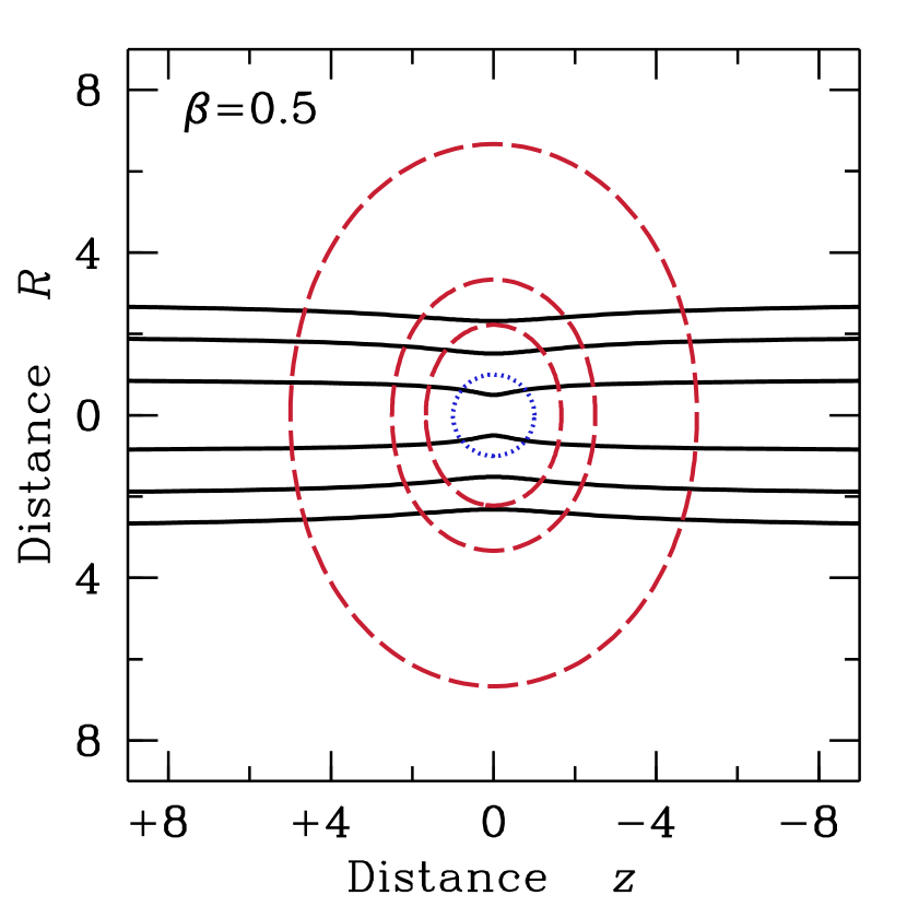
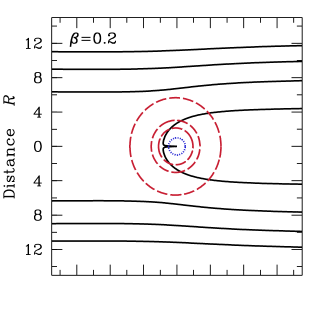
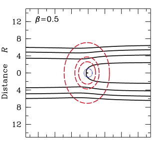
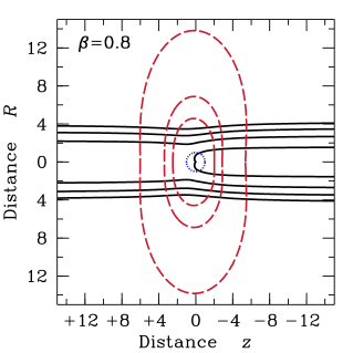
The three panels of Figure 5 display streamlines and isodensity contours for the indicated $\beta$-values. These curves were constructed from equations (13) and (14) for $\psi$ and $\rho$, respectively, using the three known terms in each series. The circle in each panel represents the sonic surface. As always, our results are only accurate well beyond this radius.

Figure 4: The upstream density perturbation $g_{-2}(\pi)$ for the physical accretion flow, shown as a function of Mach number $\beta$. This initial condition gives the correct $\dot{M}=f_{0}(0)$, also shown in the figure.

Figure 5: Streamlines (solid) and density contours (dashed) for three different Mach numbers $\beta$. The density contours correspond to $\rho=1.2,1.4,$ and 1.6. The innermost streamlines enclose the full mass accretion rate $\dot{M}$. Successive streamlines enclose 3, 5, and 7 times this rate. As in Figure 2, the inner circle represents the sonic surface.

5 Friction Force

5.1 Integral Expression

The dynamical friction force $F$ is the total rate at which $z$-momentum is transferred from the background gas to the gravitating mass. Within our steady-state flow, the total momentum transfer rate into a surface surrounding the mass is independent of the size and shape of that surface, provided it lies outside the wake, where the physical interaction between the projectile and gas occurs. The net momentum flow calculated through such a surface integration all goes into the gravitating mass, causing its deceleration.

Imagine the gravitating mass to be surrounded by a large sphere of radius $r$. In part, the $z$-momentum transfer arises from the advection of this quantity in the flowing gas across the spherical surface. Since the inward flux of $z$-momentum is $-\rho\,u_{r}\,u_{z}$ the kinetic portion of $F$ is, dimensionally,

$$F_{\rm kin}\,=\,-2\,\pi\,\int_{0}^{\pi}\!\rho\,u_{r}\,u_{z}\,r^{2}\,{\rm sin}\,\theta\,d\theta\,\,.$$ (53)

Another contribution to $F$ is from the thermal pressure of the surrounding gas. This static portion of the force is

$$F_{\rm static}\,=\,-2\,\pi\,\int_{0}^{\pi}\!\rho\,c_{s}^{2}\,r^{2}\,{\rm cos}\,\theta\,{\rm sin}\,\theta\,d\theta\,\,.$$ (54)

Adding these two pieces, we have, after nondimensionalization,

$$F\,=\,-\int_{0}^{\pi}\!\rho\,u_{r}\,u_{z}\,r^{2}\,{\rm sin}\,\theta\,d\theta\,-\,\int_{0}^{\pi}\!\rho\,r^{2}\,{\rm cos}\,\theta\,{\rm sin}\,\theta\,d\theta\,\,,$$ (55)

where we have set the unit of force equal to $2\,\pi\,\rho_{0}\,c_{s}^{2}\,r_{s}^{2}$.

The integrand within the first, righthand term must be recast in terms of the stream function:

$$\rho\,u_{r}\,u_{z}\,r^{2}\,{\rm sin}\,\theta\,=\,{{{\rm cot}\,\theta}\over{\rho\,r^{2}}}\left({{\partial\psi}\over{\partial\theta}}\right)^{2}\,+\,{1\over{\rho\,r}}{{\partial\psi}\over{\partial\theta}}{{\partial\psi}\over{\partial r}}\,\,.$$ (56)

We may now evaluate $F$ using the series expansions for $\psi$ and $\rho$. The full expression is a series of terms proportional to $r^{2}$, $r^{1}$, $r^{0}$, etc.

All terms in $F$ containing positive powers of $r$ vanish upon integration. Those proportional to $r^{1}$ involve $f_{1}$ and $g_{-1}$, both of which are known explicitly. Terms associated with negative powers of $r$ contain $f$- and $g$-variables which we have not yet calculated (e.g., $f_{-1}$, $g_{-3}$). However, as we consider ever larger radii $r$, where the series expansions themselves become increasingly accurate, these terms also go to zero. Only those independent of $r$ survive.

After restricting ourselves to $r$-independent terms, we find

$$F\,=\,-\int_{0}^{\pi}\!\left[\left(1-\beta^{2}\right)\,{\rm sin}\,\theta\,{\rm cos}\,\theta\,\,g_{-2}\,+\,\beta\left(1\,+\,{\rm cos}^{2}\,\theta\right)f_{0}^{\prime}\right]\!d\theta\,\,.$$ (57)

Here, we have omitted a number of terms in the integrand containing $f_{1}$, $g_{-1}$, and their derivatives. All of these terms are antisymmetric with respect to $\theta\,-\pi/2$ (i.e., they are odd functions), and therefore vanish upon integration.

5.2 Relation to Mass Accretion Rate

By dimensional considerations, the friction force should be $F\,=\,C{\dot{M}}\,V$, where $C$ is dimensionless. In the hypersonic limit, this multiplicative factor contains a Coulomb logarithm (e.g. Ruderman & Spiegel, 1971). We now demonstrate the surprising fact that, in the subsonic case of interest here, the factor is exactly unity. In fully nondimensional language, we shall prove that

$$F\,=\,{\dot{M}}\,\beta\,\,.$$ (58)

We begin by splitting the integral on the righthand side of equation (57) into two parts:

$$F\, = \,-\int_{0}^{\pi}\!\beta\,f_{0}^{\prime}\,d\theta\,-\,\int_{0}^{\pi}\!\left[\left(1-\beta^{2}\right)\,{\rm sin}\,\theta\,{\rm cos}\,\theta\,\,g_{-2}\,+\,\beta\,{\rm cos}^{2}\,\theta\,f_{0}^{\prime}\right]\!d\theta$$ (59a)

$$= \,\beta\,f_{0}(0)\,-\,{\cal I}\,\,$$ (59b)

$$= \,\beta\,\dot{M}\,-\,{\cal I}\,\,.$$ (59c)

In these equations, we have used the fact that $f_{0}(\pi)\,=\,0$ and $f_{0}(0)=\dot{M}$ (eq. 42). We have further defined

$${\cal I}\,\equiv\,\int_{0}^{\pi}\!d\theta\,\left[\left(1-\beta^{2}\right)\,{\rm sin}\,\theta\,{\rm cos}\,\theta\,\,g_{-2}\,+\,\beta\,{\rm cos}^{2}\,\theta\,f_{0}^{\prime}\right]\,\,.$$ (60)

We next show that $\cal I$ vanishes.

First recall that our flow is irrotational. Specifically, the $\phi$-component of the vorticity vanishes, so that

$$\frac{\partial\,u_{r}}{\partial\,\theta}\,-\,\frac{\left(r\,u_{\theta}\right)}{\partial\,r}\,=\,0\,\,.$$ (61)

Expressing both velocity components in terms of the stream function through equations (4) and (5), we have

$$\frac{\partial\rho}{\partial\theta}\,\frac{\partial\psi}{\partial\theta}\,+\,\rho\,{\rm cot}\,\theta\,\frac{\partial\psi}{\partial\theta}\,-\,\rho\,\frac{\partial^{2}\psi}{\partial\theta^{2}}\,+\,r^{2}\,\frac{\partial\rho}{\partial r}\,\frac{\partial\psi}{\partial r}\,-\,\rho\,r^{2}\,\frac{\partial^{2}\psi}{\partial r^{2}}\,=\,0\,\,.$$ (62)

We substitute the series expansions for $\psi$ and $\rho$ into this last equation and set the coefficients of all powers of $r$ to zero. Following this procedure for $r^{2}$ and $r^{1}$, and using the known expressions for $f_{2}$, $f_{1}$, and $g_{-1}$, yields identities. However, setting the $r$-independent terms to zero leads to a nontrivial result:

$$\beta\,f_{0}^{\prime\prime}\,-\,\beta\,{\rm cot}\theta\,f_{0}^{\prime}\,-\,\beta^{2}\,{\rm sin}\,\theta\,{\rm cos}\,\theta\,g_{-2}^{\prime}\,+\,2\,\beta^{2}\,{\rm sin}^{2}\,\theta\,g_{-2}\,=\,\frac{1\,-\,\sqrt{\cal D}}{\cal D}\,\,.$$ (63)

We add this last equation to the second-order equation (35), obtaining

$$2\,\left(\beta^{2}\,-\,1\right)g_{-2}\,-\,2\,\beta\,{\rm cot}\,\theta\,f_{0}^{\prime}\,=\,\frac{2}{\cal D}\,-\,\frac{4}{\sqrt{\cal D}}\,+\,\frac{2}{1\,+\,\sqrt{\cal D}}\,\,.$$ (64)

Multiplying through by $-(1/2)\,{\rm sin}\,\theta\,{\rm cos}\,\theta$ gives

$$\left(1\,-\,\beta^{2}\right){\rm sin}\,\theta\,{\rm cos}\,\theta\,g_{-2}\,+\,\beta\,{\rm cos}^{2}\,\theta\,f_{0}^{\prime}\,=\,-{\rm sin}\,\theta\,{\rm cos}\,\theta\left(\frac{1}{\cal D}\,-\,\frac{2}{\sqrt{\cal D}}\,+\,\frac{1}{1\,+\,\sqrt{\cal D}}\right)\,\,.$$ (65)

Integrating over $\theta$, we recognize the lefthand side of the resulting equation as $\cal I$. The righthand side vanishes, since the integrand is an odd function. We see therefore that equation (58) holds.

If we now employ the modified Bondi prescription, equation (52) for $\dot{M}$, we have an explicit expression for the force:

$$F\,=\,{{2\,\beta\,\left(\lambda^{2}\,+\,\beta^{2}\right)^{1/2}}\over{\left(1\,+\,\beta^{2}\right)^{2}}}\,\,.$$ (66)

Figure 6 displays the function $F(\beta)$. Also shown, as the dashed curve, is the result from Ostriker (1999) in which the force diverges as $\beta$ approaches unity. In the limit of low $\beta$, both forces rise linearly from zero at $\beta=0$, but our initial slope is larger by a factor of $3\lambda=3.36$. Indeed, over most $\beta$-values, our force exceeds that derived by Ostriker (1999), presumably because we have included both the gravitational tug from the wake and the direct accretion of momentum from the flow. Our force does not rise monotonically but instead peaks around $\beta=0.68$ and then begins to decline; we expect this decline to continue into the supersonic regime. We should bear in mind that, while equation (58) is exact, equation (66) for $F$ is only as accurate as the underlying interpolation formula.

Figure 6: The dimensionless friction force $F$ as a function of Mach number $\beta$. The dashed curve shows the force derived by Ostriker (1999), which diverges as $\beta$ approaches unity.

6 Velocity and Mass Evolution

Our simple result for the dynamical friction force means that the deceleration of the gravitating mass is also simply described, as long as there are no other forces at play. As we have stressed, the force is the rate at which gas transfers linear momentum to the object. But the object’s momentum is $MV$, where we now revert to dimensional variables. In the reference frame where the background gas is stationary, we have

$$\frac{d(MV)}{dt}\,=\,-{\dot{M}}\,V\,\,,$$ (67)

which implies that

$$\frac{1}{V}\,\frac{dV}{dt}\,=\,-\frac{2}{M}\,\frac{dM}{dt}\,\,.$$ (68)

If $V_{0}$ and $M_{0}$ are the object’s initial speed and mass, respectively, then

$$\frac{V}{V_{0}}\,=\,\left(\frac{M}{M_{0}}\right)^{-2}\,\,.$$ (69)

To track the speed as a function of time, we rewrite equation (52) for the mass accretion rate as

$$\frac{dM}{dt}\,=\,{{4\,\pi\,\rho_{0}\,c_{s}\,r_{s}^{2}\,\left(\lambda^{2}\,+\,\beta^{2}\right)^{1/2}}\over{\left(1\,+\,\beta^{2}\right)^{2}}}\left({M\over M_{0}}\right)^{2}\,\,.$$ (70)

Here, $\beta\,\equiv\,V/c_{\rm s}$ as before, while $r_{s}$ is now defined in terms of the initial mass: $r_{s}\equiv\,2\,G\,M_{0}/c_{s}^{2}$. The fully nondimensional evolutionary equation for the speed is then

$$\left(\frac{1}{\beta}\right)\,\frac{d\beta}{d\tau}\,=\,-{{4\,\left(\lambda^{2}\,+\,\beta^{2}\right)^{1/2}}\over{\left(1\,+\,\beta^{2}\right)^{2}}}\left(\frac{\beta}{\beta_{0}}\right)^{-1/2}\,\,.$$ (71)

In this last equation, we have introduced the initial, nondimensional speed $\beta_{0}$, as well as a nondimensional time, $\tau\,\equiv\,t/t_{0}$, where

$$t_{0}\, \equiv \,\frac{c_{s}^{3}}{2\,\pi\,\rho_{0}\,G^{2}\,M_{0}}$$ (72)

$$= \,\frac{M_{0}}{2\,\pi\,\rho_{0}\,c_{s}\,r_{s}^{2}}\,\,.$$ (73)

The denominator in equation (73) is the fiducial mass accretion rate defined in Section 4.1. Thus, $t_{0}$ is of order the accretion time onto the initial mass.

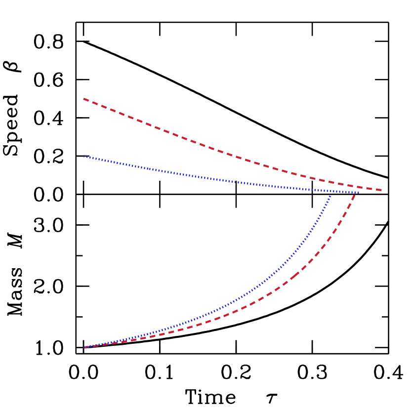
The upper panel of Figure 7 plots $\beta(\tau)$ for $\beta_{0}\,=\,0.2,\,0.5$ and 0.8, obtained by numerical integration of equation (71). Also shown, in the lower panel, is the growth of the nondimensional quantity $M$, the mass of the gravitating body relative to its initial value. As expected, the body slows down appreciably within an accretion time.

Figure 7: Evolution of a particle’s speed and mass as a function of nondimensional time $\tau$. The different curves represent initial speeds $\beta_{0}=0.8,0.5,$ and $0.2$. A particle both triples its mass and slows to $\sim 0.1$ times its initial speed in a fraction of its mass accretion time.

7 Summary and Discussion

This study has pivoted on the close relationship between the dynamical friction force, i.e., the transfer of linear momentum from gas to a gravitating object, and the transfer of mass to that same object. This relationship is embodied in our central result, equation (58). From this equation, in turn, we derived an analytic expression for the force itself, equation (66).

We are now in a position to address a basic question raised in Section 2.1. How are we justified in assuming steady-state flow, when the gravitating body is continually decelerating? The answer is that quasi-steady flow is established within a radius $r_{\rm crit}$ over which the sound crossing time ($r_{\rm crit}/c_{\rm s}$) equals the time for the object’s momentum to decrease appreciably ($MV/F$). Recalling that $F$ is normalized to $2\pi\,\rho_{0}\,c^{2}_{\rm s}\,r^{2}_{\rm s}$ and using equation (58), we have, nondimensionally,

$$r_{\rm crit}\,=\,\alpha\,\frac{M}{\dot{M}}\,\,,$$ (74)

where $\alpha\,\equiv\,M_{0}/(2\,\pi\,\rho_{0}\,r_{s}^{3})$. The latter quantity was implicitly assumed to be large from the start, when we neglected the self-gravity of the gas. The nondimensional mass accretion rate ${\dot{M}}\,=\,f_{0}(0)$ hovers near unity for the entire evolution (recall Fig. 4), while $M$ itself starts at unity and climbs. Hence, the critical radius is much larger than $r_{s}$, and our analysis is self-consistent.

We note that dynamical friction still operates in circumstances where mass accretion is frustrated. For example, a wind-emitting star moving through a gas cloud experiences mass loss rather than mass gain. Cloud gas impacting the wind upstream is arrested or refracted in a bowshock, as analytically calculated by Wilkin (1996). Downstream, the wind forms a supersonic jet. As long as the upstream standoff radius of the shock lies within $r_{s}$ and the downstream jet is relatively narrow, the far-field perturbations are close to what we have obtained, and equation (66) for $F$ still applies.

When the object is actually able to accept gas freely, dynamical friction arises in two physically distinct ways. First, there is the gravitational tug from the wake. Second, momentum is transferred directly to the object by gas falling onto it. Our finding that these two forces sum to ${\dot{M}}\,V$ is at least roughly consistent with simulations. In a numerical study directed primarily at the mass accretion issue, Ruffert (1996) explicitly determined both force contributions on accretors of various size in a $\gamma\,=\,1.01$ gas. For $R/r_{\rm acc}\,=\,0.1$ and $\beta\,=\,0.6$, the simulation ended before the flow reached steady-state (see his Fig. 2). After initial transients died out, the gravitational drag was steady until $t\approx 13\ t_{\rm BH}$, where the Bondi-Hoyle time $t_{\rm BH}$ is $r_{\rm acc}/c_{\rm s}$. Thereafter, this force component declined for the rest of the integration. At the end of the simulation ($t=32\ t_{\rm BH}$), the sum of the gravitational drag and momentum accretion forces was $1.2\ {\dot{M}}\,V$. For $R/r_{\rm acc}\,=\,0.02$ and the same Mach number, the two forces quickly leveled off, with a sum equal to $1.4\ {\dot{M}}\,V$. However, this simulation ran only until $t=10\ t_{\rm BH}$, so it is not clear whether the gravitational drag would have later declined, as in the first case.

Following historical precedent, we have restricted our investigation to an isothermal gas. For an isentropic gas with $\gamma>1$, it seems likely that the friction force will still be given by $\dot{M}\,V$, as long as the accretor is moving subsonically. Verifying this equality analytically would require a perturbation study analogous to the present one. We leave such a project for future investigators.

Again the current body of numerical studies is in broad accord with our expectation. Ruffert (1994) determined the total friction force on an accretor moving through a $\gamma=5/3$ gas. For $R/r_{\rm acc}\,=\,0.1$ and $\beta=0.6$, the friction force was $1.1\ \dot{M}\,V$ at $t=70\ t_{\rm BH}$. For $R/r_{\rm acc}\,=\,0.02$ and the same Mach number, the flow had not achieved steady state by $t=19\ t_{\rm BH}$. The total force was $1.8\ \dot{M}\,V$ at this time, but was falling rapidly. A future project of interest would be to redo these simulations over a range of $\beta$- and $\gamma$-values, running the simulations long enough until a true steady state is reached.

For the more general isentropic case, $\dot{M}$ can no longer be approximated by equation (52). Instead the value of $\dot{M}$ at a given $V$ decreases with higher $\gamma$-values, as shown analytically by Bondi (1952) for $V=0$, and as seen in the simulations of Ruffert (1994, 1995, 1996) for accretors moving relative to the background gas. Isentropic flows are less compressible than isothermal ones, so the wake will be less dense. As a result, the friction force will also be lower, presumably by the same amount as the accretion rate $\dot{M}$.

In the present investigation, we have been unable to tease apart analytically the two force contributions. To do so would require study of the flow closer to the gravitating mass, specifically across the sonic surface. In principle, a perturbation series in this region could be linked to the outer one developed here. Besides elucidating the momentum transfer through infall, such a study could also establish $\dot{M}$ analytically as a function of velocity, thus putting accretion theory as a whole on a firmer foundation.

References

- Bondi (1952) Bondi, H. 1952, MNRAS, 112, 195.
- Bondi & Hoyle (1944) Bondi, H. & Hoyle, F. 1944, MNRAS, 104, 273
- Chandrasekhar (1943) Chandrasekhar, S. 1943, ApJ, 97, 255
- Del Popolo, Yeşilyurt, & Ercan (2003) Del Popolo, Yeşilyurt, & Ercan 2003, MNRAS, 339, 556
- Dokuchaev (1964) Dokuchaev, V. P. 1964, Sov. Astr.- AJ, 8, 23
- Dotti, Colpi, & Haardt (2006) Dotti, M., Colpi, M., & Haardt, F. 2006, MNRAS, 367, 103
- El-Zant, Kim, & Kamionkowski (2004) El-Zant, A. A., Kim, W.-T., & Kamionkowski, M. 2004, MNRAS, 354, 169
- Fathi (2010) Fathi, N. 2010, MNRAS, 401, 319
- Hoyle & Lyttleton (1939) Hoyle, F. & Lyttleton, R. A. 1939, Proc. Camb. Phil. Soc., 35, 405
- Hunt (1971) Hunt, R. 1971, MNRAS, 154, 141
- Kim & Kim (2009) Kim, H. & Kim, W.-T. 2009, ApJ, 703, 1278
- Moeckel & Throop (2009) Moeckel, N. & Throop, H. B. 2009, ApJ, 707, 269
- Ogihara, Duncan, & Ida (2010) Ogihara, M., Duncan, M.J., & Ida S. 2010, ApJ721, 1184
- Ostriker (1999) Ostriker, E. 1999, ApJ, 513, 252
- Penston (1969) Penston, M. V. 1969, MNRAS, 144, 425
- Portegies-Zwart & McMillan (2002) Portegies-Zwart, S. F. & McMillan, S. L. W. 2002, MNRAS, 576, 899
- Rephaeli & Salpeter (1980) Rephaeli, Y. & Salpeter, E. E. 1980, ApJ, 240, 20
- Ruderman & Spiegel (1971) Ruderman, M. A. & Spiegel, E. A. 1971, ApJ, 165, 1
- Ruffert (1994) Ruffert, M. 1994, A&AS, 106, 505
- Ruffert (1995) Ruffert, M. 1995, A&AS, 113, 113
- Ruffert (1996) Ruffert, M. 1996, A&A, 311, 817
- Sánchez-Salcedo & Brandenburg (1999) Sánchez-Salcedo, F. J. & Brandenburg, A. 1999, ApJ, 522, L35
- Shima, Matsuda, Takeda, & Sawada (1985) Shima, E., Matsuda, T., Takeda, H., & Sawada, K. 1985, MNRAS, 217, 367
- Wilkin (1996) Wilkin, F. P. 1996, ApJ, 459, L31