Two-level Fisher-Wright framework with selection and migration: An approach to studying evolution in group structured populations
Abstract
A framework for the mathematical modeling of evolution in group structured populations is introduced. The population is divided into a fixed large number of groups of fixed size. From generation to generation, new groups are formed that descend from previous groups, through a two-level Fisher-Wright process, with selection between groups and within groups and with migration between groups at rate . When m=1, the framework reduces to the often used trait-group framework, so that our setting can be seen as an extension of that approach. Therefore our framework is sufficiently flexible to allow the analysis of many previously introduced models in which altruists and non-altruists compete, and provides new insights into these models. We focus on the situation in which initially there is a single altruistic allele, in the population, and no further mutations occur. The main questions are conditions for the viability of that altruistic allele to spread, and the fashion in which it spreads when it does. Because our results and methods are mathematically rigorous, we see them as shedding light on various controversial issues in this field, including the role of Hamilton’s rule, and of the Price equation, the relevance of linearity in fitness functions, the need to only consider pairwise interactions, or weak selection, etc. In the current paper we analyze the early stages of the evolution, during which the number of altruists is small compared to the size of the population. We show that during this stage the evolution is well described by a multitype branching process. The driving matrix for this process can be readily obtained, reducing the problem of determining when the altruistic gene is viable to a comparison between the leading eigenvalue (Perron-Frobenius eigenvalue) of that matrix, and the fitness of the non-altruists before the altruistic gene appeared. This leads to a generalization of Hamilton’s condition for the viability of a mutant gene. That generalized viability condition can be interpreted in an appropriate neighbor modulated fitness sense, providing a gene’s eye view of the generalized rule. Our generalized Hamilton rule reduces to the traditional one for public goods games, and more generally under the condition of linearity of the fitness of each carrier of the gene A as a function of the number of copies of that gene in the same group. Our analysis also suggests a broadly applicable criterion, that we make explicit, for the viability of a mutant gene, in a more general setting. Our generalized Hamilton condition simplifies considerably when selection is weak, and further when groups are large. We analyze a significant number of examples, and observe that the altruistic gene can spread under relatively low levels of relatedness in the groups, corresponding to relatively high levels of migration. This happens, for instance, when the fitness of individuals is affected by repeated activities in their groups, and the altruistic mutant gene promotes cooperation in each round in a fashion that is conditional on the behavior of the group members in previous rounds. This class of models is a natural extension to the group structured population setting of tit-for-tat and related conditional strategies in the iterated two player setting. We propose that this kind of conditional altruistic behavior in groups be investigated as a possible route for the spread of altruistic behavior through natural selection.
1. Dept. of Mathematics, University of California at Los Angeles, CA 90095, USA
2. Dept. of Applied Mathematics, Instituto de Matemática e Estatística, Universidade de São Paulo, 05508-090, São Paulo-SP, Brazil
3. Dep. de Física Geral, Instituto de Física, Universidade de São Paulo, CP 66318, 05315-970, São Paulo-SP, Brazil
Key words and phrases: Natural selection; Fisher-Wright model; population genetics; evolutionary game theory; trait-group framework; altruism; cooperation; kin selection; group selection; Price equation; Hamilton’s rule; relatedness; neighbor-modulated fitness; iterated public goods game; generalized tit-for-tat strategies; threshold models; strong and weak selection; multitype branching processes; Perron-Frobenius eigenvalue and eigenvector; viability or survivability criterion; survival mechanism; Wright’s infinite islands model.
Acknowledgements: R.H.S. is glad to thank Rob Boyd for many hours of stimulating and informative conversations on the subjects in this paper. He also warmly thanks Marek Biskup for finding a derivation of (59) in a special case; that result motivated us to engage in the work that eventually resulted in Section 5 of this paper. R.H.S. is also grateful to Clark Barrett, Maciek Chudek, Daniel Fessler, Sarah Mathew and Karthik Panchanathan for nice conversations and feedback on various aspects of this project and related subjects. This project was partially supported by CNPq, under grant 480476/2009-8.
1 Core results
We introduce a stylized framework for studying the evolution of a group structured population. Our goal is to shed light and clarify issues in the ongoing debate on the interplay between group selection and kin selection. We will focus here on the application of the framework to the question of the spread of an altruistic gene A, resulting from a mutation, in the absence of further mutations. This is the central issue addressed in the debate, and is well suited for introducing our framework. Comments on other natural applications of the framework will be made at various places in this paper. For background material, and a significant sample of work addressing altruism, cooperation, group selection and kin selection, from different perspectives, we refer the reader to the papers/books listed in the reference section (except for [11] and [28]) and references therein.
We conceived our approach in the spirit of basic stylized frameworks in population genetics, like the Fisher-Wright framework with selection. By this we mean that we aimed at keeping the elements in the modeling mathematically precise, and as simple as possible, provided they would still capture the basic biological features that one wants to study. Central to the contribution in the present work is the fact that rigorous mathematical methods can be used to decide the fate of the mutant gene A. This allows us to compare our rigorous conditions for the spread of altruism with basic concepts and issues including Hamilton’s rule, the Price equation, neighbor modulated fitness computations, the compatibility between a gene’s eye view and a group selection mechanism, whether pairwise interactions, linearity of fitness functions, or weak selection have to be assumed, the possibility of altruism to spread in group structured populations when the migration rate is significantly higher than the inverse of the group size, etc. We believe that our results help in clarifying these issues, and others that are being debated, and we hope that it will bring some consilience to this field, allowing for a greater level of collaboration among the various groups contributing to the area.
Our framework can be seen as a mathematically precise version of what in [40], p.6737, is called a “typical kin selection model”. One of our main goals was to develop methods that apply to much more general fitness functions than those considered there, and that do not require the assumption that selection is weak.
Our framework is also a natural extension of the classical trait-group framework (for the origins of this framework see [82]) and therefore allows for the analysis of the models that have previously been studied in that framework. What distinguishes our framework from the trait-group one, is a migration rate parameter , with the case reducing to the trait-group framework. When , our framework introduces assortment, in the sense that offsprings of members of the same group tend to stay together. The migration parameter determines the strength of this assortment; the smaller it is the stronger the assortment.
Under natural conditions on the altruistic gene A, to be specified later, we show that there are two critical values of the migration rate , namely , playing roles as follows. For the gene A is eliminated. For the gene A has a positive probability of fixating, replacing the wild allele N. In the intermediate regime, when , the outcome is model dependent, but typically there is a positive probability for the mutant gene A to spread and reach a polymorphic equilibrium with the wild allele N. In this paper we will focus on the critical point (the subscript stands for survival of the mutant allele A), and the corresponding mathematically rigorous conditions for the spread of altruism in our framework. Results on and the corresponding conditions for fixation of A, as well as results on the evolution of the frequency of the gene A in the population when it spreads (either in the intermediate polymorphic regime, or in the fixation regime) will be presented elsewhere ([60]).
For the reader’s benefit, and for brevity, we will not present here the full rigorous mathematical proofs, but rather explain why the various results are true at a level that, we hope, will make them generally quite intuitive. We emphasize that the results are mathematically rigorous and hold for any strength of selection. In the special case of weak selection simplifications occur and will also be discussed.
We consider a population in which individuals live in a large number of groups of size . Individuals are of two genetically determined phenotypic types, the wild N and the altruistic mutant A. Reproduction is asexual and the type is inherited without mutation by the offsprings. Each individual has a relative fitness that depends on its type and the types of the other members of its group (the idea being that altruists, at a cost to themselves, provide a benefit to the members of their group). The relative fitness of an altruist, and that of a non-altruist, both in a group that has a total number of altruists, will be written, respectively, as
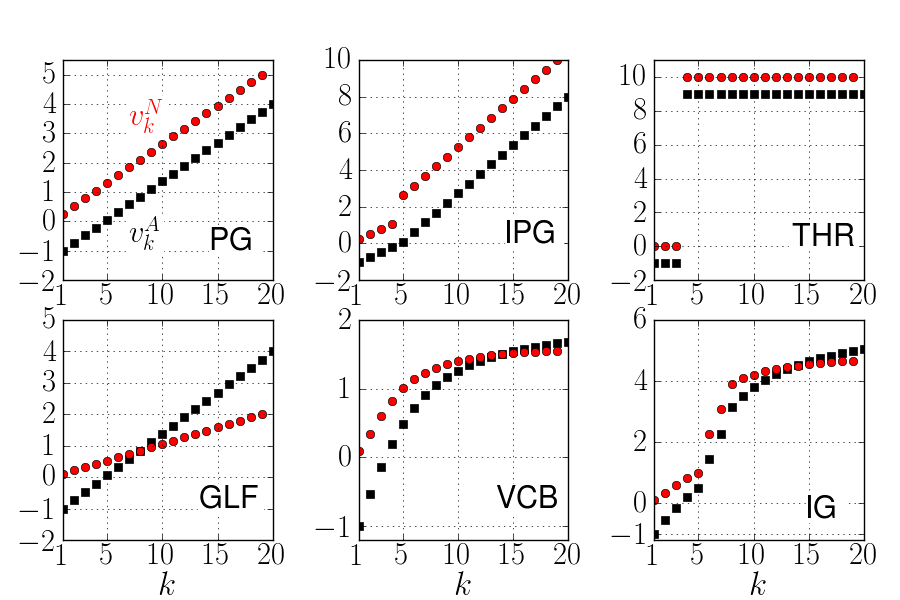
with the convention that , i.e., . The quantities and represent payoffs to altruistic, or non-altruistic behavior. The parameter indicates the strength of selection, with the limit corresponding to the limit of weak selection, and the case corresponding to the case in which there is no selection, only neutral genetic drift. Examples of payoff functions will be provided in Section 2. See also Fig. 2.
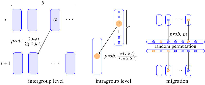
Evolution operates as the next generation is formed through a process that involves group competition and competition within groups, followed by migration at rate , as summarized in Fig.1. Competition among groups is idealized as an (intergroup-level) Fisher-Wright process with selection, described as follows. We associate to each group a relative fitness given by the average relative fitness of its members. This means that a group with altruists has relative group fitness
| (1) |
Each group in the new generation has a parental group from the previous generation, chosen independently with probability proportional to group relative fitness. Competition among members of a group is described by an (intragroup-level) Fisher-Wright process with selection, described as follows. The members of each group in the new generation each has a parent from among the individuals in their parental group, chosen independently with probability proportional to the fitnesses of the members of that parental group. (A standard probability computation, using conditioning on the parental group, shows that each individual in the old generation has then an expected number of offspring proportional to its relative fitness. Conversely, for this to be true, the fitness associated to the groups in the intergroup level Fisher-Wright process must be given by (1). The conceptual relevance of this equivalence is emphasized in [36].) Once the new groups have been formed according to this two-level Fisher-Wright process, a fraction of the individuals migrates from their group to a randomly chosen group, preserving the constancy of the number of members of the groups. More precisely, each individual, independently of anything else, leaves its group with probability ; the migrants then return to the groups in a random fashion, filling vacancies, so that each group has again members. Each possible way of assigning the migrants to the vacancies left in the groups is equally likely, meaning that the migration process is completely random. (Mathematically: each individual is independently of anything else, with probability , declared to be a migrant, and one applies then a random permutation to the set of migrants.)
In the case , we can equivalently think that the new groups are formed by random assortment from a metapopulation with individuals. Each one of these individuals has a parent chosen independently with probability proportional to relative fitness from the individuals in the old generation. This is precisely the traditional trait-group framework.
A model within our framework is specified by giving the values of and the relative fitnesses and . The number of groups will be considered to be very large, corresponding to taking the limit in the computations. The study of how finiteness of modifies the conclusions is very interesting, but will be deferred to a later investigation.
Our results on the viability of a single gene A to spread do not depend on any conditions on the parameters of the model. (These results are summarized in the paragraph that contains display (9).) But to keep the presentation more focused and interesting, we will assume that conditions (C1) and (C2) below hold, except when stated otherwise.
-
(C1) , i.e., , so that an isolated type A individual has lower fitness than the wild type N has in groups without altruists.
-
(C2) , i.e., , so that type A individuals have greater fitness when in single-type groups than type N individuals have when in single-type groups.
Condition (C1) is sometimes referred to, after [83], as the condition for A to be called “strongly altruistic”. This condition means that an isolated gene A is at a disadvantage with respect to the wild type N in the population at large. In the trait-group framework, , this condition makes it impossible for A to invade. We will see that, as expected, this condition makes it impossible for this gene to invade also when is close to 1, so that .
On the other hand, we will see that condition (C2) is sufficient for A to spread when is close to 0, so that .
We will study the evolution of the population, when started in generation 0 from the situation in which only one individual is of type A. Naturally this refers to the situation in which a mutation from N to A has just occurred, and to the assumption that the mutation rate is so low that no further mutations will occur before the fate of that mutant gene has been decided. Obviously the mutant A may disappear in a few generations, but we want to determine here when it is viable, in the sense that it has a fair chance of spreading. We will denote by the number of altruists in generation . In case , meaning that the mutation is neutral, the expected number of altruists remains constant, , and a standard martingale argument gives probability to the event that A will not disappear, but rather fixate eventually. As this probability vanishes. When , and condition (C1) holds, prospects are even worse for the mutant gene A in generation 1. The expected number of type A individuals then is . When , these bad prospects worsen with time, since in the first few generations the possible type A are likely to all be in different groups (since is large), and so are always carrying the same fitness . This leads to , and to the certain elimination of the gene A. In the opposite extreme, when , a group with altruists may be created by chance in a few generations. Groups that descend from this one will always have only type A individuals, who therefore have average fitness , by (C2). In this situation it is reasonable to expect that the altruistic gene can spread with a probability that does not vanish as . The rigorous analysis of what happens in this case and in the more important case can be done using the theory of multitype branching processes, as covered, for instance in Chapter II of [28]. We turn next to the application of that theory to solving our problem.
In applying multitype branching process theory here, we must emphasize that that theory describes well the evolution in our framework only in its early stage. By early stage, to be abbreviated E.S., we mean the generations before the number of groups that contain altruists is comparable to . We will nevertheless see that this early stage period is of order generations, so that it covers a large number of generations since is large.
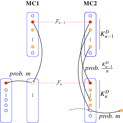
We say that a group is of type if it has exactly altruists. First we explain how multitype branching theory can be used when . In the E.S., there are few groups with altruists, compared with the total number of groups. Therefore in the intergroup Fisher-Wright process the competition among groups with altruists is basically irrelevant; groups are mostly competing with the groups without altruists, that form the background on which groups with altruists may or not spread. To see this, note first that in each generation there are new groups being formed, and that they choose their parental groups independently with probability proportional to group fitness. Since the vast majority of the groups have no altruists, and therefore group fitness , a type group has a probability close to of being the parent of each new group. Hence, each group of type , with , can be seen, in first approximation, as creating independently of the other ones a number of offspring groups that is given by a binomial distribution with parameters and (well approximated by a Poisson distribution with mean ). During the E.S., there are much less than groups with altruists, and they are each producing a number of offspring groups that is also small compared to . For this reason each one of these groups interferes little with the other groups with altruists in their creation of offspring groups. This independence in the creation of offspring groups is what defines a multitype branching process. The next fact to observe is that each group that has as its parental group a group of type will be of type , due to the intragroup Fisher-Wright process, with probability
where is a binomial random variable with attempts, each with probability of success. Assembling the pieces above, we conclude that, through the two-level Fisher-Wright process, a group of type creates in the average
| (2) |
groups of type in the next generation, independently of anything else. When this is the whole story. The matrix , of size , defined by (2), with , , characterizes the evolution of this process
When , the creation of the new generation of groups is complicated by migration. One could be concerned that a multitype branching process description is no longer feasible. Fortunately this fear is unfounded, thanks to the fact that we are only considering the E.S., during which . Altruists form then a minute fraction of the migrant population, and as a consequence it is unlikely that migrant altruists will settle in groups that contributed altruists to the migrant population, or that any group will receive more than one migrant altruist. A group that has altruists before migration, will keep after migration a random number of altruists given by a binomial distribution with attempts and probability of success. This means that the probability that after migration this group is replaced by a group with altruists is given by
| (3) |
That group that had altruists before migration, will also be contributing with an expected number of migrant altruists, who are likely each to settle in a different group that had no altruists before migration, and has exactly one altruist after migration, i.e., is now of type 1. This means that the expected number of groups of type created from groups of type 0 that received altruists from our group that had altruists before migration is given by
| (4) |
The matrix should therefore be replaced, due to migration, with the matrix in describing the expected number of groups of type created in the new generation by each group of type in the old generation. We will use the notation for the number of groups of type in generation , and also write . In summary, we have, in matrix notation, that for in the E.S.,
| (5) |
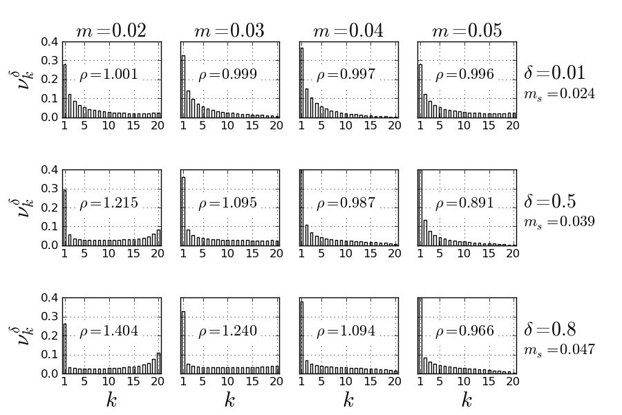
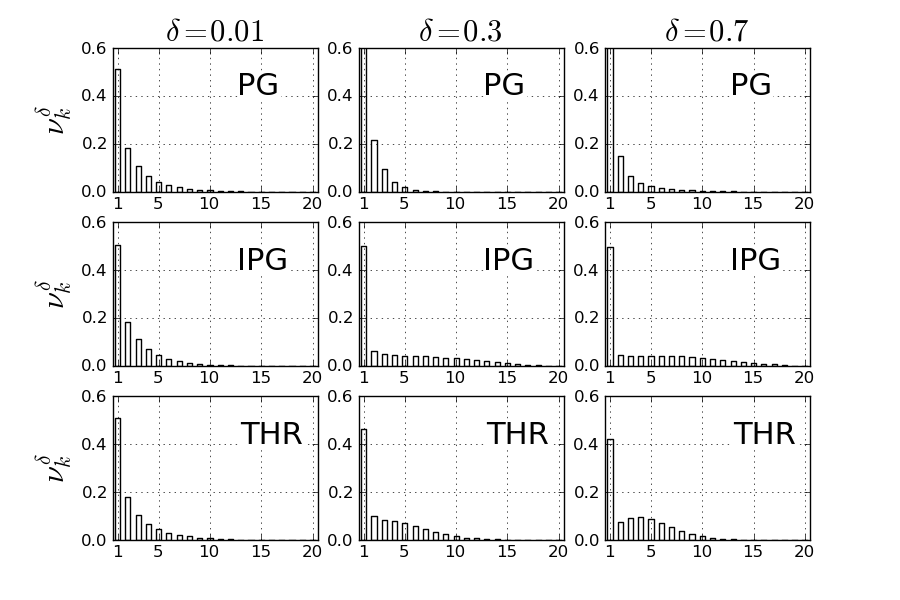
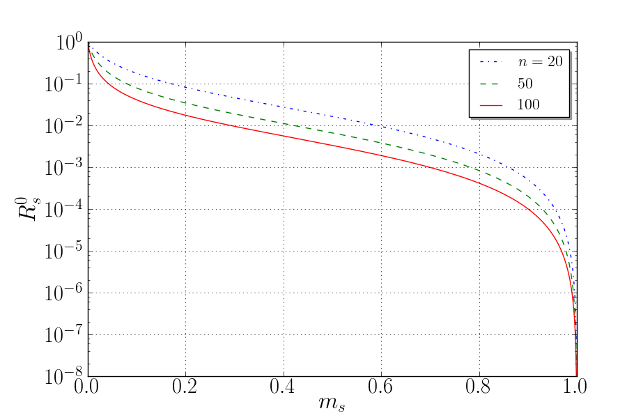
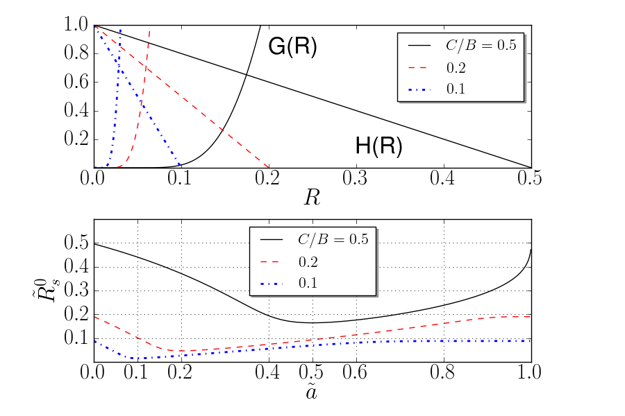
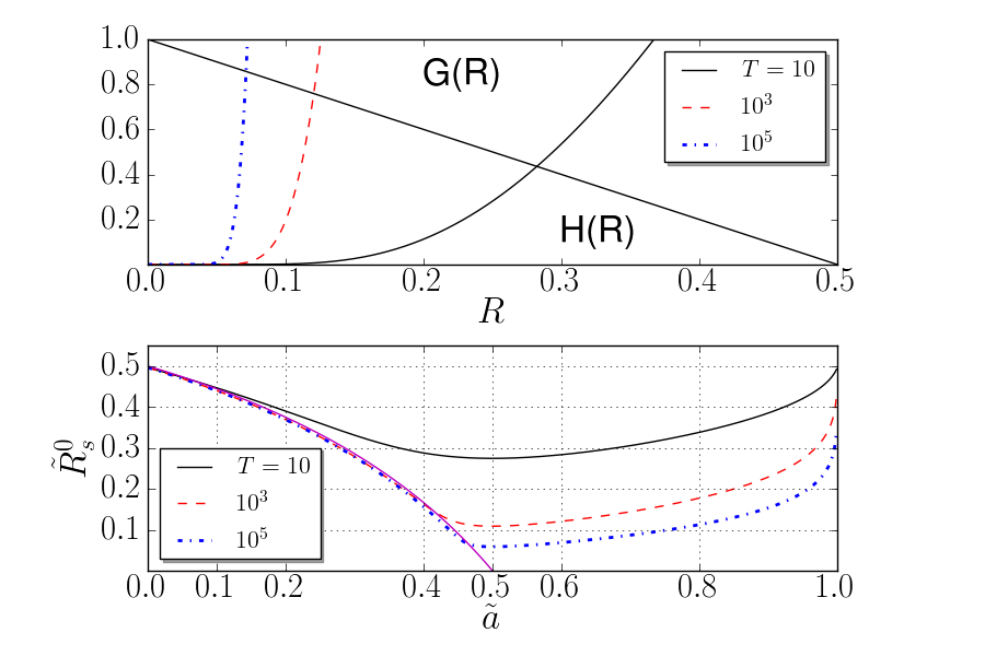
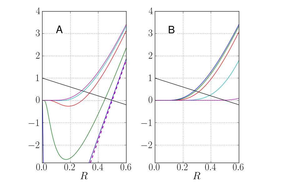
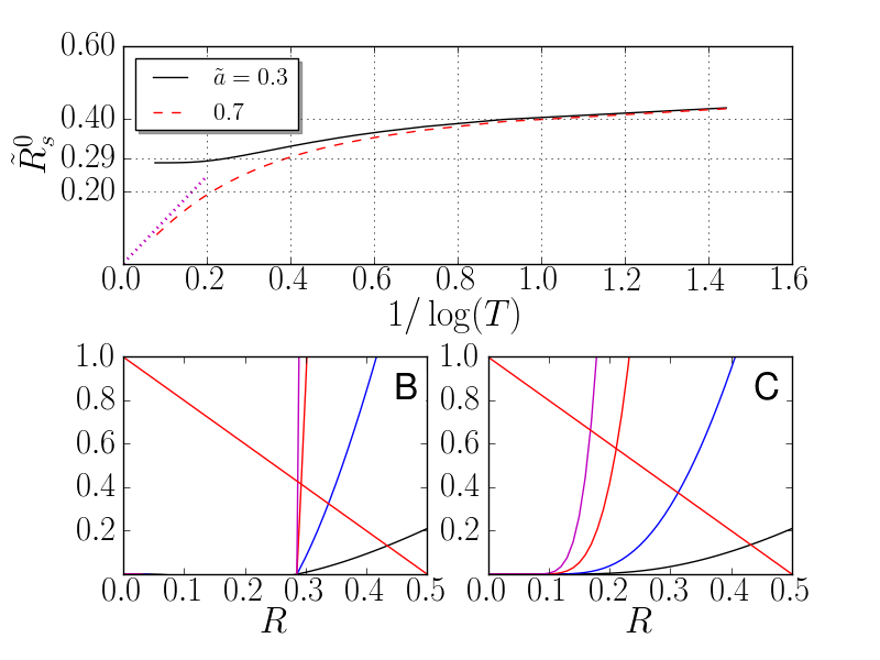
Obviously . Therefore, the survival of the altruistic gene is equivalent to the survival of the multitype branching process . Next we describe the necessary and sufficient condition for the survival with positive probability of this multitype branching process. In what follows we will suppose that ; the cases and and can be treated as limits. Because the matrix has then only strictly positive entries, it results from the Perron-Frobenius Theorem (see, e.g., Theorem 5.1 in Chapter II of [28]) that it has an eigenvalue that is simple, positive and larger in absolute value than all other eigenvalues. It corresponds to left and right eigenvectors, both of which have all their entries strictly positive. We will denote by this left-eigenvector, normalized so as to represent a probability distribution over group types: . (Illustrations of and as functions of and appear in Fig. 3, Fig. 5 and Fig. 8, for various models.) A consequence of (5) and of the Perron-Frobenius Theorem is that for large, but still in the E.S.,
| (6) |
where is a constant.
Theorem 7.1 in Chapter II of [28] states that the survival with positive probability of the multitype branching process is equivalent to the condition
| (7) |
(We will make , , etc, explicit in the notation , , etc, only when important.) The critical value is then obtained by solving the equation
| (8) |
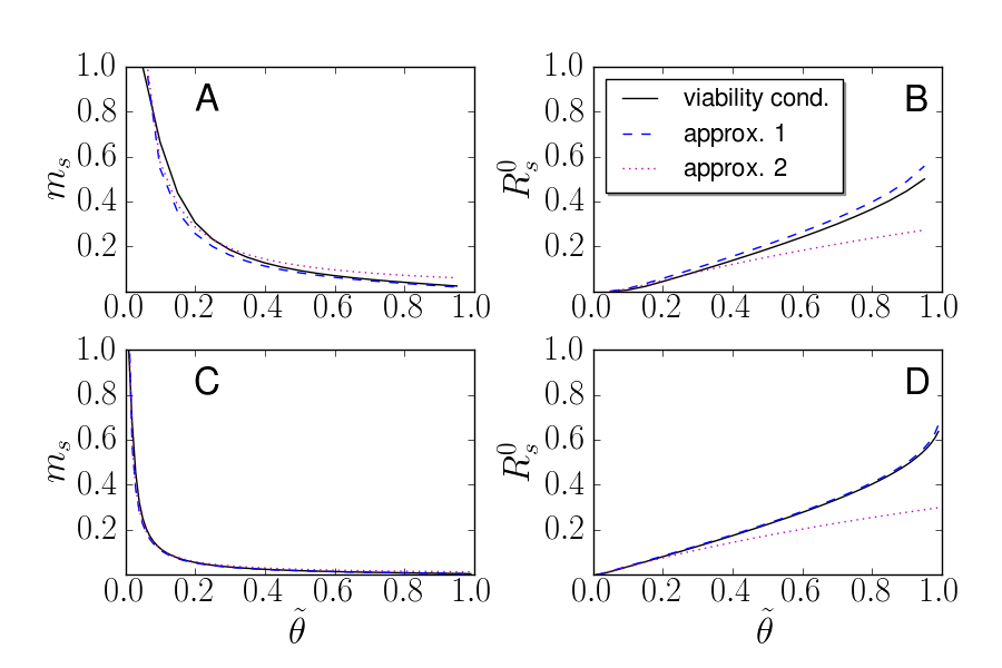
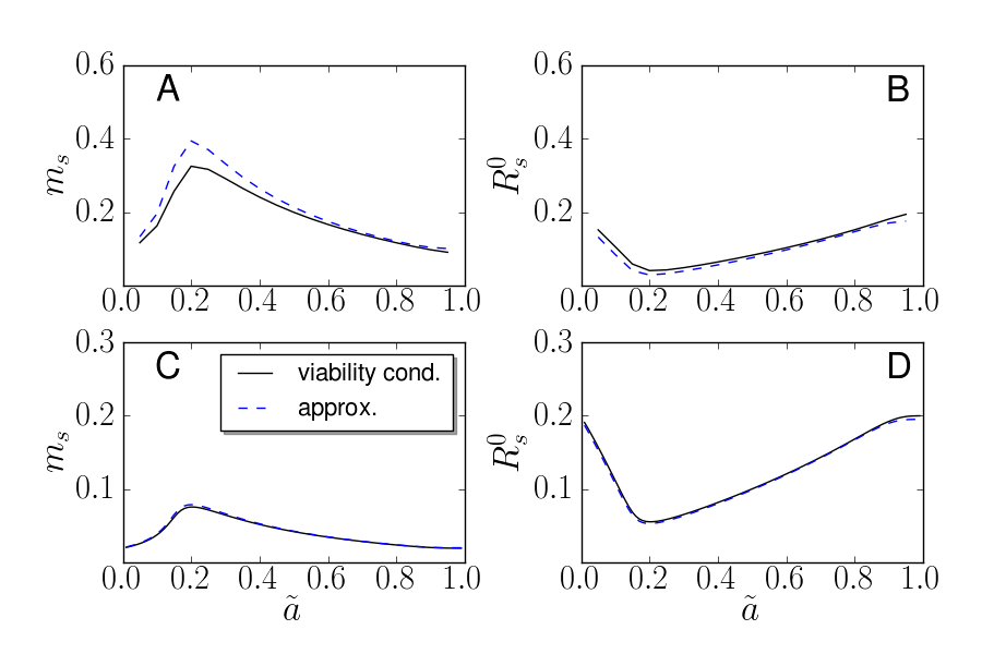
(For some numerical examples, see Fig. 3, Fig. 4, Fig. 6 and Fig. 7.) To see that this equation has a solution in the open interval , we use continuity of eigenvalues and eigenvectors. In particular is continuous, and it is enough to observe how it behaves as approaches or . When , has the eigenvalue (by (C2)), corresponding to the left-eigenvector . This implies that must be larger than 1 when is close to 0. When , the matrix , and has only the first column not identically 0. Therefore any of its left-eigenvectors must be of the form . When such a vector is multiplied by , the result is . This shows that is the only eigenvalue of . Therefore must converge to (by (C1)), as .
The argument above shows that (8) has a solution. Uniqueness of this solution is not guaranteed, unless additional conditions are assumed on the fitnesses. In any case, if there is more than one solution to (8), the natural definition of , that we adopt, is as the largest one, representing the least strength of assortment of altruists that suffices to allow altruism to survive.
The theory of multitype branching processes provides us with further detailed information on the patterns of evolution, when the altruistic gene A survives. Theorem 9.2 of Chapter II of [28] shows that in the event that the process survives, it behaves in a rather regular fashion: as becomes large, the vector tends to become a multiple of , and to grow at rate . (More precisely, the distribution of the random vector converges to , where is a random variable.) Intuitively, this is a sort of law of large numbers: if the multitype branching process survives, the relative frequency of groups of each type tends to stabilize, as that given by the vector , as becomes large. But randomness in the values of ,…, persist (and are given by the one dimensional above), due to the randomness that affects the process in the first few generations, before large number phenomena can take place.
We summarize now what we have learned about the evolution of the gene A in our framework. When (7) fails this gene dies out in a few generations. On the other hand, when (7) holds, the picture of its evolution is a dichotomy. Either A is eliminated in a few generations, or else it survives and, as it spreads, its distribution stabilizes dynamically, in the sense that
| (9) |
when . We will refer to this time period as the stationary early stage, abbreviated S.E.S.. Note that the upper bound on the magnitude of is equivalent to the condition that during this period . The condition is then what defines the E.S., and we will refer to the first few generations, before the S.E.S., as the very early stage, abbreviated V.E.S.. During the V.E.S., evolves very randomly, displaying little regularity, since the number of copies of the gene A is small. The random variable reflects how randomness during that period affects the later S.E.S., and the extent to which it is not washed out as the number of copies of A grows and the evolution becomes more regular.
Finally, the later period when is no longer negligible as compared to (provided that A has survived) will be called late stage, abbreviated L.S.. The evolution of during the L.S. will no longer be well approximated by the multitype branching process, and is more challenging to study. To focus in the current paper only on the issue of survival of the gene A, we will postpone our analysis of that problem to a later publication ([60]). Here we only observe that in that regime, laws of large numbers allows us to well describe the evolution as a dynamical system (in dimensions, representing the fractions of groups of each type). That dynamical system turns out to be non-linear (due to migration) and to sometimes have more than one stable equilibrium. Nevertheless, under the condition that (C2) holds and is small, or some alternative conditions (for instance (C3) in the next section), when is small, it has a single stable equilibrium, corresponding to fixation of the gene A in the population. This is what characterizes the critical point . It is worthwhile to stress in this connection that the linearity of the evolution during the E.S., as given by (5), in spite of migration, makes the issue of deciding when the mutant A can survive much easier than it would be otherwise. This is what allows the reduction of the problem to a standard eigenvalue problem.
Returning to our analysis of the E.S., We can see (9) as a form of self-organization of the gene A. If it survives, it arranges itself according to the distribution , that is a left-eigenvector of the driving matrix . Left-eigenvectors are precisely the arrangements that the process can have which are preserved in time. To better appreciate what is special about , and for several future uses, we observe that if is a left-eigenvector of , with eigenvalue , and no negative entries, then
| (10) |
In other words, is the average fitness of the individuals who carry the gene A (or simply, the average fitness of the gene A), when the groups with altruists are distributed according to . Identity (10) is an easy consequence of two observations. First that from (5) we know that if for some constant , then . This implies that . Second, that in the multitype branching process an individual who carries the gene A and belongs to a group with altruists produces an expected number of offspring , so that we can also write . Comparison of these expressions yields (10).
We combine (7) with (10) to write the necessary and sufficient condition for viability of the gene A as
| (11) |
Since is the only left-eigenvector of the maximal eigenvalue , (9) is telling us that when the altruistic gene survives, it tends to organize itself (or we can also say “nature organizes it, through natural selection”) in the stable way that maximizes its average fitness. This observation also makes the condition of survival (11) look particularly natural. If , there is no stable way for the gene A to be organized so that it will have an average fitness that is larger than that of the wild type N in the population at large, where A is still rare; A will then not be viable. On the other hand, when , the gene A can be organized according to , that is stable, and provides it with mean fitness larger than 1, as needed for it to spread among the wild type N.
It is enlightening to see what happens when the inequality in (11) fails. Even in this case, chance may produce at a time during the V.E.S. the arrangement , meaning that there are exactly altruists, all in the same group. Condition (C2) tells us that at time the average fitness of the gene A is larger than 1. And indeed, , so that the altruistic gene is spreading at this time. But this arrangement is not stable. In successive generations, the distribution of is driven to a combination of left-eigenvalues of , and can grow then at most at rate , so that eventually it is eliminated.
In contrast, when (11) holds, chance will dictate if during the V.E.S. an arrangement of copies of A will form that not only provides that gene with mean fitness larger than 1, but is also likely to produce a succession of arrangements in the next generations, all with this property. The important point is that, under (11), such arrangements do exist, and drive the evolution towards .
The contrast in the last two paragraphs is one of the main lessons from our analysis. This lesson goes beyond the specific aspects of the stylization that we are adopting here. We suggest making this idea explicit as a guiding criterion, that should be of use when considering any framework, model or experimental situation.
Viability or Survivability Criterion: In a large population, a single mutant gene A, in the absence of further mutations, will be viable, i.e., will have a positive probability of surviving and spreading, if and only if this gene can produce in a few generations an arrangement of its copies in a number that is still small compared to the size of the population, but is likely to produce in the next generations a sequence of arrangements with a growing number of its copies, until it accounts for a non-negligible fraction of the alleles in the population.
We will refer to such a sequence of arrangements as a survival mechanism for the mutant gene A, so that the criterion stated above postulates the existence of a survival mechanism as a necessary and sufficient condition for the viability of the mutant gene A. Such a mechanism can, for instance, be started by an arrangement of copies of the gene A that satisfied the three conditions below:
-
(i) When in this arrangement the average fitness of the mutant gene is larger than that of the wild type in the population at large, before the mutant appeared.
-
(ii) This arrangement is likely to produce in the next generation another arrangement with the same property (i) above.
-
(iii) Due to the growth in the number of copies of the gene, the probability of success in step (ii) above increases from generation to generation, fast enough to assure that the probability of producing the sequence of arrangements mentioned in the criterion is large.
Indeed, in our framework, once an arrangement of copies of A is produced with distribution in groups close to , conditions (i), (ii), (iii) are fulfilled, provided that . On the other hand, when , no arrangement exists that satisfies these three conditions.
We end this section with some observations on generalizations of our methods. One can modify the intergroup and the intragroup competition procedures, from the Fisher-Wright ones that we consider here, and in this way extend our framework further. For instance, modifications to the intragroup selection procedure can be fairly general, and would only require a modification of the matrix . Instances of such a modification could include domination patterns in the intragroup reproduction mechanism, that result in reproductive skew within the group. In an extreme case, a single member of the group, chosen at random with probabilities proportional to individual fitness of the group members, could mother all the offspring of an offspring group.
Modifications of the intergroup competition mechanism are even simpler to consider. Note that we did not use in our analysis the full power of the assumption that this mechanism is a Fisher-Wright procedure. We only assumed that if altruists are rare, then groups with altruists father each in the next generation an almost independent random number of groups, with mean proportional to group fitness (defined as average fitness of group members). Under these broad assumptions our methods and results above, and in the remainder of this paper, are unchanged. We chose to introduce our framework with a Fisher-Wright competition mechanism among groups for concreteness. This choice forces the number of offspring groups of each group to be binomially distributed (well approximated by Poisson, since is large). The observation in the current paragraph is of special relevance then in situations in which the number of groups fathered by each group is better modeled by a distribution that is far from Poisson, as for instance in cases in which their variance is much smaller than their mean (as happens, for example, when is small, the mean is close to 1, and the variance is much smaller than 1, with most groups fathering exactly one group).
2 Models
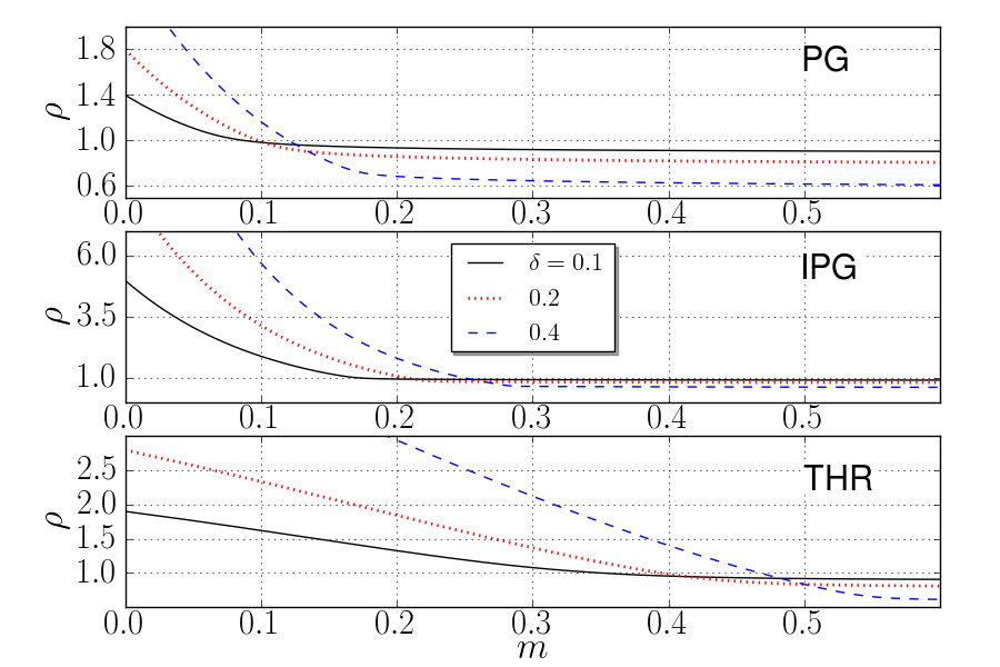
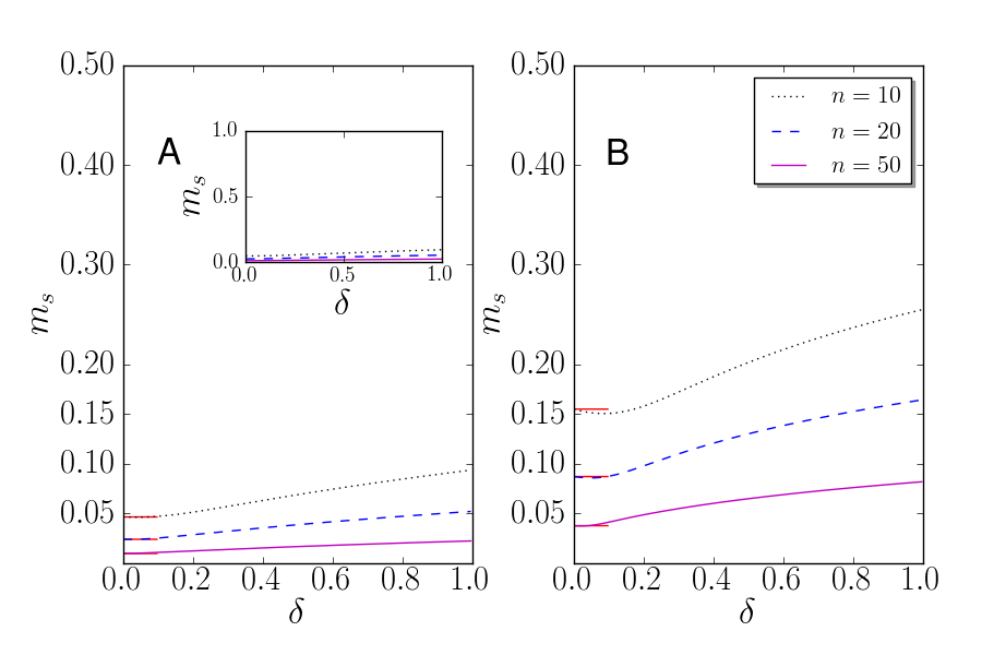
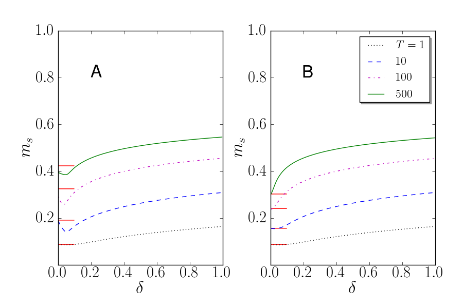
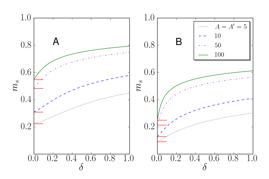
In this section we will introduce several models and discuss their relevance. Fig. 2 provides an overview of some of their typical features. Fig. 4, Fig. 6 and Fig. 7 provide values of as function of the strength of selection for some of them. Notice, from these figures, that is not always monotone in , but that it often increases substantially when is large. This fact highlights the relevance of studying the models not only when selection is weak. Notice also that in Fig. 6 and Fig. 7, the product can be of the order of . This is relevant in view of the widespread claim that altruism cannot survive when is significantly larger than . As far as we know, this perception resulted from the analysis of particular models (e.g., in [43], [2] and [10]) and an excessive emphasis on the public goods game (Example 1, below). One of the main messages from this section and the following ones will, indeed, be that mechanisms that go beyond the public goods game may be central to the understanding of the spread of altruistic genes, and can be analyzed in our framework with no special difficulty.
Conditions (C1) and (C2) are very mild, and basically characterize the effect of the gene A on its carriers as an individually beneficial social effect which comes with a personal cost to them. One does not have to restrict oneself to behavioral effects of the gene A on its carriers phenotype. For example, another kind of application could include anatomic and physiologic effects that carry a cost, but produce benefits to those with the altered phenotype when in groups with others that share this feature. For instance, gene A could promote changes that facilitate verbal communication with others that have the same changes, but at a cost, say, in adding expensive tissue to the brain. An isolated carrier of gene A would suffer the costs of carrying it, but without the possibility of benefiting from its potential advantages.
In order to assure , in a forthcoming paper ([60]), we will either have to assume that in addition to (C2) holding, is small, or else we will need to add an additional assumption. A sufficient one will be:
-
(C3) , i.e., , for , so that the average fitness of a group is maximized when the group contains only altruists.
When the gene A affects behavior, what precise conditions on the fitnesses and should be required for this gene to be called “altruistic”? There is no agreement on the answer. The issues are very nicely presented and discussed in [37]. We list next a few of the conditions that can naturally be associated with altruism. These ones, and a few more can be found in [37], where detailed references and credit are given.
Some of the conditions require the altruistic behavior to be beneficial. Typical conditions of this kind are:
-
(C4) , or equivalently, , is increasing in , so that altruists are always better off sharing their group with more altruists.
-
(C5) , or equivalently, , is increasing in , so that non-altruists are always better off sharing their group with more altruists.
-
(C6) , or equivalently, , is increasing in , so that the members of a group are in the average better off with more altruists in the group. (Note that (C6) is an extension of (C3).)
And complementary conditions require the altruistic behavior to come at a cost to the actor:
-
(C7) , i.e., , , so that altruists are always worse off than non-altruists in the same group.
-
(C8) , i.e., , , so that an individual that suffered a mutation from N to A, would be worse off.
Condition (C8) extends condition (C1). It is known that when it holds, then in the trait-group framework, , starting from any fraction of genes A in the population, these genes will be eliminated. ([37] attributes this result to [45].) The assortment provided by a low is nevertheless sufficient to allow a single altruistic gene A to invade, if condition (C2) holds.
We will illustrate the use of our framework with several examples (see Fig.2):
Example 1. Public goods game:
for positive constants and . One can think that at a cost to itself, each altruist provides a benefit to each one of the other members of its group. Alternatively, one can think that at a cost to itself, each altruist provides a benefit to each member of its group, itself included. Set then , for the net cost to the altruist, and , for the total benefit to the other members of the group. Each one of these two descriptions is common in nature, has its theoretical advantages and both appear often in the literature (see [55] for more on this point). The former description is often referred to as “other-only” trait, and the latter one is then referred to as “whole-group” trait. Their mathematical equivalence illustrates something that presents itself a number of times. Two models may be different in relevant biologic aspects, but lead to the same functions and , possibly after some change of variables, as above. In this case, we will say that the models are materially different, but formally equivalent.
There is a second way in which the present example splits into two materially different, but formally equivalent descriptions. On one hand, altruists could be performing individual actions, producing identical benefits to all the other (or to all, self included) members of the group. In some applications this may be a good description of what is happening. For instance, altruists could be individuals with a hygiene habit that is beneficial to the group, in preventing disease, but costly to the actor. Alarm calls are another example.
On the other hand, the fitness functions in this example can also accommodate collective actions, in which altruists act together, to produce a common good for the group. Fighting in a war against another group, or participating in collective hunting activities (with the product of the hunt shared among all members of the group) would be examples of this kind.
In all cases, the assumptions that the total benefit produced, , grows linearly with the number of actors, and the net cost to each actor, , is constant, may be unrealistic. We will explore these points in Example 5, below.
Note that . Condition (C1) holds since . We suppose that , so that (C2) holds, since . Note that then also (C3)-(C8) all hold.
The public goods game has rightfully been called “the mother of all cooperative models” (see footnote 1 in [70]). It is natural to study its behavior, and to understand how the gene A can spread in this case. In the next examples we will nevertheless try to convey the message that one should aim at developing methods, as we do here, that can address more general models, as well. In the spirit of that metaphor, it is natural to see the next example as “a special daughter of the public goods game. It derives from the public goods game in the same way that (in a two player setting) the iterated prisoner dilemma and the tit-for-tat strategy derive from a one shot prisoner dilemma game and a simple cooperative strategy.
Example 2. Iterated public goods game. Altruists cooperate conditionally:
for positive constants and , and . Here we suppose that a public goods game is repeated a random number of times , with average . Each time each member of the group can cooperate at a cost to itself, resulting in a benefit to each one of the other members of its group. Defectors incur no costs and produce no benefits. We suppose that altruists cooperate in the first round, and afterwards only cooperate if at least other members of the group cooperated in the previous round. This is a generalization of the well known tit-for-tat strategy, which corresponds to the case , . We will refer to the strategy of the altruists in this example then as “many-individuals-tit-for-tat (with threshold )”.
Note that when , regardless of the value of , this example is identical to Example 1. Note also that if , and if . Again, we suppose that , and so both, (C1) and (C2) hold, since and . It is also easy to see that then (C3), (C5), (C6) and (C7) hold.
Condition (C4) will only hold under additional assumptions. A very natural one, that we will assume, unless stated otherwise, is that the threshold satisfies
| (14) |
i.e., when altruists keep playing the game, it is never in their disadvantage to do so.
It is instructive to look into what happens with (C8) in detail: , if ; if ; but in the case , . Therefore, if (14) holds as a strict inequality, then , for large , and (C8) fails. But if (14) fails, or holds as an equality, then (C8) holds, for arbitrary . Note that if (14) holds as an equality (which can only occur if is an integer), then all the conditions (C1)-(C8) are satisfied.
This model was studied independently in [7] and in [32], in the trait-group framework. Both papers identified stable equilibria with positive fractions of altruists (a phenomenon that can occur only when (C8) fails). But they also observed that altruists could not invade when rare (a phenomenon that always holds under (C1)). In [7] an approach was then introduced to provide assortment and allow the gene A to invade when rare. The authors concluded that such invasion by gene A could only occur under very restrictive conditions, and that therefore this model and the corresponding notion of many-individuals-tit-for-tat were of marginal relevance. One of our contributions in the current paper is to rectify this perception. In our framework, we obtain values on large enough to indicate that this model should be seriously considered as a possible mechanism for the spread of altruistic genes (see Fig. 6 and Fig 15). Indeed we will see that the estimates in [7] contained an unreasonably pessimistic assumption, that is not supported in our framework (see last paragraph in Section 5).
From a theoretical point of view, this model is still mathematically simple enough to lead to an interesting detailed analysis of the conditions under which the gene A can spread, in case selection is weak and the group size is large, with the threshold proportional to . This analysis (illustrated in Fig. 16, Fig. 17, Fig. 18, Fig. 19 and Fig. 20) will be a good illustration of the simplifications that will be obtained, in Section 5, in that regime.
We see this example as the prototype for an important class of models, that we make explicit in Example 6 below, and that we believe should be seriously considered and studied.
Example 3. Threshold model:
for positive constants , and , and an integer . The idea here is simple: the gene A carries a cost, but allows its carriers to gain benefits if sufficiently many are in the group. Non-altruists obtain benefits also when altruists do, but we allowed for the possibility that those are smaller or larger than those of the altruists.
This model may be seen as a simplification of Example 2. It shares with it the features that when few altruists are present, they incur costs, but when in numbers larger than a threshold, have positive payoffs that may be much larger than those costs. The fitnesses in this model are sufficiently simpler than those in Example 2, to allow for a more transparent analysis of its behavior. We will see that this model is of great value when we discuss conceptual issues, including Hamilton’s rule. In [70], the case of this model (called there “stag hunt game”) was discussed in connection to the conceptual issue of the role of Hamilton’s rule. This raised a debate in [44] and [71] and further analysis in [20]. We will comment on this at the end of Section 3.
Example 3 is also of great value for comparison purposes, providing meaningful bounds on the behavior of more elaborate and realistic models. For instance, the very elaborate fitness functions studied in [6] are well approximated by those in Example 3. We are currently reanalyzing the work and ideas from [6] in the context of our framework, and taking advantage of this relationship in that project ([61]).
This model can also be seen as a simple instance of another natural class of models that we introduce below, in Example 5.
If , then either (C1) or (C2) is violated, since then . So we suppose that . Under this assumption, (C1) is immediate from , and we suppose that , so that (C2) is also satisfied. Conditions (C4) and (C5) are clearly satisfied then. Condition (C7) will be satisfied in case . We have , if , and , if . So (C3) (and therefore also (C6)) may not be satisfied. (C3) holds, nevertheless, if . (But even under this assumption, (C6) fails, unless .) As for (C8), it fails, regardless of the value of , in the same fashion that it failed (in general) in Example 2, since .
Numerical results for Example 3 appear in Fig. 7, Fig. 8 and Fig. 14). As with Example 2, Example 3 also nice illustrates the simplifications that will be obtained, in Section 5, when is small and is large (see (61) and (62)).
Example 4. Additive pairwise interactions (general linear fitness functions):
Here we suppose that members of the group interact in a pairwise manner throughout their lives. Each such pair interaction contributes a certain amount to the total payoff of each one of the two individuals. The contribution from each pairwise interaction to each one of the two participants depends only on their types. The payoff to a type interacting with a type will be denoted , = A,N. In addition, each individual has a self contribution, to its payoff that depends only on its type = A,N. These contributions are added to produce the final payoff. The result is displayed above, and then rewritten in terms of , , , where we incorporated the assumption that
This assumption carries no loss of generality, since a constant can be added to all the payoffs and without modifying the behavior of our process. (The behavior of the process is clearly not modified by multiplying all fitnesses, , , by the same constant. If we add a constant to all the payoff functions , , the new fitnesses are equivalent in this sense to the old fitnesses with replaced by .) This condition amounts simply to our convention that . Expressing the fitness functions in terms of , and , makes their relationship with Example 1 and Example 5 below easy to see. Finally the result is also rewritten in an equivalent form that emphasizes the nature of the dependence of the fitnesses on : they are linear functions. Here , and .
An important point to make is that given linear fitness functions and , with , as above, they can always be represented in the other two ways, with an appropriate choice of the constants. For instance, we can take , and , and then take , , , .
When , the current example is the most general possible choice of the payoff functions and . But this is obviously not the case when . For each value of , the most general form of the payoff functions are polynomials of degree .
The linearity of the functions and will play important roles in relating our results to other concepts, especially Hamilton’s rule. This is one of the reasons this is a major class of models. The mathematical equivalence between these linearities and having pairwise additive interactions should not confuse one into thinking that the linearities imply that the fitnesses must indeed have originated from that special kind of interaction. In Example 1, the members of a group may be interacting in a collective way (hunting together, warfare, etc). All that the mathematical equivalence says is that the fitnesses obtained there, are the same ones of a, ficticious in this case, pairwise interaction scenario. This is a good illustration of two formally equivalent, but materially different models.
There are realistic stories that are conceptually associated to the public goods game, Example 1, but lead to the more general payoff in the current example, with . For instance, the altruistic activity could be hunting more dangerous but also more nutritional prey. If the products of the hunts are always shared by the group, we have the model in Example 1. But if the hunters are able to consume the best part of the hunt, before sharing the rest with the group, we would have .
While materially different from the public goods game, Example 1, the current example is formally equivalent to it when the following equivalent conditions hold:
| (17) |
Condition (17) is know as “equal gains from switching”, since the payoffs in the matrix , A, N, change by the same amounts if one switches strategies, regardless of what the other player is doing. Unfortunately the terminology “additivity condition” or “linearity condition” is also used in the literature for (17). This is confusing, since in our context, additivity refers to the fact that the payoffs and are obtained additively over the pairwise interactions that each individual has with the other members of its group. This additivity has no relationship with (17). And in our context, linearity, refers to the linearity of and as functions of . As we explained above, in the mathematically standard way in which we are using the terms pairwise additivity and linearity, they are equivalent to each other, and logically independent of (17).
Under condition (17), it is common to use the representation , , , . When , this is a classical prisoner’s dilemma. It corresponds to , .
The matrix represents the lifetime payoff for each pairwise interaction. This lifetime payoff may result from the accumulation of payoffs from iterated games. In this way we can see that the setup in this example is flexible enough to accommodate a gene A that produces a conditional behavior over such iterated games, like, for instance a tit-for-tat strategy. For this, suppose that each pair of individuals interact repeatedly with payoffs given by the standard prisoner’s dilemma matrix. If type N always defects, and type A uses a tit-for-tat strategy, we have , , , , where is the average number of repetitions of the basic interaction over a lifetime. If , (17) fails, and we have
| (18) |
It is common to write and call it a “synergy” term. It represents an additional benefit (possibly negative) to altruists when interacting with other altruists. In the iterated pairwise prisoner dilemma game with A playing tit-for-tat, (18), we have .
Deciding when each one of the conditions (C1)-(C8) holds in the current example is tedious and not so relevant. We observe only a few facts. Assuming s (C1), (C2) and (C4), that only depend on . If , then also (C5) holds. The other conditions depend on how relates to and . We just make the simple remark that if and is close enough to , then all the conditions (C1)-(C8) hold, since they hold with slack when (Example 1).
In Example 1, we observed that the assumed linearity of and there may not be realistic. The same observation holds about pairwise additivity of interactions. Many interactions in a group are between pairs, but it is not always clear that their effects on fitness should be additive. When an individual interacts repeatedly with another member of the group, like in the story that lead to (18), it may not be able to interact as often with the other members of the group. Also, the beneficial effects of the pairwise interactions may saturate, and be sub-additive, rather than additive. Additivity/linearity is mathematically a natural first level simplification/approximation. But one should be aware of its limitations. With this in mind, we turn to the next example.
Example 5. Variable costs and benefits:
Remarks in Example 1 and 4, above, motivate this class of of examples. Without further assumptions on the costs and benefits functions, , and , any model can be fit into this form. So that what we are proposing here is first a convenient notation for comparing models. Next we discuss some interesting assumptions on the costs and benefits functions.
It is very natural, in various applications, to assume that is non-increasing and and are non-decreasing. If the gene A prompts its carriers to act in some collective way, it is often the case that the cost to each participant decreases with the number of participants, while the total benefits produced grow faster than linearly with the number of participants. This is called an increasing return to scale. Reasonable assumptions can be that decrease as a power of , , for some constant , while and , with , , , .
Another distinct assumption on the benefit functions is that and first grow slowly with , then steeply (close to a threshold value of ) and then more slowly again, as the gains from scale saturate. For instance this will happen if , , with positive constants , , , .
An interesting class of models covered by the current example is the object of [29]. Experimental results with microbes often indicate the need to consider non-linear payoff functions, as those discussed in the current example; see, for instance [8] and [63].
In case of a collective action that requires a minimum number of participants, we should have , for . And for larger values of , and should grow, but again typically not linearly. For instance, gene A could promote a behavior that can only be implemented in groups of at least 4 individuals, say. This could be a type of large game hunt, that requires 4 hunters. Gene A causes changes to the individual’s phenotype that make this kind of hunt possible, but at the expense of adding expensive muscular and/or brain tissue. Types N just hunt individually small game. We suppose that the hunters share their product with the group, and that large game produces greater benefits per person in the group, than small game hunt. How will and grow when ? The answer will depend on ecological conditions, and detailed aspects of the hunting technique. Can several different groups hunt simultaneously? Would the hunt be more efficient with 7 hunters than with 4? If most group members are hunting large game, would the productivity of small game hunt increase so as to make it advantageous for the group to combine both types of hunt? And so on.
Example 6. Iterated game. Altruists cooperate conditionally, based on feedback:
Here can be seen as an average number of repetitions of a basic activity. This class of models builds on the models in Example 5 in a fashion that generalizes the way Example 2 was built on Example 1. We are supposing that a certain activity presets itself to the group periodically. The output each time depends on the behavior of the group members, and gene A modifies this behavior. Carriers of gene A behave first in a way that is beneficial to the group. And afterwards, they will or not continue acting in this way, depending on feedback that they receive. For instance, if the activity is a type of collective hunt, they will have feedback as they consume the product of the hunt. In Example 2, the feedback was a count of the number of participants, and this is also a possibility, but not the only one. In Example 2, was a step function, jumping from to , at . But it seems also natural to consider smoother functions , that increase first slowly, then steeply, and then saturate. This could result from the fact that the feedback, from each repetition of the activity, is subject to random noise, and only gives clear cues to the altruists, outside of a critical window of values of . For values of in the critical window, altruists may repeat the activity a few times, before deciding to stop participating.
Models represented in Example 5, with non-increasing and non-decreasing , have a natural threshold value of , where their payoff to altruists becomes positive. In Example 1, this threshold value , corresponds to the condition (14) that appears then in Example 2. If the feedback that affects the willingness of altruist to continue participating in the activities promotes a function that (as in Example 2, with assumption (14)) starts growing above that threshold, the resulting behavior becomes more adaptive than it would be without feedback effect.
Mathematically the models in the current example can be incorporated in Example 5, by modifying the definition of , and . But the point of the current example is to provide justification for, and a mechanism behind, a class of models in which as increases, switches from small negative values to much larger positive values after a threshold value of is crossed. These models can be approximated by and/or compared to the simple case given in Example 3. It then becomes natural to analyze that model with ratios which can be as large as 100, or 1000. For instance, suppose the species under consideration to be early humans, with an adult reproductive lifespan of over 20 years. If the activity in consideration is repeated with a frequency of 50 per year, and if with negative feedback altruists stop participating after about 10 repetitions, then we can consider a factor of between with large and with small .
Obviously the perceived feedback cannot be the payoff in the model, which is related to expected number of offspring in the future. But it is sufficient that the feedback be strongly correlated with this payoff. This is not a special problem about altruism, when behavior is mediated by feedback, natural selection will align reaction to feedback with fitness.
The combination of increasing returns to scale, with the possibility of only pursuing the behavior when it is advantageous to the actors, due to a high level of collective participation, may have been a powerful set of mechanisms that led to the evolution of altruistic and cooperative social traits. This idea has, for instance, been explored in [6], where a model of that nature was analyzed in connection with the trait of punishing, at a cost, those that do not cooperate with the group. In that model, types A produce first a costly signal announcing that they are willing to participate in costly punishment. But they only implement the punishment if a sufficiently large number of group members signaled their willingness of doing it too.
Another story that fits with increased returns to scale, modified by feedback induced discontinuation, can be suggested for the emergence of “compassionate feelings” for group members. A gene that promotes those emotions, would cause their carriers to help fellow group members in need, at a cost to themselves. While there are few group members carrying this gene, they will not be able to do much for all those that may need help, in a large group. Feedback, in the form of frustration for not being able to help as they want, may lead them to discontinue their helping activities, in a short while. But with enough carriers of that gene in a group, they become able to successfully provide help to all that need it. Under this condition they pursue this activity, throught their lives. At the same time, under this conditions, the altruists themselves have their fitnesses increased substantially, from living in a helping environment. This suggests that this story may be represented by a payoff function of the type that we are introducing in the current example, with that can reasonably be taken to vary by a factor of 100 or more, as a threshold window is crossed.
3 Conceptual discussion
We start next on a long conceptual discussion of our results, and how they may help clarify some controversial issues related to the emergence of altruism through natural selection.
First we consider how our results and the underlying mechanisms revealed by them relate to “group selection”, “multi-level selection” and “kin selection”. This is not the place, and neither do we have the expertise to discuss in detail the various nuances of the semantics involved in these questions. But a few words are in order, and should be of value to the readers.
The use of the expression “group selection” has changed over the years, and is still somewhat controversial. Nevertheless it seems to us that under any reasonable use of that expression, group selection is an important force operating in our setting. In our framework, individuals belong to groups, groups compete among themselves, and in this way the fitness of individuals depends on the constitution of their groups. In our typical examples, the fitness of each altruist is strictly smaller than the fitness of the non-altruists in its group (Condition (C7)). It is only through the higher fitness of groups with many altruists, that the altruistic gene A is then able to survive and spread. Individuals also compete for reproduction with other members of their own group, so that in our setting group selection is one of the components of a “multi-level selection” process.
Is the mechanism of kin selection present when the mutant A spreads? We understand kin selection as a process in which copies of a gene, originating from a recent common ancestor, interact with each other providing themselves with an average fitness large enough for this gene to survive and spread. This is precisely what happens in our case, and is also what we tried to capture in more detail in the viability criterion and associated survival mechanism presented at the end of Section 1. In other cases, the assortment and organization of the genes could be caused by kin recognition. In our case it is caused by viscosity, that results from the group structure of the population and limited migration. In a model in which an isolated mutant has relative fitness lower than the wild type (condition (C1) in our case), its only hope for survival is in the creation by chance of a few of its copies, that happen to be so arranged that they have higher average fitness than the wild type in the population at large, and for the structure of the population to be such that this gene can then spread by what we called survival mechanism.
In this connection, condition (11) can be seen as providing a “gene’s eye view” of viability in our setting. As noted above, the left hand side in this condition is simply the average fitness of the gene, when it is arranged in the best possible stable way, to assure its spreading. It is common to refer to the average fitness of a gene A as its neighbor modulated fitness. Under certain conditions it is known that the neighbor modulated fitness can be computed also as an “inclusive fitness”, in which one adds the effects of a randomly selected gene A from the population on the other genes A. At this point, we are not sure how far this method can be extended. (See [24] for a general investigation of this question.) We will address later in this paper the issue of the validity of the related Hamilton rule in our setting, but we will defer the answer to the question of when the neighbor modulated fitness of the gene A can also be computed as an inclusive fitness to a later investigation.
It is worth also clarifying that in our view multi-level selection and kin selection are not the same concept, even if both are central to our study. We see multi-level selection as a process in which the demographics and/or the biology (including behavior) associates individuals to groups in such a way that the reproductive success of each individual depends on the composition of its group. Kin selection can happen, as in our framework, in a multi-level selection setting. But it can also happen in populations that are organized in other ways, in which individuals are not sorted into groups. Moreover, in our framework, in the late stage, when types A exist in numbers comparable with , multi-level selection will continue to be a basic driving force acting on the population. But the average fitness of types A will no longer result only from their interaction with other types A that are close kin. Whether one should still refer to kin selection as an important force then is an issue that we postpone to the paper in preparation in which we study the late stage ([60]).
In the way that we use the expressions “multi-level selection” and “kin selection” in the discussion above, they are qualitative concepts, rather than computational or accounting procedures. These concepts are nevertheless sometimes associated to certain computational procedures: Multi-level selection is sometimes associated to the Price equation, and kin selection is often associated to either neighbor modulated fitness, or inclusive fitness computations. But specially in an area in which semantic issues are a source of difficulties, one should carefully separate concepts from computational procedures. As we explained above, while the concept of neighbor modulated fitness fits easily into our framework, it is currently not clear to us that the concept of inclusive fitness could fit as well. The Price equation obviously applies in our framework, since it requires minimal conditions, and is a natural, mathematically rigorous, tool to consider when studying group-structured populations. We will elaborate below on what it adds to the solution of the specific problems that we are addressing in this paper, and why we did not use it in our analysis in Section 1.
To decide on the viability of the mutant A in our framework, we see no simpler mathematical method (when selection is strong – we will study the important simplifications in case of weak selection later in this paper) than computing or . This does not mean that alternative or complementary methods cannot add insights, intuition and relevant information. Moreover, it is important to understand how different approaches relate to each other, and computational parameters relate to experimentally accessible variables. With this in mind, we turn now to a discussion of how our mathematical approach compares to the use of the Price equation, and to the role of Hamilton’s rule in our setting.
Before proceeding we need to introduce some more notation:
This means that is the distribution of the various types of groups, including groups of type 0, in generation , and is the fraction of altruists in the population then.
The Price equation provides the expected value of , when is given. It can be stated in several mathematically equivalent versions. In our setting the simplest one is
| (19) |
where
are, respectively, the average fitness of the individuals in the population and the average fitness of the altruists in the population, when the distribution of the group types is given by . Equation (19) is an immediate consequence of the fact that each individual has an expected number of offspring proportional to its relative fitness. By adding and subtracting terms, it can be rewritten as
| (20) |
where is a random variable with . In the E.S., since the fraction of altruists is negligible in the large population, we have in good approximation , reducing (19) to
| (21) |
Can (19) or the equivalent (20), or the simplified (21) be used to predict when altruism can survive in our setting? The answer is negative. In generation we have , and the average fitness of A, which is simply the fitness of the only A present, is , under condition (C1). Therefore (21) leads to for any value of , as we already new. If one wants to iterate (21) over time, in order to learn under what conditions eventually increases and does not vanish, one needs to be able to compute , , … etc. The well known problem is that (21) does not provide information about given . Actually (21) carries no information at all about and how the groups are formed in generation .
The Price equation in its various forms is a useful tool for many purposes. When the right hand side is split, as in (20), into two terms that correspond respectively to intergroup and intragroup competition, it carries great heuristic power, and beauty. We hope that, nevertheless, our current study may help clarify some of its limitations in the analysis of evolution in group structured populations. It is interesting to look into what (21) tells us in combination with what we already know about the evolution of our population. When the gene A survives, in the S.E.S., (9) implies that , where is time dependent and random, but one-dimensional. Therefore , thanks to (10). We obtain now from (21)
This is compatible with the growth rate given by (6) and (9), and is not new information to us, but the consistency is reassuring. When , first decreases, but then eventually increases, reaching growth rate in the S.E.S.. As explained above, in this case either the gene A dies out early on, or else, natural selection organizes it in groups according to the distribution , that is stationary for the evolution driven by and maximizes the rate of growth of among all such stationary distributions. The power of (5) over (21), is that it provides the evolution of the whole distribution over group types, not just the fraction of altruists in the population.
Next we address the question of whether Hamilton’s rule applies in our setting, to provide the condition under which altruism, and other genetically determined behaviors that are costly to the actor, can spread. The answer here greatly depends on what one means by “Hamilton’s rule”. In its broadest sense, it is natural to use this title for any inequality that is a necessary and sufficient condition for altruism to have a positive probability of spreading, in other words, for any “viability condition”. With this interpretation, (11) is a generalized Hamilton rule that is universal in our framework, when started with a single altruist. In this paper we will use the terminology “generalized Hamilton rule”, or “generalized Hamilton condition”, and “viability condition” with equivalent meanings (some may prefer “survivability condition”). We hope that rather than creating confusion, this usage will shift the discussion from a semantic matter into questions with scientific content: How does the viability condition (11) simplify in special cases? Can it be formulated in terms of concepts of relatedness, costs and benefits? Can it be formulated in terms of experimentally meaningful variables? Can it be written in ways that help compare different models?
We should clarify that here we are considering the question of when the altruistic gene A is viable, starting from a single copy of it. Conditions for selection to favor gene A when the process is started with a number of copies of A comparable to are a different problem, that we will address when studying the evolution in our framework in the late stages ([60]). Here we will only address this further question in the special important case of pairwise additive interactions, Example 4, so as to illustrate how things can change when the gene A becomes common in the population.
Before we can analyze how (11) compares in spirit and content with more traditional forms of Hamilton’s rule, we need to introduce and review several additional concepts.
Suppose that in generation , a group is chosen at random, and its members are ordered in a random fashion. The chosen group is called the focal group, the first individual in the ordering is called the focal individual and the second individual in the ordering is called the co-focal individual. Note that this random experiment is equivalent to choosing a focal individual at random and then choosing a co-focal individual at random from the other individuals in the focal’s group. We will denote by probabilities that refer to the sampling just described, and use for corresponding expected values. We denote by the event that the j individual in the random ordering of the members of the focal group is a type A. And we denote by the indicator of the event , i.e., is the random variable that takes value 1 if occurs and value 0 if its complement, , occurs. We denote by the random number of types A in the focal group. And we set , for the random fraction of altruists in the focal group.
Clearly does not depend on and is the fraction of altruists in generation . Linearity of expectations yields the following relationships, that will be of great use:
| (22) |
| (23) |
| (24) |
For in the S.E.S., we have the following fundamental relationship
| (25) |
for , where the second equality introduces a new notation. To see this, first note that conditioning on implies that the gene A has survived into the S.E.S., and therefore (9) holds. The sampling, at time , is therefore of a population that has mostly groups with no altruists, but has also a large number (of order ) of groups with altruists, distributed according to . If the conditioning was on , rather than on , the conditional probability would be . We would be just sampling unbiasedly from the groups with altruists. But conditioning on introduces size bias: For ,
Using (25), we can now rewrite our viability, or generalized Hamilton rule, (11) as
which for arbitrary strength of selection , is equivalent to
| (26) |
Conditioning on means that the focal individual is a randomly chosen altruist from the population. Inequality (26) states that the expected payoff to this individual, from its behavior and the behavior of the others in its group, is positive. (This expected value can be seen as a “neighbor modulated” expectation.) This starts to look more like a traditional Hamilton rule. But one should keep in mind that this is only valid because we assumed the sampling to be done during the S.E.S.. Had we sampled from the initial generation, we would have obtained , by (C1), regardless of the value of . Still, with this caveat, (26) carries heuristic power, and adds more meaning to (11). For computational purposes, though, one cannot use (26) until one has information on .
In order to further pursue the relationship between (26) and the expressions traditionally known as Hamilton’s rule, we need to consider special examples. And before we can do it, we need to introduce the relatedness into our framework.
If we define relatedness as the regression coefficient of on (or equivalently, of on , or of on ), we have
Equivalently, can be defined by each one of the following four identities:
| (27) |
In particular,
| (28) |
Combining (28) with (23) and (24) yields
| (29) |
The relatedness is closely associated to Wright’s statistics, defined as:
(The numerator measures intergroup variability, and the second term in the denominator measures average intragroup variability.) To see how relates to , we write
and
Since , we obtain,
| (30) |
In particular, when is large is close to . A by-product of the computations above is the identity
which follows from comparing (30) with (29). This identity can also be rewritten as
showing the is the regression coefficient of on .
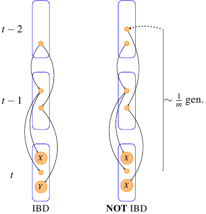
Our framework allows for a very natural definition of “kin” and “genetical identity by descent”, IBD for short (see Fig. 9). Say that two individuals in the same generation are -kin in case they share a common ancestor at most generations in their past. (The 1-kin of an individual are its siblings, its 2-kin are its siblings and cousins, etc.) Because the number of groups is large, individuals from different groups have negligible probability of being -kin, unless is comparable to . As for individuals in the same group, migration events in their lineages play a major role in their being or not kin. If, when we follow their lineages back in time, we find a migration event in one of these lineages before they coalesce, then we know that the probability that they will coalesce in a time that is much shorter than is negligible. With this in mind, say that two individuals in the same generation are IBD in case following their lineages backwards in time, they coalesce before (in the backwards sense) a migration event happens in either one. From the discussion above, we know that being IBD is essentially the same as being -kin for some that may have to be large, but is not comparable to .
We denote by the event that the focal and the co-focal individuals are IBD, and define genetic relatedness for the allele A by
In the E.S., is negligible, and so is also (we adopt the common convention of omitting the intersection symbol ). This implies that Using also (23), we have then
Combining this with (25), gives that
| (31) |
We look now into how the generalized Hamilton’s rule (26) can be written in the case in which is a linear function of . There is no loss in generality in supposing that this linear function can be written as , with constant. We could, for instance, be considering the public goods game, Example 1, or an additive pairwise interaction, Example 4. But note that we are not making any assumption about , so that all that we are assuming is that at a cost to itself, each altruist provides a benefit to each other altruist in its group. They may be providing benefits to non-altruists or not, and if they do, the amount of that benefit is irrelevant for the current computation. We do not need, in particular, to assume linearity of in . We are also not yet assuming any restrictions on the values of and .
The linearity of can be exploited by using (31) to write
This transforms (26) into the familiar expression of Hamilton’s rule:
| (32) |
whenever . But note that even in this case, in which and are constants, the relatedness complicates the application of the rule. To compute theoretically, one still needs information about . And if analyzing data from an experiment that is supposed to be well modeled by our framework, one would have to sample from the S.E.S., not from the very early stage (before stationarity settles in), or from the late stage when the number of altruists is no longer negligible as compared to the size of the whole population, so that the group type distribution is no longer directly related to . For field data, this remark may make (32) of little value. Fortunately, this problem disappears in the case of weak selection, as we will see later.
Condition (32) refers to the viability of a single new mutant A. It is clear that if we started from any number of copies of the gene A that were negligible as compared to , the same arguments would apply and lead to the same rule. But had we started in generation 0 from a distribution of groups with a non-negligible fraction of altruists, (32) would not in general provide us with the direction of evolution. Indeed, even the equilibria between alleles A and N, in the late stage of the evolution, will not in general turn the inequalities in (32) into equalities, unless . This point, that is emphasized in [70], is well illustrated by considering Example 4, in which . As is well known, for arbitrary and , we can write the Price equation (19), or (20) also in the following form, where :
where
and
(The second inequality in each one of these last two displays is analogous to (25), corresponding to averages over size biased samplings of the distribution .) In case , and , we can use (23) and (24), to reduce these to
Hence,
where is the synergy parameter, and we used (27) and (28). When , and , the necessary and sufficient condition for , is therefore
| (33) |
Condition (33) was derived in the case in [71], who called it Queller’s rule, giving credit to the work in [56]. We refer the reader to [63], for an extension of Queller’s rule when and are not linear functions of .
Consider now the threshold model in Example 3. In this case , so that the generalized Hamilton rule (26) reads
| (34) |
Comparing (32) with (34) is elucidating. Both make the heuristic power of (26) apparent: in both cases the cost incurred by carrying the gene A must be compensated by the expected benefit that it brings to its carriers. We will address in more detain in the next paragraph the fact that this expected value is in the particular distribution , related to . For the moment we focus on the fact that while (32) is in the usual Hamilton’s rule form, (34) is not. We do not see anything deep about this difference. The special form of (32), involving relatedness, is a feature of the linearity of , that allows one to break the computation of an expectation into a sum of correlations between the genotype of the focal and each one of its group companions, taken one at a time. In the case of (34), the threshold nature of , does not allow for such a decomposition in any meaningful and simple way, as far as we can see. Trying to rewrite in terms of the relatedness parameter in this case, does not seem a natural idea. But there isn’t anything really that fundamental about relatedness in (26). What is important there is the distribution of the random variable , i.e., the values of , . For a threshold model, the particular feature of this distribution that is of relevance is the tail probability . For a linear model the relevant aspect of this distribution is the expectation , that is naturally expressed in terms of relatedness, since , by (31). Trying to rewrite (34) in terms of relatedness seems as unnatural to us as trying to rewrite (32) in terms of the tail probabilities . In this connection, we refer the reader also to the conceptual discussion on this model, in the case , in [70] (where it was called “stag hunt game”), [44], [71] and [20]. Especially important is the fact that in [20] both, (33) and (34) are written in the traditional Hamilton form . This is accomplished there at the cost of defining and as appropriate regression coefficients, that depend not only on parameters in the payoff functions, but also on the distribution of genes A and N in the population (see, for instance, (12) and (13) in that paper). Conceptually, this raises the question of what and mean in Hamilton’s rule. Computationally, we have found it easier to compute directly with (33), (34) and more generally with the generalized Hamilton rule (11), or equivalently, (26), rather then with the methods from [20]. Their and vary in time, as the distribution of genes A and N changes. For instance, to rewrite our (34) in their Hamilton form , one has to consider the distributions of these genes in the S.E.S.. Therefore, one has to first find and then use it in the computations of and as regression coefficients. But once is obtained, (34) is available with little additional computational work, since . For this matter, obtaining directly, as Perron-Frobenius eigenvalue of , and using (11) is, off course, easier than using either (34), or the methods from [20]. This raises the question whether (34) is ever of computational value. The answer is positive, since in Section 5 we will see that (26) and, in particular, (34) yield simple and elegant formulas, when is small, and is large (see (61), (62) and the related Fig. 14).
The viability condition (26) and its special cases (32) and (34) are heuristically meaningful, but computationally and experimentally they may not be such an advance over (11). The distribution is built into , and in particular into and . Computationally, finding is at least as demanding as finding . Experimentally, one would not expect to sample in nature from the S.E.S., but rather from the late stage, after A has invaded and is now either fixated, or in a polymorphic equilibrium with N. (One can conceive, though, lab experiments in which one could sample from the S.E.S..) Fortunately, these problems disappear when selection is weak, as we will see next.
4 Weak selection and further conceptual discussion
We turn now to simplifications to our analysis in case of small , i.e., weak selection. In this case it is well known (see, e.g., [59], [40]) that there is a separation of time scales. Most of the time in most places evolution is occurring as if were 0, i.e., via neutral genetic drift. Only occasionally events happen that are caused by the slight differences in fitness of the individuals. Mathematically, what one gains is the possibility of studying the process as a perturbation of the neutral evolution. For us, this will be encapsulated in a result that we state next. We will include now as a superscript in the notation of quantities that depend on it (e.g., , , , , , etc).
We observe that when is small enough, the generalized Hamilton rule (11) and its equivalent (26) can be replaced by the requirement that
| (35) |
Indeed, (35) is an immediate consequence of (26), due to the continuity of the Perron-Frobenius left-eigenvector of the matrix as a function of . As , the vector converges to , the Perron-Frobenius left-eigenvector of the matrix . Importantly, , and hence also , does not depend at all on the payoff functions. They depends only on and . This is illustrated in Fig. 8, where one can see that is model dependent for large , but becomes model independent under weak selection.
The important simplification in (35), with respect to (26), is that has been replaced by in the left hand side of (26). In particular, (35) is not affected by the values of . This may seem surprising at first sight, but can be understood as follows. In the E.S., most type N individuals are in groups without altruists, so that the mean fitness of the gene N is close to 1, not depending on the . The values of the do affect the distribution , because they affect the fate of the groups with altruists, and in this way affect the mean fitness of the gene A. (This is how the affect (26) and its special cases (32) and (34).) But when is small, is close to , and its dependence on and is a perturbation of order . This dependence produces only a second order effect (of order ) on .
Conceptually, one can see (35) as a separation of the effects from demographics from those of fitness. The distribution is completely determined by the demographics, while the payoffs carry only information about the fitness function. This separation makes the concept of neighbor modulated fitness particularly appealing in the regime of weak selection. The viability condition (35) says that the mutant gene A is viable in case its average (neighbor modulated) fitness is larger than that of the wild type N before A appeared, with the weights in the average being given by the fashion in which the demographics alone arranges the genes in the population.
For theoretical analysis, (35) is much simpler than (11), or (26). One can compute once and for all the distributions , that depend only on and . Then, in analyzing a model (given by and ), one simply looks at the average value of with respect to the universal distribution . This allows for a much greater intuition of what to expect, when comparing models, than was possible in the case of strong selection, in which and also affect the distribution . For instance, if two models I and II are comparable in the sense that , , then we have . This allows one to use a simple model, like the threshold model in Example 3, to obtain estimates (say, lower bounds) on the value of for more interesting and realistic models, like those in Examples 2, 5 and 6.
The viability condition (35) still refers to the S.E.S., but this can be overcome by considering a different random variable instead of . Define as the number of individuals in the group to which the focal belongs, that are IBD to the focal (the focal included in the counting). Clearly , and, with overwhelming probability, in the E.S.. Observe that , for all , since conditioning on does not affect lineages, when . But while depends on the fraction of altruists in the population, and so changes with time, becomes constant for (or, more precisely, for , so that by time it is likely that migration events have occurred in the focal’s lineage). We denote by this equilibrium distribution:
Considering in the S.E.S., which has both , and , gives then
| (36) |
And the viability condition (35) can be rewritten as
| (37) |
This is a major improvement over (11) and (26), since now no reference to the S.E.S. is left. The distribution only depends on the structure of the population and how genes flow under neutral drift. Experimentally it can be accessed by sampling any neutral genetic markers from the population in demographic equilibrium (the condition ).
The distribution is directly associated to the relatedness , , in the same way that the distribution is associated to . Recall the enumeration of the members of the focal group, in which the first individual is the focal. Now decompose , where, , if the th individual in this ordering is IBD to the focal, and , otherwise. This yields , and therefore
| (38) |
for , where the last equality introduces a new notation.
One can compute relatively easily, as follows. If either the focal or the co-focal are migrants, they are not IBD. If they are both non-migrants, they chose their parents from the parental group of their group. With probability they chose the same parent, and are therefore IBD. With probability they chose different parents. In this last case they are IBD exactly if their parents are IBD, and this event has probability . Assembling these pieces, we obtain and hence,
| (39) |
where the approximation is good when is small. This a well known result by Wright for the infinite islands model, for haploid individuals. It is important to clarify that even when , our framework is not identical to the infinite islands model. In that model there are a large number (to be taken to in the computations) of islands, each one with individuals. In generation the individuals in each island choose, independently, a parent from the individuals in the same island in generation . This is followed by migration at rate , that is implemented in exactly the same way as in our framework. Differently from our framework, each island is “parent” to exactly one island in the next generation. In our framework, when , each group is parent to a random number, with distribution , of groups. In spite of this difference, it is not simply a coincidence that lead to the same formula (39) in both frameworks. They share the same coalescence structure, when we ask ourselves questions related to IBD. Not only is identical in these frameworks, but so is also the distribution . Indeed, when we follow lineages backwards in time, until there are migration events, it does not matter if the group that we are following from generation to generation is the same (as in the infinite islands case) or changes (as in our case).
We will show next that
| (40) |
when , so that can also be obtained experimentally from standard statistical regression methods (for instance using (30)), applied to neutral genetic markers, by sampling from a single generation , without information about past generations or any knowledge about kinship.
To emphasize where in the proof of (40) the assumption will matter, we first write, for arbitrary ,
Clearly , . The fact that allows the following simplifications:
so that also
and
(This would generally not hold with , since then information on the occurrence or not of biases the lineage of the co-focal, even if it does not meet that of the focal.) With the simplifications above, we readily obtain (40).
The identity (39) shows that, as expected, is a strictly decreasing function of . This identity can be inverted as
| (41) |
With fixed there is a 1-to-1 correspondence between and , given by (39) and (41). It is natural then, in the regime of weak selection, to define the critical value of as
| (42) |
This is the least level of relatedness that makes the gene A viable in our framework, under weak selection. Even when selection is not weak, we can define via (42), since is a natural alternative way to identify the value of , through (39), and can be measured using neutral genetic markers. See Fig. 13 for the shape, on a logarithmic scale of the function (42).
Under weak selection, when is a linear function of , as in the public goods game, or additive pairwise interactions, the viability condition (32) now reads
| (43) |
This is a fully standard Hamilton rule, with independent of and , being a function only of the population structure, through and . The critical values are therefore
| (44) |
where we used (41), and the approximate result is valid when is large.
Condition (43) is an expression in our setting of the common wisdom according to which Hamilton’s rule in its standard form applies when selection is weak and interactions are pairwise and additive (Example 4, in our setting). In this regard, there are several points worth commenting.
First, (43) holds with no assumption on , so that it goes beyond that common wisdom.
Second, that as explained after (32), we are only considering a viability condition for an initial situation with a single (or for this matter, a number ) of type A individuals. Even in the case of weak selection, and with pairwise additive interactions (so that , ), when the numbers of type A and type N are comparable to , the condition for selection to increase the frequency of type A is given by Queller’s rule (33), that now reads
| (45) |
where, as before, and is the fraction of type A in the population.
Third, the assumption of weak selection greatly simplifies relatedness, and makes it more universal, but otherwise, also under strong selection (32) has the usual Hamilton rule form.
Fourth, in our setting it is not the pairwise additive nature of the interaction that matters. What matters for (32) and (43) to hold is linearity of in (and for (33) and (45) to also hold, additional linearity of in ), so that one can use (23) and (24). In Example 4, we explained that this sort of linearity is formally equivalent to having pairwise additive interactions, but it can also result from interactions involving many individuals at the same time, as in Example 1.
Fifth, the meaning of and in (43) has to be carefully understood. This point is well illustrated by considering the fitnesses in (18), that corresponds to the case of pairwise interactions in iterated prisoners dilemmas, with types N always defecting and types A playing tit-for-tat. In this case and , where is the cost to an actor each time it cooperates, is the benefit that an actor provides to its partner each time it cooperates, and is the average number of iterations of each pairwise interaction. The viability condition (43) now reads and we have
| (46) |
For we have , but decreases as increases. Nothing here is surprising, but these computations illustrate the fact that and are life-cycle costs and benefits, and not costs and benefits in each momentary interaction (even if those are constant, as in the present case).
In contrast to (43), the weak selection form of the viability condition (34), for the threshold model, Example 3, reads
| (47) |
The quantity depends only on and . Thanks to (41), it can also be seen as a function of and only. But we see no hope in expressing this functional dependence in simple terms, that would allow us to derive a simple expression for in this example. We will, nevertheless, obtain interesting approximations for it in Section 5. We will also be able there to compute the exact limit of for this example, as , provided that for some constant .
To apply the viability condition (37), we need to compute . One solution is to find , and use (36). And can be computed as the Perron-Frobenius left-eigenvector of , where
This yields, after some simplifications,
| (48) |
Moreover, one can use the fact that to further simplify the computation of .
One can also use, alternatively, methods from coalescence theory, to study the distribution . But because we find these methods quite cumbersome for this purpose, we introduce next a further alternative approach, illustrated in Fig. 10, and explained next.
Consider again the random experiment of choosing a focal individual from generation . Denote by , , the ancestor of the focal in generation , so that, in particular, is the focal. Denote by the group to which belonged. Then denote by the number of members of that where IBD to the focal’s ancestor (including itself). Our basic observation is that, when , so that there is no selection, the sequence of random variables forms a time-stationary Markov chain on the set , described as follows. Given the value of , the value of is:
-
(MC1) With probability , set to 1. [Migration event in focal’s line of descent.]
-
(MC2) With probability set equal to . [No migration event in focal’s line of descent.]
This corresponds to a transition matrix (that does also not depend on ) given by:
| (49) |
To understand this claim, first observe that if the ancestor of the focal in generation , was a migrant, then, by definition of IBD, we have in no one other than itself IBD to , and hence . This corresponds to (MC1) above. On the other hand, if was not a migrant, then the number, of other members of that were IBD to is easily obtained as follows. Each one of the other members of chose independently a parent from . The group had members that were IBD to (with included). Members of other than became IBD to if two conditions were satisfied: they had to choose a member of that was IBD to , and they had to stay in the group , rather than migrate out. (If they migrated out, their replacements would not be IBD to , by definition of IBD). Each one of these individuals in had, therefore, independently, probability of being IBD to . This gives for the binomial probability in (MC2). Adding 1, for itself, gives us the full expression in (MC2).
The Markov chain , starts from , and when it will have reached its stationary state . (It is clear that the chain is irreducible and aperiodic when , since in this case all entries of are strictly positive. In case , it is clear that the chain converges to its single absorbing state , so that . In case , it is clear that the chain converges to its single absorbing state , so that .) One can compute using stationarity, by solving the linear system of equations
| (50) |
Identity (36), relating and , can now be alternatively derived by observing that, from (48) and (49), we have .
The distribution enjoys a nice monotonicity property, as a function of . We recall that a probability distribution over is said to be stochastically larger than another one, , if , for . In this case we write . It is known that this relationship is equivalent to the statement that , whenever is increasing in . We claim that is stochastically monotone decreasing in , i.e.,
| (51) |
Therefore, under (C4), the left hand side of (37) is decreasing in . In particular, there can only be one value of that satisfies . The claim (51) follows from the double observation that is stochastically decreasing in and stochastically increasing in . (To see this more easily, consider the description of in (MC1) and (MC2) above. Note that with fixed, increasing decreases , and that with fixed, is increasing with .) We can use the monotonicity in in this observation, to write, whenever ,
Now, we can use the monotonicity in in the observation above to iterate this inequality and obtain , for arbitrary . Letting , gives .
The Markov chain introduced above can also be used in other ways, by allowing one to write recursions for quantities of interest. For instance, this method can be used for computing the moments of the distribution , , . This is in principle very useful, since an arbitrary can always be approximated by a polynomial. So, in theory, one can compute in good approximation and, through (37) compute also in good approximation. We will see in the next section, that in spite of the expressions for the moments being quite involved, they provide very powerful information. The heuristic nature of the recursive method requires going behind the apparently cryptic expression for , and instead using its description in items (MC1), (MC2), that appears immediately before was introduced. We illustrate the method computing first the mean of , . When the Markov chain is stationary, both and have distribution . Therefore, from (MC1) and (MC2) we obtain:
This yields
| (52) |
This result could also have been obtained by combining (38) and (39), or alternatively (39) could have been obtained from (38) and (52).
To express the th moment, , in terms of , , we will use the following fact. If has a distribution, then
where , and the Stirling number of the second kind, , is the number of ways in which a set with elements can be partitioned into non-empty sets. Clearly , for all . They are also known to satisfy
The first few values of are:
For our purpose, it is convenient to write , and use the Markov chain description (MC1), (MC2) as it applies to : With probability this quantity takes the value 0, and with probability it takes the value . Therefore
Since in equilibrium, and both have distribution , we obtain
This provides us with the aimed recursion:
| (53) |
This gives for the variance of the distribution the value:
The expressions above for and the variance are obviously very involved. They simplify substantially when is large, since as . This is not a surprise, since does not appear in (MC1), and in (MC2) the binomial random variable converges in distribution to a Poisson random variable, with mean . The resulting Markov chain has state space , but it is not hard to show that it is positive recurrent, and so has a single stationary distribution, to which converges as . We will not explore this limit here, but rather study, in the next section, a limit in which as , also . As we will see, in this limit simplifies considerably, and leads to a number of very interesting applications.
5 Limit of large n and small m under weak selection
In this section we will continue to assume that selection is weak and we will study the limit in which
| (54) |
where we used (39). To state the results on the behavior of the distribution in this limit, we suppose that is a random variable with distribution , i.e., . We state and comment the results in (a) and (b) below, and afterwards, explain how to do the computations. (See also Fig. 12.)
(a) If , then for ,
| (55) |
This implies (see, e.g., Section 2.3.e of [11]) that the random variable converges in distribution to a distribution with th moment .
When , these moments characterize a Beta distribution, with parameters and , which has density , . In other words,
| (56) |
for arbitrary . Notice that, for each , this tail probability, , is decreasing in , meaning that the corresponding family of Beta distributions is stochastically monotone decreasing in .
The case , which has , is particularly simple. In this case the limiting distribution, Beta(1,1) is the uniform distribution between 0 and 1, with , . This case can be seen as separating two qualitatively distinct cases: When , the density is increasing in , while when , the density is decreasing in . In the extreme cases, in which is close to 0 or very large, the density concentrates, respectively, close to 1 or 0.
When , we have , for each . These are the moments of a degenerate random variable, that takes the value 1 with probability 1. Therefore the random variable converges in probability to 1.
(b) If , we have for ,
| (57) |
These are the moments of a degenerate random variable, that takes the value 0 with probability 1. Therefore the random variable converges in probability to 0.
But a different way of scaling , provides a non-degenerate limit. We have, for ,
| (58) |
i.e., converges in distribution to a random variable with th moment . These moments characterize an exponential distribution with mean . In other words,
| (59) |
for arbitrary .
The claims in (55), (57) and (58), about the convergence of the scaled moments, can be readily obtained by induction in , from (52) and (53), and the following two observations. First, for ,
Second, the denominator in (53) can be rewritten as
where and .
A question that comes naturally to mind is whether for the threshold model in Example 3, we can find the exact value of , in the case of weak selection. Unfortunately we have not been able so far to compute the exact value of . We can, nevertheless, use the result in (56) above, that states that when is large and is small, then . Using this approximation in combination with (47), yields
| (61) |
This approximation should be good when is large, and is not too close to 0, so that the resulting value of is small. When, additionally, is substantially smaller than 1, we can further approximate
| (62) |
See Fig. 14, for a comparison of the exact value of under weak selection, from the viability condition (37) (or, equivalently, (47)) and the approximations (61) and (62). Surprisingly, (61) gives a good approximation there even when is small.
The approximation (61) for Example 3 can be formalized and extended to a wide class of models in the following way. (See Fig. 16, for an illustration.) Suppose that there is a piecewise continuous and bounded function , , such that
| (63) |
Then, the result in (56) above, combined with the continuous mapping theorem, (2.3) in Section 2.2.b of [11], implies that, when ,
| (64) |
in the limit (54), where the last equality introduces a new notation. This means that, in this limit, the viability condition (37) now reads
| (65) |
We want to define as the solution of
| (66) |
To assure that this equation has a solution it is sufficient to assume that is continuous at the end-points and . In this case, under under (C1),
as . And under (C2),
as . Since clearly is continuous in , (66) then must have a solution . If there is more than one solution, then we define as the largest one. If condition (C4) holds, then is non-decreasing in . In this case, the stochastic monotonicity of the Beta distributions in (a) imply that is non-increasing in . Actually, it is clear, from the behavior of the density , that is then strictly increasing in , unless is constant. Hence, when is continuous at 0 and 1 and (C1), (C2) and (C4) hold, (66) defines uniquely.
The viability condition (65) implies that if we consider a model that satisfies (63), then in the weak selection regime,
| (67) |
Example 3 satisfies (63), if we take , for some , where is the smallest integer larger than or equal to . In this case, , for , and , for . This yields , and therefore
The approximation (61) can be seen now as a special case of (67).
Example 2 also satisfies (63), if we take , for some , where is the largest integer smaller than or equal to (the integer part of ). In this case, , for , and , for . (See Fig. 16.) Condition (14) is satisfied, when is large, in case , and fails if . In case , (14) may be satisfied or fail, depending on whether is close to or , but in either case, the left hand side of (14) is of order , so that it is only marginally satisfied or violated. In our analysis below, we will not assume that (14) holds. We have, for this model,
Equation (66), does not lead in this case to a simple expression for , as it did in Example 3. We can nevertheless still derive very useful information from it. To simplify the resulting equation, set . Then (66) reads
| (68) |
except in the trivial case , in which the right hand side of (68) is 0. This case corresponds to , so that types A cooperate only in the first round. Obviously then, Example 2 reduces to Example 1, and indeed, (68) reduces to (43).
In the opposite extreme, when , so that and types A cooperate in each round of the game, the right hand side of (68) reduces to . So (68) is again reduced to (43), as one should expect.
Note that also when , Example 2 reduces to Example 1, and (68) reduces to Hamilton’s rule (43). One can see the right hand sight of (68), as a correction to that form of the viability condition in the more general Example 2.
Fig. 15 compares the exact values of and for instances of Example 2, under weak selection, from the viability condition (37), and the approximation provided by solving (68). Notice in these graphs, that is significantly smaller than , when is close to .
While somewhat intimidating at first sight, (68) provides good information about the critical value . We first state the main features of its behavior, and then explain how to do the computations leading to these claims. Of special importance is the case in which . In this case (68) simplifies to:
| (69) |
With , and fixed, is a continuous function of , that takes the value on both end-points of this domain, is strictly decreasing when , and strictly increasing on . It reaches therefore its minimum at , where it solves (69). It is not surprising that when , so that (14) is satisfied, we have , since in this case, when altruists continue cooperating, it is always in their interest to do so. But it is somewhat surprising that also when , we have . It is intuitive that should reach its minimal value when , since then altruists are persisting precisely when they should.
With and fixed, is a decreasing function of , that goes to 0 as (Fig. 17). With , and fixed, is a decreasing function of that behaves as follows when . If , then , while if , then . In this latter case, the convergence is rather slow, in that behaves asymptotically as . (See Fig. 18.)
The claims above follow from the behavior of the left hand side and the right hand side of (68). We denote them respectively by and . (With , so that is continuous on the interval . Note that not only , but also all its derivatives converge to 0 as .) See Fig. 19, for an illustration of what follows. The function is very straightforward; it is a strictly decreasing function of , that is positive for and negative for . The function has the sign of the term inside the curly braces. That term inside the curly braces is 0 when . We define , and observe that , when , and , when . The term inside the curly braces, and therefore also , is negative for , and positive for . Notice also that once it is positive, is strictly increasing in , since it is then the product of strictly increasing positive functions. The behaviors described so far for and immediately imply that they are equal to each other at exactly one point , and that this point is in the open interval .
The various claims about the behavior of as a function of , or of , or of , follow now from analyzing the behavior of the graphs of and of , as these parameters change. We have , which, regardless of the value of , is positive for and negative for . This means that the graph of moves upwards, as increases from 0 to , and then moves downwards, as increases from to 1. In the extremes, , as , for all . (This convergence is not uniform, since the function converges to 0 as .) And , uniformly in , as . These facts, and the trivial behavior of that does not depend on , provides us with the facts about the dependence of on .
The fact that depends on and only through can be seen by dividing both sides of (68) by . The fact that decreases as increases follows easily from observing that the graphs of and move, respectively, down and up, as increases, with fixed. And the fact that , as , is immediate from (Fig. 17).
If we keep , and fixed and let , then also goes monotonically to , for , and stays at 0 for . The corresponding behavior of the graph of , and the fact that is the point in where this graph intersects the graph of the decreasing function , shows that, as claimed above, is decreasing in , and as , (Fig. 20). The claim about the slow speed of this convergence, in case , can be obtained by taking the logarithm of both sides of (68) and analyzing how the resulting terms behave as .
It is interesting to contrast (46), for iterated pairwise prisoner dilemma with types N defecting and types A playing tit-for-tat (Example 4, (18)) with our analysis above of the behavior of in Example 2, which is an iterated public goods game (an analogue of the prisoner dilemma in a multi-individual setting), with types N defecting and types A playing many-individual tit-for-tat. There are several expected similarities in the behavior of in both cases, as a function of costs, benefits and expected number of repetitions of the game. But there are also important differences to emphasize. There are differences in the details of the behavior. For instance, goes to 0, as , much more slowly in the case of Example 2, when it does go to 0. But equally important, we want to mention the differences in the level of complexity of the analysis in each case. While (46) holds for arbitrary and resulted from a standard Hamilton rule, (43), our analysis of Example 2 above relied on the much more elaborate results developed in this section, and depended on being large. One of the main messages of the current paper is that when interactions involve several individuals at a time in the groups, one needs methods that go beyond those that apply to pairwise additive interactions.
It is important to explain why the assumptions made in [7] on how much assortment to expect in Example 2, and later used in several papers, including [6], are excessively pessimistic. In [7] it was supposed that conditioned on the focal individual being type A, the other members of the focal group would be type A independently, with probability . In our framework, given that the focal is type A, and that the co-focal is also type A, further increases the conditional probability that a third member of the group is type A. Given then that a third individual is type A, again further increases the probability that a fourth individual is type A, and so on. This is so because the information being successively provided keeps increasing the probability that there were several types A in the previous generation in the group from which the focal descends. It is very interesting to make the computation of using the assumption of [7] and compare the result with what we have obtained from (68). Under that assumption of conditional independence, the viability condition (37) for the regime of weak selection, would be replaced with . Assume that (63) holds and define as , when is a continuity point of , and as the average between the limits of from the left and from the right at , otherwise. (We are supposing that these limits exist, as is the case in Example 2.) Then, by a central limit theorem, in the limit (54).
(Compare with (64).) Instead of (66), we would then have
| (70) |
For Example 2, the only solution of (70) is , regardless of the value of . This result would not depend on , and would differ substantially from our result in case, e.g., , large, which has . (See Fig. 15, Fig. 17, Fig. 18 and Fig. 20.)
References
- [1] Abbott, P., et. al. (2011) Inclussive fitness theory and eusociality. Nature 471, E1-E4.
- [2] Aoki, K. (1982) A condition for group selection to prevail over counteracting individual selection. Evolution 36, 832-842.
- [3] Axelrod, R. (1984) The Evolution of Cooperation (Basic Books).
- [4] Boomsma, J.J., Beekman, M., Cornwallis, C.K., Griffin, A.S., Holman, L., Hughes, W.O.H., Keller, L., Oldroyd, B.P. and Ratnieks, F.L.W. (2011) Only full-sibling families evolved eusociality. Nature 471, E4-E5.
- [5] Bowles, S., Gintis, H. (2011) A Cooperative Species: Human Reciprocity and its Evolution. (Princeton University Press, Princeton).
- [6] Boyd, R., Gintis, H., Bowles, S. (2010) Coordinated punishment of defectors sustains cooperation and can proliferate when rare. Science 328, 617-620.
- [7] Boyd, R. and Richerson, P.J. (1988) The evolution of reciprocity in sizable groups. Journal of Theoretical Biology 132, 337-357.
- [8] Chuang, J.S., Rivoire, O. and Leibler, S. (2010) Cooperation and Hamilton’s rule in a simple microbial system. Molecular Systems Biology 6, 398-344.
- [9] Cohen, D. and Eshel, I. (1976) On the founder effect and the evolution of altruistic traits. Theoretical Population Biology 10, 276-302.
- [10] Crow, J.F. and Aoki, K. (1982) Group selection for a polygenic behavioral trait: a differential proliferation model. Proceedings of the National Academy of Sciences of the United States of America 79, 2628-2631.
- [11] Durrett, R. (2005) Probability: Theory and Examples (Thomson, Brooks/Cole, London).
- [12] Eshel, I. (1972) On the neighbor effect and the evolution of altruistic traits. Theoretical Population Biology 3, 258-277.
- [13] Fehr, E. and Fischbacher, U. (2003) The nature of human altruism. Nature 425, 785-791.
- [14] Ferriere, R. and Michod, R.E. (2011) Inclusive fitness in evolution. Nature 471, E6-E8.
- [15] Fletcher, J.A. and Doebeli, M. (2009) A simple and general explanation for the evolution of altruism. Proceedings of the Royal Society B 276, 13-19.
- [16] Fletcher, J.A., Zwick, M., Doebeli, M. and Wilson, D.S. (2006) What is wrong with inclusive fitness? Trends in Ecology and Evolution 21, 597-598.
- [17] Foster, K.R., Wenseleers, T. and Ratnieks, F.L.W. (2006) Kin selection is the key to altruism. Trends in Ecology and Evolution 21, 57-60.
- [18] Foster, K.R., Wenseleers, T., Ratnieks, F.L.W. and Queller, D.C. (2006) There is nothing wrong with inclusive fitness. Trends in Ecology and Evolution 21, 599-600.
- [19] Frank, S.A. (1998) Foundations of Social Evolution (Princeton University Press, Princeton).
- [20] Gardner, A., West, S.A. and Wild, G. (2011) The genetical theory of kin selection. Journal of Evolutionary Biology 24, 1020-1043.
- [21] Goodnight, C.J. (2005) Multilevel selection: the evolution of cooperation in non-kin groups. Population ecology 47, 3-12.
- [22] Goodnight, C.J. and Stevens, L. (1997) Experimental studies of group selection: what can they tell us about group selection in nature? The American Naturalist 150, S59-S79.
- [23] Grafen, A. (2006) Optimization of inclusive fitness. Journal of Theoretical Biology 238, 541-563.
- [24] Grafen, A. (2007) Detecting kin selection at work using inclusive fitness. Proceedings of the Royal Society B 274, 713-719.
- [25] Haldane, J.B.S. (1932) The Causes of Evolution. (Longmans Green, London).
- [26] Hamilton, W.D. (1996) Narrow Roads of Gene land. (W.H. Freeman, Oxford).
- [27] Harpending, H. and Rogers, A. (1897) On Wright’s mechanism for intergroup selection. Journal of Theoretical Biology 127, 51-61.
- [28] Harris, T.E. (1989) The Theory of Branching Processes (Dover Publications, New York).
- [29] Hauert, C., Michor, F., Nowak, M.A. and Doebeli, M. (2006) Synergy and discounting of cooperation in social dilemmas. Journal of Theoretical Biology 239, 195-202.
- [30] Henrich, J. (2004) Cultural group selection, coevolutionary processes and large scale cooperation. Journal of Economic Behavior & organization 53, 3-35.
- [31] Herre, E.A. and Wcislo, W.T. (2011) In defence of inclusive fitness theory. Nature 471, E8-E9.
- [32] Joshi, N.V. (1987) Evolution of cooperation by reciprocation within structured demes. Journal of Genetics 66, 69-84.
- [33] Keller, L., ed. (1999) Levels of Selection in Evolution (Princeton University Press, Princeton).
- [34] Kelley, J.K. 1992 Restricted migration and the evolution of altruism. Evolution 46, 1492-1495.
- [35] Kerr, B. (2009) Theoretical and experimental approaches to the evolution of altruism and the levels of selection. In: Experimental Evolution: From Selection Experiments. Garland, T. and Rose, M.R., eds. (University of California Press, Berkeley, CA) 585-630.
- [36] Kerr, B. and Godfrey-Smith, P. (2002) Individual and multi-level perspective on selection in structured populations. Biology and Philosophy 17, 477-517.
- [37] Kerr, B., Godfrey-Smith, P. and Feldman, M.W. (2004) What is altruism? Trends in Ecology and Evolution 19, 135-140.
- [38] Killingback, T., Bieri, J. and Flatt, T. (2006) Evolution in group-structured populations can resolve the tragedy of the commons. Proceedings of the Royal Society B 273 1477-1481.
- [39] Lehmann, L. and Keller, L. (2006) The evolution of cooperation and altruism - a general framework and a classification of models. Journal of Evolutionary Biology 19 1365-1378.
- [40] Lehmann, L., Keller, L., West, S. and Roze, D. (2007) Group selection and kin selection: Two concepts but one process. Proceedings of the National Academy of Sciences of the United States of America 104 6736-6739.
- [41] Lehmann, L. and Rousset, F. (2010) How life history and demography promote or inhibit the evolution of helping behaviors. Philosophical Transactions of the Royal Society B 365, 2599-2617.
- [42] Maynard Smith, J. (1964) Group selection and kin selection. Nature 201, 1145-1147.
- [43] Maynard Smith, J. (1976) Group selection. The Quarterly Review of Biology 51, 277-283.
- [44] Marshall, J.A.R. (2011) Queller’s rule OK: Comment on van Veelen ‘When inclusive fitness is right and when it can be wrong’. Journal of Theoretical Biology 270, 185 - 188.
- [45] Matessi, C. and Jayakar, S.D. (1976) Conditions for the evolution of altruism under Darwinian selection. Theoretic Population Biology 9, 360-387.
- [46] Matessi, C. and Karlin, S. (1984) On the evolution of altruism by kin selection. Proceedings of the National Academy of Sciences of the United States of America 81, 1754-1758.
- [47] McElreath, R. and Boyd, R. (2007) Mathematical Models of Social Evolution (The University of Chicago Press, Chicago and London).
- [48] Nowak, M.A. (2006) Evolutionary Dynamics: Exploring the Equations of Life. (Harvard University Press. Cambridge, MA).
- [49] Nowak, M.A. (2006) Five rules for the evolution of cooperation. Science 314 1560-1563.
- [50] Nowak, M.A., Tarnita, C.E. and Wilson, E.O. (2010) The evolution of eusociality. Nature 466, 1057-1062.
- [51] Nowak, M.A., Tarnita, C.E. and Wilson, E.O. (2011) Reply to [1], [4], [65], [14] and [31]. Nature 471, E9-E10.
- [52] Nunney, L. (1985) Group selection, altruism, and structured-deme models. The American Naturalist 126, 212-230.
- [53] Okasha, S. (2006) Evolution and the levels of selection (Oxford University Press, Oxford).
- [54] Okasha, S. (2010) Altruism researchers must cooperate [Comment]. Nature 467, 653-655.
- [55] Pepper, J.W. (2001) Relatedness in trait group models of social evolution. Journal of Theoretical Biology 206, 355-368.
- [56] Queller, D.C. (1985) Kinship, reciprocity and synergism in the evolution of social behavior. Nature 318 366-367.
- [57] Queller, D.C. (1992) Quantitative genetics, inclusive fitness, and group selection. The American Naturalist 139 540-558.
- [58] Rogers, A.R. (1990) Group selection by selective emigration: the effects of migration and kin structure. The American Naturalist 135, 398-413.
- [59] Rousset, F. (2004) Genetic Structure and Selection in subdivided populations. (Princeton University Press. Princeton).
- [60] Schonmann, R.H., Vicente, R. and Caticha, N. (2011) Generalized two-level Fisher-Wright framework with selection, migration and mutation. In preparation.
- [61] Schonmann, R.H., Vicente, R. and Caticha, N. (2011) Altruistic punishment can proliferate under extremely low levels of relatedness. In preparation.
- [62] Sigmund, K. (2010) The Calculus of Selfishness. (Princeton University Press, Princeton).
- [63] Smith, J., Van Dyken, D. and Zee, P.C. (2010) A generalization of Hamilton’s rule for the evolution of microbial cooperation. Science 328, 1700-1703.
- [64] Sober, E. and Wilson, D.S. (1998) Unto Others: The Evolution and Psychology of Unselfish Behavior. (Harvard University Press, Cambridge, MA).
- [65] Strassmann, J.E., Page Jr., R.E., Robinson, G.E. and Seeley, T.D. (2011) Kin selection and eusociality. Nature 471, E4-E5.
- [66] Traulsen, A. (2009) Mathematics of kin- and group-selection: Formally equivalent? Evolution 64, 316-323.
- [67] Traulsen, A. and Nowak, M.A. (2006) Evolution of cooperation by multilevel selection. Proceedings of the National Academy of Sciences of the United States of America 103, 10952-10955.
- [68] Trivers, R.L. (1971) The evolution of reciprocal altruism. T͡he Quarterly Journal of Biology 46, 35-47.
- [69] Uyenoyama, M. and Feldman, M.W. (1980) Theories of kin and group selection: some theoretical ambiguities. Theoretical Population Biology 17, 380-414.
- [70] van Veelen, M. (2009) Group selection, kin selection, altruism and cooperation: when inclusive fitness is right and when it can be wrong. Journal of Theoretical Biology 259, 589-600.
- [71] van Veelen, M. (2011) A rule is not a rule if it changes from case to case (a reply to Marchall’s comment). Journal of Theoretical Biology 270, 189-195.
- [72] Wade, M.J. (1985) Soft selection, hard selection, kin selection, and group selection. The American Naturalist 125, 61-73.
- [73] Wade, M.J., Wilson, D.S., Goodnight, C., Taylor, D., Bar-Yam, Y., de Aguiar, M.A.M., Stacey, B., Werfel, J., Hoelzer, G.A., Brodie III, E.D., Fields, P., Breden, F., Linksvayer, T.A., Fletcher, J.A., Richerson, P.J., Bever, J.D., Van Dyken, J.D. and Zee, P. (2010) Multilevel and kin selection in a connected world. Nature 463, E8-E9.
- [74] Wenseleers, T. (2006) Modeling social evolution: the relative merits and limitations of a Hamilton’s rule-based approach. Journal of Evolutionary Biology 19, 1419-1422.
- [75] Wenseleers, T., Gardner, A. and Foster, K.R. (2010) Social evolution theory: a review of methods and approaches. In: Social Behaviour: Genes, Ecology and Evolution. Szekely, T., Moore, A.J. and Komdeur, J., eds. (Cambridge University Press) 132-158.
- [76] West, S.A., El Mouden, C. and Gardner, A. (2010) Sixteen common misconceptions about the evolution of cooperation in humans. Evolution and Human Behavior (in press).
- [77] West, S.A., Griffin, A.S. and Gardner, A. (2007) Evolutionary explanations for cooperation. Current Biology 17, R661-R672.
- [78] West, S.A., Griffin, A.S. and Gardner, A. (2007) Social semantics: altruism, cooperation, mutualism, strong reciprocity and group selection. Journal of Evolutionary Biology 20, 415-432.
- [79] West, S.A., Griffin, A.S. and Gardner, A. (2007) Social semantics: how useful has group selection been. Journal of Evolutionary Biology 21, 374-385.
- [80] Wild, G., Gardner, A. and West, S.A. (2009) Adaptation and the evolution of parasite virulence in a connected world. Nature 459, 983-986.
- [81] Wild, G., Gardner, A. and West, S.A. (2010) Replying to Wade, et. al. [73] Nature 463, E9-E10.
- [82] Wilson, D.S. (1980) The Natural Selection of Populations and Communities (Benjamin/Cummings, Menlo-Park, CA).
- [83] Wilson, D.S. (1990) Weak altruism, strong group selection. Oikos 59, 135-140.
- [84] Wilson, D.S. (2007) Social semantics: toward a genuine pluralism in the study of social behavior. Journal of Evolutionary Biology 21, 368-373.
- [85] Wilson, D.S. and Wilson, E.O. (2007) Rethinking the theoretical foundation of sociobiology The Quarterly Review of Biology 82, 327-348.
- [86] Wilson, E.O. and Hölldobler, B. (2005) Eusociality: Origins and consequences. Proceedings of the National Academy of Sciences of the United States of America 102 13367-13371.
- [87] Wright, S. (1945) Review: tempo and mode in evolution: a critical review. Ecology 26, 415-419.