Symmetry protected topological (SPT) phases are gapped short-range-entangled quantum phases with a symmetry $G$. They can all be smoothly connected to the same trivial product state if we break the symmetry. The Haldane phase of spin-1 chain is the first example of SPT phases which is protected by $SO(3)$ spin rotation symmetry. The topological insulator is another example of SPT phases which is protected by $U(1)$ and time reversal symmetries. In this paper, we show that interacting bosonic SPT phases can be systematically described by group cohomology theory: distinct $d$-dimensional bosonic SPT phases with on-site symmetry $G$ (which may contain anti-unitary time reversal symmetry) can be labeled by the elements in ${\cal H}^{1+d}[G,U_{T}(1)]$ – the Borel $(1+d)$-group-cohomology classes of $G$ over the $G$-module $U_{T}(1)$. Our theory, which leads to explicit ground state wave functions and commuting projector Hamiltonians, is based on a new type of topological term that generalizes the topological $\theta$-term in continuous non-linear $\sigma$-models to lattice non-linear $\sigma$-models. The boundary excitations of the non-trivial SPT phases are described by lattice non-linear $\sigma$-models with a non-local Lagrangian term that generalizes the Wess-Zumino-Witten term for continuous non-linear $\sigma$-models. As a result, the symmetry $G$ must be realized as a non-on-site symmetry for the low energy boundary excitations, and those boundary states must be gapless or degenerate. As an application of our result, we can use ${\cal H}^{1+d}[U(1)\rtimes Z_{2}^{T},U_{T}(1)]$ to obtain interacting bosonic topological insulators (protected by time reversal $Z_{2}^{T}$ and boson number conservation), which contain one non-trivial phases in 1D or 2D, and three in 3D. We also obtain interacting bosonic topological superconductors (protected by time reversal symmetry only), in term of ${\cal H}^{1+d}[Z_{2}^{T},U_{T}(1)]$, which contain one non-trivial phase in odd spatial dimensions and none for even. Our result is much more general than the above two examples, since it is for any symmetry group. For example, we can use ${\cal H}^{1+d}[U(1)\times Z_{2}^{T},U_{T}(1)]$ to construct the SPT phases of integer spin systems with time reversal and $U(1)$ spin rotation symmetry, which contain three non-trivial SPT phases in 1D, none in 2D, and seven in 3D. Even more generally, we find that the different bosonic symmetry breaking short-range-entangled phases are labeled by the following three mathematical objects: $\Big{(}G_{H},G_{\Psi},{\cal H}^{1+d}[G_{\Psi},U_{T}(1)]\Big{)}$, where $G_{H}$ is the symmetry group of the Hamiltonian and $G_{\Psi}$ the symmetry group of the ground states.

Symmetry protected topological orders
and the group cohomology of their symmetry group

I Introduction

I.1 Background

Understanding phases of matter is one of the central issues in condensed matter physics. For a long time, we believed that all the phases and phases transitions were described by Landau symmetry breaking theory.L3726 ; GL5064 ; LanL58 In 1989, it was realized that many quantum phases can contain a new kind of orders which are beyond the Landau symmetry breaking theory.Wtop A quantitative theory of the new orders was developed based on robust ground state degeneracy and the robust non-Abelian Berry’s phases of the degenerate ground states, which can be viewed as new “topological non-local order parameters”.WNtop ; Wrig The new orders were named topological order. Topologically ordered states contain gapless edge excitations and/or degenerate sectors that encode all the information of bulk topological orders.H8285 ; Wedgerev The nontrivial edge states provide us a practical way to experimentally probe topological order and illustrate the holographic principle which was introduced later.H9326 ; S9577 The excitations in those topologically ordered states in general carry fractional chargesJR7698 and obey fractional statistics.LM7701 ; W8257 ; H8483 ; ASW8422

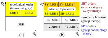
Figure 1: (Color online) (a) The possible gapped phases for a class of Hamiltonians $H(g_{1},g_{2})$ without any symmetry restriction. (b) The possible gapped phases for the class of Hamiltonians $H_{\text{symm}}(g_{1},g_{2})$ with symmetry. Each phase is labeled by its entanglement properties and symmetry breaking properties. SRE stands for short range entanglement, LRE for long range entanglement, SB for symmetry breaking, SY for no symmetry breaking. SB-SRE phases are the Landau symmetry breaking phases, which are understood by introducing group theory. The SY-SRE phases are the SPT phases, and we will show that they can be understood by introducing group cohomology theory. The SY-LRE phases are the SET phases.

Since its discovery, we have been trying to obtain a systematic and deeper understanding of topological orders. The studies of entanglement entropy show signs that topological orders are related to long-range entanglements.KP0604 ; LW0605 Recently, we found that topological orders actually can be regarded as patterns of long range entanglementsCGW1038 defined through local unitary (LU) transformations.LW0510 ; VCL0501 ; V0705

The notion of topological orders and long range entanglements leads to the following more general and more systematic picture of phases and phase transitions (see Fig. 1).CGW1038 For gapped quantum systems without any symmetry, their quantum phases can be divided into two classes: short range entangled (SRE) states and long range entangled (LRE) states.

SRE states are states that can be transformed into direct product states via LU transformations. All SRE states can be transformed into each other via LU transformations. So all SRE states belong to the same phase (see Fig. 1a).

LRE states are states that cannot be transformed into direct product states via LU transformations. It turns out that, many LRE states also cannot be transformed into each other. The LRE states that are not connected via LU transformations belong to different classes and represent different quantum phases. Those different quantum phases are nothing but the topologically ordered phases. Fractional quantum Hall statesTSG8259 ; L8395 , chiral spin liquids,KL8795 ; WWZ8913 $Z_{2}$ spin liquids,RS9173 ; W9164 ; MS0181 non-Abelian fractional quantum Hall states,MR9162 ; W9102 ; WES8776 ; RMM0899 etc are examples of topologically ordered phases. The mathematical foundation of topological orders is closely related to tensor category theoryFNS0428 ; LW0510 ; CGW1038 ; GWW1017 and simple current algebra.MR9162 ; LWW1024

For gapped quantum systems with symmetry, the structure of phase diagram is even richer (see Fig. 1b). Even SRE states now can belong to different phases. The Landau symmetry breaking states belong to this class of phases. However, there are more interesting examples in this class. Even SRE states that do not break any symmetry and have the same symmetry can belong to different phases. The 1D Haldane phases for spin-1 chainH8364 ; AKL8877 and topological insulatorsKM0501 ; BZ0602 ; KM0502 ; MB0706 ; FKM0703 ; QHZ0824 are examples of non-trivial SRE phases that do not break any symmetry. Those phases are beyond Landau symmetry breaking theory since they do not break any symmetry. We will call those phases Symmetry Protected Topological (SPT) phases.

For gapped quantum systems with symmetry, the corresponding LRE phases will be much richer than those without symmetry. We may call those phases Symmetry Enriched Topological (SET) phases. Projective symmetry group (PSG) was introduced to study the SET phases.W0213 ; W0303a Many examples of this kind of states can be found in LABEL:W0213,KLW0834,KW0906,LS0903,YFQ1070, but a systematic understanding is still lacking.

I.2 Motivation

The notion of topological order and long range entanglements deepens our understanding of quantum phases and guides our research strategy. This allows us to make significant progress.

For example, there is no long range entanglement in gapped 1D states.VCL0501 ; CGW1107 So, without symmetry, all gapped 1D quantum states belong to the same phase. For systems with a certain symmetry, all gapped 1D phases are either SPT phases protected by symmetry or symmetry breaking states. Since both SPT phases and symmetry breaking states are short range entangled, it is easy to understand them. As a result, a complete classification of all 1D gapped bosonic/fermionic quantum phases for any symmetry can be obtained.CGW1107 ; SPC1032 ; CGW1123 ; PBT1039 (A special case of the above result, a classification of 1D fermionic systems with $T^{2}=1$ time reversal symmetry can also be found in LABEL:TPB1102,FK1103,CGW1123). Using the idea of LU transformations, we also developed a systematic and quantitative theory for non-chiral topological orders in 2D interacting boson and fermion systems.LW0510 ; CGW1038 ; GWW1017 We would like to mention that symmetry protected Berry phases have been used to study various topological phases.H1 ; H2

Motivated by the 1D classification result, in this paper and in LABEL:CLW1152 we would like to study SPT phases in higher dimensions. Since SPT phases are short range entangled, it is relatively easy to obtain a systematic understanding. (Another way to make the classification problem easier is to consider only free fermion systems which are classified by K-theory.K0886 ; SRF0825 ) In LABEL:CLW1152, we study some simple but highly non-trivial examples. Those non-trivial examples lead to the generic and systematic results discussed in this paper. Some other examples of 2D gapped SPT phases are given in LABEL:YK1065,CGW1107,LS0903,SPC1032,ML.

I.3 Summary of results

Using group theory, we can obtain a systematic understanding of symmetry breaking phases (or more precisely, short-range entangled symmetry breaking phases). In this paper, we will show that, using group cohomology theory, we can obtain a systematic understanding of short-range entangled symmetric phases of bosons/qubits, even with strong interactions. Those phases are called bosonic SPT phases. In particular, we have obtained the following results for bosonic systems:

1. From each element in $(1+d)$-Borel-cohomology group ${\cal H}^{1+d}[G,U_{T}(1)]$, we can construct a distinct SPT phase that respects the on-site symmetry $G$ in $d$-spatial dimensions. Here $G$ may contain anti-unitary time reversal transformation and ${\cal H}^{1+d}[G,U_{T}(1)]$ is introduced in appendix D. Note that ${\cal H}^{1+d}[G,U_{T}(1)]$ is an Abelian group that can be calculated from the symmetry group $G$. The identity element in ${\cal H}^{1+d}[G,U_{T}(1)]$ correspond to trivial SPT phases while other elements corresponds to non-trivial SPT phases. For example, ${\cal H}^{2}[SO(3),U(1)]=Z_{2}$. So a 1D integer spin chain with $SO(3)$ spin rotation symmetry (but no translation symmetry) has two kinds of SPT phases: one is the trivial $S=0$ phase and the other is the Haldane phase.H8364 ; AKL8877

2. The low energy effective theory of a SPT phase with symmetry $G$ is given by a topological non-linear $\sigma$-model that contains only a $2\pi$-quantized topological $\theta$-term. The $2\pi$-quantized topological $\theta$-term in $(d+1)$D is classified by ${\cal H}^{1+d}[G,U_{T}(1)]$ which generalizes the topological term for non-linear $\sigma$-model with continuous symmetry.

3. We argue that a $d$-dimensional non-trivial SPT phase has gapless boundary excitations or degenerate boundary states. The boundary degeneracy may come from spontaneous symmetry breaking or topological orders. This is similar to the holographic principle for intrinsic topological orders.H8285 ; Wedgerev The boundary excitations of the SPT phase are described by a non-linear $\sigma$-model with a non-local Lagrangian (NLL) term that generalizes the Wess-Zumino-Witten (WZW) termWZ7195 ; W8322 for continuous non-linear $\sigma$-models. In (1+1)D and for continuous symmetry group, it is shown that non-linear $\sigma$-model with WZW term is gapless which is described by Kac-Moody current algebra.W8322

4. The SPT phases that respect on-site symmetry $G$ and translation symmetry can be obtained in the following way: In $1$-dimension, those phases are labeled by ${\cal H}^{1}[G,U_{T}(1)]\times{\cal H}^{2}[G,U_{T}(1)]$.CGW1107 ; SPC1032 ; CGW1123 In $2$-dimension, they are labeled by ${\cal H}^{1}[G,U_{T}(1)]\times\Big{\{}{\cal H}^{2}[G,U_{T}(1)]\Big{\}}^{2}\times{\cal H}^{3}[G,U_{T}(1)]$. A partial result ${\cal H}^{1}[G,U_{T}(1)]\times\Big{\{}{\cal H}^{2}[G,U_{T}(1)]\Big{\}}^{2}$ was obtained in LABEL:CGW1107. In $3$-dimension, they are labeled by ${\cal H}^{1}[G,U_{T}(1)]\times\Big{\{}{\cal H}^{2}[G,U_{T}(1)]\Big{\}}^{3}\times\Big{\{}{\cal H}^{3}[G,U_{T}(1)]\Big{\}}^{3}\times{\cal H}^{4}[G,U_{T}(1)]$.

This paper is organized as the following: In section II, we list the bosonic SPT phases for many symmetry groups in dimension 0,1,2,3, and discuss some examples of those SPT phases. In section III, we give a brief review of local unitary transformations. In section IV, we discuss canonical form of the ground state wave function for SPT phases. In section V, we study on-site symmetry transformations that leave the canonical ground state wave function unchanged. In section VI, we construct the on-site symmetry transformations through the cocycles of the symmetry group. In section VII, we introduced topological non-linear $\sigma$-model and discuss their SPT phases. We also argue that the boundary states of the topological non-linear $\sigma$-model are gapless or degenerate if the symmetry is not explicitly broken. In section VIII, we construct and classify topological non-linear $\sigma$-model through the cocycles of the symmetry group. In section IX and X, we show that the ground states of the topological non-linear $\sigma$-model all have trivial intrinsic topological orders, and the same SPT order if constructed from equivalent cocycles. In section XI, we discuss the relation between the cocycles in the topological non-linear $\sigma$-model and the Berry’s phase. In section XII, we study SPT phases with both on-site and translation symmetries.

Symm. group	$d=0$	$d=1$	$d=2$	$d=3$
$Z_{2}^{T}$	$\mathbb{Z}_{1}$	$\mathbb{Z}_{2}$	$\mathbb{Z}_{1}$	$\mathbb{Z}_{2}$
$Z_{2}^{T}\times\text{trn}$	$\mathbb{Z}_{1}$	$\mathbb{Z}_{2}$	$\mathbb{Z}_{2}^{2}$	$\mathbb{Z}_{2}^{4}$
$Z_{n}$	$\mathbb{Z}_{n}$	$\mathbb{Z}_{1}$	$\mathbb{Z}_{n}$	$\mathbb{Z}_{1}$
$Z_{n}\times\text{trn}$	$\mathbb{Z}_{n}$	$\mathbb{Z}_{n}$	$\mathbb{Z}_{n}^{2}$	$\mathbb{Z}_{n}^{4}$
$U(1)$	$\mathbb{Z}$	$\mathbb{Z}_{1}$	$\mathbb{Z}$	$\mathbb{Z}_{1}$
$U(1)\times\text{trn}$	$\mathbb{Z}$	$\mathbb{Z}$	$\mathbb{Z}^{2}$	$\mathbb{Z}^{4}$
$U(1)\rtimes Z_{2}^{T}$	$\mathbb{Z}$	$\mathbb{Z}_{2}$	$\mathbb{Z}_{2}$	$\mathbb{Z}^{2}_{2}$
$U(1)\rtimes Z_{2}^{T}\times\text{trn}$	$\mathbb{Z}$	$\mathbb{Z}\times\mathbb{Z}_{2}$	$\mathbb{Z}\times\mathbb{Z}_{2}^{3}$	$\mathbb{Z}\times\mathbb{Z}_{2}^{8}$
$U(1)\times Z_{2}^{T}$	$\mathbb{Z}_{1}$	$\mathbb{Z}^{2}_{2}$	$\mathbb{Z}_{1}$	$\mathbb{Z}^{3}_{2}$
$U(1)\times Z_{2}^{T}\times\text{trn}$	$\mathbb{Z}_{1}$	$\mathbb{Z}^{2}_{2}$	$\mathbb{Z}_{2}^{4}$	$\mathbb{Z}_{2}^{9}$
$U(1)\rtimes Z_{2}$	$\mathbb{Z}_{2}$	$\mathbb{Z}_{2}$	$\mathbb{Z}\times\mathbb{Z}_{2}$	$\mathbb{Z}_{2}$
$U(1)\times Z_{2}$	$\mathbb{Z}\times\mathbb{Z}_{2}$	$\mathbb{Z}_{1}$	$\mathbb{Z}\times\mathbb{Z}^{2}_{2}$	$\mathbb{Z}_{1}$
$Z_{n}\rtimes Z_{2}^{T}$	$\mathbb{Z}_{n}$	$\mathbb{Z}_{2}\times\mathbb{Z}_{(2,n)}$	$\mathbb{Z}^{2}_{(2,n)}$	$\mathbb{Z}_{2}\times\mathbb{Z}^{2}_{(2,n)}$
$Z_{n}\times Z_{2}^{T}$	$\mathbb{Z}_{(2,n)}$	$\mathbb{Z}_{2}\times\mathbb{Z}_{(2,n)}$	$\mathbb{Z}^{2}_{(2,n)}$	$\mathbb{Z}_{2}\times\mathbb{Z}^{2}_{(2,n)}$
$Z_{n}\rtimes Z_{2}$	$\mathbb{Z}_{2}\times\mathbb{Z}_{(2,n)}$	$\mathbb{Z}_{(2,n)}$	$\mathbb{Z}_{n}\times\mathbb{Z}_{2}\times\mathbb{Z}_{(2,n)}$	$\mathbb{Z}^{2}_{(2,n)}$
$Z_{m}\times Z_{n}$	$\mathbb{Z}_{m}\times\mathbb{Z}_{n}$	$\mathbb{Z}_{(m,n)}$	$\mathbb{Z}_{m}\times\mathbb{Z}_{n}\times\mathbb{Z}_{(m,n)}$	$\mathbb{Z}^{2}_{(m,n)}$
$D_{2}\times Z_{2}^{T}=D_{2h}$	$\mathbb{Z}^{2}_{2}$	$\mathbb{Z}^{4}_{2}$	$\mathbb{Z}^{6}_{2}$	$\mathbb{Z}^{9}_{2}$
$Z_{m}\times Z_{n}\times Z_{2}^{T}$	$\mathbb{Z}_{(2,m)}\times\mathbb{Z}_{(2,n)}$	$\mathbb{Z}_{2}\times\mathbb{Z}_{(2,m)}\times\mathbb{Z}_{(2,n)}\times\mathbb{Z}_{(m,n)}$	$\mathbb{Z}^{2}_{(2,m,n)}\times\mathbb{Z}^{2}_{(2,m)}\times\mathbb{Z}^{2}_{(2,n)}$	$\mathbb{Z}_{2}\times\mathbb{Z}^{4}_{(2,m,n)}\times\mathbb{Z}^{2}_{(2,m)}\times\mathbb{Z}^{2}_{(2,n)}$
$SU(2)$	$\mathbb{Z}_{1}$	$\mathbb{Z}_{1}$	$\mathbb{Z}$	$\mathbb{Z}_{1}$
$SO(3)$	$\mathbb{Z}_{1}$	$\mathbb{Z}_{2}$	$\mathbb{Z}$	$\mathbb{Z}_{1}$
$SO(3)\times\text{trn}$	$\mathbb{Z}_{1}$	$\mathbb{Z}_{2}$	$\mathbb{Z}\times\mathbb{Z}_{2}^{2}$	$\mathbb{Z}^{3}\times\mathbb{Z}_{2}^{3}$
$SO(3)\times Z_{2}^{T}$	$\mathbb{Z}_{1}$	$\mathbb{Z}_{2}^{2}$	$\mathbb{Z}_{2}$	$\mathbb{Z}_{2}^{3}$
$SO(3)\times Z_{2}^{T}\times\text{trn}$	$\mathbb{Z}_{1}$	$\mathbb{Z}_{2}^{2}$	$\mathbb{Z}_{2}^{5}$	$\mathbb{Z}_{2}^{12}$

Table 1: (Color online) SPT phases of interacting bosonic systems in $d$-spatial dimensions protected by on-site symmetry $G$. In absence of translation symmetry, the above table lists ${\cal H}^{1+d}[G,U_{T}(1)]$ whose elements label the SPT phases. Here $\mathbb{Z}_{1}$ means that our construction only gives rise to the trivial phase. $\mathbb{Z}_{n}$ means that the constructed non-trivial SPT phases plus the trivial phase are labeled by the elements in $\mathbb{Z}_{n}$. $Z_{2}^{T}$ represents time reversal symmetry, “trn” represents translation symmetry, $U(1)$ represents $U(1)$ symmetry, $Z_{n}$ represents cyclic symmetry, etc . Also $(m,n)$ is the greatest common divisor of $m$ and $n$. The red rows are for bosonic topological insulators and the blue rows bosonic topological superconductors. The red/blue rows without translation symmetry correspond to strong bosonic topological insulators/superconductors and the red/blue rows with translation symmetry also contain weak bosonic topological insulators/superconductors.

II Examples of bosonic SPT phases

In table 1, we list the SPT phases for some simple symmetry groups. In the following, we discuss some of those phases in detail. We also give some simple examples for some of the listed SPT states.

II.1 $SO(3)$ SPT states

For integer spin systems with the full $SO(3)$ spin rotation symmetries, the symmetry group is $SO(3)$. From ${\cal H}^{1+d}[SO(3),U(1)]$, we find one non-trivial SPT phase in 1D and infinite many in 2D. Those 2D SPT phases labeled by $k\in\mathbb{Z}$ have a special property that they can be described by continuous non-linear $\sigma$-model with $2\pi$-quantized topological $\theta$-term:

$$S =\int\hskip 1.0pt\mathrm{d}\tau\hskip 1.0pt\mathrm{d}^{2}x\;\big{(}\frac{1}{2\rho}{\rm Tr}(\partial_{\mu}g^{\dagger}\partial_{\mu}g)$$ (1)

$$\ \ \ \ \ \ \ \ +\hskip 1.0pt\mathrm{i}\hskip 1.0pt\frac{\theta}{2\pi^{2}}\frac{\epsilon^{\mu\nu\lambda}}{6}\frac{1}{8}{\rm Tr}[(g^{-1}\partial_{\mu}g)(g^{-1}\partial_{\nu}g)(g^{-1}\partial_{\lambda}g)]\Big{)},$$

where $g(\bm{x},t)$ is a $3\times 3$ matrix in $SO(3)$ and $\theta=2\pi k$, $k\in\mathbb{Z}$. This is because the topological term, when $k=0$ mod 4,LWwzw

$$\int\hskip 1.0pt\mathrm{d}\tau\hskip 1.0pt\mathrm{d}^{2}x\;\frac{k}{2\pi^{2}}\frac{\epsilon^{\mu\nu\lambda}}{6}\frac{1}{8}{\rm Tr}[(g^{-1}\partial_{\mu}g)(g^{-1}\partial_{\nu}g)(g^{-1}\partial_{\lambda}g)]$$ (2)

corresponds to ${\cal H}^{3}[SO(3),U(1)]$ whose elements are labeled by $k/4\in\mathbb{Z}$.

At the boundary, the topological term reduces to the well known WZW term which gives rise to gapless edge excitations.W8322 We would like to point out that $g^{-1}(\partial_{\mu}g)$ and $(\partial_{\mu}g)g^{-1}$ create excitations on the edge that move in the opposite directions. Since the $SO(3)$ symmetry acts as $g(x,t)\to hg(x,t)$, $h\in SO(3)$, only $(\partial_{\mu}g)g^{-1}$ carries non trivial $SO(3)$ quantum numbers while $g^{-1}(\partial_{\mu}g)$ is a $SO(3)$ singlet. So on the edge, the excitations with non-trivial $SO(3)$ quantum numbers all move in one direction, which breaks the time reversal and parity symmetry. In fact, under time reversal or parity transformations, $\theta\to-\theta$ and $k\to-k$.

In the above example, we see that a $2\pi$-quantized topological $\theta$-terms in a non-linear $\sigma$-model gives rise to a non-trivial SPT phase. However, the topological $\theta$-terms in continuous non-linear $\sigma$-model do not always correspond to non-trivial SPT phases. For example, $\pi_{2}(SO(3))=0$ and the continuous $SO(3)$ non-linear $\sigma$-model has no topological $\theta$-terms in (1+1)D. But we do have a 1D non-trivial SPT phase protected by $SO(3)$ symmetry. Also, $\pi_{4}(SO(3))=\mathbb{Z}_{2}$ and the continuous $SO(3)$ non-linear $\sigma$-model has non-trivial topological $\theta$-term in (3+1)D. But such topological $\theta$-term cannot produce non-trivial SPT phase protected by $SO(3)$ symmetry, since the topological term becomes trivial once we include the cut-off. In this paper, we will show that non-trivial $2\pi$-quantized topological $\theta$-terms can even be defined for lattice non-linear $\sigma$-models on discretized space-time. It is the $2\pi$-quantized topological $\theta$-terms in lattice non-linear $\sigma$-models that give rise to non-trivial SPT phases.

It is also possible that the above $SO(3)$ SPT phases labeled by $k$ and $k+1$ are connected by a continuous phase transition that do not break any symmetry. The gapless critical point is likely to be described by eqn. (1) with $\theta=2\pi(k+\frac{1}{2})$. When $\theta<2\pi(k+\frac{1}{2})$, it may flow to $2\pi k$ at low energies and when $\theta>2\pi(k+\frac{1}{2})$, it may flow to $2\pi(k+1)$. Since all the SPT phases are described by $2\pi$-quantized topological $\theta$-terms in lattice non-linear $\sigma$-models, the above picture about the transitions between SPT phases may be valid for generic SPT phases.

For integer spin systems with time reversal and the full $SO(3)$ spin rotation symmetries, the symmetry group is $SO(3)\times Z_{2}^{T}$. From ${\cal H}^{1+d}[SO(3)\times Z_{2}^{T},U_{T}(1)]$, we find one non-trivial SPT phase in 2D and seven in 3D. Note that on systems with boundary, the topological $\theta$-term in eqn. (1) breaks the time reversal symmetry. So we cannot use those $\mathbb{Z}$ classified topological $\theta$-terms to produce 2D SPT phases with time reversal and $SO(3)$ spin rotation symmetries. As a result, the 2D SPT phases with time reversal and $SO(3)$ spin rotation symmetries are only described by $\mathbb{Z}_{2}$.

II.2 $SU(2)$ SPT states

For bosonic systems with $SU(2)$ symmetry, the SPT phases are labeled by ${\cal H}^{1+d}[SU(2),U(1)]$. We find infinite many non-trivial $SU(2)$ SPT phases in $(2+4n)$ spatial dimension. Those $SU(2)$ SPT phases labeled by $k\in\mathbb{Z}$. There is no non-trivial $SU(2)$ SPT phase in other dimensions. Similarly, those $SU(2)$ SPT phases in 2-dimensions can be described by continuous non-linear $\sigma$-model with $2\pi$-quantized topological $\theta$-term:

$$S =\int\hskip 1.0pt\mathrm{d}\tau\hskip 1.0pt\mathrm{d}^{2}x\;\big{(}\frac{1}{2\rho}{\rm Tr}(\partial_{\mu}g^{\dagger}\partial_{\mu}g)$$ (3)

$$\ \ \ \ \ \ \ \ +\hskip 1.0pt\mathrm{i}\hskip 1.0pt\frac{\theta}{2\pi^{2}}\frac{\epsilon^{\mu\nu\lambda}}{6}\frac{1}{2}{\rm Tr}[(g^{-1}\partial_{\mu}g)(g^{-1}\partial_{\nu}g)(g^{-1}\partial_{\lambda}g)]\Big{)},$$

where $g(\bm{x},t)$ is a $2\times 2$ matrix in $SU(2)$ and $\theta=2\pi k$, $k\in\mathbb{Z}$.

II.3 $U(1)$ SPT states

From ${\cal H}^{1+d}[U(1),U(1)]=\mathbb{Z}$ for even $d$ and ${\cal H}^{1+d}[U(1),U(1)]=\mathbb{Z}_{1}$ for odd $d$, we find that spin/boson systems with $U(1)$ on-site symmetry have infinite non-trivial SPT phases labeled by non-zero integer in $d$ = even dimensions. This generalizes a result obtained by Levin for $d=2$.ML We note that ${\cal H}^{3}[SU(2),U(1)]={\cal H}^{3}[U(1),U(1)]=\mathbb{Z}$. The SPT states with $SU(2)$ symmetry can also be viewed as SPT states with $U(1)$ symmetry. We know that an $SU(2)$ SPT state labeled by $k\in\mathbb{Z}$ is described by eqn. (3) with $\theta=2\pi k$. Such an $SU(2)$ SPT state is also an non-trivial $U(1)$ SPT state labeled by $k\in\mathbb{Z}$.

We like to point out that it is believed that all 2D gapped phases with Abelian statistics are classified by $K$-matrix and the related $U(1)$ Chern-Simons theory.BW9045 ; R9002 ; WZ9290 All the quasiparticles in the 2D SPT phases are bosons. So the SPT phases are also described by $K$-matrices. We just need to find a way to include symmetry in the $K$-matrix approach, which is done in LABEL:LS0903. In particular, Michael LevinLU1 pointed out that a 2D $U(1)$ SPT phase can be described by a $U(1)\times U(1)$ Chern-Simons theory (or a double-layer quantum Hall state) (see also LABEL:LS,LV)

$${\cal L}=\frac{1}{4\pi}K_{IJ}a_{I\mu}\partial_{\nu}a_{J\lambda}\epsilon^{\mu\nu\lambda}+\frac{1}{2\pi}q_{I}A_{\mu}\partial_{\nu}a_{I\lambda}\epsilon^{\mu\nu\lambda}+...$$ (4)

with the $K$-matrix and the charge vector $\bm{q}$:BW9045 ; R9002 ; WZ9290

$$K=\begin{pmatrix}0&1\\ 1&2k\\ \end{pmatrix},\ \ \ \ \bm{q}=\begin{pmatrix}1\\ 1\\ \end{pmatrix}.$$ (5)

We note that such a $K$-matrix has two null vectors $\bm{n}_{1}=\begin{pmatrix}1\\ k\\ \end{pmatrix},\bm{n}_{2}=\begin{pmatrix}0\\ 1\\ \end{pmatrix}$ that satisfy $\bm{n}_{i}^{T}K^{-1}\bm{n}_{i}=0$. The null vectors correspond to quasiparticles with Bose statistics. Such null vectors would destabilize the state if we did not have the $U(1)$ symmetry, since we could include one of the corresponding quasiparticle operators in the Hamiltonian which would gap the edge excitations.Hsta In the presence of $U(1)$ symmetry, the quasiparticles carry $U(1)$ charges $\bm{q}^{T}K^{-1}\bm{n}_{1}=1-k$ and $\bm{q}^{T}K^{-1}\bm{n}_{2}=1$. We see that when $k\neq 1$, both quasiparticles that correspond to the null vectors carry non-zero $U(1)$ charges. Thus, the quasiparticle operators cannot be included in the Hamiltonian, and they do not gap the gapless edge excitations. The correspond state will have $U(1)$ protected gapless excitation and correspond to a non-trivial $U(1)$ SPT state. We see that the $K$-matrix and the charge vector $\bm{q}$ describe a non-trivial $U(1)$ SPT state when $k\neq 1$ and a trivial state when $k=1$. The 2D $U(1)$ SPT states are labeled by an integer.

II.4 Bosonic topological insulators/superconductors

The $U(1)\rtimes Z_{2}^{T}$ line in Table 1 describes the SPT phases for interacting bosons with time reversal symmetry $Z_{2}^{T}$ and boson number conservation (symmetry group = $U(1)\rtimes Z_{2}^{T}$, where time reversal $T$ and $U(1)$ transformations $U_{\theta}$ satisfy $TU_{\theta}=U_{-\theta}T$). Those phases are bosonic analogues of free fermion topological insulators protected by the same symmetry. From ${\cal H}^{1+d}[U(1)\rtimes Z_{2}^{T},U(1)]$, we find one kind of non-trivial bosonic topological insulators in 1D or 2D, and three kinds in 3D. The only non-trivial topological insulator in 1D is the same as the Haldane phase.

The $Z_{2}^{T}$ line in Table 1 describes interacting bosonic analogues of free fermion topological superconductorsSMF9945 ; RG0067 ; R0664 ; QHR0901 ; SF0904 with only time reversal symmetry, $Z_{2}^{T}$ . Since ${\cal H}^{1+d}[Z_{2}^{T},U(1)]=\mathbb{Z}_{2}$ for odd $d$ and ${\cal H}^{1+d}[Z_{2}^{T},U(1)]=\mathbb{Z}_{1}$ for even $d$, we find one kind of “bosonic topological superconductors” or non-trivial SPT phases in every odd dimensions (for the spin/boson systems with only time reversal symmetry).

II.5 Other SPT states

The $U(1)\times Z_{2}^{T}$ line describes the SPT phases for integer spin systems with time reversal and $U(1)$ spin rotation symmetries (symmetry group = $U(1)\times Z_{2}^{T}$, where time reversal $T$ and $U(1)$ transformations $U_{\theta}$ satisfy $TU_{\theta}=U_{\theta}T$). From ${\cal H}^{1+d}[U(1)\times Z_{2}^{T},U(1)]$, we find three non-trivial SPT phases in 1D, none in 2D, and seven in 3D.

We also find that ${\cal H}^{1+d}[Z_{n},U(1)]=\mathbb{Z}_{n}$ for even $d$ and ${\cal H}^{1+d}[Z_{n},U(1)]=\mathbb{Z}_{1}$ for odd $d$. So spin/boson systems with $Z_{n}$ on-site symmetry have $n-1$ kinds of non-trivial SPT phases in $d$ = even dimensions.

For integer spin systems with $D_{2h}$ symmetry but no translation symmetry, we discover $15$ new SPT phases in 1D,CGW1123 ; LCW1121 $63$ new SPT phases in 2D, and $511$ new SPT phases in 3D.

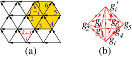
Figure 2: (a) A triangular lattice. The Hamiltonian term (II.6) acts on the seven sites in the shaded area. (b) A geometric representation of the the phase factors in eqn. (II.6).

II.6 Ideal ground state wave functions and exactly soluble Hamiltonians for SPT phases

We can construct the idea ground state wave functions and exactly soluble Hamiltonians for all the SPT phases described by ${\cal H}^{1+d}[G,U_{T}(1)]$. The elements in ${\cal H}^{1+d}[G,U_{T}(1)]$ are complex functions of $d+2$ variables $\nu_{d+1}(g_{0},...,g_{d+1})$, $g_{i}\in G$. $\nu_{d+1}(g_{0},...,g_{d+1})$ is a pure phase $|\nu_{d+1}(g_{0},...,g_{d+1})|=1$ that satisfy certain cocycle conditions (16) and (17). From each element $\nu_{d+1}(g_{0},...,g_{d+1})$ we can construct the $d$-dimensional ground state wave function for the corresponding SPT phase. In 2D, we can start with a triangle lattice model where the physical states on site-$i$ are given by $|g_{i}\rangle$, $g_{i}\in G$ (see Fig. 2a). The ideal ground state wave function is then given by $\Phi(\{g_{i}\})=\prod_{\bigtriangleup}\nu_{3}(1,g_{i},g_{j},g_{k})\prod_{\bigtriangledown}\nu_{3}^{-1}(1,g_{i},g_{j},g_{k})$, where $\prod_{\bigtriangleup}$ and $\prod_{\bigtriangledown}$ multiply over all up- and down-triangles, and the order of $ijk$ is clockwise for up-triangles and anti-clockwise for down-triangles (see Fig. 2a).

To construct exactly soluble Hamiltonian $H$ that realizes the above wave function as the ground state, we start with an exactly soluble Hamiltonian $H_{0}=-\sum_{i}|\phi_{i}\rangle\langle\phi_{i}|$, $|\phi_{i}\rangle=\sum_{g_{i}\in G}|g_{i}\rangle$, whose ground state is $\Phi_{0}(\{g_{i}\})=1$. Then, using the local unitary transformation $U=\prod_{\bigtriangleup}\nu_{3}(1,g_{i},g_{j},g_{k})\prod_{\bigtriangledown}\nu_{3}^{-1}(1,g_{i},g_{j},g_{k})$, we find that the above ideal ground state wave function is given by $\Phi=U\Phi_{0}$ and the corresponding exactly soluble Hamiltonian is given by $H=\sum_{i}H_{i}$, where $H_{i}=U|\phi_{i}\rangle\langle\phi_{i}|U^{\dagger}$. $H_{i}$ acts on a seven-spin cluster labeled by $i$, 1 – 6 in shaded area in Fig. 2a

$$H_{i}|g_{i},g_{1}g_{2}g_{3}g_{4}g_{5}g_{6}\rangle=\sum_{g_{i}^{\prime}}|g_{i}^{\prime},g_{1}g_{2}g_{3}g_{4}g_{5}g_{6}\rangle\times$$

$$\ \ \ \ \ \ \ \frac{\nu_{3}(g_{4},g_{5},g_{i},g_{i}^{\prime})\nu_{3}(g_{5},g_{i},g_{i}^{\prime},g_{6})\nu_{3}(g_{i},g_{i}^{\prime},g_{6},g_{1})}{\nu_{3}(g_{i},g_{i}^{\prime},g_{2},g_{1})\nu_{3}(g_{3},g_{i},g_{i}^{\prime},g_{2})\nu_{3}(g_{4},g_{3},g_{i},g_{i}^{\prime})}$$ (6)

The above phase factor has a graphic representation as in Fig. 2b. (For a detailed explanation of the graphic representation see Fig. 10.) $H$ has a short ranged interaction and has the symmetry $G$: $|\{g_{i}\}\rangle\to|\{gg_{i}\}\rangle,\ g\in G$, if $\nu_{3}(g_{0},...,g_{3})$ satisfies the 3-cocycle conditions eqn. (16) and eqn. (20).

For symmetry $G=Z_{2}$ and using the 3-cocycle calculated in section J.2, we find that the Hamiltonian that realize the non-trivial $Z_{2}$ SPT state in two dimensions is given by

$$H_{i}=\sigma^{+}_{i}\eta^{+}_{21}\eta^{+}_{32}\eta^{+}_{43}\eta^{+}_{45}\eta^{+}_{56}\eta^{+}_{61}+\sigma^{-}_{i}\eta^{-}_{21}\eta^{-}_{32}\eta^{-}_{43}\eta^{-}_{45}\eta^{-}_{56}\eta^{-}_{61}$$ (7)

where

$$\sigma^{+}_{i}=\begin{pmatrix}0&0\\ 1&0\\ \end{pmatrix},\ \ \ \ \ \sigma^{-}_{i}=\begin{pmatrix}0&1\\ 0&0\\ \end{pmatrix},$$ (8)

which act on site-$i$. Also $\eta^{\pm}_{ij}$ are operators acting on site-$i$ and site-$j$:

$$\eta^{+}_{ij}|0\rangle_{i}\otimes|1\rangle_{j}=-|0\rangle_{i}\otimes|1\rangle_{j},$$

$$\eta^{+}_{ij}|\alpha\rangle_{i}\otimes|\beta\rangle_{j}=|\alpha\rangle_{i}\otimes|\beta\rangle_{j},\ \ \ (\alpha,\beta)\neq(0,1)$$

$$\eta^{-}_{ij}|1\rangle_{i}\otimes|0\rangle_{j}=-|1\rangle_{i}\otimes|0\rangle_{j},$$

$$\eta^{-}_{ij}|\alpha\rangle_{i}\otimes|\beta\rangle_{j}=|\alpha\rangle_{i}\otimes|\beta\rangle_{j},\ \ \ (\alpha,\beta)\neq(1,0).$$ (9)

II.7 A classification of short-range-entangled states with or without symmetry breaking

The above results are for bosonic states that do not break any symmetry of the Hamiltonian. Combining group theory (that describe the symmetry break states) and group cohomology theory (that describes the SPT states), we can obtain a theory for more general short-range-entangled states that may break the symmetry $G_{H}$ of the Hamiltonian down to the symmetry $G_{\Psi}$ of the ground states. We find that the different symmetry breaking short-range-entangled phases are described/labeled by the following three mathematical objects: $\Big{(}G_{H},G_{\Psi},{\cal H}^{1+d}[G_{\Psi},U_{T}(1)]\Big{)}$.

Landau symmetry breaking theory tries to use $(G_{H},G_{\Psi})$ to describe/label all the symmetry breaking short-range-entangled phases. We see that Landau symmetry breaking theory misses the third label ${\cal H}^{1+d}[G_{\Psi},U_{T}(1)]$. The SPT phases do not break any symmetry and are described by $\Big{(}G_{H},G_{H},{\cal H}^{1+d}[G_{H},U_{T}(1)]\Big{)}\sim{\cal H}^{1+d}[G_{H},U_{T}(1)]$.

III Local unitary transformations

In the rest of the paper, we will explain the ideas, the way of thinking, and the detailed calculations that allow us to obtain the results described in the above section. We will start with a short review of local unitary (LU) transformation.LW0510 ; VCL0501 ; V0705 ; CGW1038

LU transformation is an important concept which is directly related to the definition of quantum phases.CGW1038 In this section, we will explain what it is. Let us first introduce local unitary evolution. A LU evolution is defined as the following unitary operator that act on the degrees of freedom in a quantum system:

$${\cal T}[e^{-i\int_{0}^{1}dg\,\tilde{H}(g)}]$$ (10)

where ${\cal T}$ is the path-ordering operator and $\tilde{H}(g)=\sum_{\bm{i}}O_{\bm{i}}(g)$ is a sum of local Hermitian operators. Two gapped quantum states belong to the same phase if and only if they are related by a LU evolution.HW0541 ; BHM1044 ; CGW1038

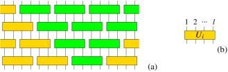
Figure 3: (Color online) (a) A graphic representation of a quantum circuit, which is form by (b) unitary operations on blocks of finite size $l$. The green shading represents a causal structure.

The LU evolutions is closely related to quantum circuits with finite depth. To define quantum circuits, let us introduce piecewise local unitary operators. A piecewise local unitary operator has a form

$$U_{pwl}=\prod_{i}U^{i}$$

where $\{U^{i}\}$ is a set of unitary operators that act on non overlapping regions. The size of each region is less than some finite number $l$. The unitary operator $U_{pwl}$ defined in this way is called a piecewise local unitary operator with range $l$. A quantum circuit with depth $M$ is given by the product of $M$ piecewise local unitary operators:

$$U^{M}_{circ}=U_{pwl}^{(1)}U_{pwl}^{(2)}\cdots U_{pwl}^{(M)}$$

We will call $U^{M}_{circ}$ a LU transformation. In quantum information theory, it is known that finite time unitary evolution with local Hamiltonian (LU evolution defined above) can be simulated with constant depth quantum circuit (ie a LU transformation) and vice-verse:

$${\cal T}[e^{-i\int_{0}^{1}dg\,\tilde{H}(g)}]=U^{M}_{circ}.$$ (11)

So two gapped quantum states belong to the same phase if and only if they are related by a LU transformation.

In this paper, we will use the LU transformations to simplify gapped quantum states within the same phase. This allows us to gain a deeper understanding and even to classify gapped quantum phases.

IV Canonical form of many-body states with short range entanglements

A generic many-body wave function $\Phi(m_{1},...,m_{N})$ is very complicated. It is hard to see and identify the quantum phase represented by a many-body wave function. In this section, we will use LU transformations to simplify many-body wave functions in order to understand the structure of quantum phases.

Such an approach is very effective in 1DCGW1107 ; SPC1032 ; CGW1123 which leads to a complete classification of gapped 1D phases. In two dimensions, the approach allows us to classify non-chiral topological orders.LW0510 ; CGW1038 ; GWW1017 In this paper, we will study another problem where such an approach is effective. We will use LU transformations to study SRE quantum phases with symmetries and study SPT phases that do not break any symmetry.

IV.1 Cases without any symmetry

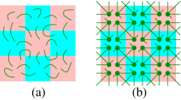
Figure 4: (Color online) Transforming a SRE state to a tensor-network state which take simple canonical form. (a) A SRE state. (b) Using the unitary transformations that act within each block, we can transform the SRE state to a tensor-network state. Entanglements exist only between the degrees of freedom on the connected tensors.

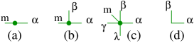
Figure 5: (Color online) Graphic representations of tensors: (a) $A^{m}_{\alpha}$, (b) $A^{m}_{\alpha\beta}$, and (c) $A^{m}_{\alpha\beta\gamma\lambda}$. (d) A corner represents a special rank-2 tensor $A_{\alpha\beta}=\delta_{\alpha\beta}$.

Without any symmetry, we can always use LU transformations to transform a SRE wave function into a product state. In the following, we will describe how to choose such LU transformation and what is the form of the resulting product state.

We first divide our system into patches of size $l$ as in Fig. 4a. If $l$ is large enough, entanglement only exists between regions that share an edge or a corner. In this case, we can use LU transformation to transform the state in Fig. 4a into a state with many unentangled regions (see Fig. 4b). For example, some degrees of freedom in the middle square in Fig. 4a may be entangled with the degrees of freedom in the three squares below, to the right, and to the lower-right of the middle square. We can use the LU transformation inside the middle square to move all those degrees of freedom to the lower-right corner of the middle square. Similarly, we can use the LU transformation to move all the degrees of freedom that are entangled with the three squares below, to the left, and to the lower-left of the middle square to the lower-left corner of the middle square, etc. Repeat such operation to every square and we obtain a state described by Fig. 4b. For stabilizer states, such reduction procedure has been established explicitly.SB

Fig. 4b is a graphic representation of a tensor-network description of the state.GMN0391 ; NMG0415 ; M0460 ; VC0466 ; JOV0802 ; GLWtergV ; JWX0803 In the graphic representation, a dot with $n$ legs represents a rank $n$ tensor (see Fig. 5). If two legs are connected, the indexes on those legs will take the same value and are summed over. In the tensor-network representation of states, we can see the entanglement structure. The disconnected parts of tensor-network are not entangled. In particular, the tensor-network state Fig. 4b is a direct product state.

If there is no symmetry, we can transform any direct product state to any other direct product state via LU transformations. So all SRE states belong to one phase.

IV.2 Cases with an on-site symmetry

However, when we study phases of systems with certain symmetry, we can only use the LU transformations that respect the symmetry to connect states within the same phase. In this case, even SRE states with the same symmetry can belong to different phases.

Let us consider $d$-dimensional systems of $N$ sites that have only an on-site symmetry group $G$. We also assume that the states $|m\rangle$ on each site form a linear representation $U_{mm^{\prime}}(g),\ g\in G$ of the group $G$.

To understand the structure of quantum phases of the symmetric states that do not break the symmetry $G$, we can only use symmetric LU transformation that respects the on-site symmetry $G$ to define phases. Two gapped symmetric states are in the same phase if and only if they can be connected by a symmetric LU transformation.CGW1038

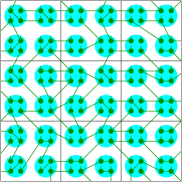
Figure 6: (Color online) A tensor network representation of a SRE state with on-site symmetry $G$. The all the dots in each shaded circle form a site. The degrees of freedom on each site (ie in each shaded circle) form a linear representation of $G$. However, the degrees of freedom on each dot may not form a linear representation of $G$.

We have argued that generic LU transformations can change a SRE state in Fig. 4a to a tensor-network state in Fig. 4b. The LU transformations rearrange the spatial distributions of the entanglements which should not be affected by the on-site symmetry $G$. So, in the following, we would like to argue that symmetric LU transformations can still change a SPT state in Fig. 4a to a symmetric tensor-network state in Fig. 4b (although a generic proof is missing).

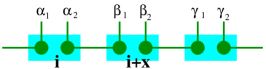
Figure 7: (Color online) The canonical tensor network representation for 1D SRE state $|\Psi_{\text{pSRE}}\rangle$. The two dots in each rectangle represent a physical site.

We first assume that symmetric SRE states have tensor network representation as shown in Fig. 6. The linked dots represent the entangled degrees of freedom. The dots in each shaded circle represent a site, which forms a linear representation of the on-site symmetry group $G$. We then divide the systems into large squares (see Fig. 6). The size of the square is large enough such that entanglement only appears between squares that share an edge or a vertex. Now we view the degrees of freedom in each square as a large effective site. The degrees of freedom on each effective site form a linear representation of $G$. Now, we can use an unitary transformation in each square to rearrange the degrees of freedom in that square (which corresponds to change basis in the large effective site). This way, we can transform the SPT state in Fig. 6 into the canonical form in Fig. 4b, where the degrees of freedom on each shaded square form a linear representation of $G$. So Fig. 4b is a symmetric tensor-network state. We would like to point out that although in Fig. 4b, we only present a 2D tensor-network state in canonical form, the similar reduction can be done in any dimensions.

V Classify symmetry transformations of SPT states

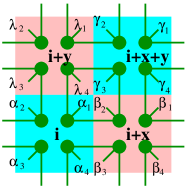
Figure 8: (Color online) The canonical tensor network representation for 2D SRE state $|\Psi_{\text{pSRE}}\rangle$. The four dots in each square represent a physical site.

After the symmetric state being reduced to the canonical form in Fig. 4b, the on-site symmetry transformation is generated by the following matrix on the effective site-$\bm{i}$: $U^{\bm{i}}_{\alpha_{1}\alpha_{2}\alpha_{3}\alpha_{4},\alpha_{1}^{\prime}\alpha_{2}^{\prime}\alpha_{3}^{\prime}\alpha_{4}^{\prime}}$ which forms a linear representation of the on-site symmetry group $G$. The symmetry transformation $U^{\bm{i}}_{\alpha_{1}\alpha_{2}\alpha_{3}\alpha_{4},\alpha_{1}^{\prime}\alpha_{2}^{\prime}\alpha_{3}^{\prime}\alpha_{4}^{\prime}}$ keeps the SRE state $|\Psi_{\text{pSRE}}\rangle$ in Fig. 7 or Fig. 8 invariant:

$$\otimes_{\bm{i}}U^{\bm{i}}|\Psi_{\text{pSRE}}\rangle=|\Psi_{\text{pSRE}}\rangle$$ (12)

for any lattice size.

Eqn. (12) is one of the key equations. It describes the condition that the on-site symmetry transformations $U^{\bm{i}}$ must satisfy so that those on-site symmetry transformations can represent the symmetry of a SRE state. So to classify all possible symmetry transformations of SPT states, we need to find all the pairs $(U^{\bm{i}},|\Psi_{\text{pSRE}}\rangle)$ that satisfy eqn. (12). Those different solutions can correspond to different SRE symmetric phases.

However, two different solutions $U^{\bm{i}}$ may not correspond to different phases. They may be “equivalent” and can correspond to the same phase. So to understand the structure of SRE symmetric phases, we also need to find out those “equivalent” relations. Clearly one “equivalent” relation is generated by unitary transformations $W^{\bm{i}}_{\alpha_{1}\alpha_{2}\alpha_{3}\alpha_{4},\beta_{1}\beta_{2}\beta_{3}\beta_{4}}$ on each effective physical site:

$$\ \ \ U^{\bm{i}}_{\alpha_{1}\alpha_{2}\alpha_{3}\alpha_{4},\alpha_{1}^{\prime}\alpha_{2}^{\prime}\alpha_{3}^{\prime}\alpha_{4}^{\prime}}\sim\tilde{U}^{\bm{i}}_{\alpha_{1}\alpha_{2}\alpha_{3}\alpha_{4},\alpha_{1}^{\prime}\alpha_{2}^{\prime}\alpha_{3}^{\prime}\alpha_{4}^{\prime}}$$ (13)

$$=W^{\bm{i}}_{\alpha_{1}\alpha_{2}\alpha_{3}\alpha_{4},\beta_{1}\beta_{2}\beta_{3}\beta_{4}}U^{\bm{i}}_{\beta_{1}\beta_{2}\beta_{3}\beta_{4},\beta_{1}^{\prime}\beta_{2}^{\prime}\beta_{3}^{\prime}\beta_{4}^{\prime}}W^{\bm{i}{\dagger}}_{\beta_{1}^{\prime}\beta_{2}^{\prime}\beta_{3}^{\prime}\beta_{4}^{\prime},\alpha_{1}^{\prime}\alpha_{2}^{\prime}\alpha_{3}^{\prime}\alpha_{4}^{\prime}}$$

where the repeated indices are summed over. Here $W^{\bm{i}}_{\alpha_{1}\alpha_{2}\alpha_{3}\alpha_{4},\beta_{1}\beta_{2}\beta_{3}\beta_{4}}$ are not the most general on-site unitary transformations. They are the on-site unitary transformations that map $|\Psi_{\text{pSRE}}\rangle$ to another state $|\Psi^{\prime}_{\text{pSRE}}\rangle$ having the same form as described by Fig. 7 or Fig. 8.

The second “equivalent” relation is given by

$$\ \ \ U^{\bm{i}}_{\alpha_{1}\alpha_{2}\alpha_{3}\alpha_{4},\alpha_{1}^{\prime}\alpha_{2}^{\prime}\alpha_{3}^{\prime}\alpha_{4}^{\prime}}\sim\tilde{U}^{\bm{i}}_{\alpha_{1}\beta_{1}\alpha_{2}\beta_{2}\alpha_{3}\beta_{3}\alpha_{4}\beta_{4},\alpha_{1}^{\prime}\beta_{1}^{\prime}\alpha_{2}^{\prime}\beta_{2}^{\prime}\alpha_{3}^{\prime}\beta_{3}^{\prime}\alpha_{4}^{\prime}\beta_{4}^{\prime}}$$

$$=U^{\bm{i}}_{\alpha_{1}\alpha_{2}\alpha_{3}\alpha_{4},\alpha_{1}^{\prime}\alpha_{2}^{\prime}\alpha_{3}^{\prime}\alpha_{4}^{\prime}}W^{1,\bm{i}}_{\beta_{1},\beta_{1}^{\prime}}W^{2,\bm{i}}_{\beta_{2},\beta_{2}^{\prime}}W^{3,\bm{i}}_{\beta_{3},\beta_{3}^{\prime}}W^{4,\bm{i}}_{\beta_{4},\beta_{4}^{\prime}}$$ (14)

where $W^{a,\bm{i}}_{\beta_{a},\beta_{a}^{\prime}}$, $a=1,2,3,4$ are linear representations of the on-site symmetry group $G$ which satisfy a condition that the direct product representation $W^{1,\bm{i}}\otimes W^{2,\bm{i}+\bm{x}}\otimes W^{3,\bm{i}+\bm{x}+\bm{y}}\otimes W^{4,\bm{i}+\bm{y}}$ contains a trivial 1D representation:

$$W^{1,\bm{i}}\otimes W^{2,\bm{i}+\bm{x}}\otimes W^{3,\bm{i}+\bm{x}+\bm{y}}\otimes W^{4,\bm{i}+\bm{y}}=1\oplus...$$ (15)

Such an “equivalent” relation arises from the fact that adding local degrees of freedom that form a 1D representation does not change the phase of state (see Fig. 9) It is clear that if the transformations $U^{\bm{i}}$ satisfy eqn. (12), $\tilde{U}^{\bm{i}}$ from the second “equivalent” relation also satisfy eqn. (12).

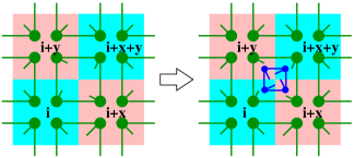
Figure 9: (Color online) Adding four local degrees of freedom that form a 1D representation does not change the phase of state.

The solutions of eqn. (12) can be grouped into classes using the equivalence relations eqn. (13) and eqn. (V). Those classes should correspond different SPT states.

We note that the condition eqn. (12) involves the whole many-body wave function. In appendix A, we will show that the condition eqn. (12) can be rewritten as a local condition where only a local region of the many-body wave function is used. Although we only discuss the 2D case in the above, similar result can be obtained in any dimensions.

The discussions in the last a few sections outline some ideas that may lead to a classification of SPT phases. In this paper, we will not attempt to directly find all the solutions of eqn. (12) and to directly classify all the SPT phases. Instead, we will try to explicitly construct, as general as possible, the solutions of eqn. (12). Our goal is to find a general construction that produces all the possible solutions.

VI Constructing SPT phases through group cocycles

In this section, we will construct solutions of eqn. (12) through the cocycles of the symmetry group $G$. The different solutions will correspond to different SPT phases.

VI.1 Group cocycles

The cocycles, cohomology group, and their graphic representations on simplex with branching structure are discussed in appendix D and E. Here we just briefly introduce those concepts. A $d$-cochain of group $G$ is a complex function $\nu_{d}(g_{0},g_{1},...,g_{d})$ of $1+d$ variables in $G$ that satisfy

$$|\nu_{d}(g_{0},g_{1},...,g_{d})| =1,$$ (16)

$$\nu_{d}^{s(g)}(g_{0},g_{1},...,g_{d}) =\nu_{d}(gg_{0},gg_{1},...,gg_{d}),\ \ g\in G$$

where $s(g)=1$ if $g$ contains no anti-unitary time reversal transformation $T$ and $s(g)=-1$ if $g$ contains one anti-unitary time reversal transformation $T$. [When $G$ is continuous, we do not require the cochain $\nu_{d}(g_{0},g_{1},...,g_{d})$ to be a continuous function of $g_{i}$. Rather, we only require $\nu_{d}(g_{0},g_{1},...,g_{d})$ to be a so called measurable function of $g_{i}$.MFun A measurable function is not continuous only on a measure zero space.]

The $d$-cocycles are special $d$-cochains that satisfy

$$\ \ \ \prod_{i=0}^{d+1}\nu_{d}^{(-1)^{i}}(g_{0},..,g_{i-1},g_{i+1},...,g_{d+1})=1.$$ (17)

For $d=1$, the 1-cocycles satisfy

$$\nu_{1}(g_{1},g_{2})\nu_{1}(g_{0},g_{1})/\nu_{1}(g_{0},g_{2})=1$$ (18)

The 2-cocycles satisfy

$$\frac{\nu_{2}(g_{1},g_{2},g_{3})\nu_{2}(g_{0},g_{1},g_{3})}{\nu_{2}(g_{0},g_{2},g_{3})\nu_{2}(g_{0},g_{1},g_{2})}=1$$ (19)

and the 3-cocycles satisfy

$$\frac{\nu_{3}(g_{1},g_{2},g_{3},g_{4})\nu_{3}(g_{0},g_{1},g_{3},g_{4})\nu_{3}(g_{0},g_{1},g_{2},g_{3})}{\nu_{3}(g_{0},g_{2},g_{3},g_{4})\nu_{3}(g_{0},g_{1},g_{2},g_{4})}=1$$ (20)

The $d$-coboundaries $\lambda_{d}$ are special $d$-cocycles that can be constructed from the $(d-1)$-cochains $\mu_{d-1}$:

$$\ \ \ \lambda_{d}(g_{0},...,g_{d})=\prod_{i=0}^{d}\mu_{d-1}^{(-1)^{i}}(g_{0},..,g_{i-1},g_{i+1},...,g_{d}).$$ (21)

For $d=1$, the 1-coboundaries are given by

$$\lambda_{1}(g_{0},g_{1})=\mu_{0}(g_{1})/\mu_{0}(g_{0})$$ (22)

The 2-coboundaries are given by

$$\lambda_{2}(g_{0},g_{1},g_{2})=\mu_{1}(g_{1},g_{2})\mu_{1}(g_{0},g_{1})/\mu_{1}(g_{0},g_{2}),$$ (23)

and the 3-coboundaries by

$$\lambda_{3}(g_{0},g_{1},g_{2},g_{3})=\frac{\mu_{2}(g_{1},g_{2},g_{3})\mu_{2}(g_{0},g_{1},g_{3})}{\mu_{2}(g_{0},g_{2},g_{3})\mu_{2}(g_{0},g_{1},g_{2})}.$$ (24)

Two $d$-cocycles, $\nu_{d}$ and $\nu^{\prime}_{d}$, are said to be equivalent iff they differ by a coboundary $\lambda_{d}$: $\nu_{d}=\nu^{\prime}_{d}\lambda_{d}$. The equivalence classes of cocycles give rise to the $d$-cohomology group ${\cal H}^{d}[G,U_{T}(1)]$.

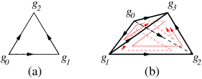
Figure 10: (Color online) (a) The line from $g_{0}$ to $g_{1}$ is a graphic representation of $\nu_{1}(g_{0},g_{1})$. The triangle $(g_{0},g_{1},g_{2})$ with a branching structure (see appendix E) is a graphic representation of $\nu_{2}(g_{0},g_{1},g_{2})$. Note that, for the first variable, the $g_{0}$-vertex is connected to two outgoing edges, and for the last variable, the $g_{2}$-vertex is connected to two incoming edges. (a) can also be viewed as the graphic representation of eqn. (18) and eqn. (130). The triangle corresponds to $(\hskip 1.0pt\mathrm{d}_{1}\nu_{1})(g_{0},g_{1},g_{2})$ in eqn. (130) and the three edges correspond to $\nu_{1}(g_{1},g_{2})$, $\nu_{1}(g_{0},g_{1})$ and $\nu_{1}^{-1}(g_{0},g_{2})$. (b) The tetrahedron $(g_{0},g_{1},g_{2},g_{3})$ with a branching structure is a graphic representation of $\nu_{3}(g_{0},g_{1},g_{2},g_{3})$. (b) can also be viewed as the graphic representation of eqn. (19) and eqn. (131). The tetrahedron corresponds to $(\hskip 1.0pt\mathrm{d}_{2}\nu_{2})(g_{0},g_{1},g_{2},g_{3})$ in eqn. (131), and the four faces correspond to $\nu_{2}(g_{1},g_{2},g_{3})$, $\nu_{2}(g_{0},g_{1},g_{3})$, $\nu_{2}^{-1}(g_{0},g_{2},g_{3})$, and $\nu_{2}^{-1}(g_{0},g_{1},g_{2})$.

A $d$-cochain can be represented by a $d$-dimensional simplex with a branching structure (see Fig. 10). A branching structure (see appendix E) is represented by arrows on the edges of the simplex that never form an oriented loop on any triangles. We note that the first variable $g_{0}$ in $\nu_{d}(g_{0},g_{1},...,g_{d})$ corresponds to the vertex with no incoming edge, the second variable $g_{1}$ to the vertex with one incoming edge, and the third variable $g_{2}$ to the vertex with two incoming edges, etc . The conditions eqn. (18) and eqn. (19) can also be represented as in Fig. 10. For example, Fig. 10a has three edges which correspond to $\nu_{1}(g_{1},g_{2})$, $\nu_{1}(g_{0},g_{1})$ and $\nu_{1}^{-1}(g_{0},g_{2})$. The evaluation of a $1$-cochain $\nu_{1}$ on the complex Fig. 10a is given by the product of the factors $\nu_{1}(g_{1},g_{2})$, $\nu_{1}(g_{0},g_{1})$ and $\nu_{1}^{-1}(g_{0},g_{2})$. Such an evaluation will be 1 if $\nu_{1}$ is a cocycle. In general, the evaluations of cocycles on any complex without boundary are 1.

Such a geometric picture will help us to obtain most of the results in this paper.

VI.2 (1+1)D case

Let us discuss the 1D case first. We will choose the 1D SPT wave function to have a fixed form of a “dimer crystal” (see Fig. 7):

$$|\Psi_{\text{pSRE}}\rangle =...\otimes(\sum_{g\in G}|\alpha_{2}=g,\beta_{1}=g\rangle)\otimes$$

$$(\sum_{g\in G}|\beta_{2}=g,\gamma_{1}=g\rangle)\otimes...$$ (25)

where we have assumed that physical states on each dot in Fig. 7 are labeled by the elements of the symmetry group $G$: $\alpha_{i},\beta_{i}\in G$. The dimmer in Fig. 7 corresponds to a maximally entangled state $\sum_{g\in G}|\alpha_{2}=g,\beta_{1}=g\rangle$.

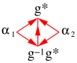
Figure 11: (Color online) The graphic representation of eqn. (27). $f_{2}(\alpha_{1},\alpha_{2},g,g^{*})$ is represented by the polygon with a branching structure as represented by the arrows on the edge which never form a oriented loop on any triangle. $\nu_{2}(\alpha_{1},g^{-1}g^{*},g^{*})$ and $\nu_{2}(\alpha_{2},g^{-1}g^{*},g^{*})$ are represented by the two triangles as in Fig. 10a. The value of the cocycle $\nu_{2}$ on a triangle (say $\nu_{2}(\alpha_{1},g^{-1}g^{*},g^{*})$) can be viewed as flux going through the corresponding triangle.

Next, we need to choose an on-site symmetry transformation (12) such that the state $|\Psi_{\text{pSRE}}\rangle$ is invariant (where the two dots in each shaded box represent a site). We note that $U^{\bm{i}}(g)$ acts on the states on the $\bm{i}$ site which are linear combinations of $|\alpha_{1},\alpha_{2}\rangle$ in Fig. 7. Note that $\alpha_{1},\alpha_{2}\in G$. So we can choose the action of $U^{\bm{i}}(g)$ to be (see Fig. 11)

$$U^{\bm{i}}(g)|\alpha_{1},\alpha_{2}\rangle=f_{2}(\alpha_{1},\alpha_{2},g,g^{*})|g\alpha_{1},g\alpha_{2}\rangle$$ (26)

where $f_{2}(\alpha_{1},\alpha_{2},g,g^{*})$ is a phase factor $|f_{2}(\alpha_{1},\alpha_{2},g,g^{*})|=1$. We will use a 2-cocycle $\nu_{2}\in{\cal H}^{2}[G,U_{T}(1)]$ for the symmetry group $G$ to construct the phase factor $f_{2}$. (A discussion of the group cocycles is given in the appendix D.)

Using a 2-cocycle $\nu_{2}$, we construct the phase factor $f_{2}$ as the follows (see Fig. 11):

$$f_{2}(\alpha_{1},\alpha_{2},g,g^{*}) =\frac{\nu_{2}(\alpha_{1},g^{-1}g^{*},g^{*})}{\nu_{2}(\alpha_{2},g^{-1}g^{*},g^{*})}.$$ (27)

Here $g^{*}$ is a fixed element in $G$. For example we may choose $g^{*}=1$. In appendix F, we will show that $U^{\bm{i}}(g)$ defined above is indeed a linear representation of $G$ that satisfies eqn. (12). In this way, we obtain a SPT phase described by $|\Psi_{\text{pSRE}}\rangle$ that transforms as $U^{\bm{i}}(g)$.

Note that here we only discussed a fixed SRE wave function. If we choose different cocycles in eqn. (27), the same wave function (VI.2) can indeed represent different phases. One may wonder how a fixed SRE wave function can represent different quantum phases.

To see this, let us examine how the state varies under the symmetry group. Notice that the phase factor $f_{2}(\alpha_{1},\alpha_{2},g,g^{*})$ is factorized, the basis $|\alpha_{1}\rangle$ varies as

$$M(g)|\alpha_{1}\rangle =\nu_{2}(\alpha_{1},g^{-1}g^{*},g^{*})|g\alpha_{1}\rangle.$$

The states $|\alpha_{1}\rangle$ form a representation of $G$ itself, and the operator $g$ transforms a state into another. The representation matrix element is given as $M(g)_{\alpha_{1},g\alpha_{1}}=\nu_{2}(g^{-1}g^{*},g^{*},\alpha_{1})$, and eqn.(27) can be rewritten as $f_{2}(\alpha_{1},\alpha_{2},g,g^{*})=M(g)_{\alpha_{1},g\alpha_{1}}[M(g)_{\alpha_{2},g\alpha_{2}}]^{\dagger}$. From eqn.(26) we have $U^{i}(g)=M(g)\otimes[M(g)]^{\dagger}$. Actually, this matrix $M(g)$ is a projective representation of the group $G$, corresponding to the 2-cocycle $\nu_{2}$.

Different classes of cocycles $\nu_{2}$ correspond to different projective representations. In the trivial case, where $\nu_{2}(\alpha_{1},g^{-1}g^{*},g^{*})=1$, $M(g)$ can be reduced into linear representations, and the corresponding SPT phase is a trivial phase.

We will also show, in appendix F, that on a finite segment of chain, the state $|\Psi_{\text{pSRE}}\rangle$ has low energy excitations on the chain end. The excitations on one end of the chain form a projective representation described by the same cocycle $\nu_{2}$ that is used to construct the solution $U^{\bm{i}}(g)$. The end states and their projective representation describe the universal properties of bulk SPT phase.

The different solutions of eqn. (12) constructed from different 2-cocycles do not always represent different SPT phases. If $\nu_{2}(g_{0},g_{1},g_{2})$ satisfies eqn. (16) and eqn. (19), then

$$\nu_{2}^{\prime}(g_{0},g_{1},g_{2})=\nu_{2}(g_{0},g_{1},g_{2})\frac{\mu_{1}(g_{1},g_{2})\mu_{1}(g_{0},g_{1})}{\mu_{1}(g_{0},g_{2})}$$ (28)

also satisfies eqn. (16) and eqn. (19), for any $\mu_{1}(g_{0},g_{1})$ satisfying $\mu_{1}(gg_{0},gg_{1})=\mu_{1}^{s(g)}(g_{0},g_{1})$, $g\in G$. So $\nu_{2}^{\prime}(g_{0},g_{2},g_{3})$ also gives rise to a solution of eqn. (12). But the two solutions constructed from $\nu_{2}(g_{0},g_{1},g_{2})$ and $\nu_{2}^{\prime}(g_{0},g_{1},g_{2})$ are related by a symmetric LU transformations (for details, see discussion near the end of appendix I). They are also smoothly connected since we can smoothly deform $\mu_{1}(g_{0},g_{1})$ to $\mu_{1}(g_{0},g_{1})=1$. So we say that the two solutions obtained from $\nu_{2}(g_{0},g_{2},g_{3})$ and $\nu_{2}^{\prime}(g_{0},g_{2},g_{3})$ are equivalent. We note that $\nu_{2}(g_{0},g_{2},g_{3})$ and $\nu_{2}^{\prime}(g_{0},g_{2},g_{3})$ differ by a 2-coboundary $\frac{\mu_{1}(g_{1},g_{2})\mu_{1}(g_{0},g_{1})}{\mu_{1}(g_{0},g_{2})}$. So the set of equivalence classes of $\nu_{2}(g_{0},g_{2},g_{3})$ is nothing but the cohomology group ${\cal H}^{2}[G,U_{T}(1)]$. Therefore, the different SPT phases are classified by ${\cal H}^{2}[G,U_{T}(1)]$.

We see that, in our approach here, the different SPT phases are not encoded in the different wave functions, but encoded in the different methods of fractionalizing the symmetry transformations $U^{\bm{i}}(g)$.

VI.3 (2+1)D case

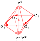
Figure 12: (Color online) The graphic representation of the phase factor $f_{3}(\alpha_{1},\alpha_{2},\alpha_{3},\alpha_{4},g,g^{*})$ in eqn. (30). The arrows on the edges that never form a oriented loop on any triangle represent the branching structure on the complex. The four tetrahedrons give rise to $\nu_{3}(\alpha_{1},\alpha_{2},g^{-1}g^{*},g^{*})$, $\nu_{3}(\alpha_{2},\alpha_{3},g^{-1}g^{*},g^{*})$, $\nu_{3}^{-1}(\alpha_{4},\alpha_{3},g^{-1}g^{*},g^{*})$, and $\nu_{3}^{-1}(\alpha_{1},\alpha_{4},g^{-1}g^{*},g^{*})$

The above discussion and result can be generalized to higher dimensions. Here we will discuss 2D SPT state as an example. We choose the 2D SPT state to be a “plaquette state” (see Fig. 8)

$$|\Psi_{\text{pSRE}}\rangle =\otimes_{\text{squares}}(\sum_{g\in G}|\alpha_{1}=g,\beta_{2}=g,\gamma_{3}=g,\lambda_{4}=g\rangle)$$ (29)

where we have assumed that physical states on each dot in Fig. 8 are labeled by the elements of the symmetry group $G$: $\alpha_{i},\beta_{i},...\in G$. The four dots in a linked square in Fig. 8 form a maximally entangled state $\sum_{g\in G}|\alpha_{1}=g,\beta_{2}=g,\gamma_{3}=g,\lambda_{4}=g\rangle$. We require that the state $|\Psi_{\text{pSRE}}\rangle$ is invariant under an on-site symmetry transformation (12) (where the four dots in each shaded square represent a site).

To construct an on-site symmetry transformation (12), in 2 dimensions, the action of $U^{\bm{i}}$ is chosen to be

$$\ \ \ \ U^{\bm{i}}(g)|\alpha_{1},\alpha_{2},\alpha_{3},\alpha_{4}\rangle$$ (30)

$$=f_{3}(\alpha_{1},\alpha_{2},\alpha_{3},\alpha_{4},g,g^{*})|g\alpha_{1},g\alpha_{2},g\alpha_{3},g\alpha_{4}\rangle.$$

Here $f_{3}(\alpha_{1},\alpha_{2},\alpha_{3},\alpha_{4},g,g^{*})$ is a phase factor that corresponds to the value of a 3-cocycle $\nu_{3}\in{\cal H}^{3}[G,U_{T}(1)]$ evaluated on the complex with a branching structure in Fig. 12:

$$\ \ \ \ f_{3}(\alpha_{1},\alpha_{2},\alpha_{3},\alpha_{4},g,g^{*})$$

$$=\frac{\nu_{3}(\alpha_{1},\alpha_{2},g^{-1}g^{*},g^{*})\nu_{3}(\alpha_{2},\alpha_{3},g^{-1}g^{*},g^{*})}{\nu_{3}(\alpha_{4},\alpha_{3},g^{-1}g^{*},g^{*})\nu_{3}(\alpha_{1},\alpha_{4},g^{-1}g^{*},g^{*})}.$$ (31)

In appendix G, we will show that $U^{\bm{i}}(g)$ defined above is indeed a linear representation of $G$ that satisfies eqn. (12). We will also show that (see appendix I and LABEL:CLW1152) in a basis where the many-body ground state is a simple product state, although $\otimes_{\bm{i}}U^{\bm{i}}(g)$ is an on-site symmetry transformation when acting on the bulk state, it cannot be an on-site symmetry transformation when viewed as a symmetry transformation acting on the effective low energy degrees of freedom on the boundary when the 3-cocycle $\nu_{3}$ is non-trivial.

VII SPT phases and topological non-linear $\sigma$-models

VII.1 The fixed-point action that does not depend on the space-time metrics

In the above, we have constructed SPT states and their symmetry transformations using the cocycles of the symmetry group. We can easily find the Hamiltonians such that the constructed SPT states are the exact ground states. In the following, we are going to discuss a Lagrangian formulation of the construction. We will systematically construct models in $d+1$ space-time dimensions that contain SPT orders characterized by elements in ${\cal H}^{1+d}[G,U_{T}(1)]$. It turns out that the Lagrangian formulation is simpler than the Hamiltonian formulation.

A SPT phase can be described by a non-linear $\sigma$-model of a field $\bm{n}(\bm{x},\tau)$, whose imaginary-time path integral is given by

$$Z=\int D\bm{n}\ \hskip 1.0pt\mathrm{e}^{-\int\hskip 1.0pt\mathrm{d}^{d}\bm{x}\hskip 1.0pt\mathrm{d}\tau\;{\cal L}[\bm{n}(\bm{x},\tau)]}.$$ (32)

We will call the term $\hskip 1.0pt\mathrm{e}^{-\int\hskip 1.0pt\mathrm{d}^{d}\bm{x}\hskip 1.0pt\mathrm{d}\tau\;{\cal L}[\bm{n}(\bm{x},\tau)]}$ the action-amplitude. The imaginary-time evolution operator from $\tau_{1}$ to $\tau_{2}$, $U[\bm{n}_{2}(\bm{x}),\bm{n}_{1}(\bm{x}),\tau_{2},\tau_{1}]$, can also be expressed as a path integral

$$U[\bm{n}_{2}(\bm{x}),\bm{n}_{1}(\bm{x}),\tau_{2},\tau_{1}]=\int D\bm{n}\ \hskip 1.0pt\mathrm{e}^{-\int\hskip 1.0pt\mathrm{d}^{d}\bm{x}\int_{\tau_{1}}^{\tau_{2}}\hskip 1.0pt\mathrm{d}\tau\;{\cal L}[\bm{n}(\bm{x},\tau)]}$$ (33)

with the boundary condition $\bm{n}(\bm{x},\tau_{1})=\bm{n}_{1}(\bm{x})$ and $\bm{n}(\bm{x},\tau_{2})=\bm{n}_{2}(\bm{x})$.

If the model has a symmetry, the field $\bm{n}$ transforms as $\bm{n}\to g\cdot\bm{n}$ under the symmetry transformation $g\in G$. The action-amplitude has the $G$ symmetry

$$\hskip 1.0pt\mathrm{e}^{-\int\hskip 1.0pt\mathrm{d}^{d}\bm{x}\hskip 1.0pt\mathrm{d}\tau\;{\cal L}[\bm{n}(\bm{x},\tau)]}=\hskip 1.0pt\mathrm{e}^{-\int\hskip 1.0pt\mathrm{d}^{d}\bm{x}\hskip 1.0pt\mathrm{d}\tau\;{\cal L}[g\cdot\bm{n}(\bm{x},\tau)]}.$$ (34)

To understand the low energy physics, we concentrate on the “orbit” generated by $G$ from a fixed $\bm{n}_{0}$: $\{g\cdot\bm{n}_{0};g\in G\}$. Such an “orbit” is a symmetric space $G/H$ where $H$ is the subgroup of $G$ that keeps $\bm{n}_{0}$ invariant: $H=\{h;h\cdot\bm{n}_{0}=\bm{n}_{0},h\in G\}$. We can always add degrees of freedom to expand the symmetric space $G/H$ to the maximal symmetric space, which is the whole space of the group $G$. So to study SPT phase, we can always start with a non-linear $\sigma$-model whose field takes value in the symmetry group $G$, the maximal symmetric space. Such a non-linear $\sigma$-model is described by a path integral

$$Z=\int Dg\ \hskip 1.0pt\mathrm{e}^{-\int\hskip 1.0pt\mathrm{d}^{d}\bm{x}\hskip 1.0pt\mathrm{d}\tau\;{\cal L}[g(\bm{x},\tau)]},\ \ \ \ g\in G.$$ (35)

We would like to consider non-linear $\sigma$-models that describe a SRE phase with finite energy gap and finite correlations. So a low energy fixed point action-amplitude $\hskip 1.0pt\mathrm{e}^{-\int\hskip 1.0pt\mathrm{d}^{d}\bm{x}\hskip 1.0pt\mathrm{d}\tau\;{\cal L}[g(\bm{x},\tau)]}$ must not depend on the space-time metrics. In other words, the fixed-point non-linear $\sigma$-model must be a topological quantum field theory.W8951 We will call such non-linear $\sigma$-model a topological non-linear $\sigma$-model. A trivial topological non-linear $\sigma$-model is given by the following fixed-point Lagrangian ${\cal L}_{\text{fix}}[g(\bm{x},\tau)]=0$ which describes the trivial SPT phase.

A non-trivial topological non-linear $\sigma$-model has a non-zero Lagrangian ${\cal L}_{\text{fix}}[g(\bm{x},t)]\neq 0$. However, the corresponding fixed-point action-amplitude $\hskip 1.0pt\mathrm{e}^{-\int\hskip 1.0pt\mathrm{d}^{d}\bm{x}\hskip 1.0pt\mathrm{d}\tau\;{\cal L}[g(\bm{x},\tau)]}$ does not depend on the space-time metrics. One possible form of the fixed-point Lagrangian ${\cal L}_{\text{fix}}[g(\bm{x},\tau)]$ is given by a pure topological $\theta$-term. As stated in section XI, the origin of the topological $\theta$-term may be the Berry phase in coherent state path integral. For a continuous non-linear $\sigma$-model whose field takes values in a continuous group $G$, the topological $\theta$-term is described by the action-amplitude $\hskip 1.0pt\mathrm{e}^{\int\hskip 1.0pt\mathrm{d}^{d}\bm{x}\hskip 1.0pt\mathrm{d}\tau\;{\cal L}_{\text{topo}}[g(\bm{x},\tau)]}$ that only depends on the mapping class from the space-time manifold $M$ to the group manifold $G$. Such kind of topological term is given by a closed $(1+d)$-form $\omega_{1+d}$ on the group manifold $G$ which is classified by $H^{1+d}(G,\mathbb{R})$. The corresponding action is given by $\int\hskip 1.0pt\mathrm{d}^{d}\bm{x}\hskip 1.0pt\mathrm{d}\tau\;{\cal L}_{\text{topo}}[g(\bm{x},\tau)]=\int\omega_{1+d}$.

The other possible form of the fixed-point Lagrangian ${\cal L}_{\text{fix}}[g(\bm{x},\tau)]$ is given by a WZW term.WZ7195 ; W8322 The WZW term is described by the action $S_{\text{WZW}}$ that cannot be expressed as a local integral on the space-time manifold $M$. That is to say, we cannot express $S_{\text{WZW}}$ as $S_{\text{WZW}}=\int\hskip 1.0pt\mathrm{d}^{d}\bm{x}\hskip 1.0pt\mathrm{d}\tau\;{\cal L}_{\text{WZW}}[g(\bm{x},\tau)]$. We have to view the space-time manifold $M$ as a boundary of another manifold $M_{\text{ext}}$ in one higher dimensions, $M=\partial M_{\text{ext}}$, and extend the field on $M$ to a field on $M_{\text{ext}}$. Then the WZW term $S_{\text{WZW}}$ can be expressed as a local integral on the extended manifold $M_{\text{ext}}$:

$$S_{\text{WZW}}=\int_{M_{\text{ext}}}\hskip 1.0pt\mathrm{d}^{1+d}\bm{x}\hskip 1.0pt\mathrm{d}\tau\;{\cal L}_{\text{WZW}}[g(\bm{x},\tau)]$$ (36)

such that $S_{\text{WZW}}$ mod $2\pi\hskip 1.0pt\mathrm{i}\hskip 1.0pt$ does not depend on how we extend $M$ to $M_{\text{ext}}$. A WZW term is given by a quantized closed $(d+2)$-form $\omega_{d+2}$ on the group manifold $G$:

$$S_{\text{WZW}}=\int_{M_{\text{ext}}}\omega_{d+2},$$ (37)

which clearly does not depend on the space-time metrics. Later, we will show that WZW terms in $(d+1)$-dimension space-time and for group $G$ are classified by the elements in ${\cal H}^{d+2}[G,U_{T}(1)]$.

We see that both the topological $\theta$-term and the WZW term do not depend on the space-time metrics. So the fixed-point Lagrangian may be given by a pure topological $\theta$-term and/or a pure WZW term.

VII.2 Lattice non-linear $\sigma$-model

We would like to stress that the topological $\theta$-term and the WZW term discussed above require both continuous group manifold and continuous space-time manifold.

On the other hand, in this paper, we are considering quantum disordered states that do not break any symmetry. So the field $g(\bm{x},\tau)$ fluctuates strongly at all length scale. The low energy effective theory has no smooth limit. Therefore, the low energy effective theory must be one defined on discrete space-time.

For discrete space-time, we no longer have non-trivial mapping class from space-time to the group $G$, and we no longer have topological $\theta$-term and WZW term. In this section we will show that although a generic topological $\theta$-term cannot be defined for discrete space-time, we can construct a new topological term on discrete space-time that corresponds to a quantized topological $\theta$-term in the limit of continuous space-time. Here a quantized topological $\theta$-term is defined as a topological $\theta$-term that always gives rise to an action-amplitude $\hskip 1.0pt\mathrm{e}^{\int\hskip 1.0pt\mathrm{d}^{d}\bm{x}\hskip 1.0pt\mathrm{d}\tau\;{\cal L}_{\text{fix}}[g(\bm{x},\tau)]}=1$ on closed space-time. We will also call the new topological term on discrete space-time a quantized topological $\theta$-term.

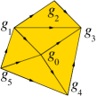
Figure 13: (Color online) The graphic representation of the action-amplitude $\hskip 1.0pt\mathrm{e}^{-S(\{g_{i}\})}$ on a complex with a branching structure represented by the arrows on the edge. The vertices of the complex are labeled by $i$. Note that the arrows never for a loop on any triangle.

To understand the new topological term on discrete space-time, let us start with a continuous non-linear $\sigma$-model whose field takes values in a group $G$: $g(\bm{x},t)$. The imaginary-time path integral of the model is given by

$$Z=\int Dg\ \hskip 1.0pt\mathrm{e}^{-\int\hskip 1.0pt\mathrm{d}^{d}\bm{x}\hskip 1.0pt\mathrm{d}\tau\;{\cal L}[g(\bm{x},\tau)]}$$ (38)

with a symmetry described by $G$:

$$\hskip 1.0pt\mathrm{e}^{-\int\hskip 1.0pt\mathrm{d}^{d}\bm{x}\hskip 1.0pt\mathrm{d}\tau\;{\cal L}[g(\bm{x},\tau)]}=\hskip 1.0pt\mathrm{e}^{-\int\hskip 1.0pt\mathrm{d}^{d}\bm{x}\hskip 1.0pt\mathrm{d}\tau\;{\cal L}[gg(\bm{x},\tau)]},\ \ \ \ g\in G.$$ (39)

If we discretize the space-time into a complex with a branching structure (such as the complex obtained by a triangularization of the space-time manifold), the path integral can be rewritten as (see Fig. 13)

$$Z =|G|^{-N_{v}}\sum_{\{g_{i}\}}\hskip 1.0pt\mathrm{e}^{-S(\{g_{i}\})}$$

$$\hskip 1.0pt\mathrm{e}^{-S(\{g_{i}\})} =\prod_{\{ij...k\}}\nu_{1+d}^{s_{ij...k}}(g_{i},g_{j},...,g_{k})$$ (40)

where $\hskip 1.0pt\mathrm{e}^{-S(\{g_{i}\})}$ is the action-amplitude on the discretized space-time that corresponds to $\hskip 1.0pt\mathrm{e}^{-\int\hskip 1.0pt\mathrm{d}^{d}\bm{x}\hskip 1.0pt\mathrm{d}\tau\;{\cal L}[g(\bm{x},\tau)]}$ of the continuous non-linear $\sigma$-model, and $\nu_{1+d}^{s_{ij...k}}(g_{i},g_{j},...,g_{k})$ corresponds to the action-amplitude $\hskip 1.0pt\mathrm{e}^{-\int_{(i,j,...,k)}\hskip 1.0pt\mathrm{d}^{d}\bm{x}\hskip 1.0pt\mathrm{d}\tau\;{\cal L}[g(\bm{x},\tau)]}$ on a single simplex $(i,j,...,k)$. Also, $s_{ij...k}=\pm 1$ depending on the orientation of the simplex (which will be explained in detail later).

Here on each vertex of the space-time complex, we have a $g_{i}\in G$. $g_{i}$ corresponds to the field $g(\bm{x},t)$ and $\sum_{\{g_{i}\}}$ corresponds to the path integral $\int Dg$ in the continuous non-linear $\sigma$-model. $|G|$ is the number of elements in $G$, $N_{v}$ is the number of vertices in the complex.

We note that, on discrete space-time, the model can be defined for both continuous group and discrete group. When $G$ is a continuous group, $|G|^{-1}\sum_{g_{i}}$ should be interpreted as an integral over the group manifold $\int\hskip 1.0pt\mathrm{d}g_{i}$.

We see that a non-linear $\sigma$-model on $(d+1)$D discrete space-time is described by a complex function $\nu_{1+d}(g_{i},g_{j},...,g_{k})$. Different choices of $\nu_{1+d}(g_{i},g_{j},...,g_{k})$ give different theories/models.

So we would like to ask: what $\nu_{1+d}(g_{i},g_{j},...,g_{k})$ will give rise to a quantized topological $\theta$-term on discrete space-time? Very simply, we need to choose $\nu_{1+d}(g_{i},g_{j},...,g_{k})$ so that

$$\prod_{\{ij...k\}}\nu_{1+d}^{s_{ij...k}}(g_{i},g_{j},...,g_{k})=1$$ (41)

on every closed space-time complex without boundary.

There are uncountably many choices of $\nu_{1+d}(g_{i},g_{j},...,g_{k})$ that satisfy the above condition and give rise to quantized topological $\theta$-terms. However, we can group them into equivalent classes, and each class corresponds to a type of quantized topological $\theta$-terms. We will show later that the types of quantized topological $\theta$-terms are classified by ${\cal H}^{1+d}[G,U_{T}(1)]$. So we can have non-trivial quantized topological $\theta$-terms discrete space-time only when ${\cal H}^{1+d}[G,U_{T}(1)]$ is non trivial. The number of equivalence classes of non-trivial quantized topological $\theta$-terms is given by the number of the non-trivial elements in ${\cal H}^{1+d}[G,U_{T}(1)]$.

From the above discussion, it is also clear that we cannot generalize un-quantized topological $\theta$-terms to discrete space-time. So on discretized space-time complex, the only possible topological $\theta$-terms are the quantized ones.

After generalizing quantized topological $\theta$-terms to discrete space-time, we can now generalize WZW term to discrete space-time. We will call the generalized WZW term a non-local Lagrangian (NLL) term. To construct a NLL term on a closed $(d+1)$D space-time complex $M_{d+1}$, we first view $M_{d+1}$ as a boundary of a $(d+2)$D space-time complex $M_{d+2}$. We then choose a function $\nu_{2+d}(g_{i},g_{j},...,g_{k})$ that defines a quantized topological $\theta$-term on the $(d+2)$D space-time complex $M_{d+2}$. Then the action-amplitude of $\nu_{2+d}(g_{i},g_{j},...,g_{k})$ on $M_{d+2}$ only depends on the $g_{i}$ on $M_{d+1}=\partial M_{d+2}$, the boundary of $M_{d+2}$. Thus such an action-amplitude actually defines a theory on the $(d+1)$D space-time complex $M_{d+1}$. Such an action-amplitude is the NLL term on the space-time complex $M_{d+1}$. We will see that the types of NLL terms on $(d+1)$D space-time complex and for group $G$ are classified by ${\cal H}^{2+d}[G,U_{T}(1)]$.

We would like to stress that the proper topological non-linear $\sigma$-models are for disordered phases, and they must be defined on discrete space-time. Only quantized topological $\theta$-terms can be defined on discrete space-time. On the other hand, the WZW term can always be generalized to discrete space-time, which is called NLL term. Both quantized topological $\theta$-terms and NLL terms on discrete space-time can be defined for discrete groups.

VII.3 Quantized topological $\theta$-terms lead to gapped SPT phases

We know that the action-amplitude defines a physical model, in particular, defines imaginary-time evolution operator $U(\tau_{1},\tau_{2})$. For a SPT phase, its fixed point action-amplitude must have the following properties (on a closed spatial complex):
(a) The singular values of the imaginary-time evolution operator $U[g_{i}(\tau_{1}),g_{i}(\tau_{2}),\tau_{1},\tau_{2}]$ are 1’s or 0’s.
(b) The singular values of the imaginary-time evolution operator $U[g_{i}(\tau_{1}),g_{i}(\tau_{2}),\tau_{1},\tau_{2}]$ contain only one 1.

Usually, the imaginary-time evolution operator is given by $U(\tau_{1},\tau_{2})=\hskip 1.0pt\mathrm{e}^{-(\tau_{2}-\tau_{1})H}$. One expects that the log of the eigenvalues of $U(\tau_{1},\tau_{2})$ correspond to the negative energies. However, in general, the basis of the Hilbert space at different time $\tau$ can be chosen to be different. Such a time dependent choice of the basis corresponds to adding a total time derivative term to the Lagrangian ${\cal L}\to{\cal L}+\frac{\hskip 1.0pt\mathrm{d}F}{\hskip 1.0pt\mathrm{d}\tau}$. It is well known that adding a total time derivative term to the Lagrangian does not change any physical properties. For such more general cases, the log of the eigenvalues of $U(\tau_{1},\tau_{2})$ do not correspond to the negative energies, since the eigenvalues of $U(\tau_{1},\tau_{2})$ may be complex numbers. In those cases, the log of the singular values of $U(\tau_{1},\tau_{2})$ correspond to the negative energies. This is why we use the singular values of $U(\tau_{1},\tau_{2})$ instead of the eigenvalues of $U(\tau_{1},\tau_{2})$.

At the low energy fixed point of a gapped system, the fixed-point energies are either 0 or infinite. Thus the singular values of the imaginary-time evolution operator are either 1 or 0. For a SPT phase without any intrinsic topological order and without any symmetry breaking, the ground state degeneracy on a closed spatial complex is always one. Thus the singular values of the imaginary-time evolution operator contain only one 1.

For the action-amplitude given by a quantized topological $\theta$-term, its corresponding imaginary-time evolution operator does have a property that its singular values contain only one 1 and the rest are 0’s. This is due to the fact that the action-amplitude for each closed path is always equal to 1. So a quantized topological $\theta$-term indeed describes a SPT state.

VII.4 NLL terms lead to gapless excitations or degenerate boundary states

On the other hand, if the fixed-point action-amplitude in $(d+1)$ space-time dimension is given by a pure NLL term, its corresponding imaginary-time evolution operator, we believe, does not have the property that its singular values contain only one 1 and the rest are 0’s, since the action-amplitude for different closed paths can be different.

In addition, if the pure NLL term corresponds to a non-trivial cocycle $\nu_{d+2}$ in ${\cal H}^{d+2}[G,U_{T}(1)]$, adding different coboundary to $\nu_{d+2}$ will lead to different action-amplitude on closed paths. There is no coboundary that we can add to the cocycle $\nu_{d+2}$ to make the action-amplitude for closed paths all equal to 1. Further more, a renormalization group flow only adds local Lagrangian term $\delta{\cal L}$ that is well defined on the space-time complex. The renormalization group flow cannot change the NLL term and cannot change the corresponding cocycle $\nu_{d+2}$, which is defined in one higher dimensions. This leads us to conclude that an action-amplitude with a NLL term cannot describe a SPT state. Therefore

An action-amplitude with a NLL term must have gapless excitations, or degenerate boundary ground states due to symmetry breaking and/or topological order.

The above is a highly non-trivial conjecture. Let us examine its validity for some simple cases. Consider a $G$ symmetric non-linear $\sigma$-model in (1+0) dimension which is described by an action-amplitude with a NLL term. In (1+0) dimension, the NLL term is classified by 2-cocycles $\nu_{2}$ in ${\cal H}^{2}[G,U_{T}(1)]$, which correspond to the projective representations of the symmetry group $G$. So the ground states of the non-linear $\sigma$-model form a projective representation of $G$ characterized by the same 2-cocycle $\nu_{2}$. Since projective representations are always more than one dimension, (1+0)D systems with NLL terms cannot have a non-degenerate ground state. In (1+1)-dimension, continuous non-linear $\sigma$-models with the WZW term are shown to be described by the current algebra of the continuous symmetry group and are gapless.W8322 In LABEL:CLW1152, we further show that lattice non-linear $\sigma$-models with the NLL term in (1+1)D must be gapless if the symmetry is not broken, for both continuous and discrete symmetry. The above conjecture generalize such a result to higher dimensions.

We note that the boundary excitations of the SPT phases characterized by $(1+d)$-cocycle $\nu_{1+d}$ are described by an effective boundary non-linear $\sigma$-model that contains a NLL term characterized by the same $(1+d)$-cocycle $\nu_{1+d}$.

As discussed before, a non-linear $\sigma$-model with a non-trivial NLL term cannot describe a SPT state. Thus the boundary state must be gapless, or break the symmetry, or have degeneracy due to non-trivial topological order. However, the SPT state is a direct product state. The degrees of freedom on the boundary also form a product state. Therefore the boundary state must be gapless, or break the symmetry. Thus,

A non-trivial SPT state described by a non-trivial $$(1+d)$$-cocycle must have gapless excitations or degenerate ground states at the boundary.

We would like to stress that the symmetry plays a very important role in the above discussion. It is the reason why the non-linear $\sigma$-model field $g_{i}$ takes many different values. If there was no symmetry, at low energies, the non-linear $\sigma$-model field $g_{i}$ would only take a single value that minimizes the local potential energy. In this case, there were no non-trivial topological terms.

VIII Constructing symmetric fixed-point path integral through the cocycles of the symmetry group

In the last section, we argue that SPT phases in $d$-dimension with on-site symmetry $G$ are described by quantized topological $\theta$-terms. In this section, we are going to explicitly construct quantized topological $\theta$-terms that realize those SPT orders in each space-time dimension. We will also show that the quantized topological $\theta$-terms are classified by ${\cal H}^{1+d}[G,U_{T}(1)]$.

VIII.1 (1+1)D symmetric fixed-point action-amplitude

Let us first discuss (1+1)D fixed-point action-amplitude with a symmetry group $G$. For a $(1+1)$D system on a complex with a branching structure, a fixed-point action-amplitude (ie a quantized topological $\theta$-term) has a form (see Fig. 13)

$$\ \ \ \ \hskip 1.0pt\mathrm{e}^{-S(\{g_{i}\})}=\prod_{\{ijk\}}\nu_{2}^{s_{ijk}}(g_{i},g_{j},g_{k})$$

$$=\nu_{2}^{-1}(g_{1},g_{2},g_{3})\nu_{2}(g_{0},g_{4},g_{3})\nu_{2}^{-1}(g_{5},g_{0},g_{1},)\times$$

$$\ \ \ \ \ \ \ \ \nu_{2}(g_{1},g_{0},g_{3})\nu_{2}^{-1}(g_{5},g_{0},g_{4})$$ (42)

where each triangle contributes to a phase factor $\nu_{2}^{s_{ijk}}(g_{i},g_{j},g_{k})$, $\prod_{\{ijk\}}$ multiply over all the triangles in the complex Fig. 13. Note that the first variable $g_{i}$ in $\nu_{2}(g_{i},g_{j},g_{k})$ corresponds to the vertex with two out going edges, the second variable $g_{j}$ to the vertex with one out going edge, and the third variable $g_{k}$ to the vertex with no out going edge. $s_{ijk}=\pm 1$ depending on the orientation of $i\to j\to k$ to be anti-clock-wise or clock-wise.

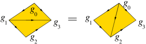
Figure 14: (Color online) Graphic representation of $\nu_{2}(g_{0},g_{1},g_{2})\nu_{2}(g_{0},g_{2},g_{3})=\nu_{2}(g_{1},g_{2},g_{3})\nu_{2}(g_{0},g_{1},g_{3})$ The arrows on the edges represent the branching structure.

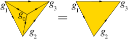
Figure 15: (Color online) Graphic representation of $\nu_{2}(g_{1},g_{2},g_{3})=\nu_{2}(g_{0},g_{1},g_{2})\nu_{2}(g_{0},g_{2},g_{3})\nu_{2}^{-1}(g_{0},g_{1},g_{3})$. The arrows on the edges represent the branching structure.

In order for the action-amplitude to represent a quantized topological $\theta$-term, we must choose $\nu_{2}(g_{i},g_{j},g_{k})$ such that

$$\hskip 1.0pt\mathrm{e}^{-S(\{g_{i}\})}=\prod_{\{ijk\}}\nu_{2}^{s_{ijk}}(g_{i},g_{j},g_{k})=1$$ (43)

on closed space-time complex without boundary, in particular, on a tetrahedron with four triangles (see Fig. 10):

$$\hskip 1.0pt\mathrm{e}^{-S(\{g_{i}\})} =\prod_{\{ijk\}}\nu_{2}^{s_{ijk}}(g_{i},g_{j},g_{k})$$

$$=\frac{\nu_{2}(g_{1},g_{2},g_{3})\nu_{2}(g_{0},g_{1},g_{3})}{\nu_{2}(g_{0},g_{1},g_{2})\nu_{2}(g_{0},g_{2},g_{3})}=1$$ (44)

Also, in order for our system to have the symmetry generated by the group $G$, its action-amplitude must satisfy

$$\hskip 1.0pt\mathrm{e}^{-S(\{g_{i}\})} =\hskip 1.0pt\mathrm{e}^{-S(\{gg_{i}\})},\text{ if }g\text{ contains no T}$$

$$\Big{(}\hskip 1.0pt\mathrm{e}^{-S(\{g_{i}\})}\Big{)}^{\dagger} =\hskip 1.0pt\mathrm{e}^{-S(\{gg_{i}\})},\text{ if }g\text{ contains one T}$$ (45)

where $T$ is the time-reversal transformation. This requires

$$\nu_{2}^{s(g)}(g_{i},g_{j},g_{k})=\nu_{2}(gg_{i},gg_{j},gg_{k}).$$ (46)

Eqn. (VIII.1) and eqn. (46) happen to be the conditions of 2-cocycles $\nu_{2}(g_{0},g_{1},g_{2})$ of $G$. Thus the action-amplitude eqn. (VIII.1) constructed from a 2-cocycle $\nu_{2}(g_{0},g_{1},g_{2})$ is a quantized topological $\theta$-term.

If $\nu_{2}(g_{0},g_{2},g_{3})$ satisfies eqn. (VIII.1) and eqn. (46), then

$$\nu_{2}^{\prime}(g_{0},g_{2},g_{3})=\nu_{2}(g_{0},g_{2},g_{3})\frac{\mu_{1}(g_{1},g_{2})\mu_{1}(g_{0},g_{1})}{\mu_{1}(g_{0},g_{2})}$$ (47)

also satisfies eqn. (VIII.1) and eqn. (46), for any $\mu_{1}(g_{0},g_{1})$ satisfying $\mu_{1}(gg_{0},gg_{1})=\mu_{1}(g_{0},g_{1})$, $g\in G$. So $\nu_{2}^{\prime}(g_{0},g_{2},g_{3})$ also gives rise to a quantized topological $\theta$-term. As we continuously deform $\mu_{1}(g_{0},g_{1})$, the two quantized topological $\theta$-terms can be smoothly connected. So we say that the two quantized topological $\theta$-terms obtained from $\nu_{2}(g_{0},g_{2},g_{3})$ and $\nu_{2}^{\prime}(g_{0},g_{2},g_{3})$ are equivalent. We note that $\nu_{2}(g_{0},g_{2},g_{3})$ and $\nu_{2}^{\prime}(g_{0},g_{2},g_{3})$ differ by a 2-coboundary $\frac{\mu_{1}(g_{1},g_{2})\mu_{1}(g_{0},g_{1})}{\mu_{1}(g_{0},g_{2})}$. So the set of equivalence classes of $\nu_{2}(g_{0},g_{2},g_{3})$ is nothing but the cohomology group ${\cal H}^{2}[G,U_{T}(1)]$. Therefore, the quantized topological $\theta$-terms are classified by ${\cal H}^{2}[G,U_{T}(1)]$.

We can also show that eqn. (VIII.1) is a fixed-point action-amplitude from the cocycle conditions on $\nu_{2}(g_{i},g_{j},g_{k})$. From the geometrical picture of the cocycles (see Fig. 10), we have the following relations: $\nu_{2}(g_{0},g_{1},g_{2})\nu_{2}(g_{0},g_{2},g_{3})=\nu_{2}(g_{1},g_{2},g_{3})\nu_{2}(g_{0},g_{1},g_{3})$ (see Fig. 14) and $\nu_{2}(g_{1},g_{2},g_{3})=\nu_{2}(g_{0},g_{1},g_{2})\nu_{2}(g_{0},g_{2},g_{3})\nu_{2}^{-1}(g_{0},g_{1},g_{3})$. (see Fig. 15). We can use those two basic moves to generate a renormalization flow that induces a coarse-grain transformation of the complex. The two relations Fig. 14 and Fig. 15 imply that the action-amplitude is invariant under the renormalization flow. So it is a fixed-point action-amplitude. Certainly, the above construction applies to any dimensions.

VIII.2 (1+1)D fixed-point ground state wave function

For our fixed-point theory described by a quantized topological $\theta$-term, its ground state wave function $\Psi(\{g_{i}\})$ can be obtained by putting $g_{i}$ on the edge of a disk and making a triangularization of the disk (see Fig. 13). We sum the action-amplitude over the $g_{i}$ on the internal vertices while fixing the $g_{i}$’s on the edge (see Fig. 16a):

$$\Psi(\{g_{i}\}_{\text{edge}}) =\frac{\sum_{g_{i}\in\text{internal}}}{|G|^{N^{\text{internal}}_{v}}}\prod_{\{ijk\}}\nu_{2}^{s_{ijk}}(g_{i},g_{j},g_{k})$$ (48)

where $\sum_{g_{i}\in\text{internal}}$ sums over $g_{i}$ on the internal vertices and $N^{\text{internal}}_{v}$ is the number of internal vertices on the disk.

Figure 16: (Color online) (a) The graphic representation of $\Psi(\{g_{i}\}_{\text{edge}})=\nu_{2}^{-1}(g_{1},g_{2},g_{3})\nu_{2}^{-1}(g_{1},g_{3},g_{5})\nu_{2}^{-1}(g_{3},g_{4},g_{5})$ (b) The graphic representation of $\Psi^{\dagger}(\{g_{i}\}_{\text{edge}})=\nu_{2}(g_{1},g_{2},g_{3})\nu_{2}(g_{1},g_{3},g_{5})\nu_{2}(g_{3},g_{4},g_{5})$ The arrows on the edges represent the branching structure.

Clearly the ideal wave function $\Psi(\{g_{i}\}_{\text{edge}})$ satisfies

$$\Psi^{s(g)}(\{g_{i}\}_{\text{edge}})=\Psi(\{gg_{i}\}_{\text{edge}}),\ \ \ \ |\Psi(\{g_{i}\}_{\text{edge}})|=1,$$ (49)

which represents a symmetric state. We also note that $\Psi^{\dagger}(\{g_{i}\}_{\text{edge}})$ can be represented by Fig. 16b, since the product of the wave functions in Fig. 16a and Fig. 16b is the value of the cocycle on a sphere which is equal to 1.

VIII.3 (2+1)D symmetric fixed-point action-amplitude

In $(2+1)$D, our ideal model with on-site symmetry $G$ is defined by the action-amplitude on a 3D complex with $g_{i}\in G$ on each vertex:

$$\hskip 1.0pt\mathrm{e}^{-S(\{g_{i}\})}=\prod_{\{ijkl\}}\nu_{3}^{s_{ijkl}}(g_{i},g_{j},g_{k},g_{l})$$ (50)

where $\nu_{3}(g_{i},g_{j},g_{k},g_{l})$ is a three cocycle and $\prod_{\{ijkl\}}$ multiply over all the tetrahedrons in the complex Fig. 17. The 3D complex has a branching structure. The first variable $g_{i}$ is on the vertex with no incoming edge, the second variable $g_{j}$ is on the vertex with one incoming edge, etc . Also $s_{ijkl}=\pm 1$ depending on the orientation of the $ijkl$-tetrahedron. On a close space-time complex, the above action-amplitude is always equal to 1 due to the cocycle condition on $\nu_{3}(g_{i},g_{j},g_{k},g_{l})$. Thus the above action-amplitude is a quantized topological $\theta$-term.

Figure 17: Two solid tetrahedrons $g_{0}g_{1}g_{2}g_{4}$, $g_{0}g_{2}g_{3}g_{4}$ and three solid tetrahedrons $g_{0}g_{1}g_{2}g_{3}$, $g_{0}g_{1}g_{3}g_{4}$, $g_{1}g_{2}g_{3}g_{4}$ occupy the same volume, which leads to the graphic representation of $\nu_{3}(g_{0},g_{1},g_{2},g_{4})\nu_{3}(g_{0},g_{2},g_{3},g_{4})=\nu_{3}(g_{0},g_{1},g_{2},g_{3})\nu_{3}(g_{0},g_{1},g_{3},g_{4})\nu_{3}(g_{1},g_{2},g_{3},g_{4})$ (see eqn. (20)). The arrows on the edges represent the branching structure.

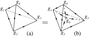
Figure 18: One solid tetrahedron $g_{1}g_{2}g_{3}g_{4}$, and four solid tetrahedrons $g_{0}g_{1}g_{2}g_{4}$, $g_{0}g_{2}g_{3}g_{4}$, $g_{0}g_{1}g_{3}g_{4}$, $g_{1}g_{1}g_{2}g_{3}$ occupy the same volume, which leads to the graphic representation of $\nu_{3}(g_{1},g_{2},g_{3},g_{4})=\nu_{3}(g_{0},g_{1},g_{2},g_{4})\nu_{3}(g_{0},g_{2},g_{3},g_{4})\nu_{3}^{-1}(g_{0},g_{1},g_{3},g_{4})\nu_{3}^{-1}(g_{0},g_{1},g_{2},g_{3})$ (see eqn. (20)). The arrows on the edges represent the branching structure.

The conditions of 3-cocycle lead to the two relations in Fig. 17 and Fig. 18. These lead to a renormalization flow of the complex in which the above action-amplitude is a fixed-point action-amplitude. The fixed-point action-amplitude leads to an ideal short-range-entangled state (see section IX) that has a symmetry $G$ and is characterized by $\nu_{3}\in{\cal H}^{3}[G,U_{T}(1)]$.

VIII.4 $(d+1)$D symmetric fixed-point action-amplitude

Through the above two examples in (1+1)D and (2+1)D, we see that the $(d+1)$D symmetric fixed-point action-amplitude is given by

$$Z =\frac{\sum_{\{g_{i}\}}}{|G|^{N_{v}}}\prod_{\{ij...k\}}\nu_{1+d}^{s_{ij...k}}(g_{i},g_{j},...,g_{k})$$ (51)

where $g_{i}$ is associated with each vertex on the space-time complex and $N_{v}$ is the number of vertices. $\sum_{\{g_{i}\}}$ sums over all possible configurations of $\{g_{i}\}$ and $\nu_{1+d}(g_{i},g_{j},...,g_{k})$ is a $(1+d)$-cocycle in ${\cal H}^{1+d}[G,U_{T}(1)]$.

When the space-time complex is closed (ie has no boundary), the action-amplitude $\prod_{\{ij...k\}}\nu_{1+d}^{s_{ij...k}}(g_{i},g_{j},...,g_{k})$ is always equal to 1. Thus the action-amplitude represents a topological $\theta$-term.

When the space-time complex has a boundary, the action-amplitude will not always be equal to 1 and is not trivial. We note that, due to the cocycle condition on $\nu_{1+d}^{s_{ij...k}}(g_{i},g_{j},...,g_{k})$, such a action-amplitude will only depend on $g_{i}$’s on the boundary of the space-time complex. Thus such an action-amplitude can be viewed as an action-amplitude of the boundary theory.

As an action-amplitude of the boundary theory, $\prod_{\{ij...k\}}\nu_{1+d}^{s_{ij...k}}(g_{i},g_{j},...,g_{k})$ is actually a NLL term, which is a generalization of the WZW topological term for continuous non-linear $\sigma$-models to lattice non-linear $\sigma$-models. So the boundary excitations of our model defined by eqn. (51) are described by a non-linear $\sigma$-model with a NLL term composed by the same $\nu_{1+d}\in{\cal H}^{1+d}[G,U_{T}(1)]$. We see a close relation between the topological $\theta$-term in $(d+1)$ space-time dimensions and the NLL term in $d$ space-time dimensions. An example of such a relation has been discussed by Ng for a (1+1)D model with $SO(3)$ symmetry.N9455 When $\nu_{1+d}$ is non-trivial, we believe that the boundary states are gapless or degenerate on the boundary.

In the following, we will show that the ground state wave function of our model (51) describes a SPT state.

IX Trivial intrinsic topological order in our fixed-point models

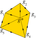
Figure 19: (Color online) The graphic representation of eqn. (52). The boundary is the complex $M$, and the whole complex $M_{\text{ext}}$ is an extension of $M$.

The ground state of our $d$-dimensional model (51) is a wave function $\Psi_{M}$ on $M$, a $d$-dimensional complex. It is given by (see Fig. 19)

$$\Psi_{M}(\{g_{i}\}_{M}) =\frac{\sum_{g_{i}\in\text{internal}}}{|G|^{N^{\text{internal}}_{v}}}\prod_{\{ij...k\}}\nu_{1+d}^{s_{ij...k}}(g_{i},g_{j},...,g_{k})$$ (52)

which generalizes eqn. (48) from (1+1)-D to $(d+1)$-D. We use $M_{\text{ext}}$ to denote a $(d+1)$ dimensional complex whose boundary is $M$. $\{g_{i}\}_{M}$ are on the vertices on $M$ and $\sum_{g_{i}\in\text{internal}}$ sums over the $g_{i}$’s on the vertices inside the complex $M_{\text{ext}}$ (not on its boundary $M$). Also $\prod_{\{ij...k\}}$ is product over all simplices on $M_{\text{ext}}$.

Due to the cocycle condition satisfied by $\nu_{1+d}(g_{i},g_{j},...,g_{k})$, we see that, for fixed $\{g_{i}\}_{M}$, the product $\prod_{\{ij...k\}}\nu_{1+d}^{s_{ij...k}}(g_{i},g_{j},...,g_{k})$ does not depend on $g_{i}$’s on the vertices inside the complex $M_{\text{ext}}$. Thus

$$\Psi_{M}(\{g_{i}\}_{M}) =\prod_{\{ij...*\}}\nu_{1+d}^{s_{ij...*}}(g_{i},g_{j},...,g^{*}).$$ (53)

if we choose $M_{\text{ext}}$ to be $M$ plus one more vertex with label $g^{*}$ (see Fig. 19). The state on $M$ (the boundary of Fig. 19) does not depend on the choice of $g^{*}$.

Using the above expression, we can show that the ground state wave function of our fixed-point model is SRE state with no intrinsic topological orders. Let us first write the ground state of our fixed-point model in a form

$$|\Psi_{M}\rangle =\sum_{\{g_{i}\}_{M}}\prod_{\{ij...*\}}\nu_{1+d}^{s_{ij...*}}(g_{i},g_{j},...,g^{*})|\{g_{i}\}_{M}\rangle,$$ (54)

where $|\{g_{i}\}_{M}\rangle$ form a basis of our model on $d$-dimensional complex $M$. The on-site symmetry acts in a simple way:

$$g:\ |\{g_{i}\}_{M}\rangle\to|\{gg_{i}\}_{M}\rangle,\ g\in G$$ (55)

We note that if we choose the particular form of $M_{\text{ext}}$ in Fig. 19 to obtain state $\Phi_{M}$ on $M$, the phase factor $\prod_{\{ij...*\}}\nu_{1+d}^{s_{ij...*}}(g_{i},g_{j},...,g^{*})$ can be viewed as a LU transformation. We can write $|\Psi_{M}\rangle$ in a new basis $|\{g_{i}\}_{M}\rangle^{\prime}=\prod_{\{ij...*\}}\nu_{1+d}^{s_{ij...*}}(g_{i},g_{j},...,g^{*})|\{g_{i}\}_{M}\rangle$:

$$|\Psi_{M}\rangle =\sum_{\{g_{i}\}_{M}}|\{g_{i}\}_{M}\rangle^{\prime}.$$ (56)

Thus, on any complex $M$ that can be viewed as a boundary of another complex $M_{\text{ext}}$, the state on $M$ can be transformed by an LU transformation into a state that is the equal weight superposition of all possible states $|\{g_{i}\}_{M}\rangle$ on $M$. The wave function in the new bases is very simple, which is actually a product state. In appendix H, we will show that under a dual transformation, this product state is equivalent to the canonical form of wave function discussed in Sec. IV and V.

We have used the $(1+d)$-cocycles in ${\cal H}^{1+d}[G,U_{T}(1)]$ to construct our fixed-point models which have ground state wave functions that also depend on the $(1+d)$-cocycles. In the above, we have shown that all those states can be mapped to the same simple product state via LU transformations. Does this mean that those states from different $(1+d)$-cocycles all belong to the same phase? The answer depends on if symmetry is included or not.

If we do not include any symmetry, those states from different $(1+d)$-cocycles indeed all belong to the same trivial phase. Thus our fixed-point states constructed from different $(1+d)$-cocycles all have trivial intrinsic topological order. This is consistent with the fact that the fixed-point partition function on any space-time complex has the form

$$Z=e^{-S_{0}V},$$ (57)

where $V$ is the volume of the space-time complex (say $V$ is the number of simplices in the space-time complex). We would like to stress that the above expression is exact. So after we remove the term that is proportional to the space-time volume, we have $Z=1$. This means that the ground state is not degenerate on any closed space complex, which in turn implies that the ground state contains no intrinsic topological order.

On the other hand, if we include the on-site symmetry $G$, states from different $(1+d)$-cocycles belong to the different phases which correspond to different SPT phases. This is because the LU transformation represented by $\prod_{\{ij...*\}}\nu_{1+d}^{s_{ij...*}}(g_{i},g_{j},...,g^{*})$ is not a symmetric LU transformation under the on-site symmetry $G$. To see this, we first note that the LU transformation $\prod_{\{ij...*\}}\nu_{1+d}^{s_{ij...*}}(g_{i},g_{j},...,g^{*})$ contains several layers of non-overlapping terms. For example, for the (1+1)D system in Fig. 19, the LU transformation has two layers

$$\prod_{\{ijk\}}\nu_{2}(g_{i},g_{j},g_{k})=[\nu_{2}(g_{3},g_{2},g^{*})\nu_{2}(g_{5},g_{4},g^{*})]\times$$

$$\ \ \ \ \ \ \ \ \ \ \ \ [\nu_{2}(g_{2},g_{1},g^{*})\nu_{2}(g_{4},g_{3},g^{*})\nu_{2}(g_{1},g_{5},g^{*})]$$ (58)

In order for the LU transformation to be a symmetric, each local term, such as $\nu_{2}(g_{2},g_{1},g^{*})$, must transform as

$$\nu_{2}^{s(g)}(g_{2},g_{1},g^{*})=\nu_{2}(gg_{2},gg_{1},g^{*})$$ (59)

under the on-site symmetry transformation generated by $g\in G$: Although $\nu_{2}^{s(g)}(g_{2},g_{1},g^{*})=\nu_{2}(gg_{2},gg_{1},gg^{*})$, in general $\nu_{2}^{s(g)}(g_{2},g_{1},g^{*})\neq\nu_{2}(gg_{2},gg_{1},g^{*})$. In fact, only trivial cocycle in ${\cal H}^{1+d}[G,U_{T}(1)]$ can satisfy $\nu_{1+d}^{s(g)}(g_{1},g_{2},..,g_{1+d},g^{*})=\nu_{1+d}(gg_{1},gg_{2},..,gg_{1+d},g^{*})$. Thus the fixed-point states from different $(1+d)$-cocycles belong to the different SPT phases.

We have seen that we can use two different basis $|\{g_{i}\}_{M}\rangle$ and $|\{g_{i}\}_{M}\rangle^{\prime}$ to expand the fixed-point wave function $|\Psi_{M}\rangle$. The old basis $|\{g_{i}\}_{M}\rangle$ transforms simply under the symmetry transformation: $|\{g_{i}\}_{M}\rangle\to|\{gg_{i}\}_{M}\rangle$. But the wave function $\Psi_{M}(\{g_{i}\})$ in the old basis is complicated. In the new basis, the wave function is very simple $\Psi^{\prime}_{M}(\{g_{i}\})=1$. But the symmetry transformation is more complicated in the new basis which will be discussed in appendix H.

In section VI, we discuss the SPT phase by starting with a simple many-body wave function, and try to classify all the allowed on-site symmetry transformations. Such a formalism is closely related to the new basis.

X Equivalent cocycles give rise to the same SPT phase

The ground state wave function $\Psi_{M}(\{g_{i}\}_{M})$ of a SPT phase is constructed from a cocycle $\nu_{1+d}$ as in eqn. (53). Let $\nu^{\prime}_{1+d}$ be a cocycle that is equivalent to $\nu_{1+d}$. That is $\nu_{1+d}$ and $\nu^{\prime}_{1+d}$ only differ by a coboundary

$$\ \ \ \ \nu^{\prime}_{1+d}(g_{0},...,g_{1+d})$$

$$=\nu_{1+d}(g_{0},...,g_{1+d})\prod_{i=0}^{1+d}\mu_{d}^{(-)^{i}}(...,g_{i},g_{i+1},...)$$ (60)

where $\mu_{d}(g_{0},...,g_{d})$ is a $d$-cochain. Then $\nu^{\prime}_{1+d}$ will give rise to a new ground state wave function $\Psi_{M}^{\prime}(\{g_{i}\}_{M})$ of a SPT phase. One can show that $\Psi_{M}(\{g_{i}\}_{M})$ and $\Psi_{M}^{\prime}(\{g_{i}\}_{M})$ are related:

$$\Psi^{\prime}_{M}(\{g_{i}\}_{M})=\Psi_{M}(\{g_{i}\}_{M})\prod_{\{ij...\}}\mu_{d}^{s_{ij...}}(g_{i},g_{j},...)$$ (61)

where $\prod_{\{ij...\}}$ multiply over all the $d$-simplices in $M$. Note that, when we calculate $\Psi^{\prime}_{M}(\{g_{i}\}_{M})$, the terms $\mu_{d}(g_{i},g_{j},...,g^{*})$ containing $g^{*}$ all cancel out. Due to the cochain condition eqn. (16) satisfied by $\mu_{d}$, the factor $\prod_{\{ij...\}}\mu_{d}^{s_{ij...}}(g_{i},g_{j},...)$ actually represents a symmetric LU transformation. So the two wave functions $\Psi_{M}(\{g_{i}\}_{M})$ and $\Psi_{M}^{\prime}(\{g_{i}\}_{M})$ belong to the same SPT phase. Hence equivalent cocycles give rise to the same SPT phase, and different SPT phases are classified by the equivalence classes of cocycles which form ${\cal H}^{1+d}[G,U_{T}(1)]$.

XI Relation between cocycles and Berry phase

In this section, from path integral formalism, we will discuss some relations between the Berry phase and the cocycles that we used to construct topological non-linear $\sigma$-models. The Berry phase is defined in continuum parameter space, so we need to embed the discrete symmetry group $G$ into a continuous group $\tilde{G}$, with $G\subset\tilde{G}$. For example, a discrete rotation group can be embedded into the $SO(3)$ group. The coherent state path integral is performed in forms of $\tilde{G}$. After obtaining the topological $\theta$-term, we will reduce the symmetry group back to $G$.

Suppose a rotation operator $g$ is a symmetry operation $g\in G$, and $g|g\rangle_{0}\propto|g\rangle_{0}$ is its eigenstate. The spin coherent state is defined as the following

$$|g(\bm{m})\rangle=R(\bm{m})|g\rangle_{0},$$

where $R(\bm{m})\in\tilde{G}$. We can write $|g(\bm{m})\rangle$ as $|\bm{m}\rangle$ for simplicity. They satisfy the complete relation

$$\int\hskip 1.0pt\mathrm{d}\bm{m}|\bm{m}\rangle\langle\bm{m}|\propto 1,$$

where the integration is performed over the group space of $\tilde{G}$.

The Berry phase in the spin coherent path integral is very important in our discussion. For a non-symmetry breaking system, the low energy effective theory can be written as the following path integral

$$Z = \int D\bm{m}(\bm{x},\tau)\exp\{-\int\hskip 1.0pt\mathrm{d}^{d}\bm{x}\hskip 1.0pt\mathrm{d}\tau\mathcal{L}_{0}(\bm{m})+iS_{\mathrm{top}}\},$$

$$S_{\mathrm{top}} = \int\hskip 1.0pt\mathrm{d}^{d}\bm{x}\hskip 1.0pt\mathrm{d}\tau\mathcal{L}_{\mathrm{top}}(\bm{A},A_{0}),$$ (62)

where $\mathcal{L}_{0}$ is the dynamic part of the Lagrangian which respects the symmetry group $G$ (it is not important at the fixed point), and $S_{\mathrm{top}}$ is the topological $\theta$-term of the action, which respects the enlarged symmetry group $\tilde{G}$. The ‘gauge’ field is defined as $\bm{A}=\langle{\bm{m}}(\bm{x},\tau)|\nabla|{\bm{m}}(\bm{x},\tau)\rangle$ and $A_{0}=\langle{\bm{m}}(\bm{x},\tau)|\partial_{\tau}|{\bm{m}}(\bm{x},\tau)\rangle$. The following is a generalization of result of $O(3)$ nonlinear sigma model discussed in Ref. N9455, .

At zero temperature, the partition function only contains the contribution from the ground state. Under periodic boundary condition, the ground state is a singlet, as a consequence, the Berry phase is trivial (integer times $2\pi$). Under open boundary conditions, the Berry phase is contributed from the edge states. The topological $\theta$-term is dependent on dimension. We will study it case by case.

In $(1+1)$D, the topological $\theta$-term is given as

$$S_{\mathrm{top}}=\theta\oint_{S_{1}\times S_{1}}\hskip 1.0pt\mathrm{d}x\hskip 1.0pt\mathrm{d}\tau F,$$

where $F=\partial_{x}A_{0}-\partial_{0}A_{x}$, and $S_{1}\times S_{1}$ is the space-time manifold. $\theta$ is an important constant which determines the topological properties of the system. Under periodic boundary condition, the above integral is quantized and is equal to an integer (Chern number) times $2\pi$ which results in a trivial phase $e^{iS_{\mathrm{top}}}=1$. However, at open boundary condition (where the space-time manifold becomes a cylinder), the integral is not quantized. From Stokes theorem, it is determined by the boundaries,

$$S_{\mathrm{top}}=S_{\mathrm{L}}-S_{\mathrm{R}}$$

with (similar expression for $S_{\mathrm{R}}$)

$$S_{\mathrm{L}} = \theta\oint_{S_{1}}\hskip 1.0pt\mathrm{d}\tau A_{0}(\bm{x}_{\mathrm{L}},\tau)$$ (63)

$$= \theta\oint_{S^{\prime}_{1}}\hskip 1.0pt\mathrm{d}\lambda(\tau)\tilde{A}_{\lambda}[\lambda(\tau)]$$

$$= \theta\int_{D_{1}}d^{2}\lambda\tilde{F},$$

where $S^{\prime}_{1}$ is a path in the parameter space (i.e., the group space of $\tilde{G}$, which is parameterized by $\lambda$), $D_{1}$ is the area enclose by $S^{\prime}_{1}$, and $\tilde{A}_{\lambda}$, $\tilde{F}$ are the Berry connection and Berry curvature in the parameter space, respectively. The cyclic path $S^{\prime}_{1}$ can be chosen as a sequence of symmetry operators in the symmetry group $G$. A closed path contains at least three points $|g_{0}\rangle,|g_{0}g_{1}\rangle$, and $|g_{0}g_{1}g_{2}\rangle$ (see figure. 20). The above integral gives a 2-cocycle or a product of 2-cocycles if we choose a proper gauge (ie , multiply a proper coboundary)

$$e^{iS_{\mathrm{L}}}=\nu_{2}(g_{0},g_{0}g_{1},g_{0}g_{1}g_{2}),$$

where $g_{0}$ is an arbitrary symmetry operator in $G$.

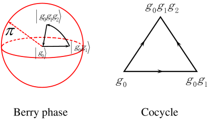
Figure 20: (Color online) Relations between Berry phase (of the end spin) in the loop ($|g_{0}\rangle,|g_{0}g_{1}\rangle,|g_{0}g_{1}g_{2}\rangle$) and 2-cocycle $\nu_{2}(g_{0},g_{0}g_{1},g_{0}g_{1}g_{2}$). In the group space of $SO(3)$, the two ends of a diameter stand for the same group element and can be seen as the same point. When $\theta=2\pi$, the Berry phase is equal to zero when the the loop intersect the shell even times and is equal to $\pi$ when the loop intersection the shell odd times. If $\theta$ is equal to even times of $2\pi$, the corresponding 2-cocycle is trivial. If $\theta$ is equal to odd times of $2\pi$, the corresponding 2-cocycle is nontrivial.

In $(2+1)$D, the possible topological $\theta$-term is the Hopf term,

$$S_{\mathrm{top}}=\theta\oint_{S_{1}\times S_{1}\times S_{1}}\hskip 1.0pt\mathrm{d}^{2}x\hskip 1.0pt\mathrm{d}\tau\varepsilon^{ijk}A_{i}F_{jk},$$ (64)

where $F_{ij}=\partial_{i}A_{j}-\partial_{j}A_{i}$, $i,j,k=x,y,\tau$. The space is compacted to $S_{1}\times S_{1}$, and the time is compacted to the last $S_{1}$. The Hopf term can be written as a total differential locally, $\varepsilon^{ijk}A_{i}F_{jk}=\varepsilon^{ijk}\partial_{k}[f_{ij}(A_{i},A_{j})]$, where $f_{ij}(A_{i},A_{j})$ is a (nonlocal) function of $A_{i}$ and $A_{j}$. Thus, at open boundary condition, the integral is determined by the boundary values, $S_{\mathrm{top}}=S_{\mathrm{L}}-S_{\mathrm{R}}$, here we have cut the space along $y$-direction. $S_{\mathrm{L}}$ is given as

$$S_{\mathrm{L}} = \theta\oint_{S_{1}\times S_{1}}\hskip 1.0pt\mathrm{d}y\hskip 1.0pt\mathrm{d}\tau(f_{y\tau}(A_{y},A_{\tau})-f_{\tau y}(A_{\tau},A_{y}))$$ (65)

$$= \theta\oint_{S^{\prime}_{1}\times S^{\prime\prime}_{1}}\hskip 1.0pt\mathrm{d}\lambda_{1}\hskip 1.0pt\mathrm{d}\lambda_{2}(\tilde{f}_{\lambda_{1}{\lambda_{2}}}(\tilde{A}_{\lambda_{1}},\tilde{A}_{\lambda_{2}})-\tilde{f}_{\lambda_{2}\lambda_{1}}(\tilde{A}_{\lambda_{2}},\tilde{A}_{\lambda_{1}}))$$

$$= \theta\int_{S_{1}^{\prime}\times D_{1}}d^{3}\lambda\varepsilon^{IJK}\tilde{A}_{I}\tilde{F}_{JK}$$

where $I,J,K=\lambda_{1},\lambda_{2},\lambda_{3}$ are parameters of the group space of $\tilde{G}$. $S_{1}^{\prime}$ is the circle formed by parameter $\lambda_{1}(y)$, and $S_{1}^{\prime\prime}$ is the circle formed by parameter $\lambda_{2}(\tau)$. $D_{1}$ is the area enclosed by the $S_{1}^{\prime\prime}$. Above we have mapped the two-dimensional integral on the boundary of space-time manifold into a three-dimensional integral on the group space of $\tilde{G}$. Notice that the spatial dimension of the boundary is 1D, the above topological $\theta$-term is actually an effective WZW term of the boundary.

Since Eq. (65) is a 3-dimensional integral over the group space of $\tilde{G}$, when reducing to the symmetry group $G$, we need at least four points to span the 3-d space $S_{1}^{\prime}\times D_{1}$: $|g_{0}\rangle,|g_{0}g_{1}\rangle,|g_{0}g_{1}g_{2}\rangle,$ and $|g_{0}g_{1}g_{2}g_{3}\rangle$. Thus we can identify Eq. (65) as a 3-cocycle or product of 3-cocycles under proper gauge choice

$$e^{iS_{L}} = \nu_{3}(g_{0},g_{0}g_{1},g_{0}g_{1}g_{2},g_{0}g_{1}g_{2}g_{3}),$$

Here $g_{0},g_{1},g_{2},g_{3}$ are group elements in the symmetry group $G$.

Above arguments can be generalized to arbitrary $d$-dimension. For example, in (1+3)D, we may have

$$S_{\text{top}}=\theta\oint_{S_{1}\times S_{3}}\hskip 1.0pt\mathrm{d}^{3}x\hskip 1.0pt\mathrm{d}\tau\varepsilon^{\mu\nu\gamma\lambda}F_{\mu\nu}F_{\gamma\lambda}.$$ (66)

The topological $\theta$-term (or $\theta$ term in literature) plays important roles in various many-body systems. In reference YL1017, , the authors came up with a new method to calculate the topological $\theta$-term.

We have shown that the topological term (or the $\theta$-term originating from Berry phase) reduce to cocycles if we discretize the space and time. The discrete topological term even exist for discrete groups (they are related to the $\theta$-term by the embedding argument mentioned previously). Although the discrete topological nonlinear sigma models constructed from group cocycle are formally close to $\theta$-terms in continuous nonlinear model, they actually describe quite different physics. The $\theta$-terms in continuous nonlinear model ignore the physics at cut-off length-scale, which should be very important in general, especially for those gapped quantum systems, whose fixed point actions have zero correlation length and quantum fluctuation can be non-smooth at arbitrary energy scale. Thus, the discrete topological nonlinear sigma models can be regarded as the quantum analogous of $\theta$-terms in continuous nonlinear sigma model and help us understand the nature of symmetry protected topological order in interacting systems.

XII SPT orders with translation symmetry

In the above we have discussed bosonic SPT phases with on-site symmetry $G$ but no other symmetries. Here we would like to stress that when we say a SPT phase have no other symmetries, we do mean that the ground state wave function of the SPT phase has no other symmetries. In fact the ground state wave function of the SPT phase can have some other symmetries. What we really mean is that when we deform the Hamiltonian to construct phase diagram, the deformed Hamiltonians can have no other symmetries.

In this section, we will discuss the SPT phases with both on-site symmetry $G$ and translation symmetry. We will use the non-linear $\sigma$-model approach to obtain our results. We have argued that the $d$-dimensional SPT phases with on-site symmetry $G$ are classified by fixed-point non-linear $\sigma$-models that contain only a topological $\theta$-term constructed from a $(1+d)$-cocycle in ${\cal H}^{1+d}[G,U_{T}(1)]$. The action-amplitude (in imaginary time) for such a fixed-point non-linear $\sigma$-model is given by

$$\hskip 1.0pt\mathrm{e}^{-\int{\cal L}^{1+d}(\nu_{1+d})}=\prod_{\{ij...k\}}\nu_{1+d}^{s_{ij...k}}(g_{i},g_{j},...,g_{k}).$$ (67)

When the system has translation symmetry, we can include additional topological $\theta$-terms which lead to richer SPT phases. Let us use (2+1)-dimensional systems as examples to discuss those addition topological $\theta$-terms.

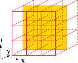
Figure 21: (Color online) A triangularization of (2+1)D space-time where each cube represent five tetrahedrons. The shaded area represents a $[xt]$ plane, on which each square represents two triangles.

When we say a (2+1)-dimensional system has a translation symmetry, we mean that the system has a discrete translation symmetry in the two spatial directions. We must choose the triangularization of the space-time in a way to be consistent with the discrete spatial translation symmetry. In this case, we can include a new topological $\theta$-term:

$$\hskip 1.0pt\mathrm{e}^{-\int{\cal L}^{3}_{\text{fix}}}=\hskip 1.0pt\mathrm{e}^{-\int{\cal L}^{3}(\nu_{3})}\hskip 1.0pt\mathrm{e}^{-\int{\cal L}^{3}(\nu^{xt}_{2})}$$ (68)

where

$$\hskip 1.0pt\mathrm{e}^{-\int{\cal L}^{3}(\nu^{xt}_{2})}=\prod_{[xt]}\prod_{\{ijk\}\in[xt]}(\nu^{xt}_{2})^{s_{ijk}}(g_{i},g_{j},g_{k}).$$ (69)

The translation invariant space-time complex can be viewed as formed by many $2$-dimensional sheets, say, in $x$-$t$ directions (see Fig. 21). We pick a sheet $[xt]$ in $x$-$t$ directions, then $\prod_{\{ijk\}\in[xt]}(\nu^{xt}_{2})^{s_{ijk}}(g_{i},g_{j},g_{k})$ is simply a topological $\theta$-term on the $[xt]$ sheet constructed from a $2$-cocycle $\nu^{xt}_{2}$ in ${\cal H}^{2}[G,U_{T}(1)]$. In the above expression, $\prod_{\{ijk\}\in[xt]}$ multiply over all triangles in the $[xt]$ sheet and $\prod_{[xt]}$ multiply over all the $[xt]$ sheets in the space-time complex.

We can include a similar topological $\theta$-term $\hskip 1.0pt\mathrm{e}^{-\int{\cal L}^{3}(\nu^{yt}_{2})}$ by considering the sheets in $y$-$t$ directions and using another 2-cocycle $\nu^{yt}_{2}$. A third topological $\theta$-term can be added by viewing space-time complex as formed by many $1$-dimensional lines in time direction:

$$\hskip 1.0pt\mathrm{e}^{-\int{\cal L}^{3}(\nu^{t}_{1})}=\prod_{[t]}\prod_{\{ij\}\in[t]}(\nu^{t}_{1})^{s_{ij}}(g_{i},g_{j}).$$ (70)

Here $\prod_{\{ij\}\in[t]}$ multiply over all segments in the $[t]$ line and $\prod_{[t]}$ multiply over all the $[t]$ lines in the space-time complex. In fact $\prod_{\{ij\}\in[t]}(\nu^{t}_{1})^{s_{ij}}(g_{i},g_{j})$ is a topological $\theta$-term on a single $[t]$ line constructed from a 1-cocycle $\nu^{t}_{1}$.

We can also try to include the fourth new topological $\theta$-term by considering the sheets in $x$-$y$ directions:

$$\hskip 1.0pt\mathrm{e}^{-\int{\cal L}^{3}(\nu^{xy}_{2})}=\prod_{[xy]}\prod_{\{ijk\}\in[xy]}(\nu^{xy}_{2})^{s_{ijk}}(g_{i},g_{j},g_{k}).$$ (71)

But such a topological $\theta$-term corresponds to a LU transformation with a few layers. In fact $\prod_{\{ijk\}\in[xy]}(\nu^{xy}_{2})^{s_{ijk}}(g_{i},g_{j},g_{k})$ is a LU transformation when viewed as a time-evolution operator. So there is no fourth new topological $\theta$-term.

We see that SPT phases in (2+1)-dimensions with an on-site symmetry $G$ and translation symmetry are characterized by one 1-cocycles $\nu^{t}_{1}\in{\cal H}^{1}[G,U_{T}(1)]$, two 2-cocycles $\nu^{xt}_{2},\nu^{yt}_{2}\in{\cal H}^{2}[G,U_{T}(1)]$, and one 3-cocycle $\nu_{3}\in{\cal H}^{3}[G,U_{T}(1)]$. If we believe that those are all the possible topological $\theta$-terms, we argue that the SPT phases in (2+1)-dimensions with an on-site symmetry $G$ and translation symmetry are classified by ${\cal H}^{1}[G,U_{T}(1)]\times{\cal H}^{2}[G,U_{T}(1)]\times{\cal H}^{2}[G,U_{T}(1)]\times{\cal H}^{3}[G,U_{T}(1)]$. A special case of this result with $\nu_{3}=0$ is discussed in LABEL:CGW1107 where the physical meaning of $\nu^{t}_{1},\nu^{xt}_{2},\nu^{yt}_{2}$ is explained in terms of 1D representations and projective representations of $G$. Certainly, the above construction can be generalized to any dimensions.

If we do not have translation symmetry, we can still add the new topological $\theta$-terms, such as $\hskip 1.0pt\mathrm{e}^{-\int{\cal L}^{3}(\nu^{xt}_{2})}$. But in this case, we can combine $n$ $[xt]$ planes in to one. If ${\cal H}^{2}[G,U_{T}(1)]$ is finite, the new topological $\theta$-term on the combined plane can be trivial if we choose $n$ properly. So, we cannot have new topological $\theta$-terms if we do not have translation symmetry and if ${\cal H}^{d}[G,U_{T}(1)]$ is finite.

XIII Summary

Since the introduction of topological order in 1989, we have been trying to gain a global and systematic understanding of topological order. We have made a lot of progress in understanding topological orders without symmetry in low dimensions. We have used the $K$-matrix to classify all Abelian fractional quantum Hall states,BW9045 ; R9002 ; WZ9290 and have used string-net condensationLW0510 ; CGW1038 to classify non-chiral topological orders in two spatial dimensions, and have constructed a large class of topological orders in higher dimensions.

The LU transformations deepen our understanding of topological order and link topological orders to patterns of long range entanglements.CGW1038 Such a deeper understanding allows us to obtain a systematic description of topological orders in 2D fermion systems.GWW1017 The LU transformations also allow us to start to understand topological order with symmetries. In particular, it allows us to classify all gapped quantum phases in one spatial dimension. We find that all gapped 1D phases are SPT phases (SPT phases are gapped quantum phases with certain symmetry which can be smoothly connected to the same trivial product state if we remove the symmetry). In 1D, the SPT phases can be classified by 2-cohomology classes of the symmetry group.

In this paper, we try to understand topological order with symmetry in higher dimensions. In particular, we try to classify SPT phases in higher dimensions. We find that distinct SPT phases with on-site symmetry $G$ in $d$ spatial dimensions can be constructed from distinct elements in $(1+d)$-Borel-cohomology classes of the symmetry group $G$. We summarize our results in table 1 for some simple symmetry groups.

We have used two approaches to obtain the above result: the LU transformations and topological non-linear $\sigma$-models. We generalized the usual topological $\theta$-term and the WZW term in continuous non-linear $\sigma$-model to the topological $\theta$-term and the NLL terms in lattice non-linear $\sigma$-models (with both discrete space-time and discrete target space).

Our results demonstrate how many-body entanglements interact with symmetry in a simple situation where there is no long range entanglements (ie no intrinsic topological orders). This may prepare us to study the more important and harder problem: how to classify quantum states with long range entanglements (ie with intrinsic topological orders) and symmetry. Those phases with long range entanglements and symmetry are called symmetry enriched topological orders. Also, our approach can be modified and generalized to describe/classify fermionic SPT phases, through generalizing the group cohomology theory to group super-cohomology theory.GW

XIV Acknowledgements

X.G.W. would like to thank Michael Levin for helpful discussions and for sharing his result of bosonic SPT phases in $(2+1)$-dimensions.LU1 This motivated us to calculate ${\cal H}^{1+d}[U(1),U(1)]$, which reproduced his results for $d=2$. We would like to thank Geoffrey Lee, Jian-Zhong Pan, and Zhenghan Wang for many very helpful discussions on group cohomology for discrete and continuous groups. Z.C.G. would like to thank Dung-Hai Lee for discussion on the possibility of discretized Berry phase term in $1+1$D. This research is supported by NSF Grant No. DMR-1005541 and NSFC 11074140. Z.C.G. is supported by NSF Grant No. PHY05-51164.

Appendix A Making the condition eqn. (12) a local condition

We can make the condition eqn. (12) on $U^{\bm{i}}$ a local condition. Instead of requiring eqn. (12), we may require $U^{\bm{i}}$ to satisfy

$$\ \ \ \ (U^{\bm{i}}\otimes U^{\bm{i}+\bm{x}}\otimes U^{\bm{i}+\bm{y}}\otimes U^{\bm{i}+\bm{x}+\bm{y}})(P^{\bm{i}}\otimes p^{\bm{i}})$$ (72)

$$=(P^{\bm{i}}\otimes p^{\bm{i}})(U^{\bm{i}}\otimes U^{\bm{i}+\bm{x}}\otimes U^{\bm{i}+\bm{y}}\otimes U^{\bm{i}+\bm{x}+\bm{y}})(P^{\bm{i}}\otimes p^{\bm{i}})$$

for certain projection operators $P^{\bm{i}}$ and $p^{\bm{i}}$ with Tr$p^{\bm{i}}=1$. Here $U^{\bm{i}}\otimes U^{\bm{i}+\bm{x}}\otimes U^{\bm{i}+\bm{y}}\otimes U^{\bm{i}+\bm{x}+\bm{y}}$ and $P^{\bm{i}}\otimes p^{\bm{i}}$ are matrices given by

$$\ \ \ \ (U^{\bm{i}}\otimes U^{\bm{i}+\bm{x}}\otimes U^{\bm{i}+\bm{y}}\otimes U^{\bm{i}+\bm{x}+\bm{y}})$$

$$\to U^{\bm{i}}_{\alpha_{1}\alpha_{2}\alpha_{3}\alpha_{4},\alpha_{1}^{\prime}\alpha_{2}^{\prime}\alpha_{3}^{\prime}\alpha_{4}^{\prime}}U^{\bm{i}+\bm{x}}_{\beta_{1}\beta_{2}\beta_{3}\beta_{4},\beta_{1}^{\prime}\beta_{2}^{\prime}\beta_{3}^{\prime}\beta_{4}^{\prime}}\times$$

$$\ \ \ \ \ \ \ \ \ \ \ \ \ \ \ \ \ \ U^{\bm{i}+\bm{y}}_{\gamma_{1}\gamma_{2}\gamma_{3}\gamma_{4},\gamma_{1}^{\prime}\gamma_{2}^{\prime}\gamma_{3}^{\prime}\gamma_{4}^{\prime}}U^{\bm{i}+\bm{x}+\bm{y}}_{\lambda_{1}\lambda_{2}\lambda_{3}\lambda_{4},\lambda_{1}^{\prime}\lambda_{2}^{\prime}\lambda_{3}^{\prime}\lambda_{4}^{\prime}}$$ (73)

and

$$(P^{\bm{i}}\otimes p^{\bm{i}})\to p^{\bm{i}}_{\alpha_{1}\beta_{2}\gamma_{3}\lambda_{4},\alpha_{1}^{\prime}\beta_{2}^{\prime}\gamma_{3}^{\prime}\lambda_{4}^{\prime}}\times$$ (74)

$$\ \ \ \ P^{\bm{i}}_{\alpha_{2}\alpha_{3}\alpha_{4}\beta_{1}\beta_{3}\beta_{4}\gamma_{1}\gamma_{2}\gamma_{4}\lambda_{1}\lambda_{2}\lambda_{3},\alpha_{2}^{\prime}\alpha_{3}^{\prime}\alpha_{4}^{\prime}\beta_{1}^{\prime}\beta_{3}^{\prime}\beta_{4}^{\prime}\gamma_{1}^{\prime}\gamma_{2}^{\prime}\gamma_{4}^{\prime}\lambda_{1}^{\prime}\lambda_{2}^{\prime}\lambda_{3}^{\prime}},$$

The condition eqn. (12) implies the condition eqn. (72) because, in the canonical form, the states on the sites $\alpha_{1},\ \beta_{2},\ \gamma_{3},\ \lambda_{4}$ and the states on the sites $\alpha_{2},\ \alpha_{3},\ \alpha_{4},\ \beta_{1},\ \beta_{3},\ \beta_{4},\ \gamma_{1},\ \gamma_{2},\ \gamma_{4},\ \lambda_{1},\ \lambda_{2},\ \lambda_{3}$ are unentangled (see Fig. 8).

Appendix B Representations and projective Representations

Let us consider a group $G$ that may contain anti-unitary time reversal transformation. We can divide the group elements into two classes:

$$s(g)=1\text{ or }-1,\ \ \ \ g\in G.$$ (75)

The group elements that contain an odd number of time-reversal operations have $s(g)=-1$ and the group elements that contain an even number of time-reversal operations have $s(g)=1$.

Unitary matrices $u(g)$ form a representation of symmetry group $G$ if

$$u(g_{1})u_{s(g_{1})}(g_{2})=u(g_{1}g_{2}).$$ (76)

where $u_{s(g_{1})}(g_{2})=u(g_{2})$ if $s(g_{1})=1$ and $u_{s(g_{1})}(g_{2})=[u(g_{2})]^{*}$ if $s(g_{1})=-1$.

The above relation is obtained from the following mapping

$$g\to u(g),\text{ if }s(g)=1;\ \ \ \ g\to u(g)K,\text{ if }s(g)=-1.$$ (77)

Here $K$ is the anti-unitary operator

$$Ka=a^{*}K,$$ (78)

where $a$ is a complex number. For example, if $s(g_{1})=s(g_{2})=-1$ and $s(g_{1}g_{2})=1$, we require that

$$u(g_{1})Ku(g_{2})K=u(g_{1}g_{2})$$ (79)

which leads to eqn. (76).

Matrices $u(g)$ form a projective representation of symmetry group $G$ if

$$u(g_{1})u_{s(g_{1})}(g_{2})=\omega(g_{1},g_{2})u(g_{1}g_{2}),\ \ \ \ \ g_{1},g_{2}\in G.$$ (80)

Here $\omega(g_{1},g_{2})\in U(1)$ and $\omega(g_{1},g_{2})\neq 0$, which is called the factor system of the projective representation. The associativity requires that

$$[u(g_{1})u_{s(g_{1})}(g_{2})]u_{s(g_{1}g_{2})}(g_{3})=u(g_{1})[u(g_{2})u_{s(g_{2})}(g_{3})]_{s(g_{1})}$$ (81)

or

$$\ \ \ \ \omega(g_{1},g_{2})\omega(g_{1}g_{2},g_{3})u(g_{1}g_{2}g_{3})$$

$$=\omega^{s(g_{1})}(g_{2},g_{3})\omega(g_{1},g_{2}g_{3})u(g_{1}g_{2}g_{3})$$ (82)

Thus, the factor system satisfies

$$\omega^{s(g_{1})}(g_{2},g_{3})\omega(g_{1},g_{2}g_{3}) =\omega(g_{1},g_{2})\omega(g_{1}g_{2},g_{3}),$$ (83)

for all $g_{1},g_{2},g_{3}\in G$. If $\omega(g_{1},g_{2})=1$, $u(g)$ reduces to the usual linear representation of $G$.

A different choice of pre-factor for the representation matrices $u^{\prime}(g)=\beta(g)u(g)$ will lead to a different factor system $\omega^{\prime}(g_{1},g_{2})$:

$$\omega^{\prime}(g_{1},g_{2})=\frac{\beta(g_{1}g_{2})}{\beta(g_{1})\beta^{s(g_{1})}(g_{2})}\omega(g_{1},g_{2}).$$ (84)

We regard $u^{\prime}(g)$ and $u(g)$ that differ only by a pre-factor as equivalent projective representations and the corresponding factor systems $\omega^{\prime}(g_{1},g_{2})$ and $\omega(g_{1},g_{2})$ as belonging to the same class $\omega$.

Suppose that we have one projective representation $u_{1}(g)$ with factor system $\omega_{1}(g_{1},g_{2})$ of class $\omega_{1}$ and another $u_{2}(g)$ with factor system $\omega_{2}(g_{1},g_{2})$ of class $\omega_{2}$, obviously $u_{1}(g)\otimes u_{2}(g)$ is a projective presentation with factor group $\omega_{1}(g_{1},g_{2})\omega_{2}(g_{1},g_{2})$. The corresponding class $\omega$ can be written as a sum $\omega_{1}+\omega_{2}$. Under such an addition rule, the equivalence classes of factor systems form an Abelian group, which is called the second cohomology group of $G$ and denoted as ${\cal H}^{2}[G,U_{T}(1)]$. The “zero” element $0\in{\cal H}^{2}[G,U_{T}(1)]$ is the class that corresponds to the linear representation of the group. The best known example of projective representation is the spin-1/2 representation of $SO(3)$. The integer spins correspond to the linear representations of $SO(3)$.

Appendix C 1D representations and projective representations of $U(1)\times Z_{2}$ and $U(1)\rtimes Z_{2}$

In this section, we are going to discuss the 1D representations and projective representations of four groups $U(1)\times Z_{2}$, $U(1)\rtimes Z_{2}$, $U(1)\times Z_{2}^{T}$, and $U(1)\rtimes Z_{2}^{T}$. As group, $Z_{2}$ and $Z_{2}^{T}$ are actually the same group. However, the generator $t$ of $Z_{2}$ corresponds to a usual symmetry transformation which has a unitary representation. The generator $T$ of $Z_{2}^{T}$ corresponds to the time reversal transformation which has a anti-unitary representation.

Let $U_{\theta}$, $\theta\in[0,2\pi)$, be an element in $U(1)$. The four groups are defined by the following relations

$$U(1)\times Z_{2}:\ \ tU_{\theta}=U_{\theta}t;$$

$$U(1)\times Z_{2}^{T}:\ \ TU_{\theta}=U_{\theta}T;$$

$$U(1)\rtimes Z_{2}:\ \ tU_{\theta}=U_{-\theta}t;$$

$$U(1)\rtimes Z_{2}^{T}:\ \ TU_{\theta}=U_{-\theta}T.$$ (85)

Their representations are given by matrix functions $M(U_{\theta})$ and $M(t)$ (or $M(T)K$).

A 1D representation of $U(1)\times Z_{2}$ has a form

$$M(U_{\theta})=\hskip 1.0pt\mathrm{e}^{n\hskip 1.0pt\mathrm{i}\hskip 1.0pt\theta},\ \ \ M(t)=\eta=\pm 1,$$ (86)

where $n\in\mathbb{Z}$. One can check that $M(T)M(U_{\theta})=M(U_{\theta})M(T)$, for any $n$. So the 1D representation of $U(1)\times Z_{2}$ is labeled by $n$ and $\eta$ (or by $\mathbb{Z}\times\mathbb{Z}_{2}$).

A 1D representation of $U(1)\rtimes Z_{2}$ also has a form eqn. (86) One can check that $M(T)M(U_{\theta})=M(U_{-\theta})M(T)$ only when $n=0$. So there are two 1D representation of $U(1)\rtimes Z_{2}$ labeled by $\mathbb{Z}_{2}$ (corresponding to $\eta=\pm 1$).

A 1D representation of $U(1)\times Z_{2}^{T}$ has a form

$$M(U_{\theta})=\hskip 1.0pt\mathrm{e}^{n\hskip 1.0pt\mathrm{i}\hskip 1.0pt\theta},\ \ \ M(T)K=\hskip 1.0pt\mathrm{e}^{\hskip 1.0pt\mathrm{i}\hskip 1.0pt\phi}K,$$ (87)

where $n\in\mathbb{Z}$ and $\phi\in\mathbb{R}$. Note that $M(T)KM(T)K=1$ for any $\phi$. We find

$$\ \ \ \ M(T)KM(U_{\theta})=M(T)K\hskip 1.0pt\mathrm{e}^{n\hskip 1.0pt\mathrm{i}\hskip 1.0pt\theta}$$

$$=\hskip 1.0pt\mathrm{e}^{-n\hskip 1.0pt\mathrm{i}\hskip 1.0pt\theta}M(T)K.$$ (88)

Thus $M(T)KM(U_{\theta})=M(U_{\theta})M(T)K$ only when $n=0$. Also under an unitary transformation $\hskip 1.0pt\mathrm{e}^{\hskip 1.0pt\mathrm{i}\hskip 1.0pt\phi}$, $M(T)K$ transforms as

$$\hskip 1.0pt\mathrm{e}^{\hskip 1.0pt\mathrm{i}\hskip 1.0pt\phi}(\hskip 1.0pt\mathrm{e}^{\hskip 1.0pt\mathrm{i}\hskip 1.0pt\phi}K)\hskip 1.0pt\mathrm{e}^{-\hskip 1.0pt\mathrm{i}\hskip 1.0pt\phi}=\hskip 1.0pt\mathrm{e}^{\hskip 1.0pt\mathrm{i}\hskip 1.0pt(\phi+2\varphi)}K.$$ (89)

So different $\phi$ correspond to the same 1D representation. Therefore, there is only one 1D representation for $U(1)\times Z_{2}^{T}$.

From the above calculation, we note that $M(T)K|n\rangle\propto|-n\rangle$ where $|n\rangle$ is an eigenstate of $M(U_{\theta})$: $M(U_{\theta})|n\rangle=\hskip 1.0pt\mathrm{e}^{n\hskip 1.0pt\mathrm{i}\hskip 1.0pt\theta}|n\rangle$. So the group $Z_{2}^{T}\times U(1)$ describes the symmetry group of a spin system with time reversal and $S_{z}$ spin rotation symmetry (the $U(1)$ symmetry).

A 1D representation of $U(1)\rtimes Z_{2}^{T}$ also has a form eqn. (87). We find

$$\ \ \ \ M(T)KM(U_{\theta})=M(T)K\hskip 1.0pt\mathrm{e}^{n\hskip 1.0pt\mathrm{i}\hskip 1.0pt\theta}$$

$$=\hskip 1.0pt\mathrm{e}^{-n\hskip 1.0pt\mathrm{i}\hskip 1.0pt\theta}M(T)K=M(U_{-\theta})M(T)K.$$ (90)

Thus $M(T)KM(U_{\theta})=M(U_{-\theta})M(T)K$ for any $n\in\mathbb{Z}$, and the 1D representations for $U(1)\rtimes Z_{2}^{T}$ are labeled by $\mathbb{Z}$.

The above relation (C) also allows us to show $M(T)K|n\rangle\propto|n\rangle$, where $|n\rangle$ is an eigenstate of $M(U_{\theta})$: $M(U_{\theta})|n\rangle=\hskip 1.0pt\mathrm{e}^{n\hskip 1.0pt\mathrm{i}\hskip 1.0pt\theta}|n\rangle$. This is the expected transformation of time reversal for boson systems, where $n$ is the boson number. Therefore $U(1)\rtimes Z_{2}^{T}$ is the symmetry group of boson systems with time reversal symmetry and boson number conservation.

Next, let us discuss the projective representations of the four groups. First, let us consider $U(1)\times Z_{2}$, whose projective representations may have a form

$$M(U_{\theta})=\begin{pmatrix}\hskip 1.0pt\mathrm{e}^{n\hskip 1.0pt\mathrm{i}\hskip 1.0pt\theta}&0\\ 0&\hskip 1.0pt\mathrm{e}^{m\hskip 1.0pt\mathrm{i}\hskip 1.0pt\theta}\\ \end{pmatrix},\ \ \ M(T)=\begin{pmatrix}0&1\\ 1&0\end{pmatrix}.$$ (91)

One can check

$$M(T)M(U_{\theta}) =\begin{pmatrix}0&\hskip 1.0pt\mathrm{e}^{m\hskip 1.0pt\mathrm{i}\hskip 1.0pt\theta}\\ \hskip 1.0pt\mathrm{e}^{n\hskip 1.0pt\mathrm{i}\hskip 1.0pt\theta}&0\end{pmatrix},$$

$$M(U_{\theta})M(T) =\begin{pmatrix}0&\hskip 1.0pt\mathrm{e}^{n\hskip 1.0pt\mathrm{i}\hskip 1.0pt\theta}\\ \hskip 1.0pt\mathrm{e}^{m\hskip 1.0pt\mathrm{i}\hskip 1.0pt\theta}&0\end{pmatrix}.$$ (92)

$M(T)M(U_{\theta})$ and $M(U_{\theta})M(T)$ differ by a total phase only when $m=n\in\mathbb{Z}$, in that case $M(T)M(U_{\theta})=M(U_{\theta})M(T)$. Note that $M(T)M(T)=1$. So we have a trivial projective representation. If we choose $M(T)=\begin{pmatrix}0&1\\ 1&0\end{pmatrix}$, we will have $M(T)M(T)=-1$. But we still have a trivial projective representations, since if we add an phase factor $\tilde{M}(T)=\hskip 1.0pt\mathrm{i}\hskip 1.0ptM(T)$, we have $\tilde{M}(T)\tilde{M}(T)=-1$ Thus $U(1)\times Z_{2}$ has only one trivial class of projective representations.

Second, let us consider the projective representations for $U(1)\rtimes Z_{2}$, which may have a form

$$M(U_{\theta})=\begin{pmatrix}\hskip 1.0pt\mathrm{e}^{n\hskip 1.0pt\mathrm{i}\hskip 1.0pt\theta}&0\\ 0&\hskip 1.0pt\mathrm{e}^{m\hskip 1.0pt\mathrm{i}\hskip 1.0pt\theta}\\ \end{pmatrix},\ \ \ M(T)=\begin{pmatrix}0&1\\ 1&0\end{pmatrix}.$$ (93)

One can check

$$M(T)M(U_{\theta}) =\begin{pmatrix}0&\hskip 1.0pt\mathrm{e}^{m\hskip 1.0pt\mathrm{i}\hskip 1.0pt\theta}\\ \hskip 1.0pt\mathrm{e}^{n\hskip 1.0pt\mathrm{i}\hskip 1.0pt\theta}&0\end{pmatrix},$$

$$M(U_{-\theta})M(T) =\begin{pmatrix}0&\hskip 1.0pt\mathrm{e}^{-n\hskip 1.0pt\mathrm{i}\hskip 1.0pt\theta}\\ \hskip 1.0pt\mathrm{e}^{-m\hskip 1.0pt\mathrm{i}\hskip 1.0pt\theta}&0\end{pmatrix}.$$ (94)

We have

$$M(T)M(U_{\theta})=\hskip 1.0pt\mathrm{e}^{-(n+m)\hskip 1.0pt\mathrm{i}\hskip 1.0pt\theta}M(U_{-\theta})M(T)$$ (95)

Also note that $M(T)M(T)=1$. So we have a non-trivial projective representation. If we add a phase factor $\tilde{M}(U_{\theta})=\hskip 1.0pt\mathrm{e}^{k\hskip 1.0pt\mathrm{i}\hskip 1.0pt\theta}M(U_{\theta})$, we will have

$$M(T)\tilde{M}(U_{\theta})=\hskip 1.0pt\mathrm{e}^{-(n+m-2k)\hskip 1.0pt\mathrm{i}\hskip 1.0pt\theta}\tilde{M}(U_{-\theta})M(T)$$ (96)

So the projective representations with different $n$ and $m$ belong to two classes $m+n$ = even and $m+n=$ odd. Thus $U(1)\rtimes Z_{2}$ has two classes of projective representations labeled by $\mathbb{Z}_{2}$.

The projective representation of $U(1)\times Z_{2}^{T}$ can have a form

$$U_{\theta} \to M(U_{\theta})=\begin{pmatrix}\hskip 1.0pt\mathrm{e}^{n\hskip 1.0pt\mathrm{i}\hskip 1.0pt\theta}&0\\ 0&\hskip 1.0pt\mathrm{e}^{m\hskip 1.0pt\mathrm{i}\hskip 1.0pt\theta}\\ \end{pmatrix},$$

$$T \to M(T)K=\begin{pmatrix}0&1\\ 1&0\end{pmatrix}K.$$ (97)

One can check

$$M(T)KM(U_{\theta}) =\begin{pmatrix}0&\hskip 1.0pt\mathrm{e}^{-m\hskip 1.0pt\mathrm{i}\hskip 1.0pt\theta}\\ \hskip 1.0pt\mathrm{e}^{-n\hskip 1.0pt\mathrm{i}\hskip 1.0pt\theta}&0\end{pmatrix}K$$

$$M(U_{\theta})M(T)K =\begin{pmatrix}0&\hskip 1.0pt\mathrm{e}^{n\hskip 1.0pt\mathrm{i}\hskip 1.0pt\theta}\\ \hskip 1.0pt\mathrm{e}^{m\hskip 1.0pt\mathrm{i}\hskip 1.0pt\theta}&0\end{pmatrix}K.$$ (98)

We have

$$M(T)KM(U_{\theta})=\hskip 1.0pt\mathrm{e}^{-(n+m)\hskip 1.0pt\mathrm{i}\hskip 1.0pt\theta}M(U_{\theta})M(T)K$$ (99)

Note that $M(T)KM(T)K=1$. So we have a projective representation when $m,n\in\mathbb{Z}$ . If we add a phase factor $\tilde{M}(U_{\theta})=\hskip 1.0pt\mathrm{e}^{k\hskip 1.0pt\mathrm{i}\hskip 1.0pt\theta}M(U_{\theta})$, then

$$M(T)K\tilde{M}(U_{\theta})=\hskip 1.0pt\mathrm{e}^{-(n+m+2k)\hskip 1.0pt\mathrm{i}\hskip 1.0pt\theta}\tilde{M}(U_{\theta})M(T)K.$$ (100)

So the above projective representations belong to two classes: $m+n=$ even and $m+n=$ odd.

The projective representation of $Z_{2}^{T}\times U(1)$ may also have a form

$$M(U_{\theta})=\begin{pmatrix}\hskip 1.0pt\mathrm{e}^{n\hskip 1.0pt\mathrm{i}\hskip 1.0pt\theta}&0\\ 0&\hskip 1.0pt\mathrm{e}^{m\hskip 1.0pt\mathrm{i}\hskip 1.0pt\theta}\\ \end{pmatrix},\ \ \ M(T)K=\begin{pmatrix}0&-1\\ 1&0\end{pmatrix}K.$$ (101)

One can check

$$M(T)KM(U_{\theta}) =\begin{pmatrix}0&-\hskip 1.0pt\mathrm{e}^{-m\hskip 1.0pt\mathrm{i}\hskip 1.0pt\theta}\\ \hskip 1.0pt\mathrm{e}^{-n\hskip 1.0pt\mathrm{i}\hskip 1.0pt\theta}&0\end{pmatrix}K,$$

$$M(U_{\theta})M(T)K =\begin{pmatrix}0&-\hskip 1.0pt\mathrm{e}^{n\hskip 1.0pt\mathrm{i}\hskip 1.0pt\theta}\\ \hskip 1.0pt\mathrm{e}^{m\hskip 1.0pt\mathrm{i}\hskip 1.0pt\theta}&0\end{pmatrix}K.$$ (102)

We have

$$M(T)KM(U_{\theta})=\hskip 1.0pt\mathrm{e}^{-(n+m)\hskip 1.0pt\mathrm{i}\hskip 1.0pt\theta}M(U_{\theta})M(T)K$$ (103)

Note that $M(T)KM(T)K=-1$. So we also have a projective representation when $m,n\in\mathbb{Z}$ . Those projective representations also belong to two classes: $m+n=$ even and $m+n=$ odd. So $U(1)\times Z_{2}^{T}$ has four classes of projective representations labeled by $\mathbb{Z}_{2}\times\mathbb{Z}_{2}$.

For the $U(1)\rtimes Z_{2}^{T}$ group, its projective representation may have a form

$$M(U_{\theta})=\begin{pmatrix}\hskip 1.0pt\mathrm{e}^{n\hskip 1.0pt\mathrm{i}\hskip 1.0pt\theta}&0\\ 0&\hskip 1.0pt\mathrm{e}^{m\hskip 1.0pt\mathrm{i}\hskip 1.0pt\theta}\\ \end{pmatrix},\ \ \ M(T)K=\begin{pmatrix}0&-1\\ 1&0\end{pmatrix}K.$$ (104)

One can check

$$M(T)KM(U_{\theta}) =\begin{pmatrix}0&-\hskip 1.0pt\mathrm{e}^{-m\hskip 1.0pt\mathrm{i}\hskip 1.0pt\theta}\\ \hskip 1.0pt\mathrm{e}^{-n\hskip 1.0pt\mathrm{i}\hskip 1.0pt\theta}&0\end{pmatrix}K,$$

$$M(U_{-\theta})M(T)K =\begin{pmatrix}0&-\hskip 1.0pt\mathrm{e}^{-n\hskip 1.0pt\mathrm{i}\hskip 1.0pt\theta}\\ \hskip 1.0pt\mathrm{e}^{-m\hskip 1.0pt\mathrm{i}\hskip 1.0pt\theta}&0\end{pmatrix}K.$$ (105)

$M(T)KM(U_{\theta})$ and $M(U_{\theta})M(T)K$ differ by a total phase only when $m=n\in\mathbb{Z}$. Note that $M(T)KM(T)K=-1$. If we add a phase factor $\tilde{M}(T)=\hskip 1.0pt\mathrm{e}^{\hskip 1.0pt\mathrm{i}\hskip 1.0pt\phi}M(T)$, we still have $\tilde{M}(T)K\tilde{M}(T)K=-1$ So we have a non-trivial projective representation. Those projective representations for different $n=m$ all belong to one class. Thus $U(1)\rtimes Z_{2}^{T}$ has two classes of projective representations (the one discussed above plus the trivial one) labeled by $\mathbb{Z}_{2}$.

Appendix D Group cohomology

The above discussion on the factor system of a projective representation can be generalized which give rise to a cohomology theory of group. In this section, we will briefly describe the group cohomology theory.RS

D.1 $G$-module

For a group $G$, let $M$ be a $G$-module, which is an Abelian group (with multiplication operation) on which $G$ acts compatibly with the multiplication operation (ie the Abelian group structure):

$$g\cdot(ab)=(g\cdot a)(g\cdot b),\ \ \ \ g\in G,\ \ \ \ a,b\in M.$$ (106)

For the most cases studied in this paper, $M$ is simply the $U(1)$ group and $a$ an $U(1)$ phase. The multiplication operation $ab$ is the usual multiplication of the $U(1)$ phases. The group action is trivial: $g\cdot a=a$, $g\in G$, $a\in U(1)$. We will denote such a trivial $G$-module as $M=U(1)$.

For a group $G$ that contain time-reversal operation, we can define a non-trivial $G$-module which is denoted as $U_{T}(1)$. $U_{T}(1)$ is also a $U(1)$ group whose elements are the $U(1)$ phases. The multiplication operation $ab$, $a,b\in U_{T}(1)$, is still the usual multiplication of the $U(1)$ phases. However, the group action is non-trivial now: $g\cdot a=a^{s(g)}$, $g\in G$, $a\in U_{T}(1)$, where $s(g)=1$ if $g$ contains no anti-unitary time reversal transformation $T$ and $s(g)=-1$ if $g$ contains one anti-unitary time reversal transformation $T$.

The module defined above is actually a model over a ring $\mathbb{Z}$, since we have the following operation $\mathbb{Z}\times M\to M$:

$$\forall n\in\mathbb{Z},\forall a\in M,\ \ \ a^{n}\in M.$$ (107)

A model $M$ can be over a more general ring $R$ if we have the operation $R\times M\to M$:

$$\forall n\in,\forall a\in M,\ \ \ a^{n}\in M,$$ (108)

such that

$$a^{n}b^{n}=(ab)^{n},\ a^{n}a^{m}=a^{m+n},\ a^{nm}=(a^{m})^{n},\ a^{1_{R}}=a,$$ (109)

if $R$ has multiplicative identity $1_{R}$.

Such a general concept of a module over a ring is a generalization of the notion of vector space, wherein the corresponding scalars are allowed to lie in an arbitrary ring. As we have seen, modules also generalize the notion of Abelian groups, which are modules over the ring of integers

D.2 Algebraic definition of group cohomology

Let $\omega_{n}(g_{1},...,g_{n})$ be a function of $n$ group elements whose value is in the $G$-module $M$. In other words, $\omega_{n}:G^{n}\to M$. Let ${\cal C}^{n}(G,M)=\{\omega_{n}\}$ be the space of all such functions. Note that ${\cal C}^{n}(G,M)$ is an Abelian group under the function multiplication $\omega^{\prime\prime}_{n}(g_{1},...,g_{n})=\omega_{n}(g_{1},...,g_{n})\omega^{\prime}_{n}(g_{1},...,g_{n})$. We define a map $d_{n}$ from ${\cal C}^{n}[G,U_{T}(1)]$ to ${\cal C}^{n+1}[G,U_{T}(1)]$:

$$\ \ \ \ (d_{n}\omega_{n})(g_{1},...,g_{n+1})=$$

$$[g_{1}\cdot\omega_{n}(g_{2},...,g_{n+1})]\omega_{n}^{(-1)^{n+1}}(g_{1},...,g_{n})\times$$

$$\ \ \ \ \ \prod_{i=1}^{n}\omega_{n}^{(-1)^{i}}(g_{1},...,g_{i-1},g_{i}g_{i+1},g_{i+2},...g_{n+1})$$ (110)

Let

$${\cal B}^{n}(G,M)=\{\omega_{n}|\omega_{n}=d_{n-1}\omega_{n-1}|\omega_{n-1}\in{\cal C}^{n-1}(G,M)\}$$ (111)

and

$${\cal Z}^{n}(G,M)=\{\omega_{n}|d_{n}\omega_{n}=1,\omega_{n}\in{\cal C}^{n}(G,M)\}$$ (112)

${\cal B}^{n}(G,M)$ and ${\cal Z}^{n}(G,M)$ are also Abelian groups which satisfy ${\cal B}^{n}(G,M)\subset{\cal Z}^{n}(G,M)$ where ${\cal B}^{1}(G,M)\equiv\{1\}$. The $n$-cocycle of $G$ is defined as

$${\cal H}^{n}(G,M)={\cal Z}^{n}(G,M)/{\cal B}^{n}(G,M)$$ (113)

Let us discuss some examples. We choose $M=U_{T}(1)$ and $G$ acts as: $g\cdot a=a^{s(g)}$, $g\in G$, $a\in U_{T}(1)$. In this case $\omega_{n}(g_{1},...,g_{n})$ is just a phase factor. From

$$(d_{0}\omega_{0})(g_{1})=\omega_{0}^{s(g_{1})}/\omega_{0}$$ (114)

we see that

$${\cal Z}^{0}[G,U_{T}(1)]=\{\omega_{0}|\omega_{0}^{s(g_{1})}=\omega_{0}\}\equiv U_{T}^{G}(1)$$ (115)

If $G$ contain time reversal, $U_{T}^{G}(1)=\{1,-1\}$. If $G$ does not contain time reversal, $U_{T}^{G}(1)=U(1)$. Since ${\cal B}^{0}[G,U_{T}(1)]\equiv\{1\}$ is trivial, we obtain ${\cal H}^{0}[G,U_{T}(1)]=U_{T}^{G}(1)$.

From

$$(d_{1}\omega_{1})(g_{1},g_{2})=\omega_{1}^{s(g_{1})}(g_{2})\omega_{1}(g_{1})/\omega_{1}(g_{1}g_{2})$$ (116)

we see that

$${\cal Z}^{1}[G,U_{T}(1)]=\{\omega_{1}|\omega_{1}(g_{1})\omega_{1}^{s(g_{1})}(g_{2})=\omega_{1}(g_{1}g_{2})\}.$$ (117)

Also

$${\cal B}^{1}[G,U_{T}(1)]=\{\omega_{1}|\omega_{1}(g_{1})=\omega_{0}^{s(g_{1})}/\omega_{0}\}$$ (118)

${\cal H}^{1}[G,U_{T}(1)]={\cal Z}^{1}[G,U_{T}(1)]/{\cal B}^{1}[G,U_{T}(1)]$ is the set of all the inequivalent 1D representations of $G$.

From

$$\ \ \ \ (d_{2}\omega_{2})(g_{1},g_{2},g_{3})$$ (119)

$$=\omega_{2}^{s(g_{1})}(g_{2},g_{3})\omega_{2}(g_{1},g_{2}g_{3})/\omega_{2}(g_{1}g_{2},g_{3})\omega_{2}(g_{1},g_{2})$$

we see that

$${\cal Z}^{2}[G,U_{T}(1)]=\{\omega_{2}|$$ (120)

$$\ \ \ \omega_{2}(g_{1},g_{2}g_{3})\omega_{2}^{s(g_{1})}(g_{2},g_{3})=\omega_{2}(g_{1}g_{2},g_{3})\omega_{2}(g_{1},g_{2})\}.$$

and

$${\cal B}^{2}[G,U_{T}(1)]=\{\omega_{2}|\omega_{2}(g_{1},g_{2})=\omega_{1}^{s(g_{1})}(g_{2})\omega_{1}(g_{1})/\omega_{1}(g_{1}g_{2})\}.$$ (121)

The 2-cohomology group ${\cal H}^{2}[G,U_{T}(1)]={\cal Z}^{2}[G,U_{T}(1)]/{\cal B}^{2}[G,U_{T}(1)]$ classify the projective representations discussed in section B.

From

$$\ \ \ \ (d_{3}\omega_{3})(g_{1},g_{2},g_{3},g_{4})$$

$$=\frac{\omega_{3}^{s(g_{1})}(g_{2},g_{3},g_{4})\omega_{3}(g_{1},g_{2}g_{3},g_{4})\omega_{3}(g_{1},g_{2},g_{3})}{\omega_{3}(g_{1}g_{2},g_{3},g_{4})\omega_{3}(g_{1},g_{2},g_{3}g_{4})}$$ (122)

we see that

$${\cal Z}^{3}[G,U_{T}(1)]=\{\omega_{3}|$$ (123)

$$\ \ \ \frac{\omega_{3}^{s(g_{1})}(g_{2},g_{3},g_{4})\omega_{3}(g_{1},g_{2}g_{3},g_{4})\omega_{3}(g_{1},g_{2},g_{3})}{\omega_{3}(g_{1}g_{2},g_{3},g_{4})\omega_{3}(g_{1},g_{2},g_{3}g_{4})}=1\}.$$

and

$$\ \ \ \ {\cal B}^{3}[G,U_{T}(1)]$$ (124)

$$=\{\omega_{3}|\omega_{3}(g_{1},g_{2},g_{3})=\frac{\omega_{2}^{s(g_{1})}(g_{2},g_{3})\omega_{2}(g_{1},g_{2}g_{3})}{\omega_{2}(g_{1}g_{2},g_{3})\omega_{2}(g_{1},g_{2})}\},$$

which give us the 3-cohomology group ${\cal H}^{3}[G,U_{T}(1)]={\cal Z}^{3}[G,U_{T}(1)]/{\cal B}^{3}[G,U_{T}(1)]$.

In this paper, we will show that ${\cal H}^{1+d}[G,U_{T}(1)]$ can classify SPT phases in $d$-spatial dimensions with an on-site unitary symmetry group $G$. Here the on-site symmetry group $G$ may contain time-reversal operations.

D.3 Geometric interpretation of group cohomology

In the following, we will describe a geometric interpretation of group cohomology. First, let us introduce the map $\nu_{n}:G^{n+1}\to M$ that satisfy

$$g\cdot\nu_{n}(g_{0},g_{1},...,g_{n})=\nu_{n}(gg_{0},gg_{1},...,gg_{n}),$$ (125)

for any $g\in G$. We will call such a map $\nu_{n}$ a $n$-cochain:

$${\cal C}^{n}(G,M)=\{\nu_{n}|g\cdot\nu_{n}(g_{0},...,g_{n})=\nu_{n}(gg_{0},...,gg_{n})\}.$$ (126)

$\omega_{n}$ discussed above is one-to-one related to $\nu_{n}$ through

$$\omega_{n}(g_{1},...,g_{n}) =\nu_{n}(1,g_{1},g_{1}g_{2},...,g_{1}\cdots g_{n})$$

$$=\nu_{n}(1,\tilde{g}_{1},\tilde{g}_{2},...,\tilde{g}_{n})$$ (127)

where $\tilde{g}_{i}=g_{1}g_{2}\cdots g_{i}$.

We can rewrite the $d_{n}$ map, $d_{n}:\omega_{n}\to\omega_{n+1}$, as $d_{n}:\nu_{n}\to\nu_{n+1}$:

$$\ \ \ \ (d_{n}\nu_{n})(1,g_{1},g_{1}g_{2},...,g_{1}\cdots g_{n+1})$$

$$=g_{1}\cdot\nu_{n}(1,g_{2},g_{2}g_{3},...,g_{2}\cdots g_{n+1})\nu_{n}^{(-1)^{n+1}}(1,g_{1},g_{1}g_{2},...,g_{1}\cdots g_{n})\nu_{n}^{-1}(1,g_{1}g_{2},g_{1}g_{2}g_{3},...,g_{1}\cdots g_{n})\times$$

$$\ \ \ \ \ \ \ \ \ \ \ \ \ \ \ \ \ \ \ \ \ \ \ \ \ \ \ \ \ \ \ \ \ \ \ \ \ \ \ \ \ \ \ \ \ \ \ \ \ \ \ \ \ \ \ \ \ \ \ \ \ \ \ \ \ \ \ \ \ \ \ \ \ \ \ \ \ \ \ \ \ \ \ \ \ \ \ \ \ \ \ \ \ \ \ \ \ \ \ \ \ \ \ \ \ \ \ \ \ \ \nu_{n}(1,g_{1},g_{1}g_{2}g_{3},...,g_{1}\cdots g_{n})...$$

$$=\nu_{n}(g_{1},g_{1}g_{2},g_{1}g_{2}g_{3},...,g_{1}g_{2}\cdots g_{n+1})\nu_{n}^{(-1)^{n+1}}(1,g_{1},g_{1}g_{2},...,g_{1}\cdots g_{n})\nu_{n}^{-1}(1,g_{1}g_{2},g_{1}g_{2}g_{3},...,g_{1}\cdots g_{n})\times$$

$$\ \ \ \ \ \ \ \ \ \ \ \ \ \ \ \ \ \ \ \ \ \ \ \ \ \ \ \ \ \ \ \ \ \ \ \ \ \ \ \ \ \ \ \ \ \ \ \ \ \ \ \ \ \ \ \ \ \ \ \ \ \ \ \ \ \ \ \ \ \ \ \ \ \ \ \ \ \ \ \ \ \ \ \ \ \ \ \ \ \ \ \ \ \ \ \ \ \ \ \ \ \ \ \ \ \ \ \ \ \ \nu_{n}(1,g_{1},g_{1}g_{2}g_{3},...,g_{1}\cdots g_{n})...$$

$$=\nu_{n}(\tilde{g}_{1},\tilde{g}_{2},\tilde{g}_{3},...,\tilde{g}_{n+1})\nu_{n}^{(-1)^{n+1}}(1,\tilde{g}_{1},\tilde{g}_{2},...,\tilde{g}_{n})\nu_{n}^{-1}(1,\tilde{g}_{2},\tilde{g}_{3},...,\tilde{g}_{n})\nu_{n}(1,\tilde{g}_{1},\tilde{g}_{3},...,\tilde{g}_{n})...$$ (128)

The above can be rewritten as (after the renaming $\tilde{g}_{i}\to g_{i}$)

$$\ \ \ \ (d_{n}\nu_{n})(g_{0},g_{1},...,g_{n+1})$$

$$=\prod_{i=0}^{n+1}\nu_{n}^{(-1)^{i}}(g_{0},..,g_{i-1},g_{i+1},...,g_{n+1})$$ (129)

which is a more compact and a nicer expression of the $d_{n}$ operation.

When $n=1$, we have

$$(d_{1}\nu_{1})(g_{0},g_{1},g_{2})=\nu_{1}(g_{1},g_{2})\nu_{1}(g_{0},g_{1})/\nu_{1}(g_{0},g_{2})$$ (130)

For $n=2$:

$$(d_{2}\nu_{2})(g_{0},g_{1},g_{2},g_{3}) =\frac{\nu_{2}(g_{1},g_{2},g_{3})\nu_{2}(g_{0},g_{1},g_{3})}{\nu_{2}(g_{0},g_{2},g_{3})\nu_{2}(g_{0},g_{1},g_{2})}$$ (131)

and for $n=3$:

$$\ \ \ \ (d_{3}\nu_{3})(g_{0},g_{1},g_{2},g_{3},g_{4})$$ (132)

$$=\frac{\nu_{3}(g_{1},g_{2},g_{3},g_{4})\nu_{3}(g_{0},g_{1},g_{3},g_{4})\nu_{3}(g_{0},g_{1},g_{2},g_{3})}{\nu_{3}(g_{0},g_{2},g_{3},g_{4})\nu_{3}(g_{0},g_{1},g_{2},g_{4})}$$

We may represent the 1-cochain, 2-cochain, and 3-cochain graphically by a line, a triangle, and a tetrahedron with a branching structure respectively (see Fig. 10). We note that, for example, when we use a tetrahedron with a branching structure to represent a 3-cochain $\nu_{3}(g_{0},g_{1},g_{2},g_{3})$, the last variable $g_{3}$ is at the vertex with all the edges point to the vertex (see Fig. 10b). After removing the $g_{3}$ vertex and the connected edges, $g_{2}$ is at the vertex with all the remaining edges point to the vertex (see Fig. 10b). This can be repeated. We see that a tetrahedron with a branching structure gives rise to a natural order $g_{0},g_{1},g_{2},g_{3}$. In general, a $d$-cochain can be represented by a $d$-dimensional simplex with a branching structure. We also note that a $d$-dimensional simplex with a branching structure can have two different chiralities (see Fig. 24). The simplex with one chirality correspond to $\nu_{d}$ and the simplex with the other chirality correspond to $\nu_{d}^{-1}$ (see eqn. (139)).

In this way, we obtain a graphical representation of eqn. (130) and eqn. (131) as in Fig. 10. In the graphical representation, eqn. (18) implies that the value of a 1-cocycle $\nu_{1}$ on the closed loop (such as a triangle) is 1 and eqn. (19) implies that the value of a 2-cocycle $\nu_{2}$ on the closed surface (such as a tetrahedron) is 1.

Let us choose $M=U(1)$ and consider a 1-form $\Omega_{1}$ on the plan in Fig. 10a. Then the differential form expression

$$\int_{(g_{0},g_{1},g_{2})}\hskip 1.0pt\mathrm{d}\Omega_{1}=\int_{g_{0}}^{g_{1}}\Omega_{1}-\int_{g_{0}}^{g_{2}}\Omega_{1}+\int_{g_{1}}^{g_{2}}\Omega_{1}$$ (133)

give us eqn. (130) if we set

$$(d_{1}\nu_{1})(g_{0},g_{1},g_{2})=\text{exp}\Big{(}\hskip 1.0pt\mathrm{i}\hskip 1.0pt\int_{(g_{0},g_{1},g_{2})}\hskip 1.0pt\mathrm{d}\Omega_{1}\Big{)}$$ (134)

and

$$\nu_{1}(g_{i},g_{j})=\text{exp}\Big{(}\hskip 1.0pt\mathrm{i}\hskip 1.0pt\int_{g_{i}}^{g_{j}}\Omega_{1}\Big{)}.$$ (135)

Here $\int_{(g_{0},g_{1},g_{2})}$ is the integration on the triangle $(g_{0},g_{1},g_{2})$ in Fig. 10a. Similarly the differential form expression

$$\int_{(g_{0},g_{1},g_{2},g_{3})}\hskip 1.0pt\mathrm{d}\Omega_{2} =\int_{(g_{1},g_{2},g_{3})}\Omega_{2}-\int_{(g_{0},g_{2},g_{3})}\Omega_{2}$$

$$+\int_{(g_{0},g_{1},g_{3})}\Omega_{2}-\int_{(g_{0},g_{1},g_{2})}\Omega_{2}$$ (136)

give us eqn. (131) if we set

$$(d_{2}\nu_{2})(g_{0},g_{1},g_{2},g_{3})=\text{exp}\Big{(}\hskip 1.0pt\mathrm{i}\hskip 1.0pt\int_{(g_{0},g_{1},g_{2},g_{3})}\hskip 1.0pt\mathrm{d}\Omega_{2}\Big{)}$$ (137)

and

$$\nu_{2}(g_{i},g_{j},g_{k})=\text{exp}\Big{(}\hskip 1.0pt\mathrm{i}\hskip 1.0pt\int_{(g_{i},g_{j},g_{k})}\Omega_{2}\Big{)}.$$ (138)

This leads to a geometric picture of group cohomology. For example, if $\Omega_{2}$ is a closed form, $\hskip 1.0pt\mathrm{d}\Omega_{2}=0$, the corresponding $\nu_{2}(g_{i},g_{j},g_{k})$ will be a cocycle. If $\Omega_{2}$ is an exact form, $\Omega_{2}=\hskip 1.0pt\mathrm{d}\Omega_{1}$, the corresponding $\nu_{2}(g_{i},g_{j},g_{k})$ will be a coboundary.

D.4 Cohomology on symmetric space

We would like to mention that cohomology can also be defined on symmetric space $G/H$ where $H$ is a subgroup of $G$. However, cocycles on the symmetric space $G/H$ can also be viewed as cocycles on the group space $G$ (the maximal symmetric space) and we have ${\cal Z}^{d}(G/H,M)\subset{\cal Z}^{d}(G,M)$ . As a result, the SPT phases described by the quantized topological $\theta$-terms on the symmetric space $G/H$ can all be described by the quantized topological $\theta$-terms on the maximal symmetric space $G$. So classifying quantized topological $\theta$-terms on the maximal symmetric space $G$ lead to a classification of all SPT phases.

Appendix E Branching structure of a complex

E.1 Branched simplex and its geometric meaning

In geometry, a simplex is a generalization of the notion of a triangle or tetrahedron to arbitrary dimensions. Specifically, an $n$-simplex is an $n$-dimensional polytope which is the convex hull of its $n+1$ vertices. It can also be viewed as a complete graph of its $n+1$ vertices. For example, a $2$-simplex is a triangle, a $3$-simplex is a tetrahedron, and a $4$-simplex is a pentachoron. An $n$-simplex is the fundamental unit cell of $n$-manifolds, any $n$-manifold can be divided into a set of $n$-simplexes through the standard triangulation procedure. It is obvious that any invariant under the re-triangulation of $n$-manifolds would automatically be a topological invariant.

One of such examples is the famous state sum invariants of $3$-manifolds first proposed by Turaev and ViroTV9265 . The basic idea in their construction is associating a special data set(e.g., $6j$-symbol) with each tetrahedron, and then showing the states sum invariants under re-triangulations. However, their construction requires a very high tetrahedral symmetry for the data set, based on the assumption that all the vertices/edges/faces in a tetrahedron are indistinguishable. Indeed, in a more general set up, labeling the vertices/edges/faces is important because they are actually distinguishable objects.

A nice local scheme to label an $n$-simplex is given by a branching structure. A branching is a choice of an orientation of each edge of an $n$-simplex such that there is no oriented loop on any triangle. For example, Fig. 22 (a) is a branched $2$-simplex and (c) is a branched $3$-simplex. However, (b) is not allowed because all its three edges contain the same orientations and thus form an oriented loop. (d) is also not allowed because one of its triangle contains an oriented loop. Actually, a consistent branched triangulation can always be induced by a global labeling of the vertices (We notice any labeling of the vertex $v^{i},i=0,1,2,\cdots,v^{n}$ will imply a nature ordering $v^{i}<v^{j}$ if $i<j$). This is because any global ordering will induce a consistent local ordering for all the triangles of an $n$-simplex. If we associate an orientation from $i$ to $j$ if $v^{i}<v^{j}$, it is obvious that there will be no oriented loop on any triangle.

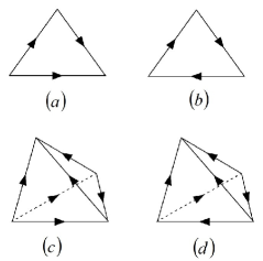
Figure 22: Examples of allowed ((a),(c)) and unallowed ((b),(d)) branching for a $2$-simplex and a $3$-simplex.

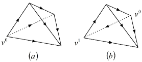
Figure 23: (a): If a $3$-simplex contains a vertex with no incoming edge, we can label this vertex as $v^{0}$ and canonically label the vertices of the remaining $2$-simplex as $v^{1},v^{2},v^{3}$. Such a scheme can be applied for arbitrary $n$-simplex if $n-1$-simplex has a canonical label. (b): If a $3$-simplex contains no vertex without incoming edge, then there must be a vertex with one incoming edge.(Because canonical ordering is true for $2$-simplex.)If we label this vertex as $v^{1}$, the vertex connect to $v^{1}$ through a incoming edge must contain no incoming edge, otherwise the branching rule will be violated. The above argument is true for $n$-simplex if $n-1$ simplex can be canonically ordered.

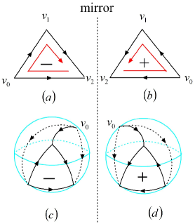
Figure 24: (Color online) (a) and (b): $2$-simplex has two different chiralities, depending on the clockwise or anticlockwise ordering of the vertices. (c) and (d): The chirality of the $3$-simplex can be determined by the chirality of the $2$-simplex which is opposite to the vertex $v^{0}$. Similarly, the chirality of $n$-simplex can be determined by the chirality of $n-1$ simplex which is opposite to $v^{0}$.

A branched $n$-simplex will have the following properties:

(a). Any given branching structure for an $n$-simplex will uniquely determine a canonical ordering of the vertices. For example, Fig. 22 (a) is a branched $2$-simplex with three vertices, one of them contains no incoming edges, one of them contains one incoming edge and the rest of them contains two incoming edges. Thus, we can canonically identify the vertex corresponding to each $v^{i}$, $i=0,1,2$. Such a canonical labeling scheme can be applied to any $n$-simplex, due to the fact that the $n+1$ vertices of any $n$-simplex will be uniquely associated with $0,1,2,\cdots,n$ incoming edges.

Proof.

Assuming the above statement is true for an $n$-simplex (The statement is true when $n=2$, see Fig. 22.), let us prove it is also true for $(n+1)$-simplex. See Fig. 23, if the $(n+1)$-simplex contains a vertex with no incoming edge, we can drop this vertex and apply the statement for the remaining $n$-simplex. If we label the $n+1$ vertices of the $n$-simplex as $1,2,\cdots,n+1$, it is clear the vertex with no incoming edge can be labeled as $0$. In the following we will prove a branched $(n+1)$-simplex must contain a vertex with no incoming edge. If an $(n+1)$-simplex does not contain any vertex with no incoming edge, it must contain a vertex $v^{1}$ with one incoming edge. This is because if we remove an arbitrary vertex (denoted as $v_{0}$) of the $n+1$-simplex, the statement is true for the rest $n$-simplex. Hence we can always find a vertex with one incoming edge. Let us denote this vertex as $v^{1}$ and it is clear that the orientation of the edge that connects $v^{0},v^{1}$ must be outgoing towards $v^{0}$(Otherwise $v^{1}$ is a vertex with no incoming edge). However, in this case, the edges that connect $v^{0}$ and other vertices must be outgoing from $v^{0}$, if the branching rule is not violated. Thus, $v^{0}$ is the vertex with no incoming edge. ∎

(b) Although the branching rule of $n$-simplex uniquely determines the ordering of the vertices, it could not uniquely determine an $n$-simplex. This is simply because the mirror image of a branched $n$-simplex is also a branched $n$-simplex with the same vertices ordering. Thus, any branched $n$-simplex has a unique chirality $\pm 1$.

Proof.

It is clear that $2$-simplex has two different chiralities (see Fig. 24). Assuming that an $n-1$-simplex has a unique chirality, let us deform the boundary of an $n$-simplex (which can be divided into $n-1$-simplex) into an $n-1$ sphere. Due to the fact that there is one and only one vertex $v^{0}$ of an $n$-simplex without incoming edges, we can make a canonical convention and determine the chirality of the $n$ simplex by the chirality of the $n-1$ simplex opposite to $v^{0}$. Such a definition is sufficient because mirror reflection will always change the chirality of the boundary of any $n$-simplex. Indeed, we can define the chirality of the $n$ simplex by the chirality of the $n-1$ simplex opposite to any $v^{i}$ up to a global sign ambiguity (e.g., reversing the chiralities for all $n$-simplices.). ∎

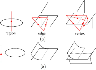
Figure 25: (Color online) (a): Dual representation of branched tetrahedron. (b): We can always induce a smooth structure on oriented manifold from the branched polyhedron. The arrow on the left denotes the orientation of the regions, which is locally identical to their orientations in (a).

The above two properties allow us to use the branched $n$ simplex to represent an $n$-cocycle:

$$\nu_{n}^{s_{ij\ldots k}}(g_{i},g_{j},\cdots,g_{k}),$$ (139)

where $s_{ij\ldots k}=\pm 1$ are determined by the chirality of the simplex and $g_{i},g_{j},\cdots,g_{k}$ are defined on the canonically ordered vertices $v^{0},v^{1},\cdots,v^{n}$.

Finally, let us briefly mention the geometric meaning of the branched tetrahedron in $3$ dimensions. See in Fig. 25 (a), in a dual picture, the orientations of the edges of tetrahedron correspond to the orientations of the region of the simple polyhedron. A branching on a simple polyhedron allows us to smoothen its singularities and equip it with a smooth structure as shown in Fig. 25 (b). At a more rough level, it can be shown that branched tetrahedron can be used to represent the Spin^c-structures on the ambient manifoldsC0527 .

E.2 Basic moves

To show the topological invariance of the amplitude:

$$Z=\frac{\sum_{\{g_{i}\}}}{|G|^{N_{v}}}\prod\nu_{n}^{s_{ij\ldots k}}(g_{i},g_{j},\cdots,g_{k}),$$ (140)

we need to generalize the Turaev-Viro moves to their branched versions in arbitrary dimensions. Because each move will have many different branched versions, it is not easy to check all the branched versions case by case. In the following, we will introduce a simple way to look at the basic moves.

E.2.1 Graphic representation of $(\hskip 1.0pt\mathrm{d}_{n}\nu_{n})(g_{0},g_{1},\cdots,g_{n+1})$ and basic moves

In last section we have shown a branched $n$-simplex can represent an $n$-cocycle $\nu_{n}(g_{i},g_{j},\cdots,g_{k})$ or its inverse $v_{n}^{-1}(g_{i},g_{j},\cdots,g_{k})$, depending on the chirality of the branched $n$-simplex. Here we want to show the boundary of a branched $n+1$-simplex can represent $(\hskip 1.0pt\mathrm{d}_{n}\nu_{n})(g_{0},g_{1},\cdots,g_{n+1})=\prod_{i=0}^{n}\nu_{n}^{(-1)^{i}}(g_{0},\cdots,g_{i-1},g_{i+1},\cdots,g_{n+1})$. Since any $n+1$-simplex branched simplex has a canonical ordering for its $n+2$ vertices and its boundary contains $n+1$ $n$-simplices (We can label these $n+1$ $n$-simplices as $S_{n}(v_{i})$, where $v_{i}$ is the vertex opposite to the $n$-simplex.), it is not surprising if we use the $n$-simplex $S_{n}(v_{i})$ to represent $\nu_{n}(g_{0},\cdots,g_{i-1},g_{i+1},\cdots,g_{n+1})$ or its inverse. However, the key difficulty is that we need to show that the chirality of the $n$-simplex $S_{n}(v_{i})$ is determined by $\pm(-1)^{i}$, where the global sign $\pm$ depends on the chirality of the $n+1$-simplex.

Proof.

It is easy to check that the above statement is true for $n=2$. Thus, we can represent $(\hskip 1.0pt\mathrm{d}_{2}\nu_{2})(g_{0},g_{1},g_{2},g_{3})$ as a branched tetrahedron. Its boundary $2$-simplex $S_{2}(v^{i})$ has opposite chirality for even and odd $i$. If we assume the above statement is true for $n-1$, let us proof it is also true for $n$. First let us remove the vertex $v^{0}$ from the $n+1$-simplex that represents $(\hskip 1.0pt\mathrm{d}_{n}\nu_{n})(g_{0},g_{1},\cdots,g_{n+1})$. By applying the statement to the rest $n$-simplex, whose boundary contains $n$ $n-1$-simplices $S_{n-1}(v^{i})$ ($i=1,2,\cdots,n$) with chirality $\pm(-1)^{i}$. However, according to the definition, the chirality of any $S_{n}(v^{i})$ ($i=1,2,\cdots,n$) can be defined by the $S_{n-1}(v^{i})$ simplex which is opposite to $v^{0}$, thus we prove $S_{n}(v^{i})$ ($i=1,2,\cdots,n$) will also have opposite chiralities for even and odd $i$. To prove that the above statement is also true for $S_{n}(v^{0})$, we can remove any vertex $j\neq 0$ and apply the same scheme. Although there can be a global sign ambiguity for the chirality of any $n$-simplex $S_{n}(v^{i})$ with $i\neq j$, it is sufficient to show $S_{n}(v^{i})$ ($i=0,1,\cdots,n$) will have opposite chiralities for even and odd $i$. Thus, $S_{n}(v^{i})$ ($i=0,1,\cdots,n$) will have chirality $\pm(-1)^{i}$ with the global sign $\pm$ determined by the chirality of the $n+1$-simplex. ∎

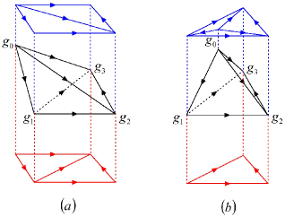
Figure 26: (Color online) $(\hskip 1.0pt\mathrm{d}_{2}\nu_{2})(g_{0},g_{1},g_{2},g_{3})$ can be represented as the boundary of a $3$-simplex. (a) and (b) correspond to two different basic moves of $2$-simplexes.

Based on graphic representation of $(\hskip 1.0pt\mathrm{d}_{n}\nu_{n})(g_{0},g_{1},\cdots,g_{n+1})$, it is easy to check that all the basic moves are actually induced by the identity:

$$\prod_{i=0}^{n}\nu_{n}^{(-1)^{i}}(g_{0},\cdots,g_{i-1},g_{i+1},\cdots,g_{n+1})\equiv 1$$ (141)

Due to this identity, the chirality of the $n+1$-simplex is not important because if we inverse both sides we will end up with the same identity. Thus, we can pick up any $n+1$-simplex to represent $(\hskip 1.0pt\mathrm{d}_{n}\nu_{n})(g_{0},g_{1},\cdots,g_{n+1})$ and project it into the $n$-plane from opposite directions. The shadows of these two projections are $n$-manifold with exact the same vertices. However, they may correspond to different ways of triangulations. Thus, each side of the equations of the basic moves will correspond to the two different ways of projection. For example, Fig. 26 (a) represents $2\leftrightarrow 2$ moves:

$$\nu_{2}(g_{0},g_{1},g_{3})\nu_{2}(g_{1},g_{2},g_{3})=\nu_{2}(g_{0},g_{1},g_{2})\nu_{2}(g_{0},g_{2},g_{3})$$ (142)

and Fig. 26 represents $1\leftrightarrow 3$:

$$\nu_{2}(g_{1},g_{2},g_{3})=\nu_{2}(g_{0},g_{1},g_{2})\nu_{2}(g_{0},g_{2},g_{3})\nu_{2}^{-1}(g_{0},g_{1},g_{3})$$ (143)

However, all these two equations will be equivalent to the identity:

$$\nu_{2}(g_{1},g_{2},g_{3})\nu_{2}^{-1}(g_{0},g_{2},g_{3})\nu_{2}(g_{0},g_{1},g_{3})^{-1}\nu_{2}(g_{0},g_{1},g_{2})\equiv 1$$ (144)

We also notice the projection from opposite directions will induce opposite chiralities for the boundary of the $3$-simplex, that’s why we need to change the chiralities of the $2$-simplex in one side of basic moves. Such a change corresponds to inverse $\nu_{2}$ when we move it from left side to right side of Eq. (141), which is consistent with multiplication rules of the complex number $\nu_{2}$. It is also clear that the above two different moves correspond to projections in different ways, hence all of them are equivalent to the above identity. Similar argument is true for arbitrary dimensions. In conclusion, the identity Eq. (141) will induce the correct $2\leftrightarrow n$ and $1\leftrightarrow n+1$ moves in $n$ dimensions.

E.2.2 Some final details

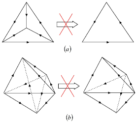
Figure 27: (Color online) Examples of unallowed branched moves in $2$D and $3$D.

It looks like we have successfully generalized the basic moves to their branched versions, however, there are still some subtle issues here, especially in $2$D and $3$D. This is because the $n+1$-simplex representation of the basic moves relies on the assumption that any basic moves can be associated with a consistent branching structure, which is not generically true in $2$D and $3$D. Fig. 27 (a) is an example of unallowed $3\rightarrow 1$ move in $2$D and (b) is an example of unallowed $3\rightarrow 2$ move in $3$D. Although a global labeling scheme will not allow triangulations to contain any local pieces like the left part of Fig. 27, however, those local configurations can be generated during local moves because each simplex still satisfies the branching rule. In this case, we can not directly apply these unallowed local moves to the local pieces. Fortunately, in $2$D and $3$D it has been provedC0527 that any branched triangulations can still be connected through all the allowed moves. In high dimensions, we can show that there are no unallowed moves like these. In the following let us prove this statement.

We notice that the $2\rightarrow n$ move can be realized by adding one more edge while $1\rightarrow n+1$ move can be realized by adding one more vertex and $n+1$ edges, let us show that these two moves are always allowed, by adding proper orientation(s) on the edge(s).

Proof.

It is trivial to show that the $1\rightarrow n+1$ move is always allowed, by adding vertex without incoming edge. The existence of $2\rightarrow n$ move can be slightly more complicated. One can easily check that it is true when $n=2$. Let us assume that it is true for $n-1$-simplex now. We label the two unconnected vertices as $v^{a}$, $v^{b}$ and label other vertices as $v^{i}$.(Notice we don’t require $a,b,i$ have an ordering here.) To show there always exist a proper orientation for the edge $ab$, we only need to show that any triangles made by $v^{a}$, $v^{b}$ and $v^{i}$ will not violate the branching rule. If there exists a vertex $v^{i}$ containing two incoming edges from $v^{a},v^{b}$ or containing two outgoing edges towards $v^{a},v^{b}$, we can remove this vertex and apply the statement to the rest $n-1$ simplex. It does not matter what’s the orientation on $ab$, the triangle $abi$ will not violate branching rule. If such a vertex does not exist, we can show that there can be only two cases: either $v^{a}$ contains no incoming edge, $v^{b}$ contains no outgoing edge or the opposite case. In both cases, we can find a proper orientation for the edge $ab$. ∎

The inverse of the above moves, namely, the $n\rightarrow 2$ move can be realized by removing one edge, and the $n+1\rightarrow 1$ move can be realized by removing one vertex. Now let us show that these moves are always possible when $n>3$.

Proof.

To prove that these moves are always possible in dimensions $n>3$, let us understand why sometimes they are impossible in $2$D and $3$D. Actually, this is simply because three edges of an oriented triangle which violates the branching rule can belong to three different simplices before we apply $3\rightarrow 1$ or $3\rightarrow 2$ move. However, after we apply the move, they belong to the same triangle and hence violate the branching rule. In high dimensions, when we apply these inverse move, we always start from a complete graph and the number of simplices is always larger than $3$. Thus, any triangle must belong to one of the $n$-simplex and will not violating the branching rule. If there is no triangle violate the branching rule in a complete graph, of course there will be no triangle violating the branching rule by removing edge or vertex. ∎

Appendix F (1+1)D solutions of eqn. (12)

F.1 $U^{i}(g)$ is a linear representation

To show that $U^{\bm{i}}(g)$ defined in eqn. (27) is a linear representation of $G$, let us compare the combined actions of $U^{\bm{i}}(g)$ and $U^{\bm{i}}(g^{\prime}g^{-1})$ with the action of $U^{\bm{i}}(g^{\prime})$ which are given by (see Fig. 28)

$$\ \ \ \ U^{\bm{i}}(g^{\prime}g^{-1})U^{\bm{i}}(g)|\alpha_{1},\alpha_{2}\rangle$$ (145)

$$=f_{2}(\alpha_{1},\alpha_{2},g,g^{*})f_{2}(g\alpha_{1},g\alpha_{2},g^{\prime}g^{-1},g^{*})|g^{\prime}\alpha_{1},g^{\prime}\alpha_{2}\rangle$$

and

$$U^{\bm{i}}(g^{\prime})|\alpha_{1},\alpha_{2}\rangle =f_{2}(\alpha_{1},\alpha_{2},g^{\prime},g^{*})|g^{\prime}\alpha_{1},g^{\prime}\alpha_{2}\rangle$$ (146)

We see that

$$\ \ \ \ f_{2}(\alpha_{1},\alpha_{2},g,g^{*})f_{2}(g\alpha_{1},g\alpha_{2},g^{\prime}g^{-1},g^{*})f_{2}^{-1}(\alpha_{1},\alpha_{2},g^{\prime},g^{*})$$

$$=\frac{\nu_{2}(\alpha_{1},g^{-1}g^{*},g^{*})}{\nu_{2}(\alpha_{2},g^{-1}g^{*},g^{*})}\frac{\nu_{2}(g\alpha_{1},gg^{\prime-1}g^{*},g^{*})}{\nu_{2}(g\alpha_{2},gg^{\prime-1}g^{*},g^{*})}\frac{\nu_{2}(\alpha_{2},g^{\prime-1}g^{*},g^{*})}{\nu_{2}(\alpha_{1},g^{\prime-1}g^{*},g^{*})}$$

$$=\frac{\nu_{2}(\alpha_{1},g^{-1}g^{*},g^{*})}{\nu_{2}(\alpha_{2},g^{-1}g^{*},g^{*})}\frac{\nu_{2}(\alpha_{1},g^{\prime-1}g^{*},g^{-1}g^{*})}{\nu_{2}(\alpha_{2},g^{\prime-1}g^{*},g^{-1}g^{*})}\frac{\nu_{2}(\alpha_{2},g^{\prime-1}g^{*},g^{*})}{\nu_{2}(\alpha_{1},g^{\prime-1}g^{*},g^{*})}$$ (147)

The above expression can be represented as Fig. 28 which indicates that the expression is equal to 1. Thus $U^{\bm{i}}(g)$ defined in eqn. (26) form a unitary representation of $G$.

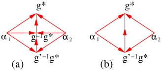
Figure 28: (Color online) The evaluation of the 2-cocycle $\nu_{2}$ on the above two complexes with branching structure gives rise to two phase factors in eqn. (145) and eqn. (146), which shows that the ratio of the two factors, eqn. (F.1), is equal to 1, since the complexes in (a) and (b) overlap.

F.2 $U^{i}(g)$ satisfies eqn. (12)

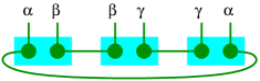
Figure 29: (Color online) The 1D state eqn. (VI.2) on a ring. The degrees of freedom form maximally entangled dimer states.

The action of $\otimes U^{\bm{i}}(g)$ on the 1D state on a ring in Fig. 29 is given by

$$\ \ \ \otimes_{\bm{i}}U^{\bm{i}}(g)|\alpha,\beta;\beta,\gamma;\gamma,\alpha\rangle$$ (148)

$$=f_{2}(\alpha,\beta,g,g^{*})f_{2}(\beta,\gamma,g,g^{*})f_{2}(\gamma,\alpha,g,g^{*})\times$$

$$\ \ \ \ \ |g\alpha,g\beta;g\beta,g\gamma;g\gamma,g\alpha\rangle.$$

From (27), we see that

$$\ \ \ \ f_{2}(\alpha,\beta,g,g^{*})f_{2}(\beta,\gamma,g,g^{*})f_{2}(\gamma,\alpha,g,g^{*})$$

$$=\frac{\nu_{2}(\alpha,g^{-1}g^{*},g^{*})}{\nu_{2}(\beta,g^{-1}g^{*},g^{*})}\frac{\nu_{2}(\beta,g^{-1}g^{*},g^{*})}{\nu_{2}(\gamma,g^{-1}g^{*},g^{*})}\frac{\nu_{2}(\gamma,g^{-1}g^{*},g^{*})}{\nu_{2}(\alpha,g^{-1}g^{*},g^{*})}$$

$$=1$$ (149)

We find that

$$\otimes_{\bm{i}}U^{\bm{i}}(g)|\alpha,\beta;\beta,\gamma;\gamma,\alpha\rangle=|g\alpha,g\beta;g\beta,g\gamma;g\gamma,g\alpha\rangle.$$

The state $|\Psi_{\text{pSRE}}\rangle$ on a ring is invariant under the symmetry transformation. So, $U^{\bm{i}}$ defined in eqn. (26) is indeed a solution of eqn. (12). We can obtain one solution for every cocycle in ${\cal H}^{2}(G,U(1))$ and each solution correspond to a SPT phase in $1$ dimensions.

F.3 States at the chain end form a projective representation

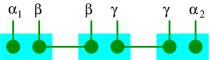
Figure 30: (Color online) A segment of 1D chain with open ends. The degrees of freedom not on the end form maximally entangled dimer states.

Now let us consider the action of on-site symmetry transformation $\otimes_{\bm{i}}U^{\bm{i}}(g)$ on a segment with boundary (see Fig. 30):

$$\ \ \ \otimes_{\bm{i}}U^{\bm{i}}(g)|\alpha_{1},\beta;\beta,\gamma;\gamma,\alpha_{2}\rangle$$ (150)

$$=f_{2}(\alpha_{1},\beta,g,g^{*})f_{2}(\beta,\gamma,g,g^{*})f_{2}(\gamma,\alpha_{2},g,g^{*})\times$$

$$\ \ \ \ \ |g\alpha_{1},g\beta;g\beta,g\gamma;g\gamma,g\alpha_{2}\rangle$$

$$=\frac{\nu_{2}(\alpha_{1},g^{-1}g^{*},g^{*})}{\nu_{2}(\alpha_{2},g^{-1}g^{*},g^{*})}.$$

or

$$\otimes_{\bm{i}}U^{\bm{i}}(g)|\alpha_{1},\alpha_{2}\rangle_{0} =\frac{\nu_{2}(\alpha_{1},g^{-1}g^{*},g^{*})}{\nu_{2}(\alpha_{2},g^{-1}g^{*},g^{*})}|g\alpha_{1},g\alpha_{2}\rangle_{0},$$ (151)

where

$$|\alpha_{1},\alpha_{2}\rangle_{0}=\sum_{\beta,\gamma}|\alpha_{1},\beta;\beta,\gamma;\gamma,\alpha_{2}\rangle.$$ (152)

Eqn. (151), is the same as eqn. (26) and eqn. (27). Thus, $\otimes_{\bm{i}}U^{\bm{i}}(g)$ form a linear representation of $G$.

Note that $|\alpha_{1},\alpha_{2}\rangle_{0}$ is the ground state of our fixed-point model on a segment of chain, where all the internal degrees of freedom form the maximally entangled dimers (just like the ground state on a ring), while the boundary degrees of freedom are labeled by $\alpha_{1}$ and $\alpha_{2}$ on the chain ends. $\alpha_{1}$ and $\alpha_{2}$ label the effective low energy degrees of freedom $|\alpha_{1},\alpha_{2}\rangle_{0}$. Those low energy degrees of freedom form a linear representation of the symmetry transformation as expected. Eqn. (151) describe how the boundary low energy degrees of freedom $|\alpha_{1},\alpha_{2}\rangle_{0}$ transform under the symmetry transformation.

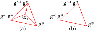
Figure 31: (Color online) (a) The graphic representation of $\frac{\nu_{2}(\alpha_{1},g^{\prime-1}g^{*},g^{-1}g^{*})\nu_{2}(\alpha_{1},g^{-1}g^{*},g^{*})}{\nu_{2}(\alpha_{1},g^{\prime-1}g^{*},g^{*})}$. (b) The graphic representation of $\nu_{2}(g^{\prime-1}g^{*},g^{-1}g^{*},g^{*})$ which allows us to show $\frac{\nu_{2}(\alpha_{1},g^{\prime-1}g^{*},g^{-1}g^{*})\nu_{2}(\alpha_{1},g^{-1}g^{*},g^{*})}{\nu_{2}(\alpha_{1},g^{\prime-1}g^{*},g^{*})}=\nu_{2}(g^{\prime-1}g^{*},g^{-1}g^{*},g^{*})$.

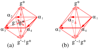
Figure 32: (Color online) (a) The graphic representation of the phase factor eqn. (G.1). (b) The graphic representation of the phase factor eqn. (156). The graphic representations indicate that the two phases are the same.

On the other hand, the symmetry transformation $\otimes_{\bm{i}}U^{\bm{i}}(g)$ factorize (see eqn. (151)), also as expected. This is because the degrees of freedom labeled by $\alpha_{1}$ and $\alpha_{2}$ are located far apart and decouple. We have (on the end whose states are labeled by $\alpha_{1}$)

$$\otimes_{\bm{i}}U^{\bm{i}}(g)|\alpha_{1}\rangle_{0} =\nu_{2}(\alpha_{1},g^{-1}g^{*},g^{*})|g\alpha_{1}\rangle_{0}.$$ (153)

Such transformation satisfies (see Fig. 31)

$$\ \ \ \ \otimes_{\bm{i}}U^{\bm{i}}(g^{\prime}g^{-1})\otimes_{\bm{i}}U^{\bm{i}}(g)|\alpha_{1}\rangle_{0}$$

$$=\frac{\nu_{2}(g\alpha_{1},gg^{\prime-1}g^{*},g^{*})\nu_{2}(\alpha_{1},g^{-1}g^{*},g^{*})}{\nu_{2}(\alpha_{1},g^{\prime-1}g^{*},g^{*})}\otimes_{\bm{i}}U^{\bm{i}}(g^{\prime})|\alpha_{1}\rangle_{0}$$

$$=\frac{\nu_{2}(\alpha_{1},g^{\prime-1}g^{*},g^{-1}g^{*})\nu_{2}(\alpha_{1},g^{-1}g^{*},g^{*})}{\nu_{2}(\alpha_{1},g^{\prime-1}g^{*},g^{*})}\otimes_{\bm{i}}U^{\bm{i}}(g^{\prime})|\alpha_{1}\rangle_{0}$$

$$=\nu_{2}(g^{\prime-1}g^{*},g^{-1}g^{*},g^{*})\otimes_{\bm{i}}U^{\bm{i}}(g^{\prime})|\alpha_{1}\rangle_{0}.$$ (154)

We see that the degrees of freedom on one end form a projective representation labeled by the 2-cocycle $\nu_{2}$, the same 2-cocycle $\nu_{2}$ that characterize the symmetry transformation of the SRE state.

Appendix G (2+1)D solutions of eqn. (12)

G.1 $U^{i}(g)$ is a linear representation

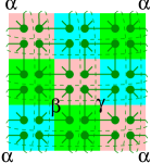
Figure 33: (Color online) A 2D $|\Psi_{\text{pSRE}}\rangle$ state on a torus. In $|\Psi_{\text{pSRE}}\rangle$, the linked dots carry the same index $\alpha,\beta,\gamma,...$

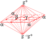
Figure 34: (Color online) The graphic representation of the phase $F_{3}$ in eqn. (157). $F_{3}$ is the value of a 3-cocycle $\nu_{3}$ on the above complex with a branching structure. Note that the top pyramid and the bottom pyramid each form a solid torus (due to the periodic boundary condition) and the whole complex is a sphere. So $F_{3}=1$. Note that the two pyramids on top and blow each small square represent the phase factor $f_{3}$ in eqn. (30).

To show that $U^{\bm{i}}$ defined in eqn. (30) is a linear representation of $G$, let us compare the action of two symmetry transformations: $U^{\bm{i}}(g)U^{\bm{i}}(g^{-1}g^{\prime})$ with the action of $U^{\bm{i}}(g^{\prime})$, which changes $|\alpha_{1},\alpha_{2},\alpha_{3},\alpha_{4}\rangle$ to $|g^{\prime}\alpha_{1},g^{\prime}\alpha_{2},g^{\prime}\alpha_{3},g^{\prime}\alpha_{4}|>$. One has a phase factor

$$\ \ \ \ \frac{\nu_{3}(\alpha_{1},\alpha_{2},g^{-1}g^{*},g^{*})\nu_{3}(\alpha_{2},\alpha_{3},g^{-1}g^{*},g^{*})}{\nu_{3}(\alpha_{4},\alpha_{3},g^{-1}g^{*},g^{*})\nu_{3}(\alpha_{1},\alpha_{4},g^{-1}g^{*},g^{*})}\times$$

$$\ \ \ \ \frac{\nu_{3}(g\alpha_{1},g\alpha_{2},gg^{\prime-1}g^{*},g^{*})\nu_{3}(g\alpha_{2},g\alpha_{3},gg^{\prime-1}g^{*},g^{*})}{\nu_{3}(g\alpha_{4},g\alpha_{3},gg^{\prime-1}g^{*},g^{*})\nu_{3}(g\alpha_{1},g\alpha_{4},gg^{\prime-1}g^{*},g^{*})}$$

$$=\frac{\nu_{3}(\alpha_{1},\alpha_{2},g^{-1}g^{*},g^{*})\nu_{3}(\alpha_{2},\alpha_{3},g^{-1}g^{*},g^{*})}{\nu_{3}(\alpha_{4},\alpha_{3},g^{-1}g^{*},g^{*})\nu_{3}(\alpha_{1},\alpha_{4},g^{-1}g^{*},g^{*})}\times$$ (155)

$$\ \ \ \ \frac{\nu_{3}(\alpha_{1},\alpha_{2},g^{\prime-1}g^{*},g^{-1}g^{*})\nu_{3}(\alpha_{2},\alpha_{3},g^{\prime-1}g^{*},g^{-1}g^{*})}{\nu_{3}(\alpha_{4},\alpha_{3},g^{\prime-1}g^{*},g^{-1}g^{*})\nu_{3}(\alpha_{1},\alpha_{4},g^{\prime-1}g^{*},g^{-1}g^{*})}$$

and the other has a phase factor

$$\frac{\nu_{3}(\alpha_{1},\alpha_{2},g^{\prime-1}g^{*},g^{*})\nu_{3}(\alpha_{2},\alpha_{3},g^{\prime-1}g^{*},g^{*})}{\nu_{3}(\alpha_{4},\alpha_{3},g^{\prime-1}g^{*},g^{*})\nu_{3}(\alpha_{1},\alpha_{4},g^{\prime-1}g^{*},g^{*})}$$ (156)

From their graphic representations Fig. 32, we see that the two phases are the same. Thus $U^{\bm{i}}(g)$ form an unitary representation of the symmetry group $G$.

G.2 $U^{i}(g)$ satisfies eqn. (12)

Following a similar approach as for the (1+1)D case, we can also show that the state $|\Psi_{\text{pSRE}}\rangle$ on a 2D complex (see Fig. 33) that is a boundary of another graph is invariant under the symmetry transformation $\otimes_{\bm{i}}U^{\bm{i}}$ (see Fig. 34):

$$\otimes_{\bm{i}}U^{\bm{i}}|\Psi_{\text{pSRE}}\rangle=F_{3}|\Psi_{\text{pSRE}}\rangle=|\Psi_{\text{pSRE}}\rangle$$ (157)

So, $U^{\bm{i}}$ defined in eqn. (30) is indeed a solution of eqn. (12). We can obtain one solution for every cocycle in ${\cal H}^{3}(G,U_{T}(1))$ and each solution correspond to a SPT phase in $2$ dimensions.

G.3 The action of $\otimes U^{i}(g)$ on $|\Psi_{\text{pSRE}}\rangle$ with boundary

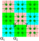
Figure 35: (Color online) A 2D $|\Psi_{\text{pSRE}}\rangle$ state on an open square. In $|\Psi_{\text{pSRE}}\rangle$, the linked dots carry the same index $\alpha_{1},\alpha_{2},\beta,\gamma,...$ The indices on the boundary are given by $\alpha_{1},\alpha_{2},...$ The indices inside the square are given by $\beta,\gamma,...$

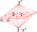
Figure 36: (Color online) The graphic representation of the phase $\tilde{F}_{3}(g,g^{*};\alpha_{1},\alpha_{2},\beta,\gamma,...)$ in eqn. (G.3). Compare to the complex in Fig. 34, the above complex do not have the periodic boundary condition.

Now let us consider the action of $\otimes_{\bm{i}}U^{\bm{i}}$ on a state in Fig. 35 with a boundary (see Fig. 36):

$$\ \ \ \ \otimes_{\bm{i}}U^{\bm{i}}(g)|\alpha_{1},\alpha_{2},\beta,\gamma,...\rangle$$

$$=\tilde{F}_{3}(g,g^{*};\alpha_{1},\alpha_{2},\beta,\gamma,...)|g\alpha_{1},g\alpha_{2},g\beta,g\gamma,...\rangle$$ (158)

From the Fig. 36 and the geometric meaning of the cocycles, we find that

$$\tilde{F}_{3}(g,g^{*};\alpha_{1},\alpha_{2},\beta,\gamma,...)=\prod_{\langle ij\rangle}\nu^{s_{ij}}_{3}(\alpha_{i},\alpha_{j},g^{-1}g^{*},g^{*})$$ (159)

where $\prod_{\langle ij\rangle}$ is a product over the nearest neighbor bonds $\{ij\}$, $|i-j|=1$, around the boundary. The direction $i\to j$ is the direction of the bond and $s_{ij}=1$ f $i>j$, $s_{ij}=-1$ f $i<j$. Since $\tilde{F}_{3}$ is independent of the indices $\beta,\gamma,...$ that are not on the boundary, we find

$$\ \ \ \ \otimes_{\bm{i}}U^{\bm{i}}(g)|\{\alpha_{i}\}\rangle_{0}=\prod_{\langle ij\rangle}\nu^{s_{ij}}_{3}(\alpha_{i},\alpha_{j},g^{-1}g^{*},g^{*})|\{g\alpha_{i}\}\rangle_{0}$$ (160)

where $|\{\alpha_{i}\}\rangle_{0}$ is the SPT state with a boundary which depends on the indices $\{\alpha_{i}\}$ on the boundary:

$$|\{\alpha_{i}\}\rangle_{0}=\sum_{\beta,\gamma,...\in G}|\alpha_{1},\alpha_{2},\beta,\gamma,...\rangle.$$ (161)

We see that the action of $\otimes_{\bm{i}}U^{\bm{i}}(g)$ on $|\{\alpha_{i}\}\rangle_{0}$ is very similar to the action of a single $U^{\bm{i}}(g)$ on a single site (compare Figs. 12 and 36). Using a similar approach, we can show that $\otimes_{\bm{i}}U^{\bm{i}}(g)$ indeed form a linear representation (see Fig. 32), when viewed as an operator $U_{b}(g)$ acting on the boundary state $|\{\alpha_{i}\}\rangle_{0}$.

To summarize, we discussed the form of on-site symmetry transformations $\otimes_{\bm{i}}U^{\bm{i}}(g)$ in a basis where the many-body ground state is a simple product state. We find that different on-site symmetry transformations can be constructed from each 3-cocycle $\nu_{3}$ in ${\cal H}^{3}[G,U_{T}(1)]$.

We would like to stress that, in such a simple basis, the symmetry transformation $\otimes_{\bm{i}}U^{\bm{i}}(g)$ on the boundary (160) has a very unusual locality property: Due to the non-trivial phase factor $\prod_{\langle ij\rangle}\nu^{s_{ij}}_{3}(\alpha_{i},\alpha_{j},g^{-1}g^{*},g^{*})$, we cannot view $U_{b}(g)$ (acting on the boundary state $|\{\alpha_{i}\}\rangle_{0}$) as a direct product of local operators acting on each boundary sites $|\alpha_{i}\rangle$. (Note that we can view the boundary state $|\{\alpha_{i}\}\rangle_{0}$ as $|\{\alpha_{i}\}\rangle_{0}=\otimes_{i\in\text{boundary}}|\alpha_{i}\rangle$.) Therefore, $U_{b}(g)$ is not a on-site symmetry transformation on the boundary.

In the above, we have viewed $i$ as effective sites on the boundary with physical states $|\alpha_{i}\rangle$ on each site. We see that the symmetry transformation is not an on-site symmetry transformation. If we view, instead, each nearest neighbor bond $\langle ij\rangle$ as an effective site with physical states $|\alpha_{i}\alpha_{j}\rangle$ on each site, then the symmetry transformation will be an “on-site” symmetry transformation, but the states on different bounds are not independent and $|\{\alpha_{i}\}\rangle_{0}\neq\otimes_{\langle ij\rangle\in\text{boundary}}|\alpha_{i}\alpha_{j}\rangle$.

Thus in a basis where the many-body ground state is a simple product state, although $\otimes_{\bm{i}}U^{\bm{i}}(g)$ is an on-site symmetry transformation when acting on the bulk state, it cannot be an on-site symmetry transformation when viewed as a symmetry transformation acting on the effective low energy degrees of freedom on the boundary when the 3-cocycle $\nu_{3}$ is non-trivial. This is the non-trivial physical properties that characterize a non-trivial SPT phase in (2+1)D (see appendix I and LABEL:CLW1152 for more details).

Appendix H Two symmetry representations in our fixed-point model

In the old basis in the path integral formalism [see eqn. (54)], the wave function is complicated, but the many-body on-site symmetry transformation has the following locality structure

$$\otimes_{i}U^{i}(g)$$ (162)

where $U^{i}(g)$ is the symmetry transformation on the $i^{th}$ site

$$U^{i}(g)|g_{i}\rangle=|gg_{i}\rangle.$$ (163)

This is the definition of the so called on-site symmetry transformation.

In the new basis[see eqn. (56)], the wave function is simple but the many-body symmetry transformation is no longer an on-site symmetry transformation. It has the following form

$$\ \ \ \ \otimes_{i}U^{i}(g)|\{g_{i}\}_{M}\rangle^{\prime}$$

$$=\frac{\prod_{\{ij...*\}}\nu_{1+d}^{s_{ij...*}}(g_{i},g_{j},...,g^{*})}{\prod_{\{ij...*\}}\nu_{1+d}^{s_{ij...*}}(gg_{i},gg_{j},...,g^{*})}|\{gg_{i}\}_{M}\rangle^{\prime}$$

$$=\frac{\prod_{\{ij...*\}}\nu_{1+d}^{s_{ij...*}}(g_{i},g_{j},...,g^{*})}{\prod_{\{ij...*\}}\nu_{1+d}^{s_{ij...*}}(g_{i},g_{j},...,g^{-1}g^{*})}|\{gg_{i}\}_{M}\rangle^{\prime}$$

$$=|\{gg_{i}\}_{M}\rangle^{\prime}$$ (164)

where $U^{i}(g)$ is the symmetry transformation that acts on the $i^{th}$ and $(i\pm 1)^{th}$ sites [in (1+1)D for example]

$$U^{i}(g)|g_{i-1},g_{i},g_{i+1}\rangle^{\prime}=f_{2}(g_{i-1},g_{i},g_{i+1},g)|g_{i-1},gg_{i},g_{i+1}\rangle^{\prime}.$$ (165)

Here the phase factor $f_{2}$ is given by the 2-cocycles

$$\ \ \ \ f_{2}(g_{i-1},g_{i},g_{i+1},g)$$

$$=\frac{\nu_{2}(g_{i-1},g_{i},g^{*})\nu_{2}(g_{i},g_{i+1},g^{*})}{\nu_{2}(g_{i-1},gg_{i},g^{*})\nu_{2}(gg_{i},g_{i+1},g^{*})}$$ (166)

where $g^{*}$ is an fixed element in $G$. For example we may choose $g^{*}=1$.

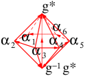
Figure 37: (Color online) The graphic representation of the product of the phase factor $\prod_{\langle ij\rangle}\nu^{s_{ij}}_{3}(\alpha_{i},\alpha_{j},g^{-1}g^{*},g^{*})$ in eqn. (160).

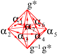
Figure 38: (Color online) The graphic representation of the product of the phase factor $\frac{\prod_{\{ij...*\}}\nu_{1+d}^{s_{ij...*}}(\alpha_{i},\alpha_{j},...,g^{*})}{\prod_{\{ij...*\}}\nu_{1+d}^{s_{ij...*}}(\alpha_{i},\alpha_{j},...,g^{-1}g^{*})}$ in eqn. (H) for a 2D complex $(\alpha_{1},...,\alpha_{7})$ with a boundary $(\alpha_{1},...,\alpha_{6})$.

We have seen that, in the new basis, we still have $\otimes_{i}U^{i}(g)|\{g_{i}\}_{M}\rangle^{\prime}=|\{gg_{i}\}_{M}\rangle^{\prime}$ if the state $|\{g_{i}\}_{M}\rangle^{\prime}$ is defined on a complex $M$ which is the boundary of another complex $M_{\text{ext}}$. It is hard to see the non on-site structure of $\otimes_{i}U^{i}(g)$. To expose the non on-site structure of $\otimes_{i}U^{i}(g)$ in the new basis, let us consider the action of $\otimes_{i}U^{i}(g)$ on a state defined on a complex that has a boundary. In this case, we still have

$$\ \ \ \ \otimes_{i}U^{i}(g)|\{g_{i}\}_{M}\rangle^{\prime}$$

$$=\frac{\prod_{\{ij...*\}}\nu_{1+d}^{s_{ij...*}}(g_{i},g_{j},...,g^{*})}{\prod_{\{ij...*\}}\nu_{1+d}^{s_{ij...*}}(g_{i},g_{j},...,g^{-1}g^{*})}|\{gg_{i}\}_{M}\rangle^{\prime}$$ (167)

But now, the phase factor is not equal to 1.

In Fig. 38, we give a graphic representation of the above phase factor $\frac{\prod_{\{ij...*\}}\nu_{1+d}^{s_{ij...*}}(\alpha_{i},\alpha_{j},...,g^{*})}{\prod_{\{ij...*\}}\nu_{1+d}^{s_{ij...*}}(\alpha_{i},\alpha_{j},...,g^{-1}g^{*})}$ for a 2D complex with a boundary. We see that the complex in Fig. 38 and Fig. 37 have the same surface. So the phase factor represented by Fig. 38 equal to that represented by Fig. 37. So eqn. (160) is the same as eqn. (H).

We have discussed two ways to classify SPT phases. The first way to classify SPT phases is to classify symmetry transformations that act on simple wave function $|\Psi_{\text{pSRE}}\rangle$, which lead to eqn. (160). The second way to classify SPT phases is to classify fixed-point action-amplitude (the topological terms) which lead to eqn. (H). The above analysis indicates that the two ways to classify SPT phases are equivalent.

The equivalence between the two formalisms eqn. (160) and eqn. (H) will become more clear after a duality transformation.

In the following we will show that the ground state wave function (56) in the Lagrangian formalism is dual to the ground state wave function (VI.2) in the Hamiltonian formalism discussed in Sec. IV and V. Furthermore, after the duality transformation, the the symmetry representations (55) are the same as that defined in eqn. (26) or eqn. (160).

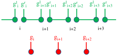
Figure 39: (Color online) The dual transformation in the new bases in 1D.

Let us illustrate the above result in 1D. Firstly, we introduce the dual transformation which maps a state to its dual wave function living on the dual lattice. In the dual transformation, the bases $|g_{i}\rangle$ at site $i$ correspond to the bond $|g_{i}^{r},g_{i+1}^{l}\rangle$ in the dual lattice (see Fig. 39), where $g_{i}^{r}=g_{i+1}^{l}=g_{i}$ and the amplitude of the configuration remains unchanged. In this way, we obtain the dual wave function $\Psi_{d}(\{g_{i}^{l},g_{i}^{r}\})$ of $\Psi(\{g_{i}\})$.

Now we introduce the new bases $|\{g_{i}^{l},g_{i}^{r}\}\rangle^{\prime}$ through the LU transformation introduced in eqn. (56),

$$|\{g_{i}^{l},g_{i}^{r}\}\rangle^{\prime} = \prod_{i}\nu_{2}(g_{i},g_{i+1},g^{*})|\{g_{i}^{l},g_{i}^{r}\}\rangle$$ (168)

$$= \prod_{i}\nu_{2}(g_{i}^{r},g_{i+1}^{r},g^{*})|\{g_{i}^{l},g_{i}^{r}\}\rangle$$

$$= \prod_{i}\left[\nu_{2}(g_{i+1}^{l},g_{i+1}^{r},g^{*})|{g_{i+1}^{l},g_{i+1}^{r}}\rangle\right]$$

In the new bases, the fixed point state in the dual lattice becomes a direct product of bonds. Notice that the previous local unitary transformation in eqn. (56) becomes on-site unitary transformation. Furthermore, in the new bases the symmetry representation also becomes on-site and is fractionalized into two ‘projective’ operations:

$$\otimes_{i}U^{i}(g)|\{g_{i}^{l},g_{i}^{r}\}\rangle^{\prime}$$ (169)

$$= \prod_{i}\nu_{2}(g_{i+1}^{l},g_{i+1}^{r},g^{*})|\{gg_{i+1}^{l},gg_{i+1}^{r}\}\rangle$$

$$= \prod_{i}\frac{\nu_{2}(g_{i+1}^{l},g_{i+1}^{r},g^{*})}{\nu_{2}(g_{i+1}^{l},g_{i+1}^{l},g^{-1}g^{*})}|\{gg_{i+1}^{l},gg_{i+1}^{r}\}\rangle^{\prime}$$

$$= \prod_{i}\frac{\nu_{2}(g_{i+1}^{l},g^{-1}g^{*},g^{*})}{\nu_{2}(g_{i+1}^{r},g^{-1}g^{*},g^{*})}|\{gg_{i+1}^{l},gg_{i+1}^{r}\}\rangle^{\prime}$$

Above formula is the same as eqn. (27).

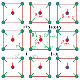
Figure 40: (Color online) The duality transformation in 2-dimension. The green dots represent the dual lattice of the red dots. In the new bases, the wave function in the green lattice is the same as the one introduced in Sec. III and IV.

Similarly, we can illustrate the result in 2D. Now the basis $|g_{i}\rangle$ correspond to $|g_{i}^{1},g_{i+x}^{2},g_{i+x+y}^{3},g_{i+y}^{4}\rangle$ in the dual lattice (see Fig. 40). After the dual transformation, the wave function $\Psi(\{g_{i}\})$ becomes $\Psi_{d}(\{g_{i}^{1},g_{i}^{2},g_{i}^{3},g_{i}^{4}\})$ (here $g_{i}^{1}=g_{i+x}^{2}=g_{i+x+y}^{3}=g_{i+y}^{4}=g_{i}$). Again, we introduce the LU transformation

$$|\{g_{i}^{1},g_{i}^{2},g_{i}^{3},g_{i}^{4}\}\rangle^{\prime}$$ (170)

$$= \prod_{i}\frac{\nu_{3}(g_{i},g_{i+x},g_{i+y},g^{*})}{\nu_{3}(g_{i+x},g_{i+y},g_{\tilde{i}},g^{*})}|\{g_{i}^{1},g_{i}^{2},g_{i}^{3},g_{i}^{4}\}\rangle$$

$$= \prod_{i}\frac{\nu_{3}(g_{\tilde{i}}^{3},g_{\tilde{i}}^{4},g_{\tilde{i}}^{2},g^{*})}{\nu_{3}(g_{\tilde{i}}^{4},g_{\tilde{i}}^{2},g_{\tilde{i}}^{1},g^{*})}|\{g_{\tilde{i}}^{1},g_{\tilde{i}}^{2},g_{\tilde{i}}^{3},g_{\tilde{i}}^{4}\}\rangle$$

where $\tilde{i}=i+x+y$. The LU transformation between the old bases and the new ones is an on-site. In the new bases, the fixed point wave function is a direct product of plaquettes. The symmetry operation now becomes

$$\otimes_{i}U^{i}(g)|\{g_{i}^{1},g_{i}^{2},g_{i}^{3},g_{i}^{4}\}\rangle^{\prime}$$ (171)

$$= \prod_{i}\frac{\nu_{3}(g_{\tilde{i}}^{3},g_{\tilde{i}}^{4},g_{\tilde{i}}^{2},g^{*})}{\nu_{3}(g_{\tilde{i}}^{4},g_{\tilde{i}}^{2},g_{\tilde{i}}^{1},g^{*})}|\{gg_{\tilde{i}}^{1},gg_{\tilde{i}}^{2},gg_{\tilde{i}}^{3},gg_{\tilde{i}}^{4}\}\rangle$$

$$= \prod_{i}\frac{\nu_{3}(g_{\tilde{i}}^{3},g_{\tilde{i}}^{4},g_{\tilde{i}}^{2},g^{*})}{\nu_{3}(g_{\tilde{i}}^{4},g_{\tilde{i}}^{2},g_{\tilde{i}}^{1},g^{*})}\prod_{i}\frac{\nu_{3}(g_{\tilde{i}}^{4},g_{\tilde{i}}^{2},g_{\tilde{i}}^{1},g^{-1}g^{*})}{\nu_{3}(g_{\tilde{i}}^{3},g_{\tilde{i}}^{4},g_{\tilde{i}}^{2},g^{-1}g^{*})}$$

$$\times|\{gg_{\tilde{i}}^{1},gg_{\tilde{i}}^{2},gg_{\tilde{i}}^{3},gg_{\tilde{i}}^{4}\}\rangle^{\prime}$$

$$= \prod_{i}\frac{\nu_{3}(g_{\tilde{i}}^{3},g_{\tilde{i}}^{4},g^{-1}g^{*},g^{*})\nu_{3}(g_{\tilde{i}}^{4},g_{\tilde{i}}^{1},g^{-1}g^{*},g^{*})}{\nu_{3}(g_{\tilde{i}}^{3},g_{\tilde{i}}^{2},g^{-1}g^{*},g^{*})\nu_{3}(g_{\tilde{i}}^{2},g_{\tilde{i}}^{1},g^{-1}g^{*},g^{*})}$$

$$\times|\{gg_{\tilde{i}}^{1},gg_{\tilde{i}}^{2},gg_{\tilde{i}}^{3},gg_{\tilde{i}}^{4}\}\rangle^{\prime}$$

Above equation agree with eqn. (VI.3).

From the above examples, we can see that after the ‘dual transformation’ the ground state wave function and its symmetry representation in the Lagrangian formalism are the same as the Hamiltonian formalism as we discussed in Sec.VI.

Appendix I $(2+1)D$ SPT states constructed from 3-cocycles and matrix product unitary operator

Based on the 3-cocycles $\nu_{3}(g_{0},g_{1},g_{2},g_{3})$ of group $G$, we can construct short range entangled models with SPT order as discussed in section VI.3 (also discussed in appendix G). In order to assess the non trivialness of the SPT order of a certain model, in LABEL:CLW1152 we developed the tool of matrix product unitary operators (MPUO) and used it to show that the particular model we gave in that paper–the CZX model–has very special boundary properties and hence nontrivial SPT order. In this section, we are going to apply the MPUO method to the general models constructed in section VI.3 and show that for the model constructed from a 3-cocycle $\nu_{3}(g_{0},g_{1},g_{2},g_{3})$, the effective MPUO on the boundary transform with the same 3-cocycle. Therefore, according to the result in LABEL:CLW1152, models constructed from nontrivial $\nu_{3}(g_{0},g_{1},g_{2},g_{3})$ must either break the symmetry or have gapless excitations if the system has a boundary. Moreover, we can show the contrary for models constructed from trivial $\nu_{3}(g_{0},g_{1},g_{2},g_{3})$. That is, for models constructed from trivial $\nu_{3}(g_{0},g_{1},g_{2},g_{3})$ we are going to explicitly construct a short range entangled symmetric state for the effective symmetry on the boundary. For basic definition and properties of MPUO, see LABEL:CLW1152.

We consider in this paper models with on-site symmetry of group $G$. SPT order exist in models whose ground states on a closed manifold are short range entangled and symmetric under the on-site symmetry. The ground state is unique and gapped. If the system has boundary, on the other hand, there are low energy effective degrees of freedom are on the boundary. The effective symmetry on the boundary however, may no longer take an on-site form. In general, the effective symmetry on the 1D boundary of a 2D model can be written as a matrix product unitary operator

$$U=\sum_{\{i_{k}\},\{i_{k}^{\prime}\}}{\rm Tr}(T^{i_{1},i^{\prime}_{1}}T^{i_{2},i^{\prime}_{2}}...T^{i_{N},i^{\prime}_{N}})|i^{\prime}_{1}i^{\prime}_{2}...i^{\prime}_{N}\rangle\langle i_{1}i_{2}...i_{N}|$$ (172)

where $i$ and $i^{\prime}$ are input and output physical indices and for fixed $i$ and $i^{\prime}$, $T^{i,i^{\prime}}$ is a matrix.

For the models defined in section VI.3, the effective symmetry $\tilde{U}(g)$ on the boundary takes the form(see appendix G)

$$\tilde{U}(g)|\{\alpha_{i}\}\rangle=\prod_{i,j}\nu_{3}^{s_{ij}}(\alpha_{i},\alpha_{j},g^{-1}g^{*},g^{*})|\{g\alpha_{i}\}\rangle$$ (173)

where $\prod_{ij}$ is a product over the nearest neighbor bonds $\{ij\}$, $|i-j|=1$, around the boundary. The direction $i\to j$ is the direction of the bond and $s_{ij}=1$ if $i>j$, $s_{ij}=-1$ if $i<j$. This symmetry operator on a 1D chain can be expressed as a MPUO. If the bond goes from $\alpha_{i}$ to $\alpha_{i+1}$

$$\begin{array}[]{l}T_{i}^{\alpha_{i},g\alpha_{i}}(g)=\sum_{\alpha_{i+1}}\nu_{3}^{-1}(\alpha_{i},\alpha_{i+1},g^{-1}g^{*},g^{*})|\alpha_{i}\rangle\langle\alpha_{i+1}|\ ,\forall\alpha_{i}\\ \text{other terms are zero}\end{array}$$ (174)

If the bond goes from $\alpha_{i+1}$ to $\alpha_{i}$,

$$\begin{array}[]{l}T_{i}^{\alpha_{i},g\alpha_{i}}(g)=\sum_{\alpha_{i+1}}\nu_{3}(\alpha_{i+1},\alpha_{i},g^{-1}g^{*},g^{*})|\alpha_{i}\rangle\langle\alpha_{i+1}|\ ,\forall\alpha_{i}\\ \text{other terms are zero}\end{array}$$ (175)

Now we compose multiple MPUOs and find their reduction rule. We will see that the reduction rule is related to the same $\nu_{3}$. First, the combination of $T_{i}(g_{2})$ and $T_{i}(g_{1})$ gives (if the bond goes from $\alpha_{i}$ to $\alpha_{i+1}$)

$$\begin{array}[]{l}T_{i}(g_{1},g_{2})^{\alpha_{i},g_{1}g_{2}\alpha_{i}}=\sum_{\alpha_{i+1},\alpha^{\prime}_{i+1}}\nu_{3}^{-1}(\alpha_{i},\alpha_{i+1},g_{2}^{-1}g^{*},g^{*})\\ \nu_{3}^{*s(g_{2})}(g_{2}\alpha_{i},\alpha^{\prime}_{i+1},g_{1}^{-1}g^{*},g^{*})|\alpha_{i},g_{2}\alpha_{i}\rangle\langle\alpha_{i+1},\alpha^{\prime}_{i+1}|\end{array}$$ (176)

This can be reduced to

$$\ \ \ \ T_{i}(g_{1}g_{2})^{\alpha_{i},g_{1}g_{2}\alpha_{i}}$$

$$=\sum_{\alpha_{i+1}}\nu_{3}^{-1}(\alpha_{i},\alpha_{i+1},g_{2}^{-1}g_{1}^{-1}g^{*},g^{*})|\alpha_{i}\rangle\langle\alpha_{i+1}|$$ (177)

by applying the following projection operator to the right side of the matrices

$$\ \ \ \ P^{r}_{g_{1},g_{2}}$$ (178)

$$=\sum_{\alpha_{i+1}}\nu_{3}^{-1}(\alpha_{i+1},g_{2}^{-1}g_{1}^{-1}g^{*},g_{2}^{-1}g^{*},g^{*})|\alpha_{i+1},g_{2}\alpha_{i+1}\rangle\langle\alpha_{i+1}|$$

and the hermitian conjugate of

$$\ \ \ \ P^{l}_{g_{1},g_{2}}$$

$$=\sum_{\alpha_{i}}\nu_{3}^{-1}(\alpha_{i},g_{2}^{-1}g_{1}^{-1}g^{*},g_{2}^{-1}g^{*},g^{*})|\alpha_{i},g_{2}\alpha_{i}\rangle\langle\alpha_{i}|$$ (179)

to the left side of the matrices. This is because,

$$\ \ \ \ \nu_{3}(g_{2}\alpha_{i},g_{2}\alpha_{i+1},g_{1}^{-1}g^{*},g^{*})$$

$$=\nu_{3}^{s(g_{2})}(\alpha_{i},\alpha_{i+1},g_{2}^{-1}g_{1}^{-1}g^{*},g_{2}^{-1}g^{*})$$ (180)

and the 3-cocycle condition of $\nu_{3}$

$$\begin{array}[]{l}\nu_{3}(\alpha_{i},\alpha_{i+1},g_{2}^{-1}g^{*},g^{*})\nu_{3}(\alpha_{i},\alpha_{i+1},g_{2}^{-1}g_{1}^{-1}g^{*},g_{2}^{-1}g^{*})\\ \nu_{3}^{-1}(\alpha_{i},g_{2}^{-1}g_{1}^{-1}g^{*},g_{2}^{-1}g^{*},g^{*})\nu_{3}(\alpha_{i+1},g_{2}^{-1}g_{1}^{-1}g^{*},g_{2}^{-1}g^{*},g^{*})\\ =\nu_{3}(\alpha_{i},\alpha_{i+1},g_{2}^{-1}g_{1}^{-1}g^{*},g^{*})\end{array}$$ (181)

It is easy to check that the same reduction procedure applies when the bond goes from $\alpha_{i+1}$ to $\alpha_{i}$. The above definition of $P^{l}$ and $P^{r}$ has picked a particular gauge choice of phase for $P^{l}$ and $P^{r}$.

Next we consider the combination of three MPUOs and find the corresponding 3-cocycle associated with different ways of combining the three MPUOs into one. If we combine $T(g_{2})$,$T(g_{1})$ first and then combine $T(g_{1}g_{2})$ with $T(g_{3})$, the combined operation of $P_{g_{1},g_{2}}$ and $P_{g_{1}g_{2},g_{3}}$ is (we omit the site label $i$)

$$\ \ \ \ (P_{g_{1},g_{2}}\otimes I)P_{g_{1}g_{2},g_{3}}$$ (182)

$$=\sum_{\alpha}\nu_{3}(\alpha,g_{3}^{-1}g_{2}^{-1}g_{1}^{-1}g^{*},g_{3}^{-1}g_{2}^{-1}g^{*},g_{3}^{-1}g^{*})\times$$

$$\ \ \ \nu_{3}(\alpha,g_{3}^{-1}g_{2}^{-1}g_{1}^{-1}g^{*},g_{3}^{-1}g^{*},g^{*})|\alpha,g_{3}\alpha,g_{2}g_{3}\alpha\rangle\langle\alpha|.$$

On the other hand, if we combine $T(g_{3})$,$T(g_{2})$ first and then combine $T(g_{2}g_{3})$ with $T(g_{1})$, the combined operator of $P_{g_{2},g_{3}}$ and $P_{g_{1},g_{2}g_{3}}$ is

$$\begin{array}[]{l}(I\otimes P_{g_{2},g_{3}})P_{g_{1},g_{2}g_{3}}=\\ \sum_{\alpha}\nu_{3}(\alpha,g_{3}^{-1}g_{2}^{-1}g^{*},g_{3}^{-1}g^{*},g^{*})\times\\ \nu_{3}(\alpha,g_{3}^{-1}g_{2}^{-1}g_{1}^{-1}g^{*},g_{3}^{-1}g_{2}^{-1}g^{*},g^{*})|\alpha,g_{3}\alpha,g_{2}g_{3}\alpha\rangle\langle\alpha|\end{array}$$ (183)

These two differ by a phase factor

$$\nu_{3}(g_{3}^{-1}g_{2}^{-1}g_{1}^{-1}g^{*},g_{3}^{-1}g_{2}^{-1}g^{*},g_{3}^{-1}g^{*},g^{*})$$ (184)

Hence we see that, the reduction procedure of $T$’s is associative up to phase. The phase factor is the same 3-cocycle that we used to construct the model. From the result in LABEL:CLW1152 we know that if $\nu_{3}$ is nontrivial, the model we constructed has a nontrivial boundary which cannot have a gapped symmetric ground state. It must either break the symmetry or be gapless. Therefore, the model constructed with nontrivial 3-cocycles belong to nontrivial SPT phases.

On the other hand, if the model is constructed from a trivial 3-cocycle, the boundary effective symmetry does allow SRE symmetric state. Actually, the SRE symmetric state on the boundary can be constructed explicitly for the models discussed here. If $\nu_{3}$ is trivial, it takes the form of a 3-coboundary

$$\nu_{3}(g_{0},g_{1},g_{2},g_{3})=\frac{\mu_{2}(g_{1},g_{2},g_{3})\mu_{2}(g_{0},g_{1},g_{3})}{\mu_{2}(g_{0},g_{2},g_{3})\mu_{2}(g_{0},g_{1},g_{2})}$$ (185)

where $\mu_{2}$ is an arbitrary 2-cochain. Note that it is not necessarily a cocycle. The effective symmetry on the boundary can hence be written as

$$\begin{array}[]{l}\tilde{U}(g)|\{\alpha_{i}\}\rangle=\\ \prod_{i,j}\left(\frac{\mu_{2}(\alpha_{j},g^{-1}g^{*},g^{*})\mu_{2}(\alpha_{i},\alpha_{j},g^{*})}{\mu_{2}(\alpha_{i},g^{-1}g^{*},g^{*})\mu_{2}(\alpha_{i},\alpha_{j},g^{-1}g^{*})}\right)^{s_{ij}}|\{g\alpha_{i}\}\rangle\end{array}$$ (186)

The $\mu_{2}(\alpha_{i},g^{-1}g^{*},g^{*})$ terms cancel out in the product of phase factors, and the remaining terms can be grouped into two sets $\prod_{ij}\mu_{2}^{s_{ij}}(\alpha_{i},\alpha_{j},g^{*})$ and $\prod_{ij}\mu_{2}^{-s_{ij}}(\alpha_{i},\alpha_{j},g^{-1}g^{*})=\prod_{ij}\mu_{2}^{-s_{ij}s(g)}(g\alpha_{i},g\alpha_{j},g^{*})$. Define $\Theta(g)=\prod_{ij}\sum_{\alpha_{i},\alpha_{j}}\mu_{2}^{s_{ij}}(\alpha_{i},\alpha_{j},g^{*})|\alpha_{i}\alpha_{j}\rangle\langle\alpha_{i}\alpha_{j}|$. $\Theta(g)$ is a product of local unitaries. It is easy to see that

$$\tilde{U}(g)=\Theta^{{\dagger}}(g)\left(\sum_{\{\alpha_{i}\}}|\{g\alpha_{i}\}\rangle\langle\{\alpha_{i}\}|\right)\Theta(g)$$ (187)

(a complex conjugation operation needs to be added if $\tilde{U}(g)$ is anti-unitary). The term in the middle is an on-site operation which permutes the basis. It has a simple symmetric state which is a product state $\otimes_{i}(\sum_{\alpha_{i}}|\alpha_{i}\rangle)$. Therefore $\Theta^{{\dagger}}(g)\otimes_{i}(\sum_{\alpha_{i}}|\alpha_{i}\rangle)$ is a symmetric state of $\tilde{U}(g)$. Because $\otimes_{i}(\sum_{\alpha_{i}}|\alpha_{i}\rangle)$ is a product state and $\Theta^{{\dagger}}(g)$ is a product of local unitaries, this is a short range entangled state. Therefore, we have explicitly constructed a short range entangled symmetric state on the boundary if the model is constructed from a trivial 3-cocycle $\nu_{3}$.

Appendix J Calculations of group cohomology

In the section, we will calculate group cohomology for some simple groups. We will first present a direct calculation from the definition of the group cohomology. Then we will present some more advance results.

J.1 Canonical choice of cocycles

Let us consider an $n$-cocycles $\nu_{n}^{\prime}$ which satisfies the condition $\hskip 1.0pt\mathrm{d}\nu_{n}^{\prime}=1$. By a proper transformation by a coboundary $b_{n}$: $\nu_{n}=\nu^{\prime}_{n}b_{n}^{-1}$, we can choose a particular cocycle $\nu_{n}$ in a given cohomology class that satisfies

$$\nu_{n}({\bf{g_{0},g_{0}}},g_{1},...,g_{n-2},g_{n-1})= 1$$ (188a)

$$\nu_{n}(g_{1},{\bf g_{0},g_{0}},...,g_{n-2},g_{n-1})= 1$$

$$...\ \ \ ...\ \ \ ...$$

$$\nu_{n}(g_{1},g_{2},g_{3}...,g_{n-1},{\bf g_{0},g_{0}})= 1.$$ (188c)

To this, let us focus on eqn. (188a). To prove that the choice eqn. (188a) is valid in general, it is equivalent to prove that we can always choose a cocycle in a cohomology class that satisfies

$$\nu_{n}(\underbrace{\bf{g_{0},...,g_{0}}}_{m\text{ terms}},g_{1},...,g_{n+1-m})=1,$$ (189)

where $m$ is the number of repeating index $g_{0}$ with $2\leq m\leq n+1$ and $g_{1}\neq g_{0}$.

Firstly, we will show that a cocycle can satisfy eqn. (189) for $m=n+1$, which means

$$\nu_{n}(\underbrace{g_{0},g_{0},...,g_{0}}_{n+1})=1.$$ (190)

If $n$ is odd, eqn. (190) can be easily shown from the cocycle condition

$$(\hskip 1.0pt\mathrm{d}\nu_{n})(\underbrace{g_{0},g_{0},g_{0},...,g_{0}}_{n+2})=\nu_{n}(\underbrace{g_{0},g_{0},...,g_{0}}_{n+1})=1.$$

If $n$ is even, then we can introduce a coboundary $b_{n}(\underbrace{g_{0},g_{0},...,g_{0}}_{n+1})=(\hskip 1.0pt\mathrm{d}\mu_{n-1})(\underbrace{g_{0},g_{0},...,g_{0}}_{n+1})=\mu_{n-1}(\underbrace{g_{0},...,g_{0}}_{n})$, where $\mu_{n-1}$ is a cochain. If we require that $\mu_{n-1}(\underbrace{g_{0},...,g_{0}}_{n})=\nu_{n}^{\prime}(\underbrace{g_{0},g_{0},...,g_{0}}_{n+1})$, then after the gauge transformation $\nu_{n}=\nu_{n}^{\prime}b_{n}^{-1}$ we have $\nu_{n}(\underbrace{g_{0},g_{0},...,g_{0}}_{n+1})=1$. Thus, we have proved the validity of eqn. (189) in the case $m=n+1$.

Now we show that a cocycle can satisfy eqn. (189) for the case $m=2k+1$ ($1\leq k\leq[n/2]$, where $[n/2]$ is the integer part of $n/2$, i.e., $[n/2]=n/2$ if $n$ is even and $[n/2]=(n-1)/2$ if $n$ is odd), namely, $\nu_{n}(\underbrace{g_{0},...,g_{0}}_{2k+1},g_{1},g_{2},...,g_{n-2k})=1$. Here we assume $g_{1}\neq g_{0}$. Again, we introduce the gauge transformation $\nu_{n}=\nu_{n}^{\prime}b_{n}^{-1}$ with $b_{n}=(\hskip 1.0pt\mathrm{d}\mu_{n-1})$. We requires that the cochain $\mu_{n-1}$ satisfies

$$\mu_{n-1}(\underbrace{g_{0},...,g_{0}}_{2k},g_{1},g_{2},...,g_{n-2k})$$ (191)

$$= \nu_{n}^{\prime}(\underbrace{g_{0},g_{0},...,g_{0}}_{2k+1},g_{1},g_{2},...,g_{n-2k})$$

$$\left[\mu_{n-1}^{-1}(\underbrace{g_{0},g_{0},...,g_{0}}_{2k+1},g_{2},g_{3},...,g_{n-2k})\right.$$

$$\left.\mu_{n-1}(\underbrace{g_{0},g_{0},...,g_{0}}_{2k+1},g_{1},g_{3},...,g_{n-2k})...\right.$$

$$\left.\mu_{n-1}^{(-1)^{n+1}}(\underbrace{g_{0},g_{0},...,g_{0}}_{2k+1},g_{1},g_{2},...,g_{n-2k-1})\right]^{-1},$$

for $k=[n/2]$, $k=[n/2]-1$, …, $k=1$ in sequence. Notice that there is one-to-one correspondence between $\nu_{n}^{\prime}(\underbrace{g_{0},g_{0},...,g_{0}}_{2k+1},g_{1},g_{2},...,g_{n-2k})$ and $\mu_{n-1}(\underbrace{g_{0},...,g_{0}}_{2k},g_{1},g_{2},...,g_{n-2k})$. In the square bracket, the terms which have odd number of successive index $g_{0}$ are free variables. Equation (191) can always be satisfied by letting $\mu_{n-1}(\underbrace{g_{0},...,g_{0}}_{2k},g_{1},g_{2},...,g_{n-2k})$ equal to the right-hand side of eqn. (191) (we will illustrate it by several examples). In other words, eqn. (191) is a constrain for the components of $\mu_{n-1}$ which have even number of successive index $g_{0}$, and at the same time the components of $\mu_{n-1}$ which have odd number of successive index $g_{0}$ can be chosen arbitrarily. Thus, we can always find a $\mu_{n-1}$ that satisfies eqn. (191).

From eqn. (191), we have

$$\ \ \ \ b_{n}(\underbrace{g_{0},g_{0},...,g_{0}}_{2k+1},g_{1},g_{2},...,g_{n-2k})$$

$$=(\hskip 1.0pt\mathrm{d}\mu_{n-1})(\underbrace{g_{0},g_{0},...,g_{0}}_{2k+1},g_{1},g_{2},...,g_{n-2k})$$

$$=\nu_{n}^{\prime}(\underbrace{g_{0},g_{0},...,g_{0}}_{2k+1},g_{1},g_{2},...,g_{n-2k}).$$

Consequently, we obtain $\nu_{n}(\underbrace{g_{0},g_{0}...,g_{0}}_{2k+1},g_{1},g_{2},...,g_{n-2k})=1$ after the gauge transformation $\nu_{n}=\nu_{n}^{\prime}b_{n}^{-1}$. From this result and the cocycle condition

$$(\hskip 1.0pt\mathrm{d}\nu_{n})(\underbrace{g_{0},g_{0},...,g_{0}}_{2k+1},g_{1},g_{2},...,g_{n+1-2k})$$

$$= \nu_{n}(\underbrace{g_{0},...,g_{0}}_{2k},g_{1},g_{2},...,g_{n+1-2k})$$

$$\nu_{n}^{-1}(\underbrace{g_{0},g_{0},...,g_{0}}_{2k+1},g_{2},g_{3}...,g_{n+1-2k})...$$

$$\nu_{n}^{(-1)^{n+1}}(\underbrace{g_{0},g_{0},...,g_{0}}_{2k+1},g_{1},g_{2},...,g_{n-2k})$$

$$= 1,$$

we obtain $\nu_{n}(\underbrace{g_{0},...,g_{0}}_{2k},g_{1},g_{2},...,g_{n+1-2k})=1$, which proves eqn. (189) in the case $m=2k$.

Above proof includes the cases of $1\leq k\leq[n/2]$. Together with eqn. (190), we have finished the proof of eqn. (189), or equivalently, eqn. (188a). Notice that the only requirement in the proof is eqn. (191).

To prove eqn. (188) in general, it is equivalent to prove the following equations

$$\nu_{n}(g_{1},\underbrace{\bf{g_{0},...,g_{0}}}_{m},g_{2},g_{3},...,g_{n-2},g_{n+1-m})=1,$$ (192)

here $m$ is the number of repeating index $g_{0}$ with $2\leq m\leq n$ and $g_{1}\neq g_{0}$ (the case $g_{1}=g_{0}$ reduces to eqn. (189) and has been proved already).

Let begin with the case $m=n$, namely,

$$\nu_{n}(g_{1},\underbrace{g_{0},g_{0},...,g_{0}}_{n})=1.$$ (193)

If $n$ is odd, we introduce $\nu_{n}=\nu_{n}^{\prime}b_{n}^{-1}$, with $b_{n}(g_{1},\underbrace{g_{0},g_{0},...,g_{0}}_{n})=(\hskip 1.0pt\mathrm{d}\mu_{n-1})(g_{1},\underbrace{g_{0},g_{0},...,g_{0}}_{n})=\mu_{n-1}(\underbrace{g_{0},g_{0},...,g_{0}}_{n})\mu_{n-1}^{-1}(g_{1},\underbrace{g_{0},...,g_{0}}_{n-1})$. If we require

$$\mu_{n-1}(g_{1},\underbrace{g_{0},g_{0},...,g_{0}}_{n})$$

$$= \nu_{n}^{\prime-1}(g_{1},\underbrace{g_{0},...,g_{0}}_{n-1})\mu_{n-1}(\underbrace{g_{0},g_{0},...,g_{0}}_{n}),$$

then we obtain $b_{n}(g_{1},\underbrace{g_{0},g_{0},...,g_{0}}_{n})=\nu_{n}^{\prime}(g_{1},\underbrace{g_{0},g_{0},...,g_{0}}_{n})$ and consequently $\nu_{n}(g_{1},\underbrace{g_{0},g_{0},...,g_{0}}_{n})=1$. If $n$ is even, then from the cocycle condition

$$(\hskip 1.0pt\mathrm{d}\nu_{n})(g_{1},\underbrace{g_{0},g_{0},g_{0},...,g_{0}}_{n+1})$$

$$= \nu_{n}(\underbrace{g_{0},g_{0},g_{0},...,g_{0}}_{n+1})\nu_{n}^{-1}(g_{1},\underbrace{g_{0},g_{0},...,g_{0}}_{n})$$

$$= 1,$$

we obtain $\nu_{n}(g_{1},\underbrace{g_{0},g_{0},...,g_{0}}_{n})=1$, here we have used eqn. (190).

Now we prove eqn. (194) for the case $m=2k+1$ ($1\leq k\leq[(n-1)/2]$, where $[(n-1)/2]$ is the integer part of $(n-1)/2$), namely, $\nu_{n}(g_{1},\underbrace{g_{0},...,g_{0}}_{2k+1},g_{2},g_{3},...,g_{n-2k})=1$ with $g_{1},g_{2}\neq g_{0}$. Again, we introduce the gauge transformation $\nu_{n}=\nu_{n}^{\prime}b_{n}^{-1}$ with $b_{n}=(\hskip 1.0pt\mathrm{d}\mu_{n-1})$. We requires that the cochain $\mu_{n-1}$ satisfies

$$\mu_{n-1}^{-1}(g_{1},\underbrace{g_{0},...,g_{0}}_{2k},g_{2},g_{3},...,g_{n-2k})$$ (194)

$$= \nu_{n}^{\prime}(g_{1},\underbrace{g_{0},g_{0},...,g_{0}}_{2k+1},g_{2},g_{3},...,g_{n-2k})$$

$$\left[\mu_{n-1}(\underbrace{g_{0},g_{0},...,g_{0}}_{2k+1},g_{2},g_{3},...,g_{n-2k})\right.$$

$$\left.\mu_{n-1}(g_{1},\underbrace{g_{0},g_{0},...,g_{0}}_{2k+1},g_{3},g_{4},...,g_{n-2k})...\right.$$

$$\left.\mu_{n-1}^{(-1)^{n+1}}(g_{1},\underbrace{g_{0},g_{0},...,g_{0}}_{2k+1},g_{2},g_{3},...,g_{n-2k-1})\right]^{-1},$$

for $k=[(n-1)/2]$, $k=[(n-1)/2]-1$, …, $k=1$ in sequence. Again, there is one-to-one correspondence between $\nu_{n}^{\prime}(g_{1},\underbrace{g_{0},g_{0},...,g_{0}}_{2k+1},g_{2},g_{3},...,g_{n-2k})$ and $\mu_{n-1}(g_{1},\underbrace{g_{0},...,g_{0}}_{2k},g_{2},g_{3},...,g_{n-2k})$. Equation (194) can always be satisfied by constraining the value of $\mu_{n-1}^{-1}(g_{1},\underbrace{g_{0},...,g_{0}}_{2k},g_{2},g_{3},...,g_{n-2k})$ to equal to the right-hand side (we will illustrate it by several examples).

From eqn. (194), we have

$$b_{n}(g_{1},\underbrace{g_{0},g_{0},...,g_{0}}_{2k+1},g_{2},g_{3},...,g_{n-2k})$$

$$= (\hskip 1.0pt\mathrm{d}\mu_{n-1})(g_{1},\underbrace{g_{0},g_{0},...,g_{0}}_{2k+1},g_{2},g_{3},...,g_{n-2k})$$

$$= \nu_{n}^{\prime}(g_{1},\underbrace{g_{0},g_{0},...,g_{0}}_{2k+1},g_{2},g_{3},...,g_{n-2k}).$$

Consequently, after the gauge transformation $\nu_{n}=\nu_{n}^{\prime}b_{n}^{-1}$, we obtain $\nu_{n}(g_{1},g_{0},g_{0},...,g_{0},g_{2},g_{3},...,g_{n-2k})=1$. From this result and eqn. (189) and the cocycle condition

$$(\hskip 1.0pt\mathrm{d}\nu_{n})(g_{1},\underbrace{g_{0},g_{0},...,g_{0}}_{2k+1},g_{2},g_{3},...,g_{n+1-2k})$$

$$= \nu_{n}(\underbrace{g_{0},g_{0},...,g_{0}}_{2k+1},g_{2},g_{3},...,g_{n+1-2k})$$

$$\nu_{n}^{-1}(g_{1},\underbrace{g_{0},...,g_{0}}_{2k},g_{2},g_{3}...,g_{n+1-2k})$$

$$\nu_{n}(g_{1},\underbrace{g_{0},g_{0},...,g_{0}}_{2k+1},g_{3},g_{4},...,g_{n+1-2k})...$$

$$\nu^{(-1)^{n+1}}(g_{1},\underbrace{g_{0},g_{0},...,g_{0}}_{2k+1},g_{2},g_{3},...,g_{n-2k})$$

$$= 1,$$

we obtain $\nu_{n}(g_{1},\underbrace{g_{0},...,g_{0}}_{2k},g_{2},g_{3},...,g_{n+1-2k})=1$, which proves the case $m=2k$.

Above proof includes the cases of $1\leq k\leq[(n-1)/2]$. Together with eqn. (193), we have finished the proof of eqn. (192), or equivalently, eqn. (188). Notice that in the proof we have used two conditions eqn. (191) and eqn. (194). Obviously, they can be satisfied simultaneously.

The remaining part of eqn. (188) can be proved by the same procedure and will not be repeated here. We stress that all of the equations in eqn. (188) can be satisfied simultaneously, because in proving different equations we are fixing the values of different classes of components of the $(n-1)$-cochain $\mu_{n-1}$.

As examples, let us illustrate that eqn. (191) and eqn. (194) can be satisfied simultaneously for $n\leq 4$. When $n=2$ ($k=1$), eqn. (191) becomes

$$\mu_{1}(g_{0},g_{0})=\nu_{2}^{\prime}(g_{0},g_{0},g_{0}),$$

which can be satisfied obviously. We do not need to consider eqn. (194) for $n=2$.

When $n=3$ ($k=1$), eqn. (191) becomes

$$\mu_{2}(g_{0},g_{0},g_{1})=\nu_{3}^{\prime}(g_{0},g_{0},g_{0},g_{1})\mu_{2}^{-1}(g_{0},g_{0},g_{0}),$$

which can be satisfied by constraining the value of $\mu_{2}(g_{0},g_{0},g_{1})$ to be equal to the right-hand side. On the other hand, eqn. (194) becomes

$$\mu_{2}^{-1}(g_{1},g_{0},g_{0})=\nu_{3}^{\prime}(g_{1},g_{0},g_{0},g_{0})\mu_{2}^{-1}(g_{0},g_{0},g_{0}),$$

which can also be satisfied by properly choosing the value of $\mu_{2}(g_{1},g_{0},g_{0})$.

Finally, when $n=4$, there are two cases $k=2$ and $k=1$. For $k=2$, eqn. (191) becomes

$$\mu_{3}(g_{0},g_{0},g_{0},g_{0})=\nu_{4}^{\prime}(g_{0},g_{0},g_{0},g_{0},g_{0}),$$

which can be satisfied obviously. For $k=1$, eqn. (191) becomes

$$\mu_{3}(g_{0},g_{0},g_{1},g_{2})= \nu_{4}^{\prime}(g_{0},g_{0},g_{0},g_{1},g_{2})$$

$$\times[\mu_{3}^{-1}(g_{0},g_{0},g_{0},g_{2})\mu_{3}(g_{0},g_{0},g_{0},g_{1})]^{-1},$$

which can be satisfied by constraining the value of $\mu_{3}(g_{0},g_{0},g_{1},g_{2}$ to be equal to the right-hand side.

One the other hand, when $n=4$ and $k=1$, eqn. (194) becomes (We do not need to consider eqn. (194) for $k=2$)

$$\mu_{3}^{-1}(g_{1},g_{0},g_{0},g_{2}) = \nu_{4}^{\prime}(g_{1},g_{0},g_{0},g_{0},g_{2})$$

$$[\mu_{3}(g_{0},g_{0},g_{0},g_{2})\mu_{3}^{-1}(g_{0},g_{0},g_{0},g_{1})]^{-1},$$

which can be satisfied by restraining the value of $\mu_{3}(g_{1},g_{0},g_{0},g_{2})$.

Now let us see what happens for the term $\nu_{n}(\mathbf{g_{0}},g_{1},g_{2},...,g_{n-1},\mathbf{g_{0}})$ with $g_{1},g_{n-1}\neq g_{0}$. Considering the coboundary

$$b_{n}(g_{0},g_{1},g_{2},...,g_{n-1},g_{0})$$

$$= (\hskip 1.0pt\mathrm{d}\mu_{n-1})(g_{0},g_{1},g_{2},...,g_{n-1},g_{0})$$

$$= \mu_{n-1}(g_{1},g_{2},...,g_{n-1},g_{0})\mu_{n-1}^{-1}(g_{0},g_{2},...,g_{n-1},g_{0})$$

$$...\mu_{n-1}^{(-1)^{n}}(g_{0},g_{1},...,g_{n-1}),$$

Notice that the two cochains $\mu_{n-1}(g_{1},g_{2},...,g_{n-1},g_{0})$ and $\mu_{n-1}^{(-1)^{n}}(g_{0},g_{1},...,g_{n-1})$ may cancel each other in some condition. In that case, $b_{n}(g_{0},g_{1},g_{2},...,g_{n-1},g_{0})$ has less degrees of freedom than $\nu^{\prime}_{n}(g_{0},g_{1},g_{2},...,g_{n-1},g_{0})$, so we CAN NOT always set $\nu_{n}(g_{0},g_{1},g_{2},...,g_{n-1},g_{0})=1$.

J.2 Group cohomology of $Z_{2}$

Using the properties obtained above, we will show that for the group $Z_{2}=\{E,\sigma\}$ (where $E$ is the identity and $\sigma^{2}=E$) ,

$${\cal H}^{2m-1}[Z_{2},U(1)]=\mathbb{Z}_{2},$$

$${\cal H}^{2m}[Z_{2},U(1)]=\mathbb{Z}_{1},\ \ \ \ m\geq 1$$ (195)

and for the time reversal $Z^{T}_{2}=\{E,T\}$ group,

$${\cal H}^{2m-1}[Z_{2}^{T},U_{T}(1)]=\mathbb{Z}_{1},$$

$${\cal H}^{2m}[Z_{2}^{T},U_{T}(1)]=Z_{2},\ \ \ \ m\geq 1.$$ (196)

We note that $Z_{2}$ and $Z_{2}^{T}$ are the same group. However, the generator in $Z_{2}^{T}$ has a non-trivial action on the module. Also $U(1)$ and $U_{T}(1)$ are the same as Abelian group. The subscript $T$ in the module $U_{T}(1)$ is used to indicate that the group $Z_{2}^{T}$ has a non-trivial action on the module.

Let us begin with eqn. (J.2). Firstly, $\nu^{\prime}_{2m-1}(g_{0},g_{1},...,g_{2m+1})$ have even number of group indices. From eqn. (188), we can set $\nu_{2m-1}(g_{0},g_{1},...,g_{2m+1})=1$ if any two neighboring indices are the same. So the only possible nontrivial one is when the group indices vary alternatively, namely, the component $\nu_{2m-1}(E,\sigma,...,E,\sigma)=\nu_{2m-1}(\sigma,E,...,\sigma,E)$. Considering the cocycle condition

$$(\hskip 1.0pt\mathrm{d}\nu_{2m-1})(E,\sigma,...,\sigma,E)$$ (197)

$$= \nu_{2m-1}(\sigma,E,...,\sigma,E)\nu_{2m-1}^{-1}(E,E,\sigma,...,\sigma,E)$$

$$\nu_{2m-1}(E,\sigma,\sigma,E,...,\sigma,E)...\nu_{2m-1}(E,\sigma,...,E,\sigma)$$

$$= [\nu_{2m-1}(\sigma,E,...,\sigma,E)]^{2}$$

$$= 1.$$

here we have used eqn. (188). So we have

$$\nu_{2m-1}(E,\sigma,...,E,\sigma)=\nu_{2m-1}(\sigma,E,...,\sigma,E)=\pm 1.$$

Now we need to show that these two solutions are not gauge equivalent. Consider the coboundary

$$b_{2m-1}(\sigma,E,...,\sigma,E)$$ (198)

$$= (\hskip 1.0pt\mathrm{d}\mu_{2m-2})(\sigma,E,...,\sigma,E)$$

$$= \mu_{2m-2}(E,\sigma,...,\sigma,E)\mu_{2m-2}^{-1}(\sigma,\sigma,E,...,\sigma,E)...$$

$$\mu_{2m-2}(\sigma,E,...,\sigma,E,E)\mu_{2m-2}^{-1}(\sigma,E,...,E,\sigma)$$

$$= \mu_{2m-2}^{-1}(\sigma,\sigma,E,...,\sigma,E)\mu_{2m-2}(\sigma,E,E,...,\sigma,E)...$$

$$...\mu_{2m-2}(\sigma,E,...,\sigma,E,E).$$

Notice that $\mu_{2m-2}(E,\sigma,...,\sigma,E)$ is canceled by $\mu_{2m-2}^{-1}(\sigma,E,...,E,\sigma)$. In all of the remaining components, a pair of neighboring group indices are the same. The values of these components have been fixed in the gauge choice eqn. (188). Consequently, the value of the coboundary $b_{2m-1}(\sigma,E,...,\sigma,E)$ is also fixed. But there are two cocycles satisfying eqn. (197), so they must belong to two different classes.

Secondly, $\nu_{2m}(g_{0},g_{1},...,g_{2m})$ contains odd number of group indices. The only possible nontrivial one is $\nu_{2m}(E,\sigma,...,\sigma,E)=\nu_{2m}(\sigma,E,...,E,\sigma)$. Considering the coboundary

$$b_{2m}(E,\sigma,...,\sigma,E)$$ (199)

$$= (\hskip 1.0pt\mathrm{d}\mu_{2m-1})(E,\sigma,...,\sigma,E)$$

$$= \mu_{2m-1}(\sigma,E,...,\sigma,E)\mu_{2m-1}^{-1}(E,E,\sigma,...,\sigma,E)$$

$$\mu_{2m-1}(E,\sigma,\sigma,E,...,\sigma,E)...\mu_{2m-1}(E,\sigma,...,E,\sigma)$$

$$= [\mu_{2m-1}(\sigma,E,...,\sigma,E)]^{2}...$$

Notice that the component $\mu_{2m-1}(\sigma,E,...,\sigma,E)$ is free since it is not fixed by the gauge choice eqn. (188). So the $b_{2m}(E,\sigma,...,\sigma,E)$ has the same degrees of freedom as $\nu^{\prime}_{2m}(E,\sigma,...,\sigma,E)$, and we can always set $\nu_{2m}(E,\sigma,...,\sigma,E)=1$ with the gauge transformation $\nu_{n}=\nu_{n}^{\prime}b_{n}^{-1}$ . Consequently, we have ${\cal H}^{2m}[Z_{2},U(1)]=\mathbb{Z}_{1}.$

Conditions are on the contrary for the time reversal group $Z^{T}_{2}$, because of the relation $\nu_{n}(Tg_{0},Tg_{1},...,Tg_{n})=\nu_{n}^{-1}(g_{0},g_{1},...,g_{n})$. Corresponding to eqn. (197), we have

$$(\hskip 1.0pt\mathrm{d}\nu_{2m})(E,T,...,E,T)$$ (200)

$$= \nu_{2m}(T,E,...,E,T)\nu_{2m}^{-1}(E,E,T,...,E,T)$$

$$\nu_{2m}(E,T,T,E,...,E,T)...\nu_{2m}^{-1}(E,T,...,T,E)$$

$$= [\nu_{2m}(T,E,...,E,T)]^{2}$$

$$= 1,$$

which result in

$$\nu_{2m}(T,E,...,E,T)=\nu_{2m}^{-1}(E,T,...,T,E)=\pm 1.$$

Similar to eqn. (197), these two solutions are not gauge equivalent. Consequently, ${\cal H}^{2m}[Z_{2}^{T},U_{T}(1)]=\mathbb{Z}_{2}.$ Similarly, corresponding to eqn. (199), we have

$$b_{2m-1}(E,T,...,E,T)$$ (201)

$$= (\hskip 1.0pt\mathrm{d}\mu_{2m-2})(E,T,...,E,T)$$

$$= \mu_{2m-2}(T,E,...,E,T)\mu_{2m-2}^{-1}(E,E,T,...,E,T)$$

$$\mu_{2m-2}(E,T,T,E,...,E,T)...\mu_{2m-2}^{-1}(E,T,...,T,E)$$

$$= [\mu_{2m-2}(T,E,...,E,T)]^{2}...$$

The free component $\mu_{2m-2}(T,E,...,E,T)$ guarantees that the $b_{2m-1}(E,T,...,E,T)$ has the same degrees of freedom as $\nu^{\prime}_{2m-1}(E,T,...,E,T)$, so we can set $\nu_{2m-1}(E,T,...,E,T)=1$ and consequently ${\cal H}^{2m-1}[Z_{2}^{T},U_{T}(1)]=\mathbb{Z}_{1}.$

J.3 Group cohomology of $Z_{n}$ over a generic $Z_{n}$-module

The cohomology group ${\cal H}^{d}[Z_{n},M]$ has a very simple form. To describe the simple form in a more general setting, let us define Tate cohomology groups $\hat{\cal H}^{d}[G,M]$.

For $d$ to be $0$ or $-1$, we have

$$\hat{\cal H}^{0}[G,M] =M^{G}/\text{Img}(N_{G},M),$$

$$\hat{\cal H}^{-1}[G,M] =\text{Ker}(N_{G},M)/I_{G}M.$$ (202)

Here $M^{G}$, $\text{Img}(N_{G},M)$, $\text{Ker}(N_{G},M)$, and $I_{G}M$ are submodule of $M$. $M^{G}$ is the maximal submodule that is invariant under the group action. Let us define a map $N_{G}:M\to M$ as

$$a\to\prod_{g\in G}g\cdot a,\ \ \ a\in M.$$ (203)

$\text{Img}(N_{G},M)$ is the image of the map and $\text{Ker}(N_{G},M)$ is the kernel of the map. The submodule $I_{G}M$ is given by

$$I_{G}M=\{\prod_{g\in G}(g\cdot a)^{n_{g}}|\sum_{g\in G}n_{g}=0,\ a\in M\}$$ (204)

In other words, $I_{G}M$ is generated by $(g\cdot a)a^{-1}$, $\forall\ g\in G,\ a\in M$.

For $d$ other then $0$ and $-1$, Tate cohomology groups $\hat{\cal H}^{d}[G,M]$ is given by

$$\hat{\cal H}^{d}[G,M] ={\cal H}^{d}[G,M],\ \text{ for }d>0$$

$$\hat{\cal H}^{d}[G,M] ={\cal H}_{-d-1}[G,M],\ \text{ for }d<-1.$$ (205)

For cyclic group $Z_{n}$, its (Tate) group cohomology over a generic $Z_{n}$-module $M$ is given byDJ ; RS

$$\hat{\cal H}^{d}[Z_{n},M]=\begin{cases}\hat{\cal H}^{0}[Z_{n},M]&\text{ if }d=0\text{ mod }2,\\ \hat{\cal H}^{-1}[Z_{n},M]&\text{ if }d=1\text{ mod }2.\\ \end{cases}$$ (206)

where

$$\hat{\cal H}^{0}[Z_{n},M] =M^{Z_{n}}/\text{Img}(N_{Z_{n}},M),$$

$$\hat{\cal H}^{-1}[Z_{n},M] =\text{Ker}(N_{Z_{n}},M)/I_{Z_{n}}M.$$ (207)

For example, when the group action is trivial, we have $M^{Z_{n}}=M$ and $I_{Z_{n}}M=\mathbb{Z}_{1}$. The map $N_{Z_{n}}$ becomes $N_{Z_{n}}:a\to a^{n}$. For $M=\mathbb{Z}$, we have $\text{Img}(N_{Z_{n}},\mathbb{Z})=n\mathbb{Z}$ and $\text{Ker}(N_{Z_{n}},\mathbb{Z})=\mathbb{Z}_{1}$. For $M=U(1)$, we have $\text{Img}(N_{Z_{n}},\mathbb{Z})=U(1)$ and $\text{Ker}(N_{Z_{n}},\mathbb{Z})=\mathbb{Z}_{n}$. So we have

$${\cal H}^{d}[Z_{n},\mathbb{Z}]=\begin{cases}\mathbb{Z}&\text{ if }d=0,\\ \mathbb{Z}_{n}&\text{ if }d=0\text{ mod }2,\ \ d>0\\ \mathbb{Z}_{1}&\text{ if }d=1\text{ mod }2.\end{cases}$$ (208)

and

$${\cal H}^{d}[Z_{n},U(1)]=\begin{cases}U(1)&\text{ if }d=0,\\ \mathbb{Z}_{1}&\text{ if }d=0\text{ mod }2,\ \ d>0\\ \mathbb{Z}_{n}&\text{ if }d=1\text{ mod }2.\end{cases}$$ (209)

which reproduces the result mentioned in LABEL:DW9093, and the result obtained in the last subsection for $d=2$.

What does a non-trivial cocycle in ${\cal H}^{d}[Z_{n},U(1)]$ looks like? Since ${\cal H}^{1}[Z_{n},U(1)]$ describes the 1D unitary representation of $Z_{n}=\{0,1,...,k,...,n-1\}$, we find that the $m^{\text{th}}$ 1-cocycles in ${\cal H}^{1}[Z_{n},U(1)]=\mathbb{Z}_{n}$ are represented by complex function $\omega^{(m)}_{1}(k)=\nu_{1}^{(m)}(0,k)=\hskip 1.0pt\mathrm{e}^{mk\hskip 1.0pt\mathrm{i}\hskip 1.0pt2\pi/n}$, $k\in Z_{n}$.

If a group operation $T$ acts on $Z_{n}$ by inversion: $TkT^{-1}=-k\text{ mod }n$, $k\in Z_{n}$, then $T$ act on an 1-cocycle $\omega_{m}(k)$ in ${\cal H}^{1}[Z_{n},U(1)]=\mathbb{Z}_{n}$ as $T\cdot\omega_{m}(k)=\omega_{m}(-k)=\omega_{-m\text{ mod }n}(k)$. Since ${\cal H}^{1}[Z_{n},U(1)]={\cal H}^{2}[Z_{n},\mathbb{Z}]$, we find that

$$T\cdot\alpha=-\alpha,\ \ \ \alpha\in{\cal H}^{2}[Z_{n},\mathbb{Z}].$$ (210)

A similar result can also be obtained for $U(1)$ group:

$$T\cdot\alpha=-\alpha,\ \ \ \alpha\in{\cal H}^{2}[Z_{n},\mathbb{Z}].$$ (211)

Such a result will be useful later.

We can also use the above approach to calculate some other cohomology groups. To calculate ${\cal H}^{d}[Z_{2}^{T},U_{T}(1)]$, we note that the invariant submodule $[U_{T}(1)]^{Z_{2}^{T}}=\mathbb{Z}_{2}$, and the map $N_{Z_{2}^{T}}$ becomes $a\to 1$. So $\text{Img}[N_{Z_{2}^{T}},U_{T}(1)]=\mathbb{Z}_{1}$ and $\text{Ker}[N_{Z_{2}^{T}},U_{T}(1)]=U_{T}(1)$. Also $I_{Z_{2}^{T}}U_{T}(1)=U_{T}(1)$. Thus

$${\cal H}^{d}[Z_{2}^{T},U_{T}(1)]=\begin{cases}\mathbb{Z}_{2}&\text{ if }d=0\text{ mod }2,\\ \mathbb{Z}_{1}&\text{ if }d=1\text{ mod }2,\end{cases}$$ (212)

which reproduces the result obtained in the last subsection.

Now let us calculate ${\cal H}^{d}[Z_{2}^{T},\mathbb{Z}_{T}]$, where $Z_{2}^{T}=\{E,T\}$ has a non-trivial action on the integer module $\mathbb{Z}_{T}$:

$$T\cdot n=-n,\ \ \ E\cdot n=n,\ \ \ n\in\mathbb{Z}_{T}.$$ (213)

We note that the invariant submodule $[\mathbb{Z}_{T}]^{Z_{2}^{T}}=\mathbb{Z}_{1}$, and the map $N_{Z_{2}^{T}}$ becomes $n\to 0$. So $\text{Img}[N_{Z_{2}^{T}},\mathbb{Z}_{T}]=\mathbb{Z}_{1}$ and $\text{Ker}[N_{Z_{2}^{T}},\mathbb{Z}_{T}]=Z_{T}$. Also $I_{Z_{2}^{T}}\mathbb{Z}_{T}=2\mathbb{Z}_{T}$. Thus

$${\cal H}^{d}[Z_{2}^{T},\mathbb{Z}_{T}]=\begin{cases}\mathbb{Z}_{1}&\text{ if }d=0,\\ \mathbb{Z}_{1}&\text{ if }d=0\text{ mod }2,\ \ d>0\\ \mathbb{Z}_{2}&\text{ if }d=1\text{ mod }2.\end{cases}$$ (214)

Next, let us consider ${\cal H}^{d}[Z_{2}\times Z_{p},U(1)]$ where $p$ is an odd number. Notice that $Z_{2}\times Z_{p}=Z_{2p}=\{1,zt,z^{2},z^{3}t,...,z^{p-1},t,z,...\}$ where $t$ generates $Z_{2}$, $z$ generates $Z_{p}$, and $zt=tz$ generates $Z_{2p}$. So we have

$${\cal H}^{d}[Z_{2}\times Z_{p},U(1)]=\begin{cases}U(1)&\text{ if }d=0,\\ \mathbb{Z}_{1}&\text{ if }d=0\text{ mod }2,\ \ d>0\\ \mathbb{Z}_{2}\times\mathbb{Z}_{p}&\text{ if }d=1\text{ mod }2.\end{cases}$$ (215)

Last, we consider ${\cal H}^{d}[Z_{2p}^{T},U_{T}(1)]$. $Z_{2p}^{T}=\{1,z,z^{2},...\}$ where $z^{2n-1}$ contains a time-reversal operation and $z^{2n}$ contains no time-reversal operation. Thus $s(z^{n})=(-)^{n}$. $Z_{2p}^{T}$ acts non-trivially on $U_{T}(1)$: $z^{n}:a\to a^{[(-)^{n}]}$, $a\in U_{T}(1)$. So we have $[U_{T}(1)]^{Z_{2p}^{T}}=\mathbb{Z}_{2}$, and the map $N_{Z_{2p}^{T}}$ becomes $a\to 1$. So $\text{Img}[N_{Z_{2p}^{T}},U_{T}(1)]=\mathbb{Z}_{1}$ and $\text{Ker}[N_{Z_{2}^{T}},U_{T}(1)]=U_{T}(1)$. Also $I_{Z_{2p}^{T}}U_{T}(1)=U_{T}(1)$. Thus

$${\cal H}^{d}[Z_{2p}^{T},U_{T}(1)]=\begin{cases}\mathbb{Z}_{2}&\text{ if }d=0\text{ mod }2,\\ \mathbb{Z}_{1}&\text{ if }d=1\text{ mod }2.\end{cases}$$ (216)

When $p$ is odd, $Z_{2p}^{T}=Z_{2}^{T}\times Z_{p}$, and we have

$${\cal H}^{d}[Z_{2}^{T}\times Z_{p},U_{T}(1)]=\begin{cases}\mathbb{Z}_{2}&\text{ if }d=0\text{ mod }2,\\ \mathbb{Z}_{1}&\text{ if }d=1\text{ mod }2.\end{cases}$$ (217)

J.4 Some useful tools in group cohomology

To calculate more complicated group cohomology, such as ${\cal H}^{d}[Z_{m}\times Z_{n},U(1)]$, we would like to introduce some mathematical tools here.

J.4.1 Cohomology on continuous groups

In the above discussion of group cohomology, we have assumed that the symmetry group $G$ is finite. For continuous group, one can also define group cohomology. One may naively expected that, for continuous group, the cochain $\nu_{d}(\{g_{i}\})$ should be a continuous function of $g_{i}$’s in $G$. Such a choice of cochain indeed give us a definition of group cohomology for continuous groups, which is denoted as ${\cal H}_{c}^{d}[G,U(1)]$.JS ; WW

However, continuous cochain is not the right choice and ${\cal H}_{c}^{d}[G,U(1)]$ is not the right type of group cohomology. Although ${\cal H}_{c}^{1}[G,U(1)]$ does classify all the 1D representations of $G$, ${\cal H}_{c}^{2}[G,U(1)]$ only classifies a subset of projective representations.JS ; WW In fact, ${\cal H}_{c}^{2}[G,U(1)]$ only classified topologically split group extensions of $G$ by $U(1)$:

$$1\to U(1)\to E\to G\to 1$$ (218)

such that, as a space, $E=U(1)\times G$.JS However, a generic projective representation can be viewed as an $U(1)$ extension of $G$ where the extension, as a space, can be a principal $U(1)$ bundle over $G$.

So we need to come up with a generalized definition of group cohomology, such that the resulting ${\cal H}^{2}[G,U(1)]$ classifies the projective representations of $G$. In fact, there are many different generalized definitions of group cohomology for continuous groups.JS ; CS ; WW What is the right definition? We note that the cochain $\nu_{d}(\{g_{i}\})$ is related to the action-amplitude $\hskip 1.0pt\mathrm{e}^{-S(\{g_{i}\})}$ (see eqn. (VII.2)) that describe our physics system. In general, the action-amplitude $\hskip 1.0pt\mathrm{e}^{-S(\{g_{i}\})}$ is a continuous function of $g_{i}$. However, the cochain $\nu_{d}(\{g_{i}\})$ is actually a fixed-point action-amplitude which is a limit of the usual continuous action-amplitude away from the fixed point. So the fixed-point action-amplitude, and hence the cochain $\nu_{d}(\{g_{i}\})$, may not be continuous function of $g_{i}$. For example, as a limit of continuous functions, it can be piecewise continuous function.

We also note that the cochain appears in the path integral. So only the integration values of the cochain over sub-regions of $G$ are physical. Two cochains are regarded as the same if their integrations over any sub-regions of $G$ are the same.

The above considerations suggest that the proper choice of the cochain $\nu_{d}(\{g_{i}\})$ is that the cochains should be measurable functions.MFun Measurable functions are more general than continuous functions, which can be roughly viewed as piecewise continuous functions. Such a choice of cochain defines a group cohomology called Borel cohomology.JS We will use ${\cal H}^{d}_{B}[G,U(1)]$ to denote such a group cohomology. The SPT phases with a continuous symmetry are classified by the Borel cohomology group ${\cal H}_{B}^{d}[G,U(1)]$. It has be shown that the second Borel cohomology group ${\cal H}^{2}[G,U(1)]$ classifies the projective representations of $G$,JS which classifies the 1D SPT phase with an on-site symmetry $G$.

On page 16 of LABEL:WW, it is mentioned in Remark IV.16(3) that ${\cal H}^{d}_{B}(G,\mathbb{R})={\cal H}^{d}_{c}(G,\mathbb{R})=\mathbb{Z}_{1}$ (there, ${\cal H}^{d}_{B}(G,M)$ is denoted as ${\cal H}^{d}_{\text{Moore}}(G,M)$ which is equal to ${\cal H}^{d}_{\text{SM}}(G,M)$. And ${\cal H}^{d}_{c}(G,M)$ is denoted as ${\cal H}^{d}_{\text{glob,c}}(G,M)$). It is also shown in Remark IV.16(1) and in Remark IV.16(3) that ${\cal H}^{d}_{\text{SM}}(G,\mathbb{Z})=H^{d}(BG,\mathbb{Z})$ and ${\cal H}^{d}_{\text{SM}}(G,U(1))=H^{d+1}(BG,\mathbb{Z})$, (where $G$ can have a non-trivial action on $U(1)$ and $\mathbb{Z}$, and $H^{d+1}(BG,\mathbb{Z})$ is the usual topological cohomology on the classifying space $BG$ of $G$). Therefore, we have

$${\cal H}^{d}_{B}(G,U(1))={\cal H}^{d+1}_{B}(G,\mathbb{Z})=H^{d+1}(BG,\mathbb{Z}),$$

$${\cal H}^{d}_{B}(G,\mathbb{R})=\mathbb{Z}_{1},\ \ d>0.$$ (219)

These results are valid for both continuous groups and discrete groups, as well as for $G$ having a non-trivial action on the modules $U(1)$ and $\mathbb{Z}$. In this paper, we use ${\cal H}^{d}(G,M)$ to denote the Borel group cohomology class ${\cal H}^{d}_{B}(G,M)$.

J.4.2 Relation between group cohomology classes with different modules

Let $A$, $B$, $C$ be $G$-modules related by an exact sequence:

$$0\to A\to B\to C\to 0$$ (220)

Then there is a long exact sequence in cohomology:

$$0\to {\cal H}^{0}(G,A)\to{\cal H}^{0}(G,B)\to{\cal H}^{0}(G,C)\to$$

$${\cal H}^{1}(G,A)\to{\cal H}^{1}(G,B)\to{\cal H}^{1}(G,C)\to...$$ (221)

We also have

$$...\to \hat{\cal H}^{-1}(G,A)\to\hat{\cal H}^{-1}(G,B)\to\hat{\cal H}^{-1}(G,C)\to$$

$$\hat{\cal H}^{0}(G,A)\to\hat{\cal H}^{0}(G,B)\to\hat{\cal H}^{0}(G,C)\to$$

$$\hat{\cal H}^{1}(G,A)\to\hat{\cal H}^{1}(G,B)\to\hat{\cal H}^{1}(G,C)\to...$$ (222)

Here 0 represents the trivial module $\mathbb{Z}_{1}$ with only one elements and

$${\cal H}^{0}(G,A)=A^{G}\equiv\{a|g\cdot a=a,g\in G,a\in A\}.$$ (223)

An arrow $A\to B$ means that $A$ maps into a submodule in $B$, $B^{A}\subset B$, where a submodule in $A$, $A_{B}$, maps into the identity $1\in B$. In other words, $B^{A}$ is the image of the map and $A_{B}$ is the kernel of the map. Those maps preserve the operations on the modules. An exact sequence $A\to B\to C$ means that $B^{A}=B_{C}$ (see Fig. 41). So $0\to A\to B\to C\to 0$, basically, is another way to say $C=B/A$.

Since

$$0\to\mathbb{Z}\to\mathbb{R}\to U(1)\to 0,$$ (224)

we have

$$...\to \hat{\cal H}^{0}(G,\mathbb{Z})\to\hat{\cal H}^{0}(G,\mathbb{R})\to\hat{\cal H}^{0}(G,U(1))\to$$

$$\hat{\cal H}^{1}(G,\mathbb{Z})\to\hat{\cal H}^{1}(G,\mathbb{R})\to\hat{\cal H}^{1}(G,U(1))\to$$

$$\hat{\cal H}^{2}(G,\mathbb{Z})\to\hat{\cal H}^{2}(G,\mathbb{R})\to\hat{\cal H}^{2}(G,U(1))\to...$$ (225)

Since $\hat{\cal H}^{d}(G,\mathbb{R})=\mathbb{Z}_{1}$ [see eqn. (J.4.1)] when $G$ is a finite group or a compact Lie group, we have

$$0\to\hat{\cal H}^{d}(G,U(1))\to\hat{\cal H}^{d+1}(G,\mathbb{Z})\to 0$$ (226)

So [also using eqn. (J.4.1)]

$${\cal H}^{d}(G,U(1))={\cal H}^{d+1}(G,\mathbb{Z})=H^{d+1}(BG,\mathbb{Z})$$ (227)

for any finite group $G$, and for any compact Lie group $G$ (if $d\geq 1$). This allows us to use topological-space cohomology $H^{d+1}(BG,\mathbb{Z})$ to calculate group cohomology ${\cal H}^{d}(G,U(1))$.

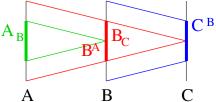
Figure 41: (Color online) The graphic representation of $A\to B$ and $A\to B\to C$.

Figure 42: (Color online) The graphic representation of $0\to A\to B\to C\to 0$, where $A_{B}=1$, $A\sim B^{A}=B_{C}$, and $C^{B}=C$.

We may also assume that $G$ has a non-trivial action on the modules $\mathbb{R}$ and $\mathbb{Z}$ (which are renamed $\mathbb{R}_{T}$ and $\mathbb{Z}_{T}$):

$$g\cdot n =s(g)n,\ \ \ n\in\mathbb{Z}_{T},$$

$$g\cdot x =s(g)x,\ \ \ x\in\mathbb{R}_{T},$$ (228)

where $s(g)=\pm 1$. We have

$$0\to\mathbb{Z}_{T}\to\mathbb{R}_{T}\to\mathbb{R}_{T}/\mathbb{Z}_{T}\to 0,$$ (229)

and

$$...\to \hat{\cal H}^{0}(G,\mathbb{Z}_{T})\to\hat{\cal H}^{0}(G,\mathbb{R}_{T})\to\hat{\cal H}^{0}(G,U_{T}(1))\to$$

$$\hat{\cal H}^{1}(G,\mathbb{Z}_{T})\to\hat{\cal H}^{1}(G,\mathbb{R}_{T})\to\hat{\cal H}^{1}(G,U_{T}(1))\to$$

$$\hat{\cal H}^{2}(G,\mathbb{Z}_{T})\to\hat{\cal H}^{2}(G,\mathbb{R}_{T})\to\hat{\cal H}^{2}(G,U_{T}(1))\to...$$ (230)

where we have used $\mathbb{R}_{T}/\mathbb{Z}_{T}=U_{T}(1)$. Since $\hat{\cal H}^{d}(G,\mathbb{R}_{T})=\mathbb{Z}_{1}$ when $G$ is a finite group or a compact Lie group, we have

$$0\to\hat{\cal H}^{d}(G,U_{T}(1))\to\hat{\cal H}^{d+1}(G,\mathbb{Z}_{T})\to 0$$ (231)

So $\hat{\cal H}^{d}(G,U_{T}(1))=\hat{\cal H}^{d+1}(G,\mathbb{Z}_{T})$ for any finite group or compact Lie group $G$. (On page 35 of LABEL:CS, it is stated that ${\cal H}^{d}(G,U(1))={\cal H}^{d+1}(G,\mathbb{Z})=H^{d+1}(BG,\mathbb{Z})$ for compact Lie group $G$.)

J.4.3 Module and $G$-module

In the next subsection, we are going to describe Künneth formula for group cohomology. As a preparation for the description, we will discuss the concepts of module and $G$-module here.

The concept of module is a generalization of the notion of vector space. Since two vectors can add, two elements in a module $M$, $a,b\in M$, also support an additive  +  operation:

$$a\,\text{\bf\tt+}\,b\in M.$$ (232)

The  +  operation commute and has inverse. So  +  is an Abelian group multiplication. The module $M$ equipped with the  +  operation is an Abelian group.

Vector spaces also have a scaler product operation, so do modules. The coefficients $n$ that we can multiply to elements $a$ in a module form a ring $R$. We will use  *  to describe the scaler product operation: $n\,\text{\bf\tt*}\,a\in M$, $n\in R$ and $a\in M$.

A ring $R$ is a set equipped with two binary operations: addition $+$ : $R\times R\to R$ and multiplication $\cdot$: $R\times R\to R$, where $\cdot$ may not have a inverse. A ring becomes a field if $\cdot$ does have an inverse, except for the additive identity “0”.

The scaler product  *  satisfies, for $n,m\in R$ and $a,b\in M$,

$$n\,\text{\bf\tt*}\,(a\,\text{\bf\tt+}\,b) =(n\,\text{\bf\tt*}\,a)\,\text{\bf\tt+}\,(n\,\text{\bf\tt*}\,b),$$

$$(n+m)\,\text{\bf\tt*}\,a =(n\,\text{\bf\tt*}\,a)\,\text{\bf\tt+}\,(m\,\text{\bf\tt*}\,a),$$

$$(n\cdot m)\,\text{\bf\tt*}\,a =n\,\text{\bf\tt*}\,(m\,\text{\bf\tt*}\,a),$$ (233)

$$1_{R}\,\text{\bf\tt*}\,a =a,\text{ if $R$ has multiplicative identity }1_{R}.$$

We will call the structure defined by $(M,R,\,\text{\bf\tt+}\,,\,\text{\bf\tt*}\,)$ a module $M$ over $R$.

A module over $R$ is $R$-free if the module has a basis (a linearly independent generating set): there exist elements $x_{1},x_{2},...\in M$, such that for every element $a\in M$, there is a unique set $n_{i}\in R$ such that $a=(n_{1}\,\text{\bf\tt*}\,x_{1})\,\text{\bf\tt+}\,(n_{2}\,\text{\bf\tt*}\,x_{2})\,\text{\bf\tt+}\,......$.

Here are some example of modules. A ring $R$ is a module over itself. Another simple example is $\mathbb{Z}$ over $\mathbb{Z}$. The module $\mathbb{Z}$ over $\mathbb{Z}$ is a free module. The basis set contains only one element $1$. The third example is the module $\mathbb{Z}_{2}$ over $\mathbb{Z}$. Such a module is not free, since if we choose $1$ as the basis, the element $0\in\mathbb{Z}_{2}$ can have several expressions: $0=0\times 1\text{ mod }2=2\times 1\text{ mod }2$. However, the module $\mathbb{Z}_{2}$ over $\mathbb{Z}_{2}$ is a free module with basis $1$.

The module that we are going to use in this paper is formed by pure complex phases $M=U(1)$. It is a module over $\mathbb{Z}$. The  +  and  *  operations are defined as

$$a\,\text{\bf\tt+}\,b=ab,\ \ \ \ n\,\text{\bf\tt*}\,a=a^{n},\ \ \ \ a,b\in U(1),\ n\in\mathbb{Z}.$$ (234)

Just like vector spaces, we can define direct sum of two modules, $M_{1}$ over $R$ and $M_{2}$ over $R$, which produces a third module $M_{3}$ over $R$. As a space, $M_{3}$ is given by $M_{3}=M_{1}\times M_{2}$. The  +  and  *  operations on $M_{3}=M_{1}\times M_{2}$ are given by

$$(a_{1},a_{2})\,\text{\bf\tt+}\,(b_{1},b_{2}) =(a_{1}\,\text{\bf\tt+}\,b_{1},a_{2}\,\text{\bf\tt+}\,b_{2}),$$

$$n\,\text{\bf\tt*}\,(a_{1},a_{2}) =(n\,\text{\bf\tt*}\,a_{1},n\,\text{\bf\tt*}\,a_{2}),$$

$$n\in R,\ \ a_{1},b_{1} \in M_{1},\ \ a_{2},b_{2}\in M_{2}.$$ (235)

The resulting module is denoted as $M_{1}\oplus M_{2}$. However, in this paper (see Table 1), we will use $M_{1}\times M_{2}$ to denote $M_{1}\oplus M_{2}$. Say, for module $\mathbb{Z}_{n}$ over $\mathbb{Z}$, $\mathbb{Z}_{n}\times Z_{m}=\mathbb{Z}_{n}\oplus\mathbb{Z}_{m}$ and $\mathbb{Z}_{n}^{2}=\mathbb{Z}_{n}\times Z_{n}=\mathbb{Z}_{n}\oplus\mathbb{Z}_{n}$, etc .

We can also define tensor product $\otimes_{R}$, which maps two modules, $M_{1}$ over $R$ and $M_{2}$ over $R$, to a third module $M_{3}$ over $R$: $M_{3}=M_{1}\otimes_{R}M_{2}$. If the two modules $M_{1}$ and $M_{2}$ are free with basis $\{x_{i}\}$ and $\{y_{i}\}$ respectively, then their tensor product $M_{3}=M_{1}\otimes_{R}M_{2}$ is simply a module over $R$ with $\{x_{i}\otimes y_{j}\}$ as basis. If the modules $M_{1}$ and/or $M_{2}$ are not free, then their tensor product is more complicated: $M_{3}=M_{1}\otimes_{R}M_{2}$ is module over $R$ whose elements have the form

$$[n_{1}\,\text{\bf\tt*}\,(a_{1}\otimes_{R}b_{1})]\,\text{\bf\tt+}\,[n_{2}\,\text{\bf\tt*}\,(a_{2}\otimes_{R}b_{2})]\,\text{\bf\tt+}\,......$$

$$n_{i}\in R,\ \ \ \ a_{i}\in M_{1},\ \ \ b_{i}\in M_{2},$$ (236)

subject to the following reduction relation

$$((a_{1}\,\text{\bf\tt+}\,a_{2})\otimes_{R}b)\ \,\text{\bf\tt-}\,(a_{1}\otimes_{R}b)\ \,\text{\bf\tt-}\,(a_{2}\otimes_{R}b)=0,$$

$$(a\otimes_{R}(b_{1}\,\text{\bf\tt+}\,b_{2}))\ \,\text{\bf\tt-}\,(a\otimes_{R}b_{1})\ \,\text{\bf\tt-}\,(a\otimes_{R}b_{2}))=0,$$

$$n\,\text{\bf\tt*}\,(a\otimes_{R}b)=((n\,\text{\bf\tt*}\,a)\otimes_{R}b)=(a\otimes_{R}(n\,\text{\bf\tt*}\,b)).$$ (237)

Such a definition allows us to obtain the following result:

$$\mathbb{Z}\otimes_{\mathbb{Z}}M=M\otimes_{\mathbb{Z}}\mathbb{Z}=M,$$

$$\mathbb{Z}_{n}\otimes_{\mathbb{Z}}M=M\otimes_{\mathbb{Z}}\mathbb{Z}_{n}=M/nM,$$

$$\mathbb{Z}_{m}\otimes_{\mathbb{Z}}\mathbb{Z}_{n}=\mathbb{Z}_{(m,n)},$$

$$(A\times B)\otimes_{R}M=(A\otimes_{R}M)\times(B\otimes_{R}M),$$

$$M\otimes_{R}(A\times B)=(M\otimes_{R}A)\times(M\otimes_{R}B);$$ (238)

where $(m,n)$ is the greatest common divisor of $m$ and $n$. In the above $\times$ really represents $\oplus$.

We can also define torsion product $\text{Tor}_{1}^{R}(,)$, which maps two modules, $M_{1}$ over $R$ and $M_{2}$ over $R$, to a third module $M_{3}$ over $R$: $M_{3}=\text{Tor}_{1}^{R}(M_{1},M_{2})$. We will not discuss the definition of the torsion product. We just list some simple results here:

$$\text{Tor}_{1}^{R}(A,B)\simeq\text{Tor}_{1}^{R}(B,A),$$

$$\text{Tor}_{1}^{\mathbb{Z}}(\mathbb{Z},M)=\text{Tor}_{1}^{\mathbb{Z}}(M,\mathbb{Z})=0,$$

$$\text{Tor}_{1}^{\mathbb{Z}}(\mathbb{Z}_{n},M)=\{m\in M|nm=0\},$$

$$\text{Tor}_{1}^{\mathbb{Z}}(\mathbb{Z}_{m},\mathbb{Z}_{n})=\mathbb{Z}_{(m,n)},$$

$$\text{Tor}_{1}^{R}(A\times B,M)=\text{Tor}_{1}^{R}(A,M)\times\text{Tor}_{1}^{R}(B,M),$$

$$\text{Tor}_{1}^{R}(M,A\times B)=\text{Tor}_{1}^{R}(M,A)\times\text{Tor}_{1}^{R}(M,B),$$ (239)

Again $\times$ really represents $\oplus$.

A $G$-module over $R$ is a module over $R$ that also admits a group $G$ action: $g\cdot a\in M$ for $a\in M$ and $g\in G$. The group action is compatible with the  +  and  *  operations:

$$g\cdot(a\,\text{\bf\tt+}\,b)=(g\cdot a)\,\text{\bf\tt+}\,(g\cdot b),\ \ \ \ g\cdot(n\,\text{\bf\tt*}\,a)=n\,\text{\bf\tt*}\,(g\cdot a).$$ (240)

In the group cohomology ${\cal H}^{d}(G,M)$, $M$ is a $G$-module over $R$. In fact, ${\cal H}^{d}(G,M)$ is also a $G$-module over $R$.

J.4.4 Künneth formula for group cohomology

Now, we are ready to describe the Künneth formula for group cohomology. Let $M$ (resp. $M^{\prime}$) be an arbitrary $G$-module (resp. $G^{\prime}$-module) over a principal ideal domain $R$. We also assume that either $M$ or $M^{\prime}$ is $R$-free. Then we have a Künneth formula for group cohomologyG0691 ; Kunn

$$0 \rightarrow\prod_{p=0}^{d}{\cal H}^{p}(G,M)\otimes_{R}{\cal H}^{d-p}(G^{\prime},M^{\prime})$$

$$\rightarrow{\cal H}^{d}(G\times G^{\prime},M\otimes_{R}M^{\prime})$$

$$\rightarrow\prod_{p=0}^{d+1}\text{Tor}_{1}^{R}({\cal H}^{p}(G,M),{\cal H}^{d-p+1}(G^{\prime},M^{\prime}))\rightarrow 0$$ (241)

If both $M$ and $M^{\prime}$ are $R$-free, then the sequence splits and we have

$$\ \ \ \ {\cal H}^{d}(G\times G^{\prime},M\otimes_{R}M^{\prime})$$

$$=\Big{[}\prod_{p=0}^{d}{\cal H}^{p}(G,M)\otimes_{R}{\cal H}^{d-p}(G^{\prime},M^{\prime})\Big{]}\times$$

$$\ \ \ \ \ \ \Big{[}\prod_{p=0}^{d+1}\text{Tor}_{1}^{R}({\cal H}^{p}(G,M),{\cal H}^{d-p+1}(G^{\prime},M^{\prime}))\Big{]}.$$ (242)

If $R$ is a field $K$, we have

$$\ \ \ \ {\cal H}^{d}(G\times G^{\prime},M\otimes_{K}M^{\prime})$$

$$=\Big{[}\prod_{p=0}^{d}{\cal H}^{p}(G,M)\otimes_{K}{\cal H}^{d-p}(G^{\prime},M^{\prime})\Big{]}.$$ (243)

For the cases studied in this paper, we have $R=M=\mathbb{Z}$ (ie $G$ acts trivially on $\mathbb{Z}$) and $M^{\prime}=\mathbb{Z}_{T}$ (ie $G^{\prime}$ may act non-trivially on $\mathbb{Z}_{T}$). So $M\otimes_{\mathbb{Z}}M^{\prime}=\mathbb{Z}_{T}$, on which $G$ acts trivially and $G^{\prime}$ may act non-trivially. Also the sequence splits.

J.4.5 Cup product for group cohomology

Consider two cochains $\nu_{n_{1}}\in{\cal C}^{n_{1}}(G,M_{1})$ and $\nu_{n_{2}}\in{\cal C}^{n_{2}}(G,M_{2})$. From $\nu_{n_{1}}$ and $\nu_{n_{2}}$, we can construct a third cochain $\nu_{n_{1}+n_{2}}\in{\cal C}^{n_{1}+n_{2}}(G,M_{1}\otimes_{\mathbb{Z}}M_{2})$:

$$\ \ \ \ \nu_{n_{1}+n_{2}}(g_{0},g_{1},...,g_{n_{1}+n_{2}})$$ (244)

$$=\nu_{n_{1}}(g_{0},g_{1},...,g_{n_{1}})\otimes_{\mathbb{Z}}\nu_{n_{2}}(g_{n_{1}},g_{n_{1}+1},...,g_{n_{1}+n_{2}}).$$

The above mapping ${\cal C}^{n_{1}}(G,M_{1})\times{\cal C}^{n_{2}}(G,M_{2})\to{\cal C}^{n_{1}+n_{2}}(G,M_{1}\otimes_{\mathbb{Z}}M_{2})$ is called the cup product and is denoted as

$$\nu_{n_{1}+n_{2}}=\nu_{n_{1}}\cup\nu_{n_{2}}.$$ (245)

The cup product has the following nice property

$$d\nu_{n_{1}+n_{2}}=[(d\nu_{n_{1}})\cup\nu_{n_{2}}]\,\text{\bf\tt+}\,[(-)^{n_{1}}\,\text{\bf\tt*}\,\nu_{n_{1}}\cup(d\nu_{n_{2}})],$$ (246)

where

$$\ \ \ \ (d\nu_{n})(g_{0},...,g_{n+1})$$

$$=\,\text{\bf\tt+}\,_{i=0}^{n+1}[(-)^{i}\,\text{\bf\tt*}\,\nu_{n}(g_{0},...,\hat{g}_{i},...,g_{n+1})].$$ (247)

where the sequence $g_{0},...,\hat{g}_{i},...,g_{n+1}$ is the sequence $g_{0},...,g_{n+1}$ with $g_{i}$ removed. So if $\nu_{n_{1}}$ and $\nu_{n_{2}}$ are cocycles $\nu_{n_{1}}\cup\nu_{n_{2}}$ is also a cocycle. Thus the cup product defines the mapping

$${\cal H}^{n_{1}}(G,M_{1})\times{\cal H}^{n_{2}}(G,M_{2})\to{\cal H}^{n_{1}+n_{2}}(G,M_{1}\otimes_{\mathbb{Z}}M_{2}).$$ (248)

As a map between classes of cocycles, the cup product satisfiesRS

$$\nu_{n_{1}}\cup\nu_{n_{2}}=(-)^{n_{1}n_{2}}\,\text{\bf\tt*}\,(\nu_{n_{2}}\cup\nu_{n_{1}}),$$

$$(\nu_{n_{1}}\cup\nu_{n_{2}})\cup\nu_{n_{3}}=\nu_{n_{1}}\cup(\nu_{n_{2}}\cup\nu_{n_{3}}).$$ (249)

Let

$$H^{*}(G,M)=H^{0}(G,M)\oplus H^{1}(G,M)\oplus...$$ (250)

$H^{*}(G,M)$ has an additive operation  +  inherited from the module $M$. The cup product provided an multiplicative operation on $H^{*}(G,M)$. So $H^{*}(G,M)$ with the additive operation  +  and the multiplicative operation $\cup$ is a ring which is called the group cohomology ring for the group $G$.

J.5 Group cohomology of $Z_{m}\times Z_{n}$

Let us first calculate ${\cal H}^{d}[Z_{m}\times Z_{n},\mathbb{Z}]$. Using eqn. (J.4.4), we find that

$${\cal H}^{d}(\mathbb{Z}_{m}\times Z_{n};\mathbb{Z})\cong\left(\prod_{i=0}^{d}{\cal H}^{i}(Z_{m};\mathbb{Z})\otimes_{\mathbb{Z}}{\cal H}^{d-i}(Z_{n};\mathbb{Z})\right)$$

$$\times\left(\prod_{p=0}^{n+1}\text{Tor}_{1}^{\mathbb{Z}}({\cal H}^{p}(Z_{m};\mathbb{Z}),{\cal H}^{d+1-p}(Z_{n};\mathbb{Z}))\right).$$ (251)

The above can be calculated using eqn. (208) and the simple properties of the tensor product $\otimes_{\mathbb{Z}}$ and torsion product $\text{Tor}_{1}^{\mathbb{Z}}$ in eqn. (J.4.3) and eqn. (J.4.3). For example

$$\ \ \ \ {\cal H}^{0}(\mathbb{Z}_{m}\times Z_{n};\mathbb{Z})$$

$$\cong\left(\mathbb{Z}\otimes_{\mathbb{Z}}\mathbb{Z}\right)\times\text{Tor}_{1}^{\mathbb{Z}}(\mathbb{Z}_{1},\mathbb{Z})\times\text{Tor}_{1}^{\mathbb{Z}}(\mathbb{Z},\mathbb{Z}_{1})$$

$$=\mathbb{Z}.$$ (252)

$$\ \ \ \ {\cal H}^{1}(\mathbb{Z}_{m}\times Z_{n};\mathbb{Z})$$

$$\cong\left(\mathbb{Z}_{1}\otimes_{\mathbb{Z}}\mathbb{Z}\right)\times\left(\mathbb{Z}\otimes_{\mathbb{Z}}\mathbb{Z}_{1}\right)\times\text{Tor}_{1}^{\mathbb{Z}}(\mathbb{Z},\mathbb{Z}_{n})$$

$$\ \ \ \ \ \ \ \ \times\text{Tor}_{1}^{\mathbb{Z}}(\mathbb{Z}_{1},\mathbb{Z}_{1})\times\text{Tor}_{1}^{\mathbb{Z}}(\mathbb{Z}_{m},\mathbb{Z})$$

$$=\mathbb{Z}_{1}.$$ (253)

$$\ \ \ \ {\cal H}^{2}(\mathbb{Z}_{m}\times Z_{n};\mathbb{Z})$$

$$\cong\left(\mathbb{Z}_{m}\otimes_{\mathbb{Z}}\mathbb{Z}\right)\times\left(\mathbb{Z}\otimes_{\mathbb{Z}}\mathbb{Z}_{n}\right)\times\text{Tor}_{1}^{\mathbb{Z}}(\mathbb{Z},\mathbb{Z}_{1})\times\text{Tor}_{1}^{\mathbb{Z}}(\mathbb{Z}_{1},\mathbb{Z}_{n})$$

$$\ \ \ \ \ \ \ \ \times\text{Tor}_{1}^{\mathbb{Z}}(\mathbb{Z}_{m},\mathbb{Z}_{1})\times\text{Tor}_{1}^{\mathbb{Z}}(\mathbb{Z}_{1},\mathbb{Z})$$

$$=\mathbb{Z}_{m}\times\mathbb{Z}_{n}.$$ (254)

Using the relation ${\cal H}^{d}(\mathbb{Z}_{m}\times Z_{n};U(1))={\cal H}^{d+1}(\mathbb{Z}_{m}\times Z_{n};\mathbb{Z})$, $d>0$, we find

$${\cal H}^{d}[Z_{m}\times Z_{n},U(1)]=\begin{cases}U(1)&d=0,\\ \mathbb{Z}^{d/2}_{(m,n)}&d=\text{ even}\\ \mathbb{Z}_{m}\times\mathbb{Z}_{n}\times\mathbb{Z}^{(d-1)/2}_{(m,n)}&d=\text{ odd}.\end{cases}$$ (255)

This agrees with eqn. (215).

J.6 Group cohomology of $Z_{2}^{T}\times Z_{n}$

Let us first calculate ${\cal H}^{d}[Z_{2}^{T}\times Z_{n},\mathbb{Z}_{T}]$ where $Z_{2}^{T}$ acts on $\mathbb{Z}_{T}$ non-trivially (see eqn. (213)). Using eqn. (J.4.4), we find that

$${\cal H}^{d}(\mathbb{Z}_{2}^{T}\times Z_{n};\mathbb{Z}_{T})\cong\left(\prod_{i=0}^{d}{\cal H}^{i}(Z_{2}^{T};\mathbb{Z}_{T})\otimes_{\mathbb{Z}}{\cal H}^{d-i}(Z_{n};\mathbb{Z})\right)$$

$$\times\left(\prod_{p=0}^{n+1}\text{Tor}_{1}^{\mathbb{Z}}({\cal H}^{p}(Z_{2}^{T};\mathbb{Z}_{T}),{\cal H}^{d+1-p}(Z_{n};\mathbb{Z}))\right).$$ (256)

Using the relation ${\cal H}^{d}(\mathbb{Z}_{2}^{T}\times Z_{n};U_{T}(1))={\cal H}^{d+1}(\mathbb{Z}_{2}^{T}\times Z_{n};\mathbb{Z}_{T})$, $d>0$, we find

$${\cal H}^{d}[Z_{2}^{T}\times Z_{n},U_{T}(1)]=\begin{cases}\mathbb{Z}_{2}\times\mathbb{Z}^{d/2}_{(2,n)}&d=\text{ even}\\ \mathbb{Z}^{(d+1)/2}_{(2,n)}&d=\text{ odd}.\end{cases}$$ (257)

When $n$ is odd, this agrees with eqn. (217).

J.7 Group cohomology of $D_{2h}$

The group $D_{2h}$ is the same as $Z_{2}\times Z_{2}\times Z_{2}^{T}$. So we can use the Künneth formula and the results in subsection J.5 to calculate ${\cal H}^{d}[D_{2h},U_{T}(1)]$. Let us first calculate ${\cal H}^{d}[Z_{m}\times Z_{n}\times Z_{2}^{T},\mathbb{Z}_{T}]$:

$$\ \ \ \ {\cal H}^{0}[Z_{m}\times Z_{n}\times Z_{2}^{T},\mathbb{Z}_{T}]\cong\mathbb{Z}_{1}.$$ (258)

$$\ \ \ \ {\cal H}^{1}[Z_{m}\times Z_{n}\times Z_{2}^{T},\mathbb{Z}_{T}]\cong(\mathbb{Z}\otimes_{\mathbb{Z}}\mathbb{Z}_{2})=\mathbb{Z}_{2}.$$ (259)

$$\ \ \ \ {\cal H}^{2}[Z_{m}\times Z_{n}\times Z_{2}^{T},\mathbb{Z}_{T}]$$

$$\cong\text{Tor}_{1}^{\mathbb{Z}}(\mathbb{Z}_{m}\times\mathbb{Z}_{n},\mathbb{Z}_{2})$$

$$=\text{Tor}_{1}^{\mathbb{Z}}(\mathbb{Z}_{m},\mathbb{Z}_{2})\times\text{Tor}_{1}^{\mathbb{Z}}(\mathbb{Z}_{n},\mathbb{Z}_{2})$$

$$=\mathbb{Z}_{(2,m)}\times\mathbb{Z}_{(2,n)}.$$ (260)

$$\ \ \ \ {\cal H}^{3}[Z_{m}\times Z_{n}\times Z_{2}^{T},\mathbb{Z}_{T}]$$

$$\cong(\mathbb{Z}\otimes_{\mathbb{Z}}\mathbb{Z}_{2})\times[(\mathbb{Z}_{m}\times\mathbb{Z}_{n})\otimes_{\mathbb{Z}}\mathbb{Z}_{2}]\times\text{Tor}_{1}^{\mathbb{Z}}(\mathbb{Z}_{(m,n)},\mathbb{Z}_{2})$$

$$=\mathbb{Z}_{2}\times\mathbb{Z}_{(2,m)}\times\mathbb{Z}_{(2,n)}\times\mathbb{Z}_{(m,n)}.$$ (261)

$$\ \ \ \ {\cal H}^{4}[Z_{m}\times Z_{n}\times Z_{2}^{T},\mathbb{Z}_{T}]$$

$$\cong(\mathbb{Z}_{(m,n)}\otimes_{\mathbb{Z}}\mathbb{Z}_{2})\times\text{Tor}_{1}^{\mathbb{Z}}(\mathbb{Z}_{m}\times\mathbb{Z}_{n},\mathbb{Z}_{2})$$

$$\ \ \ \ \ \ \ \ \ \times\text{Tor}_{1}^{\mathbb{Z}}(\mathbb{Z}_{m}\times\mathbb{Z}_{n}\times\mathbb{Z}_{(m,n)},\mathbb{Z}_{2})$$

$$=\mathbb{Z}^{2}_{(2,m,n)}\times\mathbb{Z}^{2}_{(2,m)}\times\mathbb{Z}^{2}_{(2,n)}.$$ (262)

$$\ \ \ \ {\cal H}^{5}[Z_{m}\times Z_{n}\times Z_{2}^{T},\mathbb{Z}_{T}]$$

$$\cong(\mathbb{Z}\otimes_{\mathbb{Z}}\mathbb{Z}_{2})\times[(\mathbb{Z}_{m}\times\mathbb{Z}_{n})\otimes_{\mathbb{Z}}\mathbb{Z}_{2}]$$

$$\ \ \ \ \ \ \ \ \ \times[(\mathbb{Z}_{m}\times\mathbb{Z}_{n}\times\mathbb{Z}_{(m,n)})\otimes_{\mathbb{Z}}\mathbb{Z}_{2}]$$

$$\ \ \ \ \ \ \ \ \ \times\text{Tor}_{1}^{\mathbb{Z}}(\mathbb{Z}_{(m,n)},\mathbb{Z}_{2})\times\text{Tor}_{1}^{\mathbb{Z}}(\mathbb{Z}^{2}_{(m,n)},\mathbb{Z}_{2})$$

$$=\mathbb{Z}_{2}\times\mathbb{Z}^{4}_{(2,m,n)}\times\mathbb{Z}^{2}_{(2,m)}\times\mathbb{Z}^{2}_{(2,n)}.$$ (263)

This gives us

$$\ \ \ \ {\cal H}^{1}[Z_{m}\times Z_{n}\times Z_{2}^{T},U_{T}(1)]$$

$$\cong\mathbb{Z}_{(2,m)}\times\mathbb{Z}_{(2,n)}.$$ (264)

$$\ \ \ \ {\cal H}^{2}[Z_{m}\times Z_{n}\times Z_{2}^{T},U_{T}(1)]$$

$$\cong\mathbb{Z}_{2}\times\mathbb{Z}_{(2,m)}\times\mathbb{Z}_{(2,n)}\times\mathbb{Z}_{(m,n)}.$$ (265)

$$\ \ \ \ {\cal H}^{3}[Z_{m}\times Z_{n}\times Z_{2}^{T},U_{T}(1)]$$

$$\cong\mathbb{Z}^{2}_{(2,m,n)}\times\mathbb{Z}^{2}_{(2,m)}\times\mathbb{Z}^{2}_{(2,n)}.$$ (266)

$$\ \ \ \ {\cal H}^{4}[Z_{m}\times Z_{n}\times Z_{2}^{T},U_{T}(1)]$$

$$\cong\mathbb{Z}_{2}\times\mathbb{Z}^{4}_{(2,m,n)}\times\mathbb{Z}^{2}_{(2,m)}\times\mathbb{Z}^{2}_{(2,n)}.$$ (267)

The results ${\cal H}^{1}[Z_{2}\times Z_{2}\times Z_{2}^{T},U_{T}(1)]={\cal H}^{1}[D_{2h},U_{T}(1)]=\mathbb{Z}_{2}^{2}$ and ${\cal H}^{2}[Z_{2}\times Z_{2}\times Z_{2}^{T},U_{T}(1)]={\cal H}^{2}[D_{2h},U_{T}(1)]=\mathbb{Z}_{2}^{4}$ agrees with those in LABEL:CGW1123,LCW1121 obtained through direct calculations.

J.8 Group cohomology of $U(1)$

To calculate ${\cal H}^{d}[U(1),U(1)]$ (the Borel cohomology) directly from the algebraic definition is very tricky since $U(1)$ has infinite uncountable many elements. Here, we will use a physical argument to calculate it by first calculating ${\cal H}^{d}[Z_{n},U(1)]$, and then let $n\to\infty$. This way, we find

$${\cal H}^{d}[U(1),U(1)]=\begin{cases}U(1)&\text{ if }d=0,\\ \mathbb{Z}_{1}&\text{ if }d=0\text{ mod }2,\ \ d>0\\ \mathbb{Z}&\text{ if }d=1\text{ mod }2.\end{cases}$$ (268)

In LABEL:PM, it is stated that

$${\cal H}^{d}[U(1),\mathbb{Z}]=\begin{cases}\mathbb{Z}&\text{ if }d=0\text{ mod }2,\\ \mathbb{Z}_{1}&\text{ if }d=1\text{ mod }2.\end{cases}$$ (269)

This is consistent with eqn. (268) since ${\cal H}^{d}[U(1),U(1)]={\cal H}^{d+1}[U(1),\mathbb{Z}]$.

We note that the 1D representations of $U(1)$, $M(U_{\theta})=\hskip 1.0pt\mathrm{e}^{n\hskip 1.0pt\mathrm{i}\hskip 1.0pt\theta}$, where the $U(1)$ group elements are denoted as $U_{\theta}$, are labeled by $n\in\mathbb{Z}$. Also, $U(1)$ has no non-trivial projective representation. This is consistent with the above results: ${\cal H}^{1}[U(1),U_{T}(1)]=\mathbb{Z}$ and ${\cal H}^{2}[U(1),U_{T}(1)]=\mathbb{Z}_{1}$.

J.9 Group cohomology of $Z_{2}^{T}\times U(1)$

As pointed out in the section C, a spin system with time reversal and $U(1)$ (say generated by $S_{z}$) symmetries has a symmetry group $U(1)\times Z_{2}^{T}$. To find the SPT phases of such a bosonic system, we need to calculate ${\cal H}^{d}[U(1)\times Z_{2}^{T},U_{T}(1)]$. We simply need to repeat the calculation of ${\cal H}^{d}[Z_{2}^{T}\times Z_{n},\mathbb{Z}_{T}]$ by replacing $\mathbb{Z}_{n}$ with $\mathbb{Z}$. We note that $\mathbb{Z}_{2}\otimes_{\mathbb{Z}}\mathbb{Z}_{n}=\mathbb{Z}_{(2,n)}$ and $\text{Tor}_{1}^{\mathbb{Z}}(\mathbb{Z}_{2},\mathbb{Z}_{n})=\mathbb{Z}_{(2,n)}$, while $\mathbb{Z}_{2}\otimes_{\mathbb{Z}}\mathbb{Z}=\mathbb{Z}_{2}$ and $\text{Tor}_{1}^{\mathbb{Z}}(\mathbb{Z}_{2},\mathbb{Z})=\mathbb{Z}_{1}$. So we find

$${\cal H}^{d}[Z_{2}^{T}\times U(1),\mathbb{Z}_{T}]=\begin{cases}\mathbb{Z}_{1}&d=0,\\ \mathbb{Z}_{1}&d=\text{ even}\\ \mathbb{Z}^{\frac{d+1}{2}}_{2}&d=\text{ odd}.\end{cases}$$ (270)

Since ${\cal H}^{d}[Z_{2}^{T}\times U(1),\mathbb{R}_{T}]=\mathbb{Z}_{1}$, we have ${\cal H}^{d}[Z_{2}^{T}\times U(1),U_{T}(1)]={\cal H}^{d+1}[Z_{2}^{T}\times U(1),\mathbb{Z}_{T}]$, and

$${\cal H}^{d}[Z_{2}^{T}\times U(1),U_{T}(1)]=\begin{cases}\mathbb{Z}^{\frac{d+2}{2}}_{2}&d=\text{ even},\\ \mathbb{Z}_{1}&d=\text{ odd}.\end{cases}$$ (271)

This can be obtained from eqn. (257) by taking $n\to\infty$ and choosing $\lim_{n\to\infty}\mathbb{Z}_{(2,n)}=\mathbb{Z}_{2}$ for $d=$ even, and $\lim_{n\to\infty}\mathbb{Z}_{(2,n)}=\mathbb{Z}_{1}$ for $d=$ odd.

J.10 Group cohomology of $U(1)\rtimes Z_{2}^{T}$

As pointed out in the section C, a bosonic system with time reversal symmetry and boson number conservation has a symmetry group $U(1)\rtimes Z_{2}^{T}$. To find the SPT phases of such a bosonic system, we need to calculate ${\cal H}^{d}[U(1)\rtimes Z_{2}^{T},U_{T}(1)]$. In the last subsection, we calculated ${\cal H}^{d}[U(1)\times Z_{2}^{T},U_{T}(1)]$. In those two cases, $Z_{2}^{T}$ has a non-trivial action on the module $M=U_{T}(1)$.

The other two related cohomology groups are ${\cal H}^{d}[U(1)\times Z_{2},U(1)]$ and ${\cal H}^{d}[U(1)\rtimes Z_{2},U(1)]$, where the $Z_{2}$ is a usual unitary symmetry. In those two cases, $Z_{2}$ has a trivial action on the module $M=U(1)$.

In this section, we will use spectral sequence method to calculate the above four cohomology groups from the following facts:

$${\cal H}^{2p}[U(1),\mathbb{Z}] =\mathbb{Z}, {\cal H}^{2p+1}[U(1),\mathbb{Z}] =0,$$

$${\cal H}^{2p}[\mathbb{Z}_{n},\mathbb{Z}] =\mathbb{Z}_{n}, {\cal H}^{2p+1}[\mathbb{Z}_{2},\mathbb{Z}] =0,$$

$${\cal H}^{2p}[\mathbb{Z}_{2}^{T},\mathbb{Z}_{T}] =0, {\cal H}^{2p+1}[\mathbb{Z}_{2}^{T},\mathbb{Z}_{T}] =\mathbb{Z}_{2}.$$ (272)

Let $G$ be one of the $U(1)\times Z_{2}$, $U(1)\rtimes Z_{2}$, $U(1)\times Z_{2}^{T}$, and $U(1)\rtimes Z_{2}^{T}$. From the exact sequence of the groups $1\to U(1)\to G\to Z_{2}\to 1$, we have the following $E^{p,q}_{2}={\cal H}^{p}[Z_{2},{\cal H}^{q}[U(1),M]]$ page:

$$\begin{matrix}{\cal H}^{0}[Z_{2},{\cal H}^{3}[U(1),M]]&{\cal H}^{1}[Z_{2},{\cal H}^{3}[U(1),M]]&{\cal H}^{2}[Z_{2},{\cal H}^{3}[U(1),M]]&{\cal H}^{3}[Z_{2},{\cal H}^{3}[U(1),M]]\\ {\cal H}^{0}[Z_{2},{\cal H}^{2}[U(1),M]]&{\cal H}^{1}[Z_{2},{\cal H}^{2}[U(1),M]]&{\cal H}^{2}[Z_{2},{\cal H}^{2}[U(1),M]]&{\cal H}^{3}[Z_{2},{\cal H}^{2}[U(1),M]]\\ {\cal H}^{0}[Z_{2},{\cal H}^{1}[U(1),M]]&{\cal H}^{1}[Z_{2},{\cal H}^{1}[U(1),M]]&{\cal H}^{2}[Z_{2},{\cal H}^{1}[U(1),M]]&{\cal H}^{3}[Z_{2},{\cal H}^{1}[U(1),M]]\\ {\cal H}^{0}[Z_{2},{\cal H}^{0}[U(1),M]]&{\cal H}^{1}[Z_{2},{\cal H}^{0}[U(1),M]]&{\cal H}^{2}[Z_{2},{\cal H}^{0}[U(1),M]]&{\cal H}^{3}[Z_{2},{\cal H}^{0}[U(1),M]]\\ \end{matrix}$$ (273)

To calculate ${\cal H}^{p}[Z_{2},{\cal H}^{q}[U(1),M]]$, we need to know how $Z_{2}$ acts on ${\cal H}^{q}[U(1),M]$ through how $Z_{2}$ acts on $U(1)$ group and $M$ module.

First we consider $U(1)\times Z_{2}$ group and module $M=\mathbb{Z}$. In this case, $Z_{2}$ acts on $U(1)$ group trivially and it acts on $M$ trivially. As a result, $Z_{2}$ acts on ${\cal H}^{q}[U(1),\mathbb{Z}]$ trivially: $T\cdot\alpha\to\alpha$, $\alpha\in{\cal H}^{q}[U(1),\mathbb{Z}_{T}]$. Note that ${\cal H}^{d}[U(1),\mathbb{Z}]=\mathbb{Z}$, ${\cal H}^{d}[\mathbb{Z}_{2},\mathbb{Z}]=\mathbb{Z}_{2}$ for $d=$ even and ${\cal H}^{d}[U(1),\mathbb{Z}_{T}]=\mathbb{Z}_{1}=0$, ${\cal H}^{d}[\mathbb{Z}_{2},\mathbb{Z}]=\mathbb{Z}_{1}=0$ for $d=$ odd. We obtain the following $E^{p,q}_{2}={\cal H}^{p}[Z_{2},{\cal H}^{q}[U(1),\mathbb{Z}]]$ page in the spectral sequence:

$$\begin{matrix}0&0&0&0&0&0&0&0\\ \mathbb{Z}&0&\mathbb{Z}_{2}&0&\mathbb{Z}_{2}&0&\mathbb{Z}_{2}&0\\ 0&0&0&0&0&0&0&0\\ \mathbb{Z}&0&\mathbb{Z}_{2}&0&\mathbb{Z}_{2}&0&\mathbb{Z}_{2}&0\\ 0&0&0&0&0&0&0&0\\ \mathbb{Z}&0&\mathbb{Z}_{2}&0&\mathbb{Z}_{2}&0&\mathbb{Z}_{2}&0\\ 0&0&0&0&0&0&0&0\\ \mathbb{Z}&0&\mathbb{Z}_{2}&0&\mathbb{Z}_{2}&0&\mathbb{Z}_{2}&0\\ \end{matrix}$$ (274)

In the $E_{2}^{p,q}$ page, we have spectral sequence

$$...\rightarrow E_{2}^{p,q}\rightarrow E_{2}^{p+2,q-1}\rightarrow...$$ (275)

generated by $d_{2}^{p,q}:E_{2}^{p,q}\to E_{2}^{p+2,q-1}$ such that $d_{2}^{p+2,q-1}d_{2}^{p,q}=0$. So the cohomology of $d_{2}^{p,q}$ produces the $E_{3}^{p,q}$ page: $E_{3}^{p,q}=\text{ker}d_{2}^{p,q}/\text{im}d_{2}^{p-2,q+1}$. We note that all the non trivial terms in the $E_{2}^{p,q}$ page are connected to an incoming zero and an outing zero. Thus $d_{2}^{p,q}=0$, which leads to $\text{ker}d_{2}^{p,q}=E_{2}^{p,q}$ and $\text{im}d_{2}^{p,q}=0$. So $E_{3}^{p,q}=E_{2}^{p,q}$. In the $E_{3}^{p,q}$ page, we have a spectral sequence

$$...\rightarrow E_{3}^{p,q}\rightarrow E_{3}^{p+3,q-2}\rightarrow...$$ (276)

and again all the non trivial terms in the $E_{3}^{p,q}$ page are connected to an incoming zero and an outing zero and $d_{3}^{p,q}=0$. So $E_{4}^{p,q}=E_{3}^{p,q}(=E_{2}^{p,q})$. This way, we can show that the $E_{2}^{p,q}$ page stabilizes: $E_{\infty}^{p,q}=E_{2}^{p,q}$. Using $E_{\infty}^{p,q}$ with $p+q=n$, we can calculate ${\cal H}^{n}[U(1)\times Z_{2},\mathbb{Z}]$, since ${\cal H}^{n}[U(1)\times Z_{2},\mathbb{Z}]$ has a filtration

$$0=H^{n}_{n+1}\subseteq H^{n}_{n}...\subseteq H^{n}_{1}\subseteq H^{n}_{0}={\cal H}^{n}[U(1)\times Z_{2},\mathbb{Z}],$$ (277)

such that $H^{n}_{p}/H^{n}_{p+1}=E_{\infty}^{p,n-p}$. Thus we have

$${\cal H}^{d}[U(1)\times Z_{2},\mathbb{Z}]=\begin{cases}\mathbb{Z}\times\mathbb{Z}^{d/2}_{2},&d=0\text{ mod }2,\\ \mathbb{Z}_{1},&d=1\text{ mod }2,\end{cases}$$ (278)

which gives

$${\cal H}^{d}[U(1)\times Z_{2},U(1)]=\begin{cases}U(1),&d=0,\\ \mathbb{Z}_{1},&d=0\text{ mod }2,\\ \mathbb{Z}\times\mathbb{Z}^{\frac{d+1}{2}}_{2},&d=1\text{ mod }2.\end{cases}$$ (279)

Next we consider $U(1)\times Z_{2}^{T}$ group and module $M=\mathbb{Z}_{T}$. In this case, $Z_{2}^{T}$ acts on $U(1)$ group trivially and it acts on $M$ non-trivially: $T\cdot n\to-n$, $n\in\mathbb{Z}_{T}$. As a result, $Z_{2}$ acts on ${\cal H}^{q}[U(1),\mathbb{Z}_{T}]$ non-trivially: $T\cdot\alpha\to-\alpha$, $\alpha\in{\cal H}^{q}[U(1),\mathbb{Z}_{T}]$. We obtain the following $E^{p,q}_{2}={\cal H}^{p}[Z_{2},{\cal H}^{q}[U(1),\mathbb{Z}_{T}]]$ page in the spectral sequence:

$$\begin{matrix}0&0&0&0&0&0&0&0\\ 0&\mathbb{Z}_{2}&0&\mathbb{Z}_{2}&0&\mathbb{Z}_{2}&0&\mathbb{Z}_{2}\\ 0&0&0&0&0&0&0&0\\ 0&\mathbb{Z}_{2}&0&\mathbb{Z}_{2}&0&\mathbb{Z}_{2}&0&\mathbb{Z}_{2}\\ 0&0&0&0&0&0&0&0\\ 0&\mathbb{Z}_{2}&0&\mathbb{Z}_{2}&0&\mathbb{Z}_{2}&0&\mathbb{Z}_{2}\\ 0&0&0&0&0&0&0&0\\ 0&\mathbb{Z}_{2}&0&\mathbb{Z}_{2}&0&\mathbb{Z}_{2}&0&\mathbb{Z}_{2}\\ \end{matrix}$$ (280)

Again, the $E_{2}^{p,q}$ page stabilizes: $E_{\infty}^{p,q}=E_{2}^{p,q}$. We have

$${\cal H}^{d}[U(1)\times Z_{2}^{T},\mathbb{Z}_{T}]=\begin{cases}\mathbb{Z}_{1},&d=0\text{ mod }2,\\ \mathbb{Z}_{2}^{\frac{d+1}{2}},&d=1\text{ mod }2,\end{cases}$$ (281)

which gives

$${\cal H}^{d}[U(1)\times Z_{2}^{T},U_{T}(1)]=\begin{cases}\mathbb{Z}_{2}^{\frac{d+2}{2}},&d=0\text{ mod }2,\\ \mathbb{Z}_{1},&d=1\text{ mod }2.\end{cases}$$ (282)

This agrees with eqn. (271).

Third, we consider $U(1)\rtimes Z_{2}$ group and module $M=\mathbb{Z}$. In this case, $Z_{2}$ acts on $U(1)$ group non-trivially $TU_{\theta}T=U_{-\theta}$ and it acts on $M$ trivially. As a result, $Z_{2}$ acts on ${\cal H}^{q}[U(1),\mathbb{Z}]$ non-trivially: $T\cdot\alpha\to(-)^{q/2}\alpha$, $\alpha\in{\cal H}^{q}[U(1),\mathbb{Z}]$. To obtain the above result, we note $T$ act on the $q$-cocycles in ${\cal H}^{q}[U(1),\mathbb{Z}]$ in the following way:

$$T:\nu_{q}(g_{0},...,g_{q})\to\nu_{q}(Tg_{0}T^{-1},...,Tg_{q}T^{-1}),\ \ \ g_{i}\in U(1).$$ (283)

Through some explicit calculations, we find that a $T$ transformed 2-cocycle, $\nu_{2}(Tg_{0}T^{-1},Tg_{1}T^{-1},Tg_{2}T^{-1})$, is same as $-\nu_{2}(g_{0},g_{1},g_{2})$ up to a 2-coboundary (see eqn. (211)). Thus $T\cdot\alpha_{2}\to-\alpha_{2}$ for $\alpha_{2}\in{\cal H}^{2}[U(1),\mathbb{Z}]$. The generator $\alpha_{2p}\in{\cal H}^{2p}[U(1),\mathbb{Z}]$ can be obtained from the generator $\alpha_{2}\in{\cal H}^{2}[U(1),\mathbb{Z}]$ by taking the cup productRS $\alpha_{2p}=\alpha_{2}\cup\alpha_{2}\cup...\cup\alpha_{2}$. For example, the cup product of two 2-cocycles, $\alpha_{2}$ and $\alpha_{2}$, gives rise to a 4-cocycle $\alpha_{4}$: $\alpha_{4}(g_{0},g_{1},...,g_{4})=(\alpha_{2}\cup\alpha_{2})(g_{0},g_{1},...,g_{4})=\alpha_{2}(g_{0},g_{1},g_{2})\alpha_{2}(g_{2},g_{3},g_{4})$. Therefore $T\cdot\alpha_{2p}=(-)^{p}\alpha_{2p}$.

We obtain the following $E^{p,q}_{2}={\cal H}^{p}[Z_{2},{\cal H}^{q}[U(1),\mathbb{Z}]]$ page in the spectral sequence:

$$\begin{matrix}0&0&0&0&0&0&0&0\\ 0&\mathbb{Z}_{2}&0&\mathbb{Z}_{2}&0&\mathbb{Z}_{2}&0&\mathbb{Z}_{2}\\ 0&0&0&0&0&0&0&0\\ \mathbb{Z}&0&\mathbb{Z}_{2}&0&\mathbb{Z}_{2}&0&\mathbb{Z}_{2}&0\\ 0&0&0&0&0&0&0&0\\ 0&\mathbb{Z}_{2}&0&\mathbb{Z}_{2}&0&\mathbb{Z}_{2}&0&\mathbb{Z}_{2}\\ 0&0&0&0&0&0&0&0\\ \mathbb{Z}&0&\mathbb{Z}_{2}&0&\mathbb{Z}_{2}&0&\mathbb{Z}_{2}&0\\ \end{matrix}$$ (284)

But now, we can no longer show that the $E_{2}^{p,q}$ page stabilizes.

So, we can only obtain a weaker result

$${\cal H}^{d}[U(1)\rtimes Z_{2},\mathbb{Z}]\leq\begin{cases}\mathbb{Z}\times\mathbb{Z}_{2}^{\frac{d}{4}},&d=0\text{ mod }4,\\ \mathbb{Z}_{2}^{\frac{d-1}{4}},&d=1\text{ mod }4,\\ \mathbb{Z}_{2}^{\frac{d+2}{4}},&d=2\text{ mod }4,\\ \mathbb{Z}_{2}^{\frac{d+1}{4}},&d=3\text{ mod }4.\\ \end{cases}$$ (285)

(In fact, we can show $E_{\infty}^{p,q}=E_{2}^{p,q}$ when $p+q\leq 2$. So, $\leq$ becomes $=$ for $d=0,1,2$.) The above gives

$${\cal H}^{d}[U(1)\rtimes Z_{2},U(1)]\leq\begin{cases}U(1),&d=0,\\ \mathbb{Z}_{2}^{\frac{d}{4}},&d=0\text{ mod }4,\\ \mathbb{Z}_{2}^{\frac{d+3}{4}},&d=1\text{ mod }4,\\ \mathbb{Z}_{2}^{\frac{d+2}{4}},&d=2\text{ mod }4,\\ \mathbb{Z}\times\mathbb{Z}_{2}^{\frac{d+1}{4}},&d=3\text{ mod }4,\\ \end{cases}$$ (286)

Last we consider $U(1)\rtimes Z_{2}^{T}$ group and module $M=\mathbb{Z}_{T}$. In this case, $Z_{2}^{T}$ acts on $U(1)$ group non-trivially $TU_{\theta}T=U_{-\theta}$ and it acts on $M$ non-trivially: $T\cdot n\to-n$, $n\in\mathbb{Z}_{T}$. As a result, $Z_{2}^{T}$ acts on ${\cal H}^{q}[U(1),\mathbb{Z}_{T}]$ non-trivially: $T\cdot\alpha\to-(-)^{q/2}\alpha$, $\alpha\in{\cal H}^{q}[U(1),\mathbb{Z}_{T}]$. We obtain the following $E^{p,q}_{2}={\cal H}^{p}[Z_{2},{\cal H}^{q}[U(1),\mathbb{Z}_{T}]]$ page in the spectral sequence:

$$\begin{matrix}0&0&0&0&0&0&0&0\\ \mathbb{Z}&0&\mathbb{Z}_{2}&0&\mathbb{Z}_{2}&0&\mathbb{Z}_{2}&0\\ 0&0&0&0&0&0&0&0\\ 0&\mathbb{Z}_{2}&0&\mathbb{Z}_{2}&0&\mathbb{Z}_{2}&0&\mathbb{Z}_{2}\\ 0&0&0&0&0&0&0&0\\ \mathbb{Z}&0&\mathbb{Z}_{2}&0&\mathbb{Z}_{2}&0&\mathbb{Z}_{2}&0\\ 0&0&0&0&0&0&0&0\\ 0&\mathbb{Z}_{2}&0&\mathbb{Z}_{2}&0&\mathbb{Z}_{2}&0&\mathbb{Z}_{2}\\ \end{matrix}$$ (287)

Again, the above $E_{2}$ page may not stabilize.

So we have

$${\cal H}^{d}[U(1)\rtimes Z_{2}^{T},\mathbb{Z}_{T}]\leq\begin{cases}\mathbb{Z}_{2}^{\frac{d}{4}},&d=0\text{ mod }4,\\ \mathbb{Z}_{2}^{\frac{d+3}{4}},&d=1\text{ mod }4,\\ \mathbb{Z}\times\mathbb{Z}_{2}^{\frac{d-2}{4}},&d=2\text{ mod }4,\\ \mathbb{Z}_{2}^{\frac{d+1}{4}},&d=3\text{ mod }4,\\ \end{cases}$$ (288)

which gives

$${\cal H}^{d}[U(1)\rtimes Z_{2}^{T},U_{T}(1)]\leq\begin{cases}\mathbb{Z}_{2}^{\frac{d+4}{4}},&d=0\text{ mod }4,\\ \mathbb{Z}\times\mathbb{Z}_{2}^{\frac{d-1}{4}},&d=1\text{ mod }4,\\ \mathbb{Z}_{2}^{\frac{d+2}{4}},&d=2\text{ mod }4,\\ \mathbb{Z}_{2}^{\frac{d+1}{4}},&d=3\text{ mod }4.\\ \end{cases}$$ (289)

We note that ${\cal H}^{1}[G,U_{T}(1)]$ classifies the 1D representation and ${\cal H}^{2}[G,U_{T}(1)]$ classifies the projective representation of $G$. The 1D representation and the projective representation for groups $U(1)\times Z_{2}$, $U(1)\rtimes Z_{2}$, $U(1)\times Z_{2}^{T}$, and $U(1)\rtimes Z_{2}^{T}$ are discussed in section C. They agree with ${\cal H}^{1}[G,U_{T}(1)]$ and ${\cal H}^{2}[G,U_{T}(1)]$ calculated here. In particular, $\leq$ becomes $=$ in eqn. (286) and eqn. (289) for $d=0,1,2$.

LABEL:U1Z2 gives a calculation and obtains a more complete result for ${\cal H}^{d}[U(1)\rtimes Z_{2},\mathbb{Z}]$ and ${\cal H}^{d}[U(1)\rtimes Z_{2}^{T},\mathbb{Z}_{T}]$:

$${\cal H}^{d}[U(1)\rtimes Z_{2},\mathbb{Z}]=\begin{cases}\mathbb{Z}&d=0\\ \mathbb{Z}_{1}&d=1,\\ \mathbb{Z}_{2}&d=2,3,5\\ \mathbb{Z}_{2}\times\mathbb{Z}&d=4,\\ \mathbb{Z}_{2}^{2}&d=6.\\ \end{cases}$$ (290)

and

$${\cal H}^{d}[U(1)\rtimes Z_{2}^{T},\mathbb{Z}_{T}]=\begin{cases}\mathbb{Z}_{1}&d=0\\ \mathbb{Z}_{2}&d=1,3,4\\ \mathbb{Z}\text{ or }\mathbb{Z}_{2}\times\mathbb{Z}&d=2,\\ \mathbb{Z}_{2}^{2}&d=5.\\ \end{cases}$$ (291)

From that we can obtain ${\cal H}^{d}[U(1)\rtimes Z_{2},U(1)]$ and ${\cal H}^{d}[U(1)\rtimes Z_{2},U_{T}(1)]$:

$${\cal H}^{d}[U(1)\rtimes Z_{2},U(1)]=\begin{cases}U(1)&d=0,\\ \mathbb{Z}_{2}&d=1,2,4\\ \mathbb{Z}_{2}\times\mathbb{Z}&d=3.\\ \end{cases}$$ (292)

and

$${\cal H}^{d}[U(1)\rtimes Z_{2}^{T},U_{T}(1)]=\begin{cases}\mathbb{Z}_{2}&d=0,2,3\\ \mathbb{Z}\text{ or }\mathbb{Z}_{2}\times\mathbb{Z}&d=1,\\ \mathbb{Z}_{2}^{2}&d=4.\\ \end{cases}$$ (293)

Since ${\cal H}^{1}[U(1)\rtimes Z_{2}^{T},U_{T}(1)]$ classifies the 1D representation of $U(1)\rtimes Z_{2}^{T}$, from the calculation in subsection C, we find ${\cal H}^{1}[U(1)\rtimes Z_{2}^{T},U_{T}(1)]=\mathbb{Z}$. $\leq$ becomes $=$ in eqn. (286) and eqn. (289) for $d=0,1,2,3,4$.

J.11 Group cohomology of $Z_{n}\rtimes\mathbb{Z}_{2}$

In this section, we are going to use spectral sequence method to calculate ${\cal H}^{d}[Z_{n}\times Z_{2},U(1)]$, ${\cal H}^{d}[Z_{n}\times Z_{2}^{T},U_{T}(1)]$, ${\cal H}^{d}[Z_{n}\rtimes Z_{2},U(1)]$ and ${\cal H}^{d}[Z_{n}\rtimes Z_{2},U_{T}(1)]$. The group $Z_{n}\rtimes Z_{2}$ contain two subgroups $Z_{n}=\{U_{k},k=0,1,...,n-1\}$ and $Z_{2}=\{1,T\}$. We have $TU_{k}T=U_{-k\text{ mod }n}$ and $T^{2}=1$. Just like the $U(1)\rtimes Z_{2}$ cases studied in last section, for those four groups, the $E_{2}$ page of the spectral sequence do not obviously stabilize. However, it turn out that the $E_{2}$ pages do stabilize, can we can calculate ${\cal H}^{d}$ directly from the $E_{2}$ page.

We need to first calculate ${\cal H}^{d}(Z_{2},\mathbb{Z}_{n})$ and ${\cal H}^{d}(Z_{2},\mathbb{Z}_{T,n})$. To calculate ${\cal H}^{d}(Z_{2},\mathbb{Z}_{n})$ using eqn. (206), we note that $\mathbb{Z}_{n}^{Z_{2}}=\mathbb{Z}_{n}$ and $I_{Z_{2}}\mathbb{Z}_{n}=\mathbb{Z}_{1}$. The map $N_{Z_{2}}$ becomes $N_{Z_{2}}:a\to 2a$ for $M=\mathbb{Z}_{n}$. We have $\text{Img}(N_{Z_{2}},\mathbb{Z}_{n})=2\mathbb{Z}_{n}=\mathbb{Z}_{n}$ when $n=$ odd and $\text{Img}(N_{Z_{2}},\mathbb{Z}_{n})=2\mathbb{Z}_{n}=\mathbb{Z}_{n/2}$ when $n=$ even. This gives $\text{Ker}(N_{Z_{n}},\mathbb{Z})=\mathbb{Z}_{(2,n)}$. So we have

$${\cal H}^{d}[Z_{2},\mathbb{Z}_{n}]=\begin{cases}\mathbb{Z}_{n}&\text{ if }d=0,\\ \mathbb{Z}_{(2,n)}&\text{ if }d>0\\ \end{cases}$$ (294)

To calculate ${\cal H}^{d}(Z_{2},\mathbb{Z}_{T,n})$ where $Z_{2}$ acts non-trivially as $T\cdot a=-a$, $a\in\mathbb{Z}_{n}$, we note that $\mathbb{Z}_{T,n}^{Z_{2}}=\mathbb{Z}_{(2,n)}$ and $I_{Z_{2}}\mathbb{Z}_{T,n}=2\mathbb{Z}_{n}$. The map $N_{Z_{2}}$ becomes $N_{Z_{2}}:a\to 0$. So we have $\text{Img}(N_{Z_{2}},\mathbb{Z}_{n})=\mathbb{Z}_{1}$. and $\text{Ker}(N_{Z_{n}},\mathbb{Z})=\mathbb{Z}_{n}$. So we have

$${\cal H}^{d}[Z_{2},\mathbb{Z}_{T,n}]=\mathbb{Z}_{(2,n)}$$ (295)

First, we consider $Z_{n}\times Z_{2}$ group and module $M=\mathbb{Z}$. In this case, $Z_{2}$ acts on the $Z_{n}$ subgroup trivially and it acts on $M$ trivially. As a result, $Z_{2}$ acts on ${\cal H}^{q}[Z_{n},\mathbb{Z}]$ trivially. This allows us to obtain the following $E^{p,q}_{2}={\cal H}^{p}[Z_{2},{\cal H}^{q}[Z_{n},\mathbb{Z}]]$ page in the spectral sequence:

$$\begin{matrix}0&0&0&0&0&0&0&0\\ \mathbb{Z}_{n}&\mathbb{Z}_{(2,n)}&\mathbb{Z}_{(2,n)}&\mathbb{Z}_{(2,n)}&\mathbb{Z}_{(2,n)}&\mathbb{Z}_{(2,n)}&\mathbb{Z}_{(2,n)}&\mathbb{Z}_{(2,n)}\\ 0&0&0&0&0&0&0&0\\ \mathbb{Z}_{n}&\mathbb{Z}_{(2,n)}&\mathbb{Z}_{(2,n)}&\mathbb{Z}_{(2,n)}&\mathbb{Z}_{(2,n)}&\mathbb{Z}_{(2,n)}&\mathbb{Z}_{(2,n)}&\mathbb{Z}_{(2,n)}\\ 0&0&0&0&0&0&0&0\\ \mathbb{Z}_{n}&\mathbb{Z}_{(2,n)}&\mathbb{Z}_{(2,n)}&\mathbb{Z}_{(2,n)}&\mathbb{Z}_{(2,n)}&\mathbb{Z}_{(2,n)}&\mathbb{Z}_{(2,n)}&\mathbb{Z}_{(2,n)}\\ 0&0&0&0&0&0&0&0\\ \mathbb{Z}&0&\mathbb{Z}_{2}&0&\mathbb{Z}_{2}&0&\mathbb{Z}_{2}&0\\ \end{matrix}$$ (296)

We can show $E_{\infty}^{p,q}=E_{2}^{p,q}$ when $n=$ odd. But for $n=$ even, the above $E_{2}$ page may not stabilize. So we only have

$${\cal H}^{d}[Z_{n}\times Z_{2},\mathbb{Z}]\leq\begin{cases}\mathbb{Z},&d=0,\\ \mathbb{Z}_{2}\times\mathbb{Z}_{n}\times\mathbb{Z}_{(2,n)}^{\frac{d-2}{2}},&d=0\text{ mod }2,\\ \mathbb{Z}_{(2,n)}^{\frac{d-1}{2}},&d=1\text{ mod }2,\\ \end{cases}$$ (297)

which gives

$${\cal H}^{d}[Z_{n}\times Z_{2},U(1)]\leq\begin{cases}U(1),&d=0,\\ \mathbb{Z}_{(2,n)}^{\frac{d}{2}},&d=0\text{ mod }2,\\ \mathbb{Z}_{2}\times\mathbb{Z}_{n}\times\mathbb{Z}_{(2,n)}^{\frac{d-1}{2}},&d=1\text{ mod }2.\\ \end{cases}$$ (298)

Second, we consider $Z_{n}\times Z_{2}^{T}$ group and module $M=\mathbb{Z}_{T}$. In this case, $Z_{2}$ acts on the $Z_{n}$ subgroup trivially and it acts on $M$ non-trivially. As a result, $Z_{2}^{T}$ acts on ${\cal H}^{q}[Z_{n},\mathbb{Z}_{T}]$ non-trivially: $T\cdot\alpha\to-\alpha$, $\alpha\in{\cal H}^{q}[Z_{n},\mathbb{Z}_{T}]$. This allows us obtain the following $E^{p,q}_{2}={\cal H}^{p}[Z_{2}^{T},{\cal H}^{q}[Z_{n},\mathbb{Z}_{T}]]$ page in the spectral sequence:

$$\begin{matrix}0&0&0&0&0&0&0&0\\ \mathbb{Z}_{(2,n)}&\mathbb{Z}_{(2,n)}&\mathbb{Z}_{(2,n)}&\mathbb{Z}_{(2,n)}&\mathbb{Z}_{(2,n)}&\mathbb{Z}_{(2,n)}&\mathbb{Z}_{(2,n)}&\mathbb{Z}_{(2,n)}\\ 0&0&0&0&0&0&0&0\\ \mathbb{Z}_{(2,n)}&\mathbb{Z}_{(2,n)}&\mathbb{Z}_{(2,n)}&\mathbb{Z}_{(2,n)}&\mathbb{Z}_{(2,n)}&\mathbb{Z}_{(2,n)}&\mathbb{Z}_{(2,n)}&\mathbb{Z}_{(2,n)}\\ 0&0&0&0&0&0&0&0\\ \mathbb{Z}_{(2,n)}&\mathbb{Z}_{(2,n)}&\mathbb{Z}_{(2,n)}&\mathbb{Z}_{(2,n)}&\mathbb{Z}_{(2,n)}&\mathbb{Z}_{(2,n)}&\mathbb{Z}_{(2,n)}&\mathbb{Z}_{(2,n)}\\ 0&0&0&0&0&0&0&0\\ 0&\mathbb{Z}_{2}&0&\mathbb{Z}_{2}&0&\mathbb{Z}_{2}&0&\mathbb{Z}_{2}\\ \end{matrix}$$ (299)

Again, we can show $E_{\infty}^{p,q}=E_{2}^{p,q}$ for $n=$ odd, but not for $n=$ even, So we only have

$${\cal H}^{d}[Z_{n}\times Z_{2}^{T},\mathbb{Z}_{T}]\leq\begin{cases}\mathbb{Z}_{(2,n)}^{\frac{d}{2}},&d=0\text{ mod }2,\\ \mathbb{Z}_{2}\times\mathbb{Z}_{(2,n)}^{\frac{d-1}{2}},&d=1\text{ mod }2,\\ \end{cases}$$ (300)

which gives

$${\cal H}^{d}[Z_{n}\times Z_{2}^{T},U_{T}(1)]\leq\begin{cases}\mathbb{Z}_{2}\times\mathbb{Z}_{(2,n)}^{\frac{d}{2}},&d=0\text{ mod }2,\\ \mathbb{Z}_{(2,n)}^{\frac{d+1}{2}},&d=1\text{ mod }2,\\ \end{cases}$$ (301)

Third, we consider $Z_{n}\rtimes Z_{2}$ group and module $M=\mathbb{Z}$. In this case, $Z_{2}$ acts on the $Z_{n}$ subgroup non-trivially and it acts on $M$ trivially. As a result, $Z_{2}$ acts on ${\cal H}^{q}[Z_{n},\mathbb{Z}]$ non-trivially: $T\cdot\alpha\to(-)^{q/2}\alpha$, $\alpha\in{\cal H}^{q}[Z_{n},\mathbb{Z}]$. To obtain the above result, we note that $T$ act on the $q$-cocycles in ${\cal H}^{q}[Z_{n},\mathbb{Z}]$ in the following way:

$$T:\nu_{q}(g_{0},...,g_{q})\to\nu_{q}(Tg_{0}T^{-1},...,Tg_{q}T^{-1}),\ \ \ g_{i}\in Z_{n}.$$ (302)

Through some explicit calculations, we find that a $T$ transformed 2-cocycle, $\nu_{2}(Tg_{0}T^{-1},Tg_{1}T^{-1},Tg_{2}T^{-1})$, is same as $-\nu_{2}(g_{0},g_{1},g_{2})$ up to a 2-coboundary. Thus $T\cdot\alpha_{2}\to-\alpha_{2}$ for $\alpha_{2}\in{\cal H}^{2}[Z_{n},\mathbb{Z}]$. The generator $\alpha_{2p}\in{\cal H}^{2p}[Z_{n},\mathbb{Z}]$ can be obtained from the generator $\alpha_{2}\in{\cal H}^{2}[Z_{n},\mathbb{Z}]$ by taking the cup productRS $\alpha_{2p}=\alpha_{2}\cup\alpha_{2}\cup...\cup\alpha_{2}$. Therefore $T\cdot\alpha_{2p}=(-)^{p}\alpha_{2p}$.

This allows us obtain the following $E^{p,q}_{2}={\cal H}^{p}[Z_{2},{\cal H}^{q}[Z_{n},\mathbb{Z}]]$ page in the spectral sequence:

$$\begin{matrix}0&0&0&0&0&0&0&0\\ \mathbb{Z}_{(2,n)}&\mathbb{Z}_{(2,n)}&\mathbb{Z}_{(2,n)}&\mathbb{Z}_{(2,n)}&\mathbb{Z}_{(2,n)}&\mathbb{Z}_{(2,n)}&\mathbb{Z}_{(2,n)}&\mathbb{Z}_{(2,n)}\\ 0&0&0&0&0&0&0&0\\ \mathbb{Z}_{n}&\mathbb{Z}_{(2,n)}&\mathbb{Z}_{(2,n)}&\mathbb{Z}_{(2,n)}&\mathbb{Z}_{(2,n)}&\mathbb{Z}_{(2,n)}&\mathbb{Z}_{(2,n)}&\mathbb{Z}_{(2,n)}\\ 0&0&0&0&0&0&0&0\\ \mathbb{Z}_{(2,n)}&\mathbb{Z}_{(2,n)}&\mathbb{Z}_{(2,n)}&\mathbb{Z}_{(2,n)}&\mathbb{Z}_{(2,n)}&\mathbb{Z}_{(2,n)}&\mathbb{Z}_{(2,n)}&\mathbb{Z}_{(2,n)}\\ 0&0&0&0&0&0&0&0\\ \mathbb{Z}&0&\mathbb{Z}_{2}&0&\mathbb{Z}_{2}&0&\mathbb{Z}_{2}&0\\ \end{matrix}$$ (303)

We have

$${\cal H}^{d}[Z_{n}\rtimes Z_{2},\mathbb{Z}]\leq\begin{cases}\mathbb{Z},&d=0,\\ \mathbb{Z}_{2}\times\mathbb{Z}_{n}\times\mathbb{Z}_{(2,n)}^{\frac{d-2}{2}},&d=0\text{ mod }4,\\ \mathbb{Z}_{(2,n)}^{\frac{d-1}{2}},&d=1\text{ mod }2,\\ \mathbb{Z}_{2}\times\mathbb{Z}_{(2,n)}^{\frac{d}{2}},&d=2\text{ mod }4,\\ \end{cases}$$ (304)

which agrees with the result obtained in LABEL:DH for $n=$ even. The above gives

$${\cal H}^{d}[Z_{n}\rtimes Z_{2},U(1)]\leq\begin{cases}U(1),&d=0,\\ \mathbb{Z}_{(2,n)}^{\frac{d}{2}},&d=0\text{ mod }2,\\ \mathbb{Z}_{2}\times\mathbb{Z}_{(2,n)}^{\frac{d+1}{2}},&d=1\text{ mod }4,\\ \mathbb{Z}_{2}\times\mathbb{Z}_{n}\times\mathbb{Z}_{(2,n)}^{\frac{d-1}{2}},&d=3\text{ mod }4,\\ \end{cases}$$ (305)

This agrees with a result for the symmetric group on three elements, $S_{3}=Z_{3}\rtimes Z_{2}$TL

$${\cal H}^{d}[S_{3},U(1)]=\begin{cases}U(1)&\text{ if }d=0,\\ \mathbb{Z}_{1}&\text{ if }d=0\text{ mod }2,\ \ d>0\\ \mathbb{Z}_{2}&\text{ if }d=1\text{ mod }4,\\ \mathbb{Z}_{6}&\text{ if }d=3\text{ mod }4,\end{cases}$$ (306)

if we replace $\leq$ by $=$.

Last, we consider $Z_{n}\rtimes Z_{2}^{T}$ group and module $M=\mathbb{Z}_{T}$. In this case, $Z_{2}^{T}$ acts on the $Z_{n}$ subgroup non-trivially and it acts on $M$ non-trivially: $T\cdot n\to-n$, $n\in\mathbb{Z}_{T}$. As a result, $Z_{2}^{T}$ acts on ${\cal H}^{q}[Z_{n},\mathbb{Z}_{T}]$ non-trivially: $T\cdot\alpha\to-(-)^{q/2}\alpha$, $\alpha\in{\cal H}^{q}[Z_{n},\mathbb{Z}_{T}]$. We obtain the following $E^{p,q}_{2}={\cal H}^{p}[Z_{2},{\cal H}^{q}[Z_{n},\mathbb{Z}_{T}]]$ page in the spectral sequence:

$$\begin{matrix}0&0&0&0&0&0&0&0\\ \mathbb{Z}_{n}&\mathbb{Z}_{(2,n)}&\mathbb{Z}_{(2,n)}&\mathbb{Z}_{(2,n)}&\mathbb{Z}_{(2,n)}&\mathbb{Z}_{(2,n)}&\mathbb{Z}_{(2,n)}&\mathbb{Z}_{(2,n)}\\ 0&0&0&0&0&0&0&0\\ \mathbb{Z}_{(2,n)}&\mathbb{Z}_{(2,n)}&\mathbb{Z}_{(2,n)}&\mathbb{Z}_{(2,n)}&\mathbb{Z}_{(2,n)}&\mathbb{Z}_{(2,n)}&\mathbb{Z}_{(2,n)}&\mathbb{Z}_{(2,n)}\\ 0&0&0&0&0&0&0&0\\ \mathbb{Z}_{n}&\mathbb{Z}_{(2,n)}&\mathbb{Z}_{(2,n)}&\mathbb{Z}_{(2,n)}&\mathbb{Z}_{(2,n)}&\mathbb{Z}_{(2,n)}&\mathbb{Z}_{(2,n)}&\mathbb{Z}_{(2,n)}\\ 0&0&0&0&0&0&0&0\\ 0&\mathbb{Z}_{2}&0&\mathbb{Z}_{2}&0&\mathbb{Z}_{2}&0&\mathbb{Z}_{2}\\ \end{matrix}$$ (307)

We obtain

$${\cal H}^{d}[Z_{n}\rtimes Z_{2}^{T},\mathbb{Z}_{T}]\leq\begin{cases}\mathbb{Z}_{(2,n)}^{\frac{d}{2}},&d=0\text{ mod }4,\\ \mathbb{Z}_{2}\times\mathbb{Z}_{(2,n)}^{\frac{d-1}{2}},&d=1\text{ mod }2,\\ \mathbb{Z}_{n}\times\mathbb{Z}_{(2,n)}^{\frac{d-2}{2}},&d=2\text{ mod }4,\\ \end{cases}$$ (308)

which agrees with the result obtained in LABEL:DH for $n=$ even. The above gives

$${\cal H}^{d}[Z_{n}\rtimes Z_{2}^{T},U_{T}(1)]\leq\begin{cases}\mathbb{Z}_{2}\times\mathbb{Z}_{(2,n)}^{\frac{d}{2}},&d=0\text{ mod }2,\\ \mathbb{Z}_{n}\times\mathbb{Z}_{(2,n)}^{\frac{d-1}{2}},&d=1\text{ mod }4,\\ \mathbb{Z}_{(2,n)}^{\frac{d+1}{2}},&d=3\text{ mod }4,\\ \end{cases}$$ (309)

Although we cannot prove it, in fact, the $E_{2}^{p,q}$ pages do stabilize: $E_{\infty}^{p,q}=E_{2}^{p,q}$, for all the four groups discussed here. For $n=$ odd, we can show that the $E_{2}^{p,q}$ pages stabilize. So we can replace $\leq$ by $=$ in eqn. (298), eqn. (301), eqn. (305) and eqn. (309). For $n=$ even, the results obtained before using the Künneth theorem imply that we can replace $\leq$ by $=$ in eqn. (298) in eqn. (301), and the results in LABEL:DH imply that we can replace $\leq$ by $=$ in eqn. (305) and eqn. (309). This suggests that the $E_{2}^{p,q}$ pages stabilize even when $n=$ even.

J.12 Group cohomology of $U(n)$, $SU(n)$, and $Sp(n)$

The group cohomology ring of $U(n)$, $SU(n)$, and $Sp(n)$ are given by SO3

$${\cal H}^{*}[U(n),\mathbb{Z}) =\mathbb{Z}[c_{1},...,c_{n}],$$

$${\cal H}^{*}[SU(n),\mathbb{Z}) =\mathbb{Z}[c_{2},...,c_{n}],$$

$${\cal H}^{*}[Sp(n),\mathbb{Z}) =\mathbb{Z}[p_{1},...,p_{n}],$$ (310)

where $c_{i}\in{\cal H}^{2i}[U(n),\mathbb{Z}]$ or $c_{i}\in{\cal H}^{2i}[SU(n),\mathbb{Z}]$, and $p_{i}\in{\cal H}^{4i}[Sp(n),\mathbb{Z}]$. Here $\mathbb{Z}[x,y,...]$ represents a ring of polynomials of variables $x$, $y$, … with integer coefficients.

For example ${\cal H}^{*}[U(1),\mathbb{Z}]=\mathbb{Z}[c_{1}]$ mean that the elements in ${\cal H}^{*}[U(1),\mathbb{Z}]$ has a form $n_{0}+n_{1}c_{1}+n_{2}c_{1}^{2}+n_{3}c_{1}^{3}+...=n_{0}+n_{1}c_{1}+n_{2}c_{1}\cup c_{1}+n_{3}c_{1}\cup c_{1}\cup c_{1}+...$. Note that $c_{1}$ is a two cocycle and $n_{1}c_{1}$ is a two cocycle labeled by $n_{1}\in\mathbb{Z}$. Also $n_{1}c_{1}$ is the only 2 cocycle in the expression $n_{1}c_{1}+n_{2}c_{1}\cup c_{1}+n_{3}c_{1}\cup c_{1}\cup c_{1}+...$. Thus ${\cal H}^{2}[U(1),\mathbb{Z}]=\mathbb{Z}$. Similarly $n_{2}c_{1}\cup c_{1}$ is the only 4-cocycle in the expression $n_{1}c_{1}+n_{2}c_{1}\cup c_{1}+n_{3}c_{1}\cup c_{1}\cup c_{1}+...$. Thus ${\cal H}^{4}[U(1),\mathbb{Z}]=\mathbb{Z}$. There is no odd cocycles in $n_{1}c_{1}+n_{2}c_{1}\cup c_{1}+n_{3}c_{1}\cup c_{1}\cup c_{1}+...$. Thus ${\cal H}^{d}[U(1),\mathbb{Z}]=\mathbb{Z}_{1}$ when $d=$ odd.

From ${\cal H}^{*}[SU(2),\mathbb{Z}]=\mathbb{Z}[c_{2}]$, we find that the elements in ${\cal H}^{*}[SU(2),\mathbb{Z}]$ has a form $n_{0}+n_{1}c_{2}+n_{2}c_{2}\cup c_{2}+n_{3}c_{2}\cup c_{2}\cup c_{2}+...$. Thus

$${\cal H}^{d}[SU(2),\mathbb{Z}]=\begin{cases}\mathbb{Z}&d=0\text{ mod }4\\ \mathbb{Z}_{1}&d\neq 0\text{ mod }4.\end{cases}$$ (311)

and

$${\cal H}^{d}[SU(2),U(1)]=\begin{cases}\mathbb{Z}&d=3\text{ mod }4\\ \mathbb{Z}_{1}&\text{otherwise}.\end{cases}$$ (312)

J.13 Group cohomology of $SO(3)$ and $SO(3)\times\mathbb{Z}_{2}^{T}$

The group cohomology ring of $SO(3)$ is given bySO3 ; G0691

$${\cal H}^{*}[SO(3),\mathbb{Z}] =\mathbb{Z}[v,c]/(2v),$$ (313)

where $v\in{\cal H}^{3}[SO(3),\mathbb{Z}]$ and $c\in{\cal H}^{4}[SO(3),\mathbb{Z}]$. Here $/(2v)$ means that the expression $2v$ in the polynomial is regarded as $0$. The elements in ${\cal H}^{*}[SO(3),\mathbb{Z}]$ have a form $\sum n_{i,j}c^{i}v^{j}$. Note that $c^{i}v^{j}$ is a $4i+3j$ cocycle. The lowest cocycle in the expression $\sum n_{i,j}c^{i}v^{j}$ is a 3 cocycle $n_{01}v$. Since $2v$ is regarded as zero, there are only two 3 cocycles $0$ and $v$ labeled by $n_{01}=0,1$. Thus ${\cal H}^{3}[SO(3),\mathbb{Z}]=\mathbb{Z}_{2}$. The expression $\sum n_{i,j}c^{i}v^{j}$ contains only one 4-cocycle $n_{10}c$ labeled by $n_{10}\in\mathbb{Z}$. Thus ${\cal H}^{4}[SO(3),\mathbb{Z}]=\mathbb{Z}$. This way, we find that

$${\cal H}^{d}[SO(3),\mathbb{Z}]=\begin{cases}\mathbb{Z}&d=0,4\\ \mathbb{Z}_{1}&d=1,2,5\\ \mathbb{Z}_{2}&d=3,6.\\ \end{cases}$$ (314)

Using (J.4.4) and ${\cal H}^{d}[SO(3)\times Z_{2}^{T},U_{T}(1)]={\cal H}^{d+1}[SO(3)\times Z_{2}^{T},\mathbb{Z}_{T}]$, we obtain

$${\cal H}^{d}[SO(3)\times Z_{2}^{T},U_{T}(1)]=\begin{cases}\mathbb{Z}_{2}&d=0,3\\ \mathbb{Z}_{1}&d=1,\\ \mathbb{Z}_{2}^{2}&d=2,\\ \mathbb{Z}_{2}^{3}&d=4.\\ \end{cases}$$ (315)

References

- (1) L. D. Landau, Phys. Z. Sowjetunion 11, 26 (1937)
- (2) V. L. Ginzburg and L. D. Landau, Zh. Ekaper. Teoret. Fiz. 20, 1064 (1950)
- (3) L. D. Landau and E. M. Lifschitz, Statistical Physics - Course of Theoretical Physics Vol 5 (Pergamon, London, 1958)
- (4) X.-G. Wen, Phys. Rev. B 40, 7387 (1989)
- (5) X.-G. Wen and Q. Niu, Phys. Rev. B 41, 9377 (1990)
- (6) X.-G. Wen, Int. J. Mod. Phys. B 4, 239 (1990)
- (7) B. I. Halperin, Phys. Rev. B 25, 2185 (1982)
- (8) X.-G. Wen, Int. J. Mod. Phys. B 6, 1711 (1992)
- (9) G. ’t Hooft, Dimensional Reduction in Quantum Gravity(1993), gr-qc/9310026
- (10) L. Susskind, J. Math. Phys. 36, 6377 (1995)
- (11) R. Jackiw and C. Rebbi, Phys. Rev. D 13, 3398 (1976)
- (12) J. M. Leinaas and J. Myrheim, Il Nuovo Cimento 37B, 1 (1977)
- (13) F. Wilczek, Phys. Rev. Lett. 49, 957 (1982)
- (14) B. I. Halperin, Phys. Rev. Lett., 52, 1583 (1984).
- (15) D. Arovas, J. R. Schrieffer, and F. Wilczek, Phys. Rev. Lett. 53, 722 (1984)
- (16) M. Levin and X.-G. Wen, Phys. Rev. Lett. 96, 110405 (2006), cond-mat/0510613
- (17) A. Kitaev and J. Preskill, Phys. Rev. Lett. 96, 110404 (2006)
- (18) X. Chen, Z.-C. Gu, and X.-G. Wen, Phys. Rev. B 82, 155138 (2010), arXiv:1004.3835
- (19) F. Verstraete, J. I. Cirac, J. I. Latorre, E. Rico, and M. M. Wolf, Phys. Rev. Lett. 94, 140601 (2005)
- (20) M. Levin and X.-G. Wen, Phys. Rev. B 71, 045110 (2005), cond-mat/0404617
- (21) G. Vidal, Phys. Rev. Lett. 99, 220405 (2007)
- (22) D. C. Tsui, H. L. Stormer, and A. C. Gossard, Phys. Rev. Lett. 48, 1559 (1982)
- (23) R. B. Laughlin, Phys. Rev. Lett. 50, 1395 (1983)
- (24) V. Kalmeyer and R. B. Laughlin, Phys. Rev. Lett. 59, 2095 (1987)
- (25) X.-G. Wen, F. Wilczek, and A. Zee, Phys. Rev. B 39, 11413 (1989)
- (26) N. Read and S. Sachdev, Phys. Rev. Lett. 66, 1773 (1991)
- (27) X.-G. Wen, Phys. Rev. B 44, 2664 (1991)
- (28) R. Moessner and S. L. Sondhi, Phys. Rev. Lett. 86, 1881 (2001)
- (29) G. Moore and N. Read, Nucl. Phys. B 360, 362 (1991)
- (30) X.-G. Wen, Phys. Rev. Lett. 66, 802 (1991)
- (31) R. Willett, J. P. Eisenstein, H. L. Strörmer, D. C. Tsui, A. C. Gossard, and J. H. English, Phys. Rev. Lett. 59, 1776 (1987)
- (32) I. P. Radu, J. B. Miller, C. M. Marcus, M. A. Kastner, L. N. Pfeiffer, and K. W. West, Science 320, 899 (2008)
- (33) M. Freedman, C. Nayak, K. Shtengel, K. Walker, and Z. Wang, Ann. Phys. (NY) 310, 428 (2004)
- (34) Z.-C. Gu, Z. Wang, and X.-G. Wen(2010), arXiv:1010.1517
- (35) Y.-M. Lu, X.-G. Wen, Z. Wang, and Z. Wang, Phys. Rev. B 81, 115124 (2010), arXiv:0910.3988
- (36) F. D. M. Haldane, Physics Letters A 93, 464 (1983)
- (37) I. Affleck, T. Kennedy, E. H. Lieb, and H. Tasaki, Commun. Math. Phys. 115, 477 (1988)
- (38) C. L. Kane and E. J. Mele, Phys. Rev. Lett. 95, 226801 (2005), cond-mat/0411737
- (39) B. A. Bernevig and S.-C. Zhang, Phys. Rev. Lett. 96, 106802 (2006)
- (40) C. L. Kane and E. J. Mele, Phys. Rev. Lett. 95, 146802 (2005), cond-mat/0506581
- (41) J. E. Moore and L. Balents, Phys. Rev. B 75, 121306 (2007), cond-mat/0607314
- (42) L. Fu, C. L. Kane, and E. J. Mele, Phys. Rev. Lett. 98, 106803 (2007), cond-mat/0607699
- (43) X.-L. Qi, T. Hughes, and S.-C. Zhang, Phys. Rev. B 78, 195424 (2008), arXiv:0802.3537
- (44) X.-G. Wen, Phys. Rev. B 65, 165113 (2002), cond-mat/0107071
- (45) X.-G. Wen, Phys. Rev. D 68, 065003 (2003), hep-th/0302201
- (46) S.-P. Kou, M. Levin, and X.-G. Wen, Phys. Rev. B 78, 155134 (2008), arXiv:0803.2300
- (47) S.-P. Kou and X.-G. Wen, Phys. Rev. B 80, 224406 (2009), arXiv:0907.4537
- (48) M. Levin and A. Stern, Phys. Rev. Lett. 103, 196803 (2009), arXiv:0906.2769
- (49) M. Levin, unpublished.
- (50) H. Yao, L. Fu, and X.-L. Qi(2010), arXiv:1012.4470
- (51) X. Chen, Z.-C. Gu, and X.-G. Wen, Phys. Rev. B 83, 035107 (2011), arXiv:1008.3745
- (52) N. Schuch, D. Perez-Garcia, and I. Cirac, Phys. Rev. B 84, 165139, (2011), arXiv:1010.3732
- (53) X. Chen, Z.-C. Gu, and X.-G. Wen(2011), arXiv:1103.3323
- (54) F. Pollmann, E. Berg, A. M. Turner, and M. Oshikawa, Phys. Rev. B 81, 064439 (2010), arXiv:0910.1811
- (55) A. M. Turner, F. Pollmann, and E. Berg, Phys. Rev. B 83, 075102 (2011)
- (56) L. Fidkowski and A. Kitaev, Phys. Rev. B 83, 075103 (2011)
- (57) T. Hirano, H. Katsura, and Y. Hatsugai, Phys. Rev. B, 77, 094431 (2008).
- (58) Y. Hatsugai, New J. Phys., 12, 065004 (2010)
- (59) X. Chen, Z.-X. Liu, and X.-G. Wen, Phys. Rev. B 84, 235141, (2011), arXiv:1106.4752
- (60) A. Kitaev, the Proceedings of the L.D.Landau Memorial Conference “Advances in Theoretical Physics”(2008), arXiv:0901.2686
- (61) A. P. Schnyder, S. Ryu, A. Furusaki, and A. W. W. Ludwig, Phys. Rev. B 78, 195125 (2008), arXiv:0803.2786
- (62) H. Yao and S. A. Kivelson(2010), arXiv:1008.1065
- (63) J. Wess and B. Zumino, Physics Letters B 37, 95 (1971)
- (64) E. Witten, Nuclear Physics B 223, 422 (1983). E. Witten, Comm. in Math. Phys. 4, 455 (1984)
- (65) Z.-X. Liu and X.-G. Wen, xxx
- (66) B. Blok and X.-G. Wen, Phys. Rev. B 42, 8145 (1990)
- (67) N. Read, Phys. Rev. Lett. 65, 1502 (1990)
- (68) X.-G. Wen and A. Zee, Phys. Rev. B 46, 2290 (1992)
- (69) Michael Levin, private communication, July, 2011.
- (70) M. Levin and A. Stern, (2012), arXiv:1205.1244.
- (71) Y.-M. Lu and A. Vishwanath, (2012), arXiv:1205.3156.
- (72) F. D. M. Haldane, Phys. Rev. Lett., 74, 2090 (1995).
- (73) T. Senthil, J. B. Marston, and M. P. A. Fisher, Phys. Rev. B 60, 4245 (1999)
- (74) N. Read and D. Green, Phys. Rev. B 61, 10267 (2000)
- (75) R. Roy(2006), cond-mat/0608064
- (76) X.-L. Qi, T. L. Hughes, S. Raghu, and S.-C. Zhang, Phys. Rev. Lett. 102, 187001 (2009), arXiv:0803.3614
- (77) M. Sato and S. Fujimoto, Phys. Rev. B 79, 094504 (2009), arXiv:0811.3864
- (78) Z.-X. Liu, X. Chen, and X.-G. Wen(2011), arXiv:1105.6021
- (79) M. B. Hastings and X.-G. Wen, Phys. Rev. B 72, 045141 (2005), cond-mat/0503554
- (80) S. Bravyi, M. Hastings, and S. Michalakis(2010), arXiv:1001:0344
- (81) S. Bravyi, private communication.
- (82) A. Gendiar, N. Maeshima, and T. Nishino, Prog. Theor. Phys. 110, 691 (2003)
- (83) Y. Nishio, N. Maeshima, A. Gendiar, and T. Nishino(2004), arXiv:cond-mat/0401115
- (84) N. Maeshima, J. Phys. Soc. Jpn. 73, 60 (2004)
- (85) F. Verstraete and J. I. Cirac(2004), arXiv:cond-mat/0407066
- (86) J. Jordan, R. Orus, G. Vidal, F. Verstraete, and J. I. Cirac, Physical Review Letters 101, 250602 (2008)
- (87) Z.-C. Gu, M. Levin, and X.-G. Wen, Phys. Rev. B 78, 205116 (2008)
- (88) H. C. Jiang, Z. Y. Weng, and T. Xiang, Phys. Rev. Lett. 101, 090603 (2008)
- (89) E. Witten, Comm. Math. Phys. 121, 351 (1989)
- (90) T.-K. Ng, Phys. Rev. B 50, 555 (1994)
- (91) H. Yao and D.-H. Lee, Phys. Rev. 82, 245117 (2010), arXiv:1003.2230
- (92) Z.-C. Gu and X.-G. Wen, (2012), arXiv:1201.2648.
- (93) R. Dijkgraaf and E. Witten, Comm. Math. Phys. 129, 393 (1990)
-
(94)
For an introduction to group cohomology, see
“Group cohomology” on Wiki;
Romyar Sharifi, “AN INTRODUCTION TO GROUP COHOMOLOGY” on
http://math.arizona.edu/~sharifi/groupcoh.pdf - (95) For a review, see J. D. Stasheff, Bulletin of the American Mathematical Society 84, 513 (1978).
- (96) Friedrich Wagemann, Christoph Wockel arXiv:1110.3304.
- (97) C. Schommer-Pries, (2009) arXiv:math/0911.2483.
- (98) “Measurable function” on Wiki.
- (99) V. G. Turaev and O. Y. Viro, Topology 31, 865 (1992)
-
(100)
F. Costantino, Math. Z. 251, 427 (2005),
arXiv:math/0403014 - (101) David Joyner, (2007) arXiv:math/0706.0549.
-
(102)
Robert Greenblatt,
Homology, Homotopy and Applications, 8, 91, (2006).
http://www.intlpress.com/HHA/v8/n2/a5/pdf. - (103) Chris Gerig (mathoverflow.net/users/12310), Kuenneth-formula for group cohomology with nontrivial action on the coefficient, http://mathoverflow.net/questions/75485 (version: 2011-09-15)
-
(104)
Oscar Randal-Williams (mathoverflow.net/users/318), Calculate the group cohomology classes and ,
http://mathoverflow.net/questions/75582 (version: 2011-09-16) -
(105)
Tye Lidman, “FREE ACTIONS OF GROUPS THROUGH COHOMOLOGY” on
http://math.berkeley.edu/~teichner/Courses/215B/Surveys/
TyeLidman.pdf -
(106)
“Group Cohomology” on
http://planetmath.org/encyclopedia/GroupCohomology3.html - (107) David Handel, Tohoku Math. J. (2), 45 13 (1993).
- (108) Neil Strickland (mathoverflow.net/users/10366), Group cohomology of compact Lie group with integer coeffient, http://mathoverflow.net/questions/75512 (version: 2011-09-15)