Quantum Arrival and Dwell Times via Idealised Clocks

Abstract

A number of approaches to the problem of defining arrival and dwell time probabilities in quantum theory make use of idealised models of clocks. An interesting question is the extent to which the probabilities obtained in this way are related to standard semiclassical results. In this paper we explore this question using a reasonably general clock model, solved using path integral methods. We find that in the weak coupling regime where the energy of the clock is much less than the energy of the particle it is measuring, the probability for the clock pointer can be expressed in terms of the probability current in the case of arrival times, and the dwell time operator in the case of dwell times, the expected semiclassical results. In the regime of strong system-clock coupling, we find that the arrival time probability is proportional to the kinetic energy density, consistent with an earlier model involving a complex potential. We argue that, properly normalized, this may be the generically expected result in this regime. We show that these conclusions are largely independent of the form of the clock Hamiltonian.

I Introduction

I.1 Opening Remarks

Questions involving time in quantum theory have a rich and controversial history, and there is still much debate about their status time ; time2 ; MugLev ; All . Whilst historically most attention has been focussed on tunneling times, because of their relevance to atomic processes, there has more recently been considerable interest in the problem of defining arrival and dwell times for free particles. This shift in focus reflects the gradual acceptance that the study of time observables in quantum theory is as much a foundational issue as a technical one MugLev . Arrival and dwell times for a free particle are in some ways the simplest time observables one could hope to define, and studying these quantities allows one to see the difficulties common to all time observables with the minimum of extra technical complication. There are many different approaches to defining arrival and dwell time probability distributions. In this paper we use a clock model to define arrival and dwell times and compare the results with standard semiclassical expressions.

I.2 Arrival and Dwell Time

We begin by reviewing some of the standard, mainly semiclassical, formulae for arrival and dwell time. We consider a free particle described by an initial wavepacket with entirely negative momenta concentrated in $x>0$. The arrival time probability is the probability $\Pi(t)dt$ that the particle crosses the origin in a time interval $[t,t+dt]$. A widely discussed candidate for the distribution $\Pi(t)$ is the current density MugLev ; cur ; HaYe1 :

$$\Pi(t)=J(t) = \frac{(-1)}{2m}\left<\psi_{t}\right|\left(\hat{p}\delta(\hat{x})+\delta(\hat{x})\hat{p}\ \right)\left|\psi_{t}\right>$$ (1)

$$= \frac{i}{2m}\left(\psi^{*}(0,t)\frac{\partial\psi(0,t)}{\partial x}-\frac{\partial\psi^{*}(0,t)}{\partial x}\psi(0,t)\right)$$

(We use units in which $\hbar=1$ throughout). The distribution $\Pi(t)$ is normalised to 1 when integrated over all time, but it is not necessarily positive. (This is the backflow effect back ). Nevertheless, Eq.(1) has the correct semiclassical limit HaYe1 .

For arrival time probabilities defined by measurements, considered in this paper, one might expect a very different result in the regime of strong measurements, since most of the incoming wavepacket will be reflected at $x=0$. This is the essentially the Zeno effect Zeno . It was found in a complex potential model that the arrival time distribution in this regime is the kinetic energy density

$$\Pi(t)=C\left<\psi_{t}\right|\hat{p}\delta(\hat{x})\hat{p}\left|\psi_{t}\right>.$$ (2)

where $C$ is a constant which depends strongly on the underlying measurement model ech ; Hal2 . (See Ref.KED for a discussion of kinetic energy density.) However because the majority of the incoming wavepacket is reflected, it is natural to normalise this distribution by dividing by the probability that the particle is ever detected, that is,

$$\Pi_{N}(t) = \frac{\Pi(t)}{\int_{0}^{\infty}ds\Pi(s)}$$ (3)

$$= \frac{1}{m|\langle p\rangle|}\langle\psi_{t}|\hat{p}\delta(\hat{x})\hat{p}|\psi_{t}\rangle$$

where $\langle p\rangle$ is the average momentum of the initial state. This normalised probability distribution does not depend on the details of the detector. This suggests that the form Eq.(3) may be the generic result in this regime, although a general argument for this is yet to be found.

The dwell time distribution is the probability $\Pi(t)dt$ that the particle spends a time between $[t,t+dt]$ in the interval $[-L,L]$. One approach to defining this is to use the dwell time operator,

$$\hat{T}_{D}=\int_{-\infty}^{\infty}dt\chi(\hat{x}_{t}),$$ (4)

where $\chi(x)$ is the characteristic function of the region $[-L,L]$ time2a . The distribution $\Pi(t)$ then is

$$\Pi(t)=\left<\psi_{0}\right|\delta(t-\hat{T}_{D})\left|\psi_{0}\right>.$$ (5)

In the limit $|p|L\gg 1$, where $p$ is the momentum of the incoming state, the dwell time operator has the approximate form $\hat{T}_{D}\approx{2mL}/{|\hat{p}|}$ so that the expected semiclassical form for the dwell time distribution is

$$\Pi(t)=\left<\psi_{0}\right|\delta\left(t-\frac{2mL}{|\hat{p}|}\right)\left|\psi_{0}\right>.$$ (6)

It is found in practice that measurement models for both arrival and dwell time lead to distributions depending on both the initial state of the particle and the details of the clock, typically of the form

$$\Pi_{C}(t)=\int_{-\infty}^{\infty}ds\ R(t,s)\Pi(s),$$ (7)

where $\Pi(t)$ is one of the ideal distributions discussed above and the response function $R(t,s)$ is some function of the clock variables. (In some cases this expression will be a convolution). However, it is of interest to coarse grain by considering probabilities $p(t_{1},t_{2})$ for arrival or dwell times lying in some interval $[t_{1},t_{2}]$. The resolution function $R$ will have some resolution time scale associated with it, and if the interval $t_{2}-t_{1}$ is much larger than this time scale, we expect the dependence on $R$ to drop out, so that

$$p(t_{1},t_{2})=\int_{t_{1}}^{t_{2}}dt\ \Pi_{C}(t)\approx\int_{t_{1}}^{t_{2}}dt\ \Pi(t)$$ (8)

This is the sense in which many different models are in agreement with semi-classical formulae at coarse-grained scales.

Formulae such as Eqs.(1) and (6) and their coarse grained version Eq.(8) are not fundamental quantum mechanical expressions, but postulated semiclassical formulae. However, they have the correct semiclassical limit and any approach to defining arrival and dwell times must reduce to these forms in the appropriate regime.

I.3 Clock Model

In this paper we will derive arrival and dwell time distributions by coupling the particle to a model clock. We denote the particle variables by $(x,p)$ and those of the clock by $(y,p_{y})$. We denote the initial states of the particle and clock by $\left|\psi\right>$, $\left|\phi\right>$, respectively, and the total system state by $\left|\Psi\right>$. We couple this clock to the particle via the interaction $H_{I}={\lambda}\chi(\hat{x})H_{C}$. The total Hamiltonian of the system plus clock is therefore given by,

$$H=H_{0}+{\lambda}\chi(\hat{x})H_{C}$$ (9)

where $H_{0}$ is the Hamiltonian of the particle. Here $\chi$ is the characteristic function of the region where we want our clock to run, so that $\chi(x)=\theta(x)$ for the arrival time problem and $\chi(x)=\theta(x+L)\theta(L-x)$ for the dwell time problem. The operator,

$$H_{c}=H_{c}(\hat{y},\hat{p}_{y})$$ (10)

describes the details of the dynamics of the clock and we assume that it is such that the clock position $y$ is the measured time. The physical situation is depicted in Figure (1).

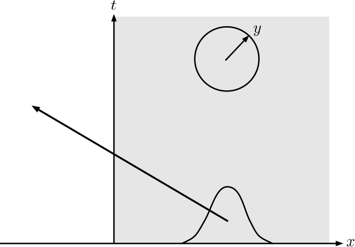
Figure 1: The arrival time problem defined using a model clock. The clock runs while the particle is in $x>0$.

For the moment we will assume only that the clock Hamiltonian is self adjoint, so that it may be written in the following form,

$$H_{c}=\int\ d\epsilon\ \epsilon\left|\epsilon\right>\left<\epsilon\right|$$ (11)

where the $\left|\epsilon\right>$ form an orthonormal basis for the Hilbert space of the clock. Later on we will restrict $H_{c}$ further by considering the accuracy of the clock. We will also quote some results for the special choice of $H_{c}=\hat{p}_{y}$, whose action is to simply shift the pointer position $y$ of the clock in proportion to time. This is the simplest and most frequently used choice for the clock Hamiltonian. The physical relevance of this and other clock models is discussed in Refs. clockchapter ; clock .

Our aim, for both arrival and dwell times, is to first solve for the evolution of the combined system of particle and clock. We write this as

$$\Psi(x,y,{\tau}) = \left<x,y\right|e^{-iH{\tau}}\left|\Psi_{0}\right>$$ (12)

$$= \left<x,y\right|\exp\left(-iH_{0}{\tau}-i{\lambda}\chi(\hat{x})H_{c}{\tau}\right)\left|\psi_{0}\right>\left|\phi_{0}\right>$$

$$= \int d\epsilon\left<y|\epsilon\right>\left<\epsilon|\phi_{0}\right>\left<x\right|\exp(-iH_{0}{\tau}-i{\lambda}\chi(\hat{x})\epsilon{\tau})\left|\psi_{0}\right>$$

and we then solve for the propagator in the integrand using path integral methods. We will take the total time ${\tau}$ to be sufficiently large that the wave packet has left the region defined by $\chi(x)$. We will then compute the final distribution of the pointer variable $y$, which is

$$\Pi(y)=\int_{-\infty}^{\infty}dx|\Psi(x,y,{\tau})|^{2}.$$ (13)

Our main aim is to show that the predictions of the clock model Eq.(13) reduce, in certain limits, to the standard forms described above.

I.4 Connections to Earlier Work

Clock models of the type Eq.(9) for arrival and dwell times have been studied by numerous previous authors, including Peres clock , Aharanov et al clock2 , Hartle Hartleclock and Mayato et al clockchapter . These studies are largely focused on the characteristics of clocks. Refs.clock ; clock2 are the works perhaps most closely related to the present work. They concentrate on the case of a clock Hamiltonian linear in momentum, with some elaborations on this basic model in the case of Ref.clock2 . Here, we focus on a different issue not addressed by these works, namely the dependence of the distribution Eq.(13) on the initial state of the particle, for reasonably general clock Hamiltonians. In particular, we determine the extent to which the standard semiclassical forms derived above are obtained for general initial states of the particle. We also use path integral methods to perform the calculations, in contrast to the scattering methods used in most of the previous works. Path integral methods similar to those employed here have previously been used in Refs. Sok ; Fer to explore the time taken to tunnel under a potential barrier, although these authors sought to define the tunneling time in terms of subsets of paths in the path integral, rather than by considering the behavior of a physical clock.

I.5 This Paper

The rest of this paper is arranged as follows. In Section II we review some path integral techniques and in particular the path decomposition expansion (PDX), which we will use to compute Eq.(12). We also introduce a useful semi-classical approximation. In Section III we compute Eqs.(12), (13) for the arrival time problem, and similarly in Section IV for the dwell time problem. We conclude in Section V.

II The path decomposition expansion and the semiclassical approximation

In this section we discuss the path decomposition expansion (PDX), which we shall make use of in the rest of this paper to calculate Eqs.(12),(13). We also introduce a useful semiclassical approximation, which significantly reduces the complexity of the calculations. Throughout this section we shall focus on the arrival time case, so that $\chi(x)=\theta(x)$.

To evaluate Eq.(12) we need to evaluate a propagator of the form

$$g(x_{1},\tau|x_{0},0)=\langle x_{1}|\exp\left(-i(H_{0}+V\theta(\hat{x}))\tau\right)|x_{0}\rangle,$$ (14)

for $x_{1}<0$ and $x_{0}>0$ (more general situations are considered in HaYe1 ). Here $V$ is some real number. This may be calculated using a sum over paths,

$$g(x_{1},\tau|x_{0},0)=\int{\cal D}x\exp\left(iS\right)$$ (15)

where

$$S=\int_{0}^{\tau}dt\left(\frac{1}{2}m\dot{x}^{2}-V\theta(x)\right),$$ (16)

and the sum is over all paths $x(t)$ from $x(0)=x_{0}$ to $x(\tau)=x_{1}$.

We can simplify the analysis by splitting off the sections of the paths lying entirely in $x>0$ or $x<0$. The way to do this is to use the path decomposition expansion PDX ; HaOr . Every path from $x_{0}>0$ to $x_{1}<0$ will typically cross $x=0$ many times, but all paths have a first crossing, at time $t$, say. As a consequence of this, it is possible to derive the formula,

$$g(x_{1},\tau|x_{0},0)=\frac{i}{2m}\int_{0}^{\tau}dtg(x_{1},\tau|0,t)\frac{\partial g_{r}}{\partial x}(x,t|x_{0},0)\big{|}_{x=0}$$ (17)

Here, $g_{r}(x,t|x_{0},0)$ is the restricted propagator obtained by a path integral of the form Eq.(15) summed over paths lying entirely in $x>0$. Its derivative at $x=0$ is given by a sum over all paths in $x>0$ which end on $x=0$ HaOr . Similar formulas may also be derived involving the last crossing time, and both the first and last crossings times PDX ; HaOr . The PDX is depicted in Figure (2).

Figure 2: The first crossing path decompositon expansion: paths from $x_{0}>0$ to $x_{1}<0$ consist of a restricted section of propagation to $x=0$, $(A)$, followed by unrestricted propagation along $x=0$ and to $x_{1}<0$ $(B)$.

Each element of these expressions can be calculated for a potential of the form $V\theta(x)$. The restricted propagator in $x>0$ is given by the method of images expression,

$$g_{r}(y,{\tau}|x,0)=\theta(y)\theta(x)\left(g_{f}(y,{\tau}|x,0)-g_{f}(-y,{\tau}|x,0)\right)e^{iV{\tau}},$$ (18)

where $g_{f}$ denotes the free particle propagator

$$g_{f}(y,{\tau}|x,0)=\left(\frac{m}{2\pi i{\tau}}\right)^{1/2}\exp\left(\frac{im(y-x)^{2}}{2{\tau}}\right).$$ (19)

Note that this means that

$$\left.\frac{\partial g_{r}}{\partial x}\right|_{x=0}=2\left.\frac{\partial g_{f}}{\partial x}\right|_{x=0},$$ (20)

and thus Eq.(17) can be written as,

$$\left<x_{1}\right|e^{-i(H_{0}+V\theta(\hat{x})){\tau}}\left|x_{0}\right>=\frac{1}{m}\int_{0}^{{\tau}}dt\left<x_{1}\right|e^{-i(H_{0}+V\theta(\hat{x}))({\tau}-t)}\delta(\hat{x})\hat{p}e^{-i(H_{0}+V)t}\left|x_{0}\right>,$$ (21)

where $\delta(\hat{x})=\left|0\right>\left<0\right|$ and $\left|0\right>$ denotes a position eigenstate $\left|x\right>$ at $x=0$.

The propagator from $x=0$ to $x_{1}>0$ is more difficult to calculate, because it will generally involve many re-crossings of the origin. This propagator may be calculated exactly by using the last crossing version of the PDX HaYe1 , but it may also be approximated using a semiclassical expression, which we now describe.

The exact propagator from the origin to a point $x_{1}<0$ consists of propagation along the edge of the potential followed by restricted propagation from $x=0$ to $x_{1}$. However, for sufficiently small $V$, we expect from the path integral representation of the propagator that the dominant contribution will come from paths in the neighbourhood of the straight line path from $x=0$ to $x_{1}<0$. These paths lie almost entirely in $x<0$, so we expect that the propagator may be approximated semiclassically by

$$\left<x_{1}\right|e^{-i(H_{0}+V\theta(\hat{x}))t}\left|0\right>\approx\left<x_{1}\right|e^{-iH_{0}t}\left|0\right>,$$ (22)

and thus Eq.(21) can be written as,

$$\left<x_{1}\right|e^{-i(H_{0}+V\theta(\hat{x})){\tau}}\left|x_{0}\right>\approx\frac{1}{m}\int_{0}^{{\tau}}dt\left<x_{1}\right|e^{-iH_{0}({\tau}-t)}\delta(\hat{x})\hat{p}e^{-i(H_{0}+V)t}\left|x_{0}\right>.$$ (23)

In Ref.HaYe1 it was shown that this semiclassical approximation holds for $E\gg V$, where $E$ is the kinetic energy of the particle.

III Arrival time distribution from an idealised clock

We now turn to the calculation of the arrival time distribution, Eq.(13), recorded by our model clock. Using the path decomposition expansion in the form Eq.(21) the state of the system Eq.(12) can be written as,

$$\Psi(x,y,{\tau}) = \left<x,y\right|e^{-i(H_{0}+{\lambda}\theta(\hat{x})H_{c}){\tau}}\left|\Psi_{0}\right>$$ (24)

$$= \frac{1}{m}\int d\epsilon\left<y|\epsilon\right>\left<\epsilon|\phi_{0}\right>$$

$$\times\int_{0}^{{\tau}}dt\left<x\right|\exp(-i(H_{0}+{\lambda}\epsilon\theta(\hat{x}))({\tau}-t))\delta(\hat{x})\hat{p}\exp(-i(H_{0}+{\lambda}\epsilon)t)\left|\psi_{0}\right>.$$

We can simplify this expression in two different regimes, the weak coupling regime of $E\gg{\lambda}\epsilon$, and the strong coupling regime of $E\ll{\lambda}\epsilon$.

III.1 Weak Coupling Regime

In the limit $E\gg{\lambda}\epsilon$ we can make use of the semiclassical approximation to the PDX formula, Eq.(23). This yields,

$$\Psi(x,y,{\tau}) = \frac{1}{m}\int d\epsilon\left<y|\epsilon\right>\left<\epsilon|\phi_{0}\right>$$ (25)

$$\times\int_{0}^{{\tau}}dt\left<x\right|\exp(-iH_{0}({\tau}-t))\delta(\hat{x})\hat{p}\exp(-i(H_{0}+{\lambda}\epsilon)t)\left|\psi_{0}\right>.$$

This means that the arrival time distribution is

$$\Pi(y) = \frac{1}{m^{2}}\int d\epsilon d\epsilon^{\prime}\left<\phi_{0}|\epsilon^{\prime}\right>\left<\epsilon^{\prime}|y\right>\left<y|\epsilon\right>\left<\epsilon|\phi_{0}\right>$$ (26)

$$\times\int_{0}^{{\tau}}dtdt^{\prime}\left<\psi_{0}\right|\exp(i(H_{0}+{\lambda}\epsilon^{\prime})t^{\prime})\hat{p}\delta(\hat{x})\exp(-iH_{0}(t^{\prime}-t))\delta(\hat{x})$$

$$\times\hat{p}\exp(-i(H_{0}+{\lambda}\epsilon)t)\left|\psi_{0}\right>$$

(Recall that we are assuming ${\tau}$ is sufficiently large that all the wavepacket is in $x<0$ at the final time, see the discussion below Eq.(12).) To proceed, we first note that for any operator $\hat{A}$, we have

$$\delta(\hat{x})\hat{A}\delta(\hat{x})=\delta(\hat{x})\left<0\right|\hat{A}\left|0\right>.$$ (27)

Using this in Eq.(26) gives,

$$\Pi(y) = \frac{1}{m^{2}}\int d\epsilon d\epsilon^{\prime}\left<\phi_{0}|\epsilon^{\prime}\right>\left<\epsilon^{\prime}|y\right>\left<y|\epsilon\right>\left<\epsilon|\phi_{0}\right>$$ (28)

$$\times\int_{0}^{{\tau}}dtdt^{\prime}\left<\psi_{0}\right|\exp(i(H_{0}+{\lambda}\epsilon^{\prime})t^{\prime})\hat{p}\delta(\hat{x})\hat{p}\exp(-i(H_{0}+{\lambda}\epsilon)t)\left|\psi_{0}\right>$$

$$\times\left<0\right|\exp(-iH_{0}(t^{\prime}-t))\left|0\right>.$$

We see here the appearance of the combination $\hat{p}\delta(\hat{x})\hat{p}$, and the main challenge is to show how this turns into the current operator, $\delta(\hat{x})\hat{p}+\hat{p}\delta(\hat{x})$.

Next we rewrite the integrals using

$$\int_{0}^{{\tau}}dtdt^{\prime}=\int_{0}^{{\tau}}dt\int_{t}^{{\tau}}dt^{\prime}+\int_{0}^{{\tau}}dt^{\prime}\int_{t^{\prime}}^{{\tau}}dt.$$ (29)

In the first term we set $u=t$, $v=t^{\prime}-t$, and in the second we set $u=t^{\prime}$, $v=t-t^{\prime}$ to obtain,

$$\Pi(y) = \frac{1}{m^{2}}\int d\epsilon d\epsilon^{\prime}\left<\phi_{0}|\epsilon^{\prime}\right>\left<\epsilon^{\prime}|y\right>\left<y|\epsilon\right>\left<\epsilon|\phi_{0}\right>\int_{0}^{{\tau}}du\int_{0}^{{\tau}-u}dv$$

$$\times\left\{\left<\psi_{0}\right|\exp(i(H_{0}+{\lambda}\epsilon^{\prime})u)\hat{p}\delta(\hat{x})\hat{p}\exp(-i(H_{0}+{\lambda}\epsilon)(u+v))\left|\psi_{0}\right>\left<0\right|\exp(iH_{0}v)\left|0\right>\right.$$

$$\left.+\left<\psi_{0}\right|\exp(i(H_{0}+{\lambda}\epsilon^{\prime})(u+v))\hat{p}\delta(\hat{x})\hat{p}\exp(-i(H_{0}+{\lambda}\epsilon)u)\left|\psi_{0}\right>\left<0\right|\exp(-iH_{0}v)\left|0\right>\right\}$$

Since we take the time ${\tau}$ to be large, we can extend the upper limits of the integrals to infinity. The integral over $v$ can then be carried out, to give,

$$\Pi(y) = \int d\epsilon d\epsilon^{\prime}\left<\phi_{0}|\epsilon^{\prime}\right>\left<\epsilon^{\prime}|y\right>\left<y|\epsilon\right>\left<h|\phi_{0}\right>$$

$$\times\frac{(-1)}{2m}\int_{0}^{\infty}du\left<\psi_{u}\right|e^{i{\lambda}\epsilon^{\prime}u}\big{(}\hat{p}\delta(\hat{x})+\delta(\hat{x})\hat{p}\big{)}e^{-i{\lambda}\epsilon u}\left|\psi_{u}\right>$$

$$\Pi(y) = \frac{(-1)}{2m}\int_{0}^{\infty}du|\Phi(y,u)|^{2}\left<\psi_{u}\right|\big{(}\hat{p}\delta(\hat{x})+\delta(\hat{x})\hat{p}\big{)}\left|\psi_{u}\right>$$ (31)

$$= \int_{0}^{\infty}dt|\Phi(y,t)|^{2}J(t)$$

where

$$\Phi(y,t)=\int d\epsilon\left<y|\epsilon\right>\left<\epsilon|\phi_{0}\right>e^{-i{\lambda}\epsilon t}=\left<y\right|e^{-i\lambda H_{c}t}\left|\phi_{0}\right>$$ (32)

is the wavefunction of the clock, and $J(t)$ is the current, Eq.(1).

This form shows that, in the weak coupling limit, our arrival time probability distribution yields the current, but smeared with a function depending on the clock state. We thus get agreement with the expected result, Eq.(7). Note that the physical quantity measured, the current, is not affected by the form of the clock Hamiltonian.

Although the form Eq.(31) holds for a wide class of clock Hamiltonians, not all choices make for equally good clocks. To further restrict the coupling $H_{c}$ we require that different arrival times may be distinguished up to some accuracy $\delta t$. For this to be the case we require that the clock wavefunctions corresponding to different arrival times are approximately orthogonal, so that

$$\int dy\Phi^{*}(y,t^{\prime})\Phi(y,t)\approx\begin{cases}1&\mbox{ if }t\approx t^{\prime}\\ 0&\mbox{ otherwise}\end{cases}$$ (33)

We easily see that,

$$\int dy\Phi^{*}(y,t^{\prime})\Phi(y,t) = \int d\epsilon d\epsilon^{\prime}dy\left<\phi_{0}|\epsilon^{\prime}\right>\left<\epsilon^{\prime}|y\right>\left<y|\epsilon\right>\left<\epsilon|\phi_{0}\right>e^{i{\lambda}(t^{\prime}\epsilon^{\prime}-t\epsilon)}$$ (34)

$$= \int d\epsilon|\phi_{0}(\epsilon)|^{2}e^{-i{\lambda}\epsilon\delta t}$$

where $\delta t=t-t^{\prime}$. Clearly this expression is equal to 1 if $\delta t=0$. Suppose now that $|\phi_{0}(\epsilon)|^{2}$ is peaked around some value $\epsilon_{0}$ with width $\sigma_{\epsilon}$. This integral will approximately vanish if

$${\lambda}\sigma_{\epsilon}\delta t>>1,$$ (35)

and so the resolution of the clock is given by $1/{\lambda}\sigma_{\epsilon}$. The relationship between $t$ and the pointer variable $y$ will depend on the specific model. It is easily seen that a clock with good characteristics may be obtained using, for example, a free particle with a Gaussian initial state. But clocks with more general Hamiltonians can also be useful if they evolve an initial Gaussian along an approximately classical path (as many Hamiltonians do). See Refs.clock ; clock2 ; Hartleclock ; clockchapter for further discussion of clock characteristics.

For the special case $H_{c}=\hat{p}_{y}$, $\left|\epsilon\right>=\left|p_{y}\right>$, the expression for the arrival time distribution simplifies, since

$$\Phi(y,t)=\int\frac{dp_{y}}{\sqrt{2\pi}}e^{ip_{y}(y-{\lambda}t)}\tilde{\phi}_{0}(p_{y})=\phi_{0}(y-{\lambda}t)$$ (36)

The time is related to $y$ by $t=y/\lambda$ and the expected form Eq.(7) then becomes a simple convolution.

III.2 Strong Coupling Regime

III.2.1 Special Case: $H_{c}=\hat{p}_{y}$

We now turn to the limit of strong coupling between the particle and clock. The analysis of the case of general clock Hamiltonian is rather subtle, so before we tackle this we first examine the special case where the clock Hamiltonian is linear in the momentum. That is, we have,

$$H_{c}=\hat{p}_{y}=\int dp_{y}\;p_{y}\left|p_{y}\right>\left<p_{y}\right|.$$ (37)

We start from Eq.(24), and insert a complete set of momentum states for the particle, $p$ to obtain,

$$\Psi(x,y,{\tau}) = \frac{1}{m}\int\frac{dp_{y}dp}{\sqrt{2\pi}}\left<y|p_{y}\right>\tilde{\phi}_{0}(p_{y})\exp(-i(E+{\lambda}p_{y}){\tau})p\left<p|\psi_{0}\right>$$

$$\times\int_{0}^{{\tau}}dt\left<x\right|\exp(-i(H_{0}-{\lambda}p_{y}\theta(-\hat{x}))t)\left|0\right>\exp(iEt),$$

where $\tilde{\phi}_{0}(p_{y})$ is the initial momentum space wavefunction of the clock, and $E=p^{2}/2m$ is the kinetic energy of the particle. Note the appearance of the momentum $p$ in the integrand. The expression involving the integral over $t$ has been computed previously using the final crossing PDX Hal2 ; HaYe1 . In the limit ${\tau}\to\infty$ it is given by,

$$\int_{0}^{\infty}dt\left<x\right|\exp(-i(H_{0}-{\lambda}p_{y}\theta(-\hat{x}))t)\left|0\right>\exp(iEt) = \sqrt{\frac{2m}{{\lambda}p_{y}}}\exp\left(-ix\sqrt{2m(E+{\lambda}p_{y})}\right).$$

We can now write our probability distribution for $y$. Carrying out the $x$ integral we obtain,

$$\Pi(y) = \int dp_{y}dp_{y}^{\prime}dpdp^{\prime}\tilde{\phi}_{0}^{*}(p_{y}^{\prime})\tilde{\phi}_{0}(p_{y})\left<p_{y}^{\prime}|y\right>\left<y|p_{y}\right>\exp(-i{\lambda}(p_{y}-p_{y}^{\prime}){\tau})$$

$$\times\frac{pp^{\prime}}{m}\left<\psi_{0}|p^{\prime}\right>\left<p|\psi_{0}\right>\exp(-i(E-E^{\prime}){\tau})$$

$$\times\frac{2}{\sqrt{{\lambda}^{2}p_{y}p_{y}^{\prime}}}\delta\left(\sqrt{2m(E+{\lambda}p_{y})}-\sqrt{2m(E^{\prime}+{\lambda}p_{y}^{\prime})}\right).$$

Using the formula $\delta(f(x))=\delta(x)/f^{\prime}(0)$, we can carry out the $p_{y}^{\prime}$ integral to give,

$$\Pi(y) \approx \int dp_{y}dpdp^{\prime}|\tilde{\phi}_{0}(p_{y})|^{2}\frac{pp^{\prime}}{m^{2}}\left<\psi_{0}|p^{\prime}\right>\left<p|\psi_{0}\right>\exp\left(-i\frac{(E-E^{\prime})}{{\lambda}}y\right)\frac{2}{{\lambda}}\sqrt{\frac{2m}{{\lambda}p_{y}}}$$

$$= \int dp_{y}|\tilde{\phi}_{0}(p_{y})|^{2}\frac{2}{m^{2}}\sqrt{\frac{2m}{{\lambda}p_{y}}}\left<\psi_{0}\right|\exp\left(iH_{0}\frac{y}{{\lambda}}\right)\hat{p}\delta(\hat{x})\hat{p}\exp\left(-iH_{0}\frac{y}{{\lambda}}\right)\left|\psi_{0}\right>$$

$$= A\left<\psi_{0}\right|\exp\left(iH_{0}\frac{y}{{\lambda}}\right)\hat{p}\delta(\hat{x})\hat{p}\exp\left(-iH_{0}\frac{y}{{\lambda}}\right)\left|\psi_{0}\right>$$ (41)

where $A$ is some constant whose explicit form is not required and we have used the fact that $E<<{\lambda}p_{y}$ to approximate,

$$\phi\left(p_{y}+\frac{E-E^{\prime}}{{\lambda}}\right)\approx\phi(p_{y}).$$ (42)

We see therefore that in this limit the probability of finding the clock at a position $y$ is given by the kinetic energy density of the system at the time $t=y/{\lambda}$, in agreement with Eqs.(2) and (3).

Note that there is no response function involved in this case, as one might have expected from the general form Eq.(7). A similar feature was noted in the complex potential model of Ref.Hal2 ). It seems likely that this is because the strong measurement prevents the particle from leaving $x>0$ until the last moment, so that the response function $R(t,s)$ is effectively a delta-function concentrated around the latest time.

III.2.2 General Case

As well as the approximations valid for $E<<{\lambda}p_{y}$, the key to the analysis in the special case presented above is that the position space eigenfunction of the clock Hamiltonian with eigenvalue $p_{y}$ takes the simple form,

$$\left<y|p_{y}\right>=\frac{1}{\sqrt{2\pi}}\exp(iyp_{y}).$$ (43)

This greatly simplifies the resulting calculation. For the case of a more general clock Hamiltonian, the eigenstates will not have this simple form. Instead we make a standard WKB approximation for the eigenstates of the clock,

$$\left<y|\epsilon\right>=C(y,\epsilon)\exp(iS(y,\epsilon))$$ (44)

where $S(y,\epsilon)$ is the Hamilton Jacobi function of the clock at fixed energy. This means Eq.(III.2.1) becomes,

$$\Pi(y) \approx \int d\epsilon dpdp^{\prime}|\left<\epsilon|\phi_{0}\right>|^{2}\frac{pp^{\prime}}{m^{2}}\left<\psi_{0}|p^{\prime}\right>\left<p|\psi_{0}\right>\left<\epsilon+\frac{(E-E^{\prime})}{{\lambda}}|y\right>\left<y|\epsilon\right>\frac{2}{{\lambda}}\sqrt{\frac{2m}{{\lambda}\epsilon}}$$ (45)

$$\approx \int d\epsilon|\left<\epsilon|\phi_{0}\right>|^{2}\frac{2}{m^{2}}\sqrt{\frac{2m}{{\lambda}\epsilon}}|C(y,\epsilon)|^{2}$$

$$\times\left<\psi_{0}\right|\exp\left(iH_{0}\frac{1}{{\lambda}}\frac{\partial S(y,\epsilon)}{\partial\epsilon}\right)\hat{p}\delta(\hat{x})\hat{p}\exp\left(-iH_{0}\frac{1}{{\lambda}}\frac{\partial S(y,\epsilon)}{\partial\epsilon}\right)\left|\psi_{0}\right>$$

where we have used,

$$\left<\epsilon+\frac{(E-E^{\prime})}{{\lambda}}|y\right>\left<y|\epsilon\right>\approx|C(y,\epsilon)|^{2}\exp\left(-i\frac{(E-E^{\prime})}{{\lambda}}\frac{\partial S(y,\epsilon)}{\partial\epsilon}\right),$$ (46)

which is valid for $E-E^{\prime}<<{\lambda}\epsilon$.

We now suppose that the clock state is a simple Gaussian in $y$, or equivalently in $p_{y}$. It follows that it will be peaked in $\epsilon$ about some value $\epsilon_{0}$. This means that the integral over $\epsilon_{0}$ in Eq.(45) may be carried out. The result for $\Pi(t)$ will again be proportional to the kinetic energy density, of the form Eq.(2), where the relationship between $t$ and the pointer variable $y$ is defined by the equation

$$t=\frac{1}{{\lambda}}\frac{\partial S(y,\epsilon_{0})}{\partial\epsilon}$$ (47)

as one might expect from Hamilton-Jacobi theory Goldstein . Hence the arrival time distribution has the expected general form, Eq.(2) (and therefore Eq.(3) also holds), but the precise definition of the time variable depends on the properties of the clock.

IV Dwell Times

We now turn to the related issue of dwell times. Here the aim is to measure the time spent by the particle in a given region of space which, for simplicity, we take to be the region $[-L,L]$. This is portrayed in Figure (3). In this section we will work exclusively in the weak coupling regime where $E>>{\lambda}\epsilon$.

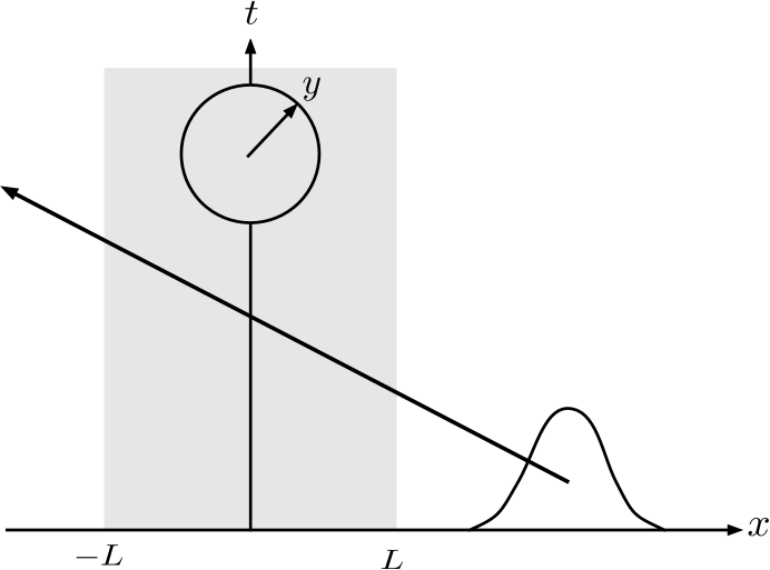
Figure 3: The dwell time problem, defined using a model clock. The clock runs while the particle is in the region $[-L,L]$.

The starting point is the final state of the particle plus clock, Eq.(12), which we write as

$$\Psi(x,y,\tau)=\left<x,y\right|e^{-i(H_{0}+{\lambda}H_{c}\chi(\hat{x})){\tau}}\left|\Psi_{0}\right>.$$ (48)

where $\chi(\hat{x})=\theta(\hat{x}+L)\theta(L-\hat{x})$. We wish to re-express this using the path decomposition in a similar way to Eq.(24). For this case we need a PDX which is more general than the one used for the arrival time, since there are now crossings of two surfaces. One way to proceed is to use the path integral expression for the first crossing of $x=L$ and $x=-L$, which is

$$\Psi(x,y,\tau) = \frac{1}{m^{2}}\int d\epsilon\left<\epsilon|\phi_{0}\right>\left<y|\epsilon\right>\int_{0}^{\infty}ds\int_{-\infty}^{{\tau}-s}dt\left<x\right|\exp(-i(H_{0}+{\lambda}\chi(\hat{x})\epsilon)({\tau}-s-t))\left|-L\right>$$ (49)

$$\left<-L\right|\hat{p}\exp(-i(H_{0}+{\lambda}\chi(\hat{x})\epsilon)s)\left|L\right>\left<L\right|\hat{p}\exp(-iH_{0}t)\left|\psi_{0}\right>,$$

This is shown in Figure (4).

Figure 4: The PDX used for the dwell time problem: Paths from $x_{0}>0$ to $x_{1}<0$ have a first crossing of $x=L$ at a time $t$ and a first crossing of $x=-L$ at a time $t+s$.

However there are other choices we could make. We could consider the first crossing of $x=L$ and the last crossing of $x=-L$ for example. In the semiclassical limit these choices lead to equivalent expressions for the dwell time. It would be interesting to explore what differences do arise in other regimes. This will be addressed elsewhere.

It will prove more useful to work with the wavefunction in position space for the clock and momentum space for the particle. Changing to this representation, and making use of the semiclassical approximation, Eq.(23), we obtain,

$$\left<p,y|\Psi_{{\tau}}\right> \approx \frac{1}{m^{2}}\int d\epsilon\left<y|\epsilon\right>\left<\epsilon|\phi_{0}\right>\int_{0}^{\infty}ds\int_{-\infty}^{{\tau}-s}dt\left<p\right|\exp(-iH_{0}({\tau}-s-t))\left|-L\right>$$ (50)

$$\times \left<-L\right|\hat{p}\exp(-i(H_{0}+{\lambda}\epsilon)s)\left|L\right>\left<L\right|\hat{p}\exp(-iH_{0}t)\left|\psi_{0}\right>$$

This is a semiclassical version of the PDX for first crossing of $x=L$ and $x=-L$. Now we make the standard scattering approximation of letting the upper limit of the integral over $t$ go to infinity. This means we can carry out the $t$ and $s$ integrals to obtain,

$$\left<p,y|\Psi_{{\tau}}\right> \approx \int d\epsilon\left<y|\epsilon\right>\left<\epsilon|\phi_{0}\right>\exp(-iE{\tau})\exp(-i2Lm{\lambda}\epsilon/|p|)\left<p|\psi_{0}\right>,$$ (51)

where we have used the standard integral HaYe1 ,

$$\int_{0}^{\infty}ds\left<x\right|\exp(-iH_{0}s)\hat{p}\left|0\right>e^{iEs}=m\exp(i|x|\sqrt{2mE})$$ (52)

and

$$\int_{-\infty}^{\infty}\frac{dt}{2\pi}\left<x\right|\hat{p}\exp(-i(H_{0}-E)t)\left|\psi_{0}\right>=\left<x\right|\hat{p}\delta(H_{0}-E)\left|\psi_{0}\right>=m\left<x\right|\delta(\hat{p}-p)\left|\psi_{0}\right>$$ (53)

Here, we have neglected the term involving $\delta(\hat{p}+p)$ since this corresponds to reflection, which will be negligible in this semiclassical limit. We have also use the fact that $E\gg{\lambda}\epsilon$ to approximate,

$$\exp\left(i2L\sqrt{2m(E-{\lambda}\epsilon)}\right)\approx\exp\left(i2L|p|-i2Lm{\lambda}\epsilon/|p|\right).$$ (54)

We therefore obtain the distribution for $y$ as,

$$\Pi(y) = \int dp\left|\left<p,y|\Psi_{{\tau}}\right>\right|^{2}$$ (55)

$$= \int d\epsilon d\epsilon^{\prime}\left<\phi_{0}|\epsilon^{\prime}\right>\left<\epsilon^{\prime}|y\right>\left<y|\epsilon\right>\left<\epsilon|\phi_{0}\right>\int dp|\psi_{0}(p)|^{2}\exp\left(\frac{i2Lm{\lambda}}{|p|}(\epsilon^{\prime}-\epsilon)\right)$$

$$= \int dp|\psi_{0}(p)|^{2}|\Phi(y,2Lm/|p|)|^{2}$$

where,

$$\Phi(y,2Lm/|p|) = \int d\epsilon\left<y|\epsilon\right>\left<\epsilon|\phi_{0}\right>\exp\left(\frac{-i2Lm{\lambda}}{|p|}\epsilon\right)$$ (56)

$$= \left<y\right|\exp\left(\frac{-i2Lm{\lambda}}{|p|}H_{c}\right)\left|\phi_{0}\right>$$

is the clock wavefunction. We may rewrite this as

$$\Pi(y)=\int dt\ |\Phi(y,t)|^{2}\langle\psi_{0}|\delta\left(t-\frac{2mL}{|\hat{p}|}\right)|\psi_{0}\rangle$$ (57)

It is therefore of precisely the desired form, Eqs.(6), (7), with $|\Phi(y,t)|^{2}$ playing the role of the response function. The discussion of clock characteristics is then exactly the same as the arrival time case discussed in Section 3.

V Conclusion

We have studied the arrival and dwell time problems defined using a model clock with a reasonably general Hamiltonian. We found that in the limit of weak particle-clock coupling, the time of arrival probability distribution is given by the probability current density Eq.(1), smeared with some function depending on the initial clock wave function, Eq.(7). This is expected semiclassically, agrees with previous studies and is independent the precise form of the clock Hamiltonian.

In the regime of strong coupling, we found that the arrival time distribution is proportional to the kinetic energy density of the particle, in agreement with earlier approaches using a complex potential. The fact that two very different models give the same result in this regime suggests that the form Eq.(3) is the generic result in this regime, independent of the method of measurement. It would be of interest to develop a general argument to prove this. (See Ref.ech for further discussion of this regime).

For the case of dwell time, we have shown that the dwell time distribution measured by our model clock may be written in terms of the dwell time operator in semiclassical form, smeared with some convolution function, Eqs.(6), (7).

In all of these cases, the precise form of the clock Hamiltonian and clock initial state determine the relationship between time $t$ and the pointer variable $y$ and they determine the form of the response function $R$ in the general form Eq.(7). These are particularly simple for the special case $H_{C}=\hat{p}_{y}$ explored previously. However, what is important is that, once the definition of the time variable is fixed, the clock characteristics do not effect the form of the underlying distributions – the $\Pi(s)$ in Eq.(7). The $\Pi(s)$ are always one of the general forms Eqs.(1), (2) and (6), no matter what the clock characteristics are. This means that these general forms will always play central role, irrespective of how they are measured.

References

- (1) J.G.Muga, R.Sala Mayato and I.L.Egusquiza (eds), Time in Quantum Mechanics (Springer, Berlin, 2002).
- (2) J.G. Muga, A. Ruschhaupt and A. del Campo (eds), Time in Quantum Mechanics - Vol. 2 (Springer, Berlin, 2010).
- (3) J.G.Muga and C.R.Leavens, Phys.Rep. 338, 353 (2000).
- (4) G.R.Allcock, Ann.Phys 53, 253 (1969); 53, 286 (1969); 53, 311 (1969).
- (5) J. G. Muga, J. P. Palao and C. R. Leavens Phys. Lett. A 253, 21 (1999).
- (6) J.J.Halliwell and J.M.Yearsley, Phys. Rev. A 79, 062101 (2009); Phys. Lett. A374, 154-157 (2009).
- (7) A.J.Bracken and G.F.Melloy, J.Phys. A27, 2197 (1994); S.P.Eveson, C.J.Fewster and R.Verch, Ann.Inst. H.Poincaré 6, 1 (2005); M.Penz, G.Grübl, S.Kreidl and P.Wagner, J.Phys. A39, 423 (2006); M.V.Berry, J.Phys. A43, 1 (2010).
- (8) B.Misra and E.C.G.Sudarshan, J.Math.Phys. 18, 756 (1977); A. Peres, Am. J. Phys. 48, 931 (1980).
- (9) J.Echanobe, A. del Campo and J.G.Muga, Phys. Rev. A 77, 032112 (2008).
- (10) J.J.Halliwell, Phys. Rev. A77, 062103 (2008).
- (11) J.G.Muga, D.Seidel and G.C.Hegerfeldt, J.Chem.Phys. 122, 154106 (2005).
- (12) Jose Munoz, Inigo L.Egusquiza, Adolfo del Campo, Dirk Seidel and J.Gonzalo Muga, Chapter 5 of Ref.time2 .
- (13) A.Peres, Am. J. Phys. 48, 552 (1980); Quantum Theory: Concepts and Methods (Kluwer Academic, Dordrecht, 1993).
- (14) R.S.Mayato, D.Alonso & I.L.Egusquiza, Chapter 8 of Ref.time .
- (15) Y.Aharonov, J.Oppenheim, S.Popescu, B.Reznik and W.G.Unruh, Phys. Rev. A57, 4130 (1998).
- (16) J.B.Hartle, Phys. Rev. D 38, 2985 (1988).
- (17) D. Sokolovski and J.N.L Connor, Sol. Stat. Comm., 89, 475 (1994); Phys. Rev. A, 44, 1500 (1991).
- (18) H.A. Fertig, Phys. Rev. Lett., 65, 2321 (1990).
- (19) A.Auerbach and S.Kivelson, Nucl.Phys. B257, 799 (1985); P. van Baal, in Lectures on Path Integration, edited by H.A. Cerdeira et al. (World Scientific, Singapore, 1993); J.J.Halliwell, Phys.Lett. A207, 237 (1995).
- (20) J.J.Halliwell and M.E.Ortiz, Phys.Rev. D48, 748 (1993).
- (21) H.Goldstein, Classical Mechanics (Addison Wesley, Reading, MA, 1980).