Relaxation time ansatz and shear and bulk viscosities of gluon matter

Abstract

Shear and bulk viscosity-to-entropy density ratios are calculated for pure gluon matter in a nonequilibrium mean-field quasiparticle approach within the relaxation time approximation. We study how different approximations used in the literature affect the results for the shear and bulk viscosities. Though the results for the shear viscosity turned out to be quite robust, all evaluations of the shear and bulk viscosities obtained in the framework of the relaxation time approximation can be considered only as rough estimations.

I Introduction

High-energy heavy-ion collisions at RHIC and LHC energies have shown evidence for a new state of matter characterized by very low shear viscosity to entropy density ratio, $\eta/s$, similar to a nearly ideal fluid (see  Romatschke ; Aamodt ). Lattice calculations indicate that the crossover region between hadron and quark-gluon matter has been reached in these experiments. On the other hand, for the pure gluon ${\rm SU}(3)$ theory lattice calculations demonstrate the occurrence of the first-order phase transition (see BEG95 ; Pa09 ). Recently, there appeared gluon lattice data on ratios of the shear SN07 ; Ma07 and bulk Me08 ; SN07 viscosity to the entropy density.

Among various existing phenomenological approaches, quasiparticle models are used to reproduce results obtained in the lattice QCD (see PKPS96 ; PC05 ; IST_05 ; KTV09 ; KTV10 ). In the case of gluodynamics, quasiparticle models rely on the assumption that for a temperature $T$ below the critical one, $T<T_{c}$, the system consists of a gas of massive glueballs and, for $T>T_{c}$, the system consists of deconfined gluons. Perturbative estimates of the shear and bulk viscosities in gluodynamics were performed in NS05 ; Me08 ; CDDW and nonperturbative evaluations were made in BKR09 ; KTVglue1 ; BKR10 ; DA within the quasiparticle models with temperature-dependent masses in the relaxation time approximation with some additional ansatze resulting in essentially different expressions for the bulk viscosities.

Here we continue to exploit the mean-field-based quasiparticle model with parameters fitted in KTVglue1 to fulfill the modern lattice data. Using two possible ansatze for the collision term in the relaxation time approximation we derive expressions for the shear and bulk viscosities to entropy density ratios for the pure gluon ${\rm SU}(3)$ theory at $T>T_{c}$ and compare the results with the lattice data. Our results demonstrate ambiguities in calculation of the bulk viscosity within the relaxation time approach.

II The quasiparticle model

We start with the expression for the gluon energy-momentum density tensor in a relativistic mean-field model,

$$T^{\mu\nu}=\int d\Gamma\,\frac{p^{\mu}p^{\nu}}{E}f(t,\vec{r};E,\vec{p})+g^{\mu\nu}B[m^{2}(\varphi)]~{},$$ (1)

obeying the conservation law

$$\partial_{\mu}T^{\mu\nu}=0.$$ (2)

Here

$$d\Gamma = d_{g}\frac{d^{3}{p}}{(2\pi)^{3}}~{},\quad p^{\mu}=\left\{E[m^{2}(\varphi)],\vec{p}\right\}~{},$$

for gluons with a degeneracy factor $d_{g}=2(N^{2}_{c}-1)=16$, $N_{c}=3$; $\varphi$ is a mean field; summation over the repeated indices is implied. In this model the quasiparticle energy is given by

$$E=\sqrt{\vec{p}^{\,\,2}+m^{2}(\varphi)}~{}.$$ (3)

We assume that the quasiparticle distribution function $f$ obeys the kinetic equation

$$E^{-1}p^{\mu}\partial_{\mu}f-\nabla E\nabla_{\vec{p}}f = \mbox{St}f,$$ (4)

where $\mbox{St}f$ is the collision term satisfying the condition

$$\int d\Gamma E\ \mbox{St}f=0.$$ (5)

Applying (2) for $\nu=0$ and using (1) and (5) we derive the consistency condition for the effective bag constant

$$\frac{dB}{d\varphi} = -\frac{dm}{d\varphi}\rho_{s},$$ (6)

where

$$\rho_{s}=\int d\Gamma\,\frac{m}{E}\,f\,$$ (7)

is the scalar density. Note that in these expressions the quasiparticle energy is a functional of the distribution function $E=E[f]$. In thermal equilibrium relation (6) coincides with the thermodynamical consistency condition derived in GY95 and used in the model KTVglue1 .

The local equilibrium distribution function for a gluon is

$$f^{\rm l.eq.}(p^{\mu}_{\rm l.eq.},x^{\mu})=\left[e^{\frac{p^{\mu}_{\rm l.eq.}u_{\mu}(t,\vec{r})}{T(t,\vec{r})}}-1\right]^{-1}~{}.$$ (8)

Here $p^{\mu}_{\rm l.eq.}=(E^{\rm l.eq.},\vec{p})$,

$$E^{\rm l.eq.}=\sqrt{\vec{p}^{\,2}+m^{2}\{\varphi^{\rm l.eq.}[T(t,\vec{r})]\}},$$

and the four-velocity of the frame is $u^{\mu}\simeq[1,\vec{u}(t,\vec{r})]$ for $|\vec{u}|\ll 1$. Following KTVglue1 , we use the pole mass

$$(m^{\rm l.eq.})^{2}\equiv m^{2}[\varphi^{\rm l.eq.}(T)]=\frac{N_{c}}{6}\ g^{2}(T)\ T^{2}$$ (9)

as the gluon quasiparticle mass in local equilibrium. The temperature-dependent strong interaction coupling in the next to leading order is given by

$$g^{2}(T)=\frac{48\pi^{2}}{11N_{c}[\ln(\frac{\lambda(T-T_{s})}{T_{c}})^{2}+\frac{102}{121}\ln\ln(\frac{\lambda(T-T_{s})}{T_{c}})^{2}]}~{}.$$ (10)

All previous papers exploited $g^{2}$ up to the leading order using only the first term in the denominator of (10). In Ref. KTVglue1 , working within this leading order we fitted the parameters $\lambda$ and $T_{s}$ to fulfill the new lattice data Pa09 for the reduced pressure, energy, enthalpy and trace anomaly. However, we found that in the perturbative limit [at $\ln\ln(\frac{\lambda(T-T_{s})}{T_{c}})^{2}\gg 1$] the correction including the double-logarithmic term yields a larger contribution to $dm^{2}/dT^{2}$ than the leading logarithmic term. Since one of our aims in the given paper is to improve our fit in the perturbative limit, we keep the double-logarithmic correction and tune parameters to reproduce thermodynamic characteristics of the system. Our fit KTVglue1 with $g^{2}$ calculated up to leading order was performed with the parameters $T_{s}/T_{c}=0.5853$, $T_{c}=265$ MeV, and $\lambda=3.3$. The new fit with $g^{2}$ calculated up to subleading order yields $T_{s}/T_{c}=0.015$, $T_{c}=265$ MeV, and $\lambda=1.53$. Our previous fit of the reduced pressure, energy, enthalpy and trace anomaly KTVglue1 proves to be almost unchanged. Therefore, we do not redraw those figures here.

Generally, the running coupling constant $\alpha(T,r)=g^{2}(T,r)/(4\pi)$ depends on the temperature and distance and differs from the effective one determined as $\alpha(T)=g^{2}(T)/(4\pi)$ following Eq. (10). The quadratic rise of $\alpha(T=0,r)$ (see solid line in Fig. 6 of  Kaczmarek_07 ) is a nonperturbative effect that stems from the linear rising string tension term in the potential, while at small distances the logarithmic weakening of the coupling is visible and at sufficiently small distances it reaches the perturbative behavior (asymptotic freedom). At finite temperatures, $\alpha(T,r)$ follows this zero-temperature behavior to relatively large distances, before Debye screening sets in, leading to a maximum and a decrease at larger distances (see Fig. 6 of Ref. Kaczmarek_07 ). The value $\alpha$ is a temperature-dependent coupling constant determined with the help of the Debye screened potential at large distances  Kaczmarek_07 . Thus, the behavior at large distances of the coupling, which one may use to calculate thermodynamical characteristics in quasiparticle models, is not defined uniquely. Therefore, in Fig. 1 along with the effective running coupling constant $\alpha$ (circles) the coupling constant $\alpha_{max}$ (squares) is plotted to be defined by the maximum in $\alpha(T,r)$ Kaczmarek_07 . As can be seen, both estimates of the running constant noticeably differ near the critical temperature and tend to coincide at high temperatures. In Fig. 1, we demonstrate also that the running constant $\alpha(T)$ calculated up to the next to leading order with the help of Eq. (10) in the given work (solid line) and those calculated up to the leading order with the parameters from KTVglue1 (dash-dotted line) and from BKR10 (dashed line) deviate only little from each other, describing reasonably the lattice data of Ref. Kaczmarek_07 . Note that the parametrization from Ref. BKR10 is fitted to the old lattice data on thermodynamical quantities and does not describe properly the new lattice data Pa09 .

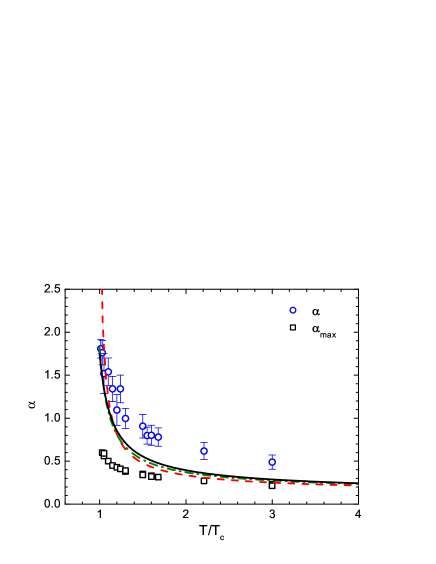
Figure 1: (Color online) The effective running coupling $\alpha(T)=g^{2}(T)/(4\pi)$ as a function of $T/T_{c}$. The points are the lattice data Kaczmarek_07 (see explanation in the text). The solid line is the result of our new fit (10). The dash-dotted line is our (leading-order) fit KTVglue1 . The dashed curve is the (leading-order) fit of Ref. BKR10 with $T_{s}/T_{c}=0.73$, $T_{c}=271$ MeV, and $\lambda=4.3$.

III Shear and bulk viscosities

We define the shear, $\eta$, and bulk, $\zeta$, viscosities as coefficients, entering into the variation of the energy-momentum tensor in the local rest frame:

$$\Delta T_{ij} = -\zeta\ \delta_{ij}{\vec{\nabla}}\cdot\vec{u}+\eta\ W_{ij},$$ (11)

$${\rm with}\quad W_{ij} = \partial_{i}u_{j}+\partial_{j}u_{i}+\frac{2}{3}\delta_{ij}\,{\vec{\nabla}}\cdot\vec{u}~{}.$$

Here Latin indices $1,2,3$ correspond to the spatial components. Summation over the repeated spatial indices is implied. To find the shear viscosity, $\eta$, we set $i\neq j$ in (11). To find the bulk viscosity, $\zeta$, we substitute $i=j$ in (11) and use the fact that $T_{ii}^{\rm l.eq}=3P^{\rm l.eq}$.

The operation $\Delta$ in (11) needs explanation. According to the work of Abrikosov and Khalatnikov AKh , in quasiparticle Fermi liquid theory one usually exploits the fact that the following combination enters into the original Landau collision term:

$$\delta\left(\sum_{a}E_{a}[f]\right)\cdot\left\{f(E_{1})f(E_{2})[1+f(E_{3})][1+f(E_{4})]\right.$$

$$\left.-f(E_{3})f(E_{4})[1+f(E_{1})][1+f(E_{2})]\right\},$$ (12)

where $E_{a}$ are the functionals of the exact nonequilibrium distribution function $f_{a}$ and $a=1,2,3,4$. The term in curly braces term is zero for $f^{\rm l.eq.}(E_{a})$ given by

$$f^{\rm l.eq.}(E)=\left[e^{\frac{p^{\mu}u_{\mu}(t,\vec{r})}{T(t,\vec{r})}}-1\right]^{-1}{\rm with}\,p^{\mu}=[E(\vec{p}),\vec{p}]\,,$$ (13)

where $E(\vec{p})$ is determined by Eqs. (3) and (6) and depends on the nonequilibrium distribution. Thus, ${\rm{St}}f^{\rm l.eq.}(E)=0$. However, following KTVglue1 the same collision term should vanish also for local equilibrium, i.e., $\mbox{St}f^{\rm l.eq.}(E^{\rm l.eq.})=0$. Let us demonstrate this by an example of the $2\rightarrow 2$ processes, as they are described by the four-momentum kinetic Kadanoff-Baym equation. Then the local collision term renders IKV2

$$C^{\rm loc.}=d^{2}\int\frac{d^{4}{p_{1}}}{(2\pi)^{4}}\frac{d^{4}{p_{2}}}{(2\pi)^{4}}\frac{d^{4}{p_{3}}}{(2\pi)^{4}}|M|^{2}$$

$$\times\delta^{4}\left(p+p_{1}-p_{2}-p_{3}\right)A(x,p)A(x,p_{1})A(x,p_{2})A(x,p_{3})$$

$$\times\left\{f(x,p_{2})f(x,p_{3})[1+f(x,p_{1})][1+f(x,p)]\right.$$

$$\left.-[1+f(x,p_{2})][1+f(x,p_{3})]f(x,p_{1})f(x,p)\right\},$$ (14)

where $M$ is the properly normalized matrix element and $A=-2\mbox{Im}G^{R}$ is the spectral function (density of states) that implicitly depends on the corresponding distribution function $f$, $G^{R}$ is the retarded Green function, and $p_{0}$ and $\vec{p}$ are independent variables. The Landau quasiparticle collision term is obtained from here provided one sets $A[f]=2\pi\delta[p_{0}^{2}-\vec{p}^{\,2}-m_{0}^{2}-\mbox{Re}\Sigma^{R}(p,[f])]$, where $m_{0}$ is the free particle mass and $\Sigma^{R}$ is the retarded self-energy. Here the local equilibrium distribution fulfills the relation

$$f^{\rm l.eq.}(x,p+q)[1+f^{\rm l.eq.}(x,p)]$$

$$=[f^{\rm l.eq.}(x,p)-f^{\rm l.eq.}(x,p+q)]f^{\rm l.eq.}(x,q),$$ (15)

where

$$f^{\rm l.eq.}(x,p)=\left[\exp\left(\frac{p^{\mu}u_{\mu}(t,\vec{r})}{T(t,\vec{r})}\right)-1\right]^{-1},$$ (16)

i.e., in contrast to (8) and (13), $p_{0}$ and $\vec{p}$ are independent variables. With the help of this relation we can see that the term in the curly braces in (III) is zero independently of values of $A$. Thus, $C^{\rm loc.}=0$ for two distributions: $F\equiv iG^{-+}=A[f^{\rm l.eq.}]f^{\rm l.eq.}$ and $F=A[f]f^{\rm l.eq.}$ (whereas the real solution of the kinetic equation is $F=A[f]f$). In our model $m$ does not depend on $p$, and the Landau quasiparticle collision term is obtained provided one sets in (III) $A[f^{\rm l.eq.}]=(\pi/E^{\rm l.eq.})\delta(p_{0}-E^{\rm l.eq.})$ (or $A[f]=(\pi/E[f])\delta(p_{0}-E[f])$). Note that in the Landau quasiparticle kinetics one neglects memory effects; therefore, we indeed may use the local approximation in Eq. (III).

Then, returning to our quasiparticle model we can expand the distribution function near $f^{\rm l.eq.}(E^{\rm l.eq.})$, i.e. (8), performing variations as

$$\delta f = f(E)-f^{\rm l.eq.}(E^{\rm l.eq.}),$$ (17)

$$\delta T^{\mu\nu} = T^{\mu\nu}[f(E)]-T^{\mu\nu}[f^{\rm l.eq}(E^{\rm l.eq.})]\,,$$

i.e., with $\Delta=\delta$ in Eq. (11), and alternatively we can introduce the operation $\Delta$ as $\Delta=\widetilde{\delta}$, where

$$\widetilde{\delta}{f} = f(E[f])-f^{\rm l.eq.}(E[f]),$$ (18)

$$\widetilde{\delta}T^{\mu\nu} = T^{\mu\nu}[f(E)]-T^{\mu\nu}[f^{\rm l.eq}(E)]\,,$$

where $f^{\rm l.eq.}(E[f])$ is given by Eq. (13). Subtracting (17) from (18) we obtain the relation

$$\widetilde{\delta}f={\delta}f-\left(\frac{\partial f}{\partial E}\right)^{\rm l.eq.}\delta E\,.$$ (19)

Below we use both possible choices of the $\Delta$ operation.

Performing variations in (1) we find

$$\Delta T_{ij}=\int d\Gamma\frac{p_{i}p_{j}}{E}\Delta f,\quad i\neq j,$$ (20)

where we used the fact that after integration over angles $\int d\Gamma p_{i}p_{j}(f/E^{2})\Delta E=0$; the diagonal terms

$$\Delta T_{ii}=\int d\Gamma\frac{\vec{p}^{\,2}}{E}\Delta f-\int d\Gamma\frac{\vec{p}^{\,2}}{E^{2}}f\Delta E-3\Delta B,$$ (21)

where in the case $\Delta=\widetilde{\delta}$ the second and the third terms vanish since $B=B(E)$ and $\widetilde{\delta}E=0$; and

$$\Delta T^{00}=\int d\Gamma E\Delta f.$$ (22)

To derive (22), we used the consistency relation (6).

Since in the local rest frame the viscosities are pre-factors at small variations of the velocity, in the linear approximation used their values should not depend on how variations were performed (using operation $\delta$ or $\widetilde{\delta}$), provided all derivations are made without additional assumptions. These values are usually computed with the help of the local equilibrium distribution functions (8). However, in practice one uses additional approximations, e.g., great simplification arises if one exploits the so-called relaxation time approximation or more precisely the relaxation time ansatz. Moreover, one can impose the so-called Landau-Lifshitz or somewhat different condition. Below we show that the use of different ansatze can bring significant differences in the resulting values of the kinetic coefficients derived by means of the operations $\delta$ and $\widetilde{\delta}$.

In our previous work KTVglue1 , to find shear and bulk viscosities of the gluon and glueball matter we considered two relaxation time ansatze (see Ref. CK10 ) choosing the collision term as

$$\mbox{St}f=-\,\delta f/\tau,$$ (23)

and in a different form

$$\mbox{St}f=-\,\widetilde{\delta}f/\widetilde{\tau},$$ (24)

where $\tau$ and $\widetilde{\tau}$ are, in general, different values and in general they are energy- and momentum-dependent quantities. All previous works PC05 ; CDDW ; BKR09 ; KTVglue1 ; BKR10 ; DA used averaged values for the gluon relaxation time. In the latter case, as we show below, the consideration can be performed consistently whereas for the energy- and momentum-dependent relaxation time, problems can arise [e.g., the two conditions (45) might be not fulfilled simultaneously]. Thus, below we set ${\tau}$ and $\widetilde{\tau}$ to be constant unless told otherwise.

Additionally, for relativistic systems one usually uses the approach of Landau and Lifshitz where $u^{\mu}$ is defined as the four-velocity of the energy transport. Thus we require

$$\Delta T^{i0}=0.$$ (25)

Then in the local rest frame the energy should satisfy the Landau-Lifshitz condition

$$\delta T^{00}=0.$$ (26)

Also, performing all calculations at fixed exact particle energy, i.e., with the help of the $\widetilde{\delta}$-operation, we can require fulfillment of the condition

$$\widetilde{\delta}T^{00}=0.$$ (27)

Thus, below we study three possibilities:

ansatz I: when the right-hand side (r.h.s.) of the kinetic equation is presented in the form (23) and the Landau-Lifshitz condition (26) is imposed,

ansatz II: when the r.h.s. of the kinetic equation is presented in the form (24) and the condition (27) is imposed, and

ansatz III: when the r.h.s. of the kinetic equation is presented in the form (24) but the Landau-Lifshitz condition (26) is imposed.

III.1 Relaxation time ansatz I

Let us first consider the kinetic equation with the r.h.s. in the form (23) and use the Landau-Lifshitz condition (26) (ansatz I). Replacing $f\simeq f^{\rm l.eq.}(E^{\rm l.eq.})$ [i.e., at $|\delta f|\ll f^{\rm l.eq.}(E^{\rm l.eq.})$], on the left-hand side (l.h.s.) of the kinetic equation (4) we find

$$\left[E^{-1}p^{\mu}\partial_{\mu}f-\nabla E\nabla_{\vec{p}}f\right]^{\rm l.eq.}$$

$$\simeq -\left[\frac{f(1+f)}{2TE}\right]^{\rm l.eq.}p_{k}p_{l}W_{kl}-\left[Q\frac{f(1+f)}{T}\right]^{\rm l.eq.}{\vec{\nabla}}\cdot\vec{u}.$$

Introducing two terms

$$\delta f = \delta f[W_{kl}]+\delta f[{\vec{\nabla}}\cdot\vec{u}]$$ (29)

and using (23) for the r.h.s. of (4), we get

$$\delta f[W_{kl}]=\left[\tau\frac{f(1+f)}{2TE}\right]^{\rm l.eq.}p_{k}p_{l}W_{kl},$$ (30)

and for $\delta f[{\vec{\nabla}}\cdot\vec{u}]$ we find

$$\delta f[{\vec{\nabla}}\cdot\vec{u}]=\left[\tau Q\frac{f(1+f)}{T}\right]^{\rm l.eq.}{\vec{\nabla}}\cdot\vec{u}.$$ (31)

Here the equation-of-state-dependent $Q$ factor (see  KTV09 ; KTV10 ; KTVglue1 ) is given by

$$Q=-\left\{\frac{\vec{p}^{\,2}}{3E}-c_{s}^{2}\left[E-T\frac{\partial E}{\partial T}\right]\right\}\,,$$ (32)

and

$$c_{s}^{2}=\frac{\partial T_{ii}}{3\partial T^{00}}$$ (33)

is the speed of sound squared of the local equilibrium system. To get (31), we used

$$\frac{\partial E^{\rm l.eq.}}{\partial t}=\frac{dE^{\rm l.eq.}}{d\varphi^{\rm l.eq.}}\frac{d\varphi^{\rm l.eq.}}{dT}\frac{\partial T}{\partial t}\,.$$ (34)

Substituting (30) into (20) and comparing with (11), we easily find the expression for the shear viscosity,

$$\eta=\frac{1}{15T}\left\langle\tau\frac{\vec{p}^{\,4}}{E^{2}}\,\right\rangle~{},$$ (35)

where for convenience we introduced the notation

$$\left\langle\Phi(\vec{p})\right\rangle=\int d\Gamma\,\left[\Phi(\vec{p})f(1+f)\right]^{\rm l.eq.}.$$ (36)

Varying Eq. (6) with respect to the mean field we obtain

$$\delta\varphi = \Lambda\left(\frac{dm}{d\varphi}\right)^{\rm l.eq}\int d\Gamma\frac{m^{\rm l.eq.}}{E^{\rm l.eq.}}\,\delta f,$$ (37)

with

$$\Lambda^{-1} = \left(\frac{dm}{d\varphi}\right)^{2}_{\rm l.eq}\left(\int d\Gamma\left\{\frac{{m}^{2}}{{E}^{3}}f\right\}-\frac{\rho_{s}}{m}\right)^{\rm l.eq.}$$ (38)

$$- \left(\frac{d^{2}m}{d\varphi^{2}}\right)^{\rm l.eq}\rho_{s}^{\rm l.eq.}-\left(\frac{d^{2}B}{d\varphi^{2}}\right)^{\rm l.eq.}.$$

Calculating ${d^{2}B}/{d\varphi^{2}}$ with the help of (6) we get

$$\Lambda^{-1}=\frac{1}{T}\left(\frac{dT}{d\varphi}\right)^{2}\left[\frac{m}{T}\,\frac{dm}{dT}\,\langle 1\rangle-\left(\frac{dm}{dT}\right)^{2}\,\left<\frac{m^{2}}{E^{2}}\right>\right].$$ (39)

Making use of $\delta m=(dm/d\varphi)\delta\varphi$ from Eqs. (37) and (39) we have

$$\delta m=\frac{T^{2}\frac{dm}{dT}\int d\Gamma\frac{\delta f}{E}}{\langle 1\rangle-Tm\frac{dm}{dT}\langle\frac{1}{E^{2}}\rangle}\,.$$ (40)

Then from Eqs. (37) and (21) we find

$$\delta T_{ii}=\int\,d\Gamma\left\{\frac{\vec{p}^{\,2}-K}{E^{\rm l.eq.}}\right\}\delta f,$$ (41)

where

$$K = -Tm^{2}\,\frac{dm}{dT}\left<\frac{\vec{p}^{\,2}}{E^{2}}\right>$$ (42)

$$\times \left[m\,\langle 1\rangle-T\frac{dm}{dT}\,\left<\frac{m^{2}}{E^{2}}\right>\right]^{-1}\,.$$

Using (11) we obtain the final expression for the bulk viscosity:

$$\zeta = -\frac{1}{T}\left\langle\frac{\tau Q}{3E}\,\left(\vec{p}^{\,2}-K\right)\right\rangle.$$ (43)

Note that for $\tau=\,$const the variable shift

$$Q\tau\to Q\tau+bE,$$ (44)

suggested in CK10 and then used in BKR10 ; DA to satisfy the Landau-Lifshitz condition (26), is not required here, since Eq. (26) and the condition $\int d\Gamma E\,\mbox{St}f=0$, i.e.,

$$\left\langle\tau QE\right\rangle=0\,\quad{\rm and}\quad\left\langle QE\right\rangle=0\,,$$ (45)

are fulfilled with $Q$ given by Eq. (32). This statement is easily checked with the help of the relation

$$(c_{s}^{\rm l.eq.})^{2}=\frac{1}{3}\frac{\langle\vec{p}^{\,2}\rangle}{\langle E^{2}\rangle-Tm\frac{dm}{dT}\,\langle 1\rangle}\,.$$ (46)

To reproduce the second relation (45) we used the result (31) and Eq. (23).

Moreover, in the case of a momentum-dependent relaxation time and also in the case of many particle species with different values of the relaxation time, $\tau_{a}$, the replacement $Q_{a}\tau_{a}\to Q_{a}\tau_{a}+bE_{a}$ does not generate new solutions $\mbox{St}f_{a}=0$, provided the collision term is presented within the relaxation time approximation. Thus, we note that the replacement $Q_{a}\tau_{a}\to Q_{a}\tau_{a}+bE_{a}$ generates new solutions $\mbox{St}f_{a}=0$ and thereby the shift is meaningful only if the exact form of the local collision term $\mbox{St}f_{a}$ is used.

Nevertheless, compared to the results of other works, performing the shift (44) one can present Eq. (43) in the form

$$\zeta=-\frac{1}{T}\left\langle\frac{\tau Q}{3E}\,\left(\vec{p}^{\,2}-K-3\gamma E^{2}\right)\right\rangle,$$ (47)

with

$$\gamma=\frac{\left\langle\vec{p}^{\,2}\right\rangle-K\left\langle 1\right\rangle}{3\left\langle E^{2}\right\rangle}\,,$$ (48)

where following (45) the last term in Eq. (47) is zero provided $\tau$ is constant. We note that, although the variable shift (44) has been performed, Eq. (47) does not yield the quadratic form exploited in Refs. CK10 ; BKR10 ; DA . Only for $m=\,$const do we recover the quadratic form for the bulk viscosity G85 . We also note that for a temperature-independent $g^{2}$, expression (47) would yield $\zeta=0$. This circumstance gives additional justification to our inclusion of the double-logarithmic correction to $g^{2}(T)$ in Eq. (10) in order to correctly take into account the $m(T)$ dependence.

Now let us prove that expression (47) is nonnegative. For that we rewrite Eq. (47) as

$$\zeta = \frac{\tau}{9T}\left(m^{2}-3c_{s}^{2}T^{2}\frac{dm^{2}}{dT^{2}}\right)\left(m^{2}+K\right)$$ (49)

$$\times\left[\left\langle\frac{1}{{E}^{2}}\right\rangle-\frac{\langle{1}\rangle^{2}}{\langle{E}^{2}\rangle}\right].$$

From here for $m=\,$const we obtain

$$\zeta(m={\rm const})=\frac{\tau m^{4}}{9T}\left[\left\langle\frac{1}{{E}^{2}}\right\rangle-\frac{\langle{1}\rangle^{2}}{\langle{E}^{2}\rangle}\right].$$ (50)

From Eq. (46) and the condition $3c_{s}^{2}\leq 1$, it follows that $m^{2}\geq T^{2}\frac{dm^{2}}{dT^{2}}$ and $K\geq-m^{2}$. Then making use of $\zeta(m={\rm const})\geq 0$ we find that $\zeta\geq 0$.

Note that from relations (19), (31) and (40) it follows that the collision term (23) can be expressed as

$$\mbox{St}f[\vec{\nabla}\cdot\vec{u}]=-\delta f[\vec{\nabla}\cdot\vec{u}]/\tau=\widetilde{\delta}f[\vec{\nabla}\cdot\vec{u}]/\widetilde{\tau}(E)$$ (51)

with the energy-dependent relaxation time

$$\widetilde{\tau}(E)=\tau\left[1+\frac{Tm\frac{dm}{dT}\langle\tau\frac{Q}{E}\rangle/(\tau EQ)}{\langle 1\rangle-Tm\frac{dm}{dT}\langle\frac{1}{E^{2}}\rangle}\right]\,.$$ (52)

Expression (51) (see the second equality) has the same form as (24), being postulated in ansatz II. However, note that to satisfy the Landau-Lifshitz condition in the form (26), we assumed that $\tau$ is an averaged value and the relaxation time $\widetilde{\tau}(E)$ determined by the second equality (51) proved to be a certain (momentum-dependent) function depending on the constant value $\tau$. Thus, starting with (23) for $\tau=\,$const, we arrived at (24) with $\widetilde{\tau}=\widetilde{\tau}(E)$. Also in passing we demonstrated that the collision term (24) [as well as (23)] vanishes in the local equilibrium state [i.e., for $f=f^{\rm l.eq.}(E^{\rm l.eq.})$].

III.2 Relaxation time ansatz II

Let us now assume that the collision term is given by Eq. (24) and perform all variations at a fixed nonequilibrium energy, i.e., we apply the $\widetilde{\delta}$ operation to all quantities. Then $\widetilde{\delta}E=0$ and $\widetilde{\delta}B(E)=0$ and the distribution function $f^{\rm l.eq.}(E)$ is given by (13). Since we need to keep only terms linear in $\partial_{i}u_{k}$ on the l.h.s. of the kinetic equation, we may use there (8) instead of (13). Then using Eq. (III.1) for the l.h.s. of (4) and Eq. (24) for the r.h.s. we find

$$\widetilde{\delta}f[W_{kl}]\simeq\left[\widetilde{\tau}\frac{f(1+f)}{2TE}\right]^{\rm l.eq.}p_{k}p_{l}W_{kl}$$ (53)

and

$$\widetilde{\delta}f[{\vec{\nabla}}\cdot\vec{u}]\simeq\left[\widetilde{\tau}Q\frac{f(1+f)}{T}\right]^{\rm l.eq.}{\vec{\nabla}}\cdot\vec{u}.$$ (54)

Applying here relation (19) and averaging the result over angles we arrive at

$$\widetilde{\delta}T^{ik}=\delta T^{ik},\,\,\,\mbox{for}\,\,\,i\neq k\,,$$ (55)

and also

$$\widetilde{\delta}T^{i0}=\delta T^{i0}\,.$$ (56)

By using the consistency condition, relation (19) after partial integration gives

$$\widetilde{\delta}T_{ii} = \int d\Gamma\vec{p}^{\,2}\widetilde{\delta}f/E$$ (57)

$$= \int d\Gamma\vec{p}^{\,2}{\delta}f/E^{\rm l.eq.}={\delta}T_{ii}\,.$$

Exploiting ansatz II we replace the Landau-Lifshitz condition (26) by condition (27). The last condition differs from (26) by the terms linear in $\delta m\propto\vec{\nabla}\vec{u}$. We observe that the condition (27) with $\widetilde{\delta}f$ satisfying (54) is fulfilled provided $\widetilde{\tau}$ is assumed to be a momentum-independent (averaged) quantity since, as in ansatz I, Eq. (27) is reduced to the same second condition (45) proved above for $Q$ from Eq. (32).

Then we immediately recover expressions for the shear viscosity,

$$\eta=\frac{1}{15T}\left\langle\widetilde{\tau}\frac{\vec{p}^{\,4}}{E^{2}}\,\right\rangle,$$ (58)

and the bulk viscosity,

$$\zeta = -\frac{1}{T}\left\langle\frac{\widetilde{\tau}Q\,\vec{p}^{\,2}}{3E}\right\rangle.$$ (59)

For $m=\,$const, Eq. (59) transforms to (50) and reproduces the result of Ref. G85 .

If for completeness of consideration, the shift

$$Q\widetilde{\tau}\rightarrow Q\widetilde{\tau}+\widetilde{b}E$$ (60)

is performed, Eq. (59) can be presented in the form

$$\zeta=-\frac{1}{T}\left\langle\frac{\widetilde{\tau}Q\,\vec{p}^{\,2}}{3E}\right\rangle-\frac{1}{T}\frac{\left\langle\widetilde{\tau}EQ\right\rangle}{\left\langle\widetilde{\tau}E^{2}\right\rangle}\left\langle\frac{\widetilde{\tau}\vec{p}^{\,2}}{3}\right\rangle\,.$$ (61)

The last term in Eq. (61) vanishes if one uses the averaged value of $\widetilde{\tau}$. Again, although the variable shift (60) has been done, Eq. (61) does not yield the quadratic form exploited in Refs. CK10 ; BKR10 ; DA . Also, one should stress once more that the variable shift is meaningful only if the exact collision term without memory terms is used.

Note that the result (59) follows from (43) for $K=0$. Thereby, the final result (59) is nonnegative.

We assumed that values $\tau$ and $\widetilde{\tau}$ entering into the collision terms (23) and (24) are averaged quantities (constants) evaluated by means of the cross section. In this case, we cannot distinguish between $\tau$ and $\widetilde{\tau}$ and should set $\tau=\widetilde{\tau}=\bar{\tau}$ with $\bar{\tau}$ being an averaged relaxation time. Thus, with such a simplified approach we are unable to distinguish which expression, (43) or (59), is more preferable. Then for $\eta$ both approaches (with $\Delta=\delta$ and $\delta=\widetilde{\delta}$) result in the same expression.

Exploiting ansatz I in KTVglue1 we further used an additional ansatz, namely, in performing variations we did not vary quantities which depend on the distribution function only implicitly, such as $E$ and $B(E)$. Doing so we arrived at Eq. (59). Thus, our results obtained in KTVglue1 within ansatz I are actually equivalent to those derived with ansatz II in the given work. As follows from the comparison of Eqs. (43) and (59) the approximation used in KTVglue1 within ansatz I is appropriate only for $|K|\ll m^{2}$. The latter inequality holds for nonrelativistic quasiparticles but it becomes a poor approximation in the relativistic limit. As follows from Eq. (9) and Fig. 1, in our case the nonrelativistic approximation is not applicable. Therefore, calculations with one and the same value $\bar{\tau}$ performed following Eqs. (43) and (59) may differ significantly.

Combining (19) and (39), we find

$$\delta\varphi = L\left(m\frac{dm}{d\varphi}\right)^{\rm l.eq.}\int d\Gamma\frac{1}{E^{\rm l.eq.}}\,\widetilde{\delta}f\,,$$ (62)

$$L^{-1} = \Lambda^{-1}+\left\langle\frac{1}{T}\left(\frac{dm}{d\varphi}\right)^{2}\frac{m^{2}}{E^{2}}\right\rangle$$ (63)

$$= \left(\frac{dT}{d\varphi}\frac{m}{T^{2}}\,\frac{dm}{d\varphi}\right)^{\rm l.eq.}\,\langle 1\rangle\,,$$

and

$$\delta m=\frac{T^{2}}{\langle 1\rangle}\frac{dm}{dT}\int d\Gamma\frac{\widetilde{\delta}f}{E}\,.$$ (64)

Using now relations (19), and (54) we are able to express the collision term (24) in the form

$${\rm St}\,f[\vec{\nabla}\cdot\vec{u}] = -\frac{{\delta f}[\vec{\nabla}\cdot\vec{u}]}{{\tau}(E)},$$ (65)

with

$${\tau}(E)=\widetilde{\tau}\left(1-\frac{Tm\frac{dm}{dT}\langle\frac{\widetilde{\tau}Q}{E}\rangle}{\widetilde{\tau}EQ\langle 1\rangle}\right)\,.$$ (66)

Thus, if one assumes that Eq. (24) holds for $\widetilde{\tau}\simeq\,$ const, then one recovers Eq. (65) with the momentum-dependent value of ${\tau}(E)$. In contrast, if one assumes that Eq. (23) holds for ${\tau}\simeq\,$const, then one recovers Eq. (51) with the momentum-dependent value of $\widetilde{\tau}(E)$.

III.3 Ansatz III

It was accepted in Ref. CK10 that ${\delta}T_{ii}=\int d\Gamma\vec{p}^{\,2}\widetilde{\delta}f/E^{\rm l.eq.}$ but the Landau-Lifshitz condition was used in the form (27). Moreover, for simplification the authors CK10 assumed a specific form of the nonequilibrium distribution function $f=e^{-E[f]/T[f]}$ (in the Boltzmann limit $f\ll 1$) introducing variations of the temperature $\widetilde{\delta}T$. The mentioned procedure results in a quadratic form for the bulk viscosity.

Let us demonstrate how one can derive the same quadratic form for $\zeta$ but slightly more consistently. If we ignored the Landau-Lifshitz condition, then using the first line of (57) and the kinetic equation within ansatz II (24), we would recover expression (59). On the other hand, using the second line of (57), we can expand the energy-momentum tensor density near the local equilibrium state and, therefore, exploit Eqs. (11) and (20)–(22) for $\Delta=\delta$, taking, nevertheless, the collision term in the kinetic equation in the form (24).

We express (26) through $\widetilde{\delta}f$ using (62). Then

$$\delta T^{00} = \int d\Gamma E^{\rm l.eq.}\,\widetilde{\delta}f+\int d\Gamma\left(E\,\frac{\partial f}{\partial E}\frac{m}{E}\frac{dm}{d\varphi}\right)^{\rm l.eq.}\,\delta\varphi$$ (67)

$$= \int d\Gamma\left(E-\frac{Tm}{E}\frac{dm}{dT}\right)^{\rm l.eq.}\widetilde{\delta}f\,.$$

One can easily see that expression (67) is not zero if (54), i.e., the Landau-Lifshitz condition (26), is not fulfilled. Performing the variable shift (60) one can find the parameter $\widetilde{b}$ to satisfy condition (26). Thus, we find

$$\widetilde{b}=\frac{3c_{s}^{2}}{\left\langle\vec{p}^{\,2}\right\rangle}\,\left\langle\widetilde{\tau}Q\left(E-\frac{Tm}{E}\frac{{\rm d}m}{{\rm d}T}\right)\right\rangle.$$ (68)

However, we observe that after the variable shift the kinetic equation within the initially assumed Eq. (24) is no longer fulfilled. Nevertheless, we can find the new kinetic equation

$${\rm St}\,f=-\widetilde{\tau}^{-1}\left[\widetilde{\delta}f+\widetilde{b}\frac{E^{\rm l.eq.}}{T}\,f^{\rm l.eq.}(1+f^{\rm l.eq.})\,{\vec{\nabla}}\cdot\vec{u}\right]~{},$$ (69)

being in agreement with the performed variable shift and the Landau-Lifshitz condition.

Obviously, the modification (69) compared to the result (24) does not affect the result (58) for the shear viscosity. Combining (57), (69), and (68) one arrives at the result of Ref. CK10 for the bulk viscosity:

$$\zeta = \frac{1}{T}\left\langle\widetilde{\tau}Q^{2}\right\rangle.$$ (70)

For $m=\,$const Eq. (70) transforms to (50), reproducing the result of Ref. G85 .

Note that by means of Eq. (III.1) we can rewrite (69) as

$${\rm St}\,f[\vec{\nabla}\cdot\vec{u}] = -\frac{\widetilde{\delta}f[\vec{\nabla}\cdot\vec{u}]}{{\tau}_{3}(E[\vec{\nabla}\cdot\vec{u}])}$$ (71)

with

$${\tau}_{3}(E)=\widetilde{\tau}\left(1+\frac{\widetilde{b}E^{\rm l.eq.}}{\widetilde{\tau}Q}\right)\,.$$ (72)

Thus, the collision term (69) reaches zero for $f=f^{\rm l.eq.}(E[\vec{\nabla}\cdot\vec{u}])$ given by (13).

Finally, let us estimate the difference between values $\zeta_{\rm I}$ [Eq. (43)] and $\zeta_{\rm III}$ [Eq. (70)]. After simple but lengthy algebra for $\tau=\widetilde{\tau}=\,$const we obtain

$$\frac{\zeta_{\rm I}-\zeta_{\rm III}}{\zeta_{\rm III}}=T\frac{dm}{dT}\frac{\left\langle\frac{m}{E^{2}}\right\rangle-\frac{\left\langle{m}\right\rangle}{\left\langle{E^{2}}\right\rangle}\left\langle{1}\right\rangle}{\left\langle{1}\right\rangle-T\frac{dm}{dT}\left\langle{\frac{m}{E^{2}}}\right\rangle}.$$

Then performing numerical evaluations we arrive at inequalities

$$0\leq\frac{\zeta_{\rm I}-\zeta_{\rm III}}{\zeta_{\rm III}}\leq T\frac{dm}{dT}\frac{\left\langle\frac{m}{E^{2}}\right\rangle-\frac{\left\langle{m}\right\rangle}{\left\langle{E^{2}}\right\rangle}\left\langle{1}\right\rangle}{\left\langle{1}\right\rangle-\left\langle\frac{m}{E^{2}}\right\rangle}<0.23$$ (74)

for $0<T\frac{dm}{dT}<m$, as in the given gluon model, and

$$0.15\frac{Tdm}{mdT}\leq T\frac{dm}{dT}\frac{\left\langle\frac{m}{E^{2}}\right\rangle-\frac{\left\langle{m}\right\rangle}{\left\langle{E^{2}}\right\rangle}\left\langle{1}\right\rangle}{\left\langle{1}\right\rangle}\leq\frac{\zeta_{\rm I}-\zeta_{\rm III}}{\zeta_{\rm III}}$$ (75)

for $\frac{dm}{dT}<0$, as in case of the baryon-less matter described in the relativistic mean-field hadronic models (see KTV09 ; KTV10 ). Thus we see that in our gluon model values of $\zeta$ evaluated following expressions (43) and (70) deviate from each other by less than 23%.

IV Results of calculations of shear and bulk viscosities

Analytical expressions for the shear viscosity coincide in all three ansatze provided one uses the same value of the averaged relaxation time $\bar{\tau}$.

For the bulk viscosity, the three expressions (43), (59), and (70) coincide in the limit $m=\,$const but they differ in a general case. Also, results for $\zeta$ obtained within ansatz I [Eqs. (43) and (47)], ansatz II [Eqs. (59) and (61)], and ansatz III [Eq. (70)] approximately coincide in the nonrelativistic limit. In order to estimate differences in the bulk viscosities calculated following Eqs. (47), (61), and (70), we further perform numerical evaluations.

First, we should choose the value of the averaged relaxation time $\bar{\tau}$. In Ref. KTVglue1 two parametrizations were used. The first parametrization,

$${\bar{\tau}}^{-1}=a_{0}\,{g^{2}\,T}\ln({2c}/{g^{2}})~{}$$ (76)

with $a_{0}=N_{c}/4\pi\simeq 0.2387$ and a tuning parameter $c$ (where in KTVglue1 we have chosen $2c=g^{2}(T_{c})$), is based on nonperturbative evaluations PC05 . The deficiency of this parametrization is that it does not reproduce the appropriate perturbative limit for $g^{2}\ll 1$. The second parametrization, previously applied in Ref.  BKR09 , ${\bar{\tau}}^{-1}=a_{\eta}/(32\pi^{2})\,g^{4}\,T\ln(a_{\eta}\pi/g^{2})~{}$ with a tuning parameter $a_{\eta}$, allows one to reproduce an appropriate perturbative limit for $g^{2}\ll 1$. In recent papers BKR10 , the authors slightly modified the latter parametrization as

$${\bar{\tau}}^{-1}=a_{1}g^{4}T\ln(a_{2}/g^{2})\,,$$ (77)

introducing a tuning parameter $a_{2}$; here $a_{1}=0.02587\simeq a_{\eta}/(32\pi^{2})$. We use $a_{2}=g^{2}(T_{c})$ since for $a_{2}=(\mu^{*}/T)^{2}<g^{2}(T_{c})$ used in Refs. BKR09 ; BKR10 the result (77) becomes negative in some temperature interval above $T_{c}$.

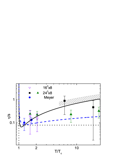
Figure 2: (Color online) The ratio of the gluon shear viscosity to the entropy density as a function of reduced temperature. Solid and dashed lines are computed with the averaged relaxation time obeying Eq. (77) and Eq. (76), respectively, with $2c=a_{2}=g^{2}(T_{c})$. The horizontal dotted line is the AdS/CFT bound $\eta/s=1/4\pi$  KSS03 . The lattice gauge ${\rm SU}(3)$ data with $16^{3}\times 8$ and $24^{3}\times 8$ lattice are from Ref. SN07 (triangles and squares) and Ma07 (filled circles). The shaded band corresponds to the perturbative result of Ref. AMY . The vertical dotted line shows the transition temperature.

The temperature dependence of the $\eta/s$ and $\zeta/s$ ratios is presented in Figs. 2 and 3, respectively. The lattice data SN07 were obtained using the lattice entropy from the old paper BEG95 . We corrected these data for $T/T_{c}>2$ in accordance with the new lattice QCD result Pa09 , which resulted in an increase of the lattice points in Figs. 2 and 3 by about 20% compared to the original paper SN07 . As we have noted, all three ansatze result in the same values of the shear viscosity. The dashed and solid curves in Fig. 2, corresponding to the two parametrizations (76) and (77) of the averaged relaxation time $\bar{\tau}$, have similar trends but different absolute values. With selected parameters $c$ and $a_{2}$ in (76) and (77) the curves exhibit discontinuity at the critical temperature $T_{c}$. Using (77) we can accurately describe the perturbative tail at very high temperatures.

In Fig. 3, calculations using different expressions for the bulk viscosity are compared with the lattice result. One should note that although the presented lattice data are not very conclusive due to large error bars, nevertheless, one may make some conclusions.

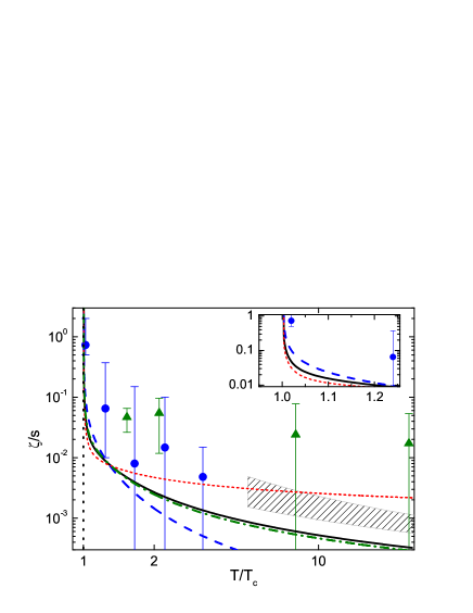
Figure 3: (Color online) The ratio of the gluon bulk viscosity to the entropy density as a function of temperature. The solid and long-dashed curves are calculated following Eq. (43) (ansatz I) with relaxation time from (77) and (76), respectively. The short-dashed curve is the ansatz II result [Eq. (59)] for the relaxation time from Eq. (77). The dash-dotted line corresponds to the ansatz III calculations [Eq. (70)] with parametrization (77). Lattice points are taken from SN07 (triangles) and Me08 (filled circles). The shaded band corresponds to the perturbative result from Ref. Arnold1 . The vertical dotted line shows the transition temperature.

The $\zeta/s$ ratios calculated with the relaxation time (77) within ansatze I, II, and III are presented by the solid, short-dashed, and dash-dotted curves, respectively. The results for ansatz I [Eq. (43), solid curve] and ansatz III [Eq.(70), dash-dotted curve] are very close to each other, in agreement with (74), whereas the ansatz II result [(59), short-dashed curve] differs from them significantly and overestimates lattice data in the perturbative regime. The result (59) of ansatz II with the relaxation time (76) (see Fig. 4 of KTVglue1 ) proves to be close to those presented by the solid and dash-dotted curves. On the other hand, the result (43) (long-dashed curve, ansatz I) with the relaxation time (76) perhaps underestimates the lattice data, whereas in the nonperturbative regime (at $T\sim T_{c}$) the long-dashed curve using the relaxation time (76) is closer to the data points than the solid curve using the relaxation time (77).

V Conclusions

We obtained expressions for the gluon shear and bulk viscosities within the relaxation time approximation by making use of an averaged value for the relaxation time $\tau=\widetilde{\tau}=\bar{\tau}$. Under this assumption, the expressions for the shear viscosity within ansatz I [Eq. (35)], ansatz II, and ansatz III [Eq. (58] coincide, which indicates robustness of the shear viscosity to the ansatz reductions performed.

In contrast, the expressions for the bulk viscosity, (43), (59), and (70), obtained within ansatze I, II, and III, respectively, significantly differ. Our numerical analysis demonstrates that the results (43) and (70) for gluons those mass increases with temperature, which use the Landau-Lifshitz condition (26), are close to each other in the whole range of temperatures whereas the result (59) using a modified Landau-Lifshitz condition (27) deviates from them significantly. One should stress that the result (59) is also recovered if in making variations one does not vary quantities which depend on the distribution function only implicitly, such as $E$ within ansatz I. The later approximation is fully justified only for nonrelativistic systems.

Among the results for the bulk viscosity, Eq. (43) seems to us most theoretically established. Nevertheless, all evaluations of the shear and bulk viscosities obtained in the framework of the relaxation time approximation can be considered only as rough estimations. In order to perform more established calculations, one should go beyond the scope of the relaxation time approximation. However, such calculations are much more involved than estimations presented in the given work and have not yet been carried out for systems with strong interactions.

Viscosity coefficients in a weakly coupled scalar field theory at arbitrary temperature can be evaluated directly from first principles without reference to the relaxation time approximation. This has been done by considering the expansion of the Kubo formulas in terms of ladder diagrams in the imaginary time formalism. In a theory with cubic and quartic interactions, the infinite class of diagrams which contribute to the leading weak-coupling behavior are identified and summed. The resulting expression is reduced to a single linear integral equation, which is shown to be identical to the corresponding result obtained from a linearized Boltzmann equation similar to those which arise when the Boltzmann equation is treated in the relaxation time approximation, as was first noted in Refs. Je94 ; VB02 . Unfortunately, a similar analysis for more general cases is unavailable.

Acknowledgements

We are grateful to Pavel Buividovich and Eugeny Kolomeitsev for useful discussions. This work was supported by RFBR Grant No. 11-02-01538-a and a grant from the European network I3-HP2 Toric.

References

- (1) P. Romatschke, Int. J. Mod. Phys. E 19, 1 (2010).
- (2) K. Aamodt et al., e-Print: arXiv:1011.3914 [nucl-ex].
- (3) G. Boyd, J. Engels, F. Karsch, E. Laermann, C. Legeland, M. Lütgemeier, and B. Petersson, Phys. Rev. Lett. 75, 4169 (1995); Nucl. Phys. B 469, 419 (1996).
- (4) M. Panero, Phys. Rev. Lett. 103, 232001 (2009).
- (5) S. Sakai and A. Nakamura, PoS LAT2007, 221 (2007).
- (6) H. B. Meyer, Phys. Rev. D 76, 101701 (2007).
- (7) H. B. Meyer, Phys. Rev. Lett. 100, 162001 (2008).
- (8) A. Peshier, B. Kämpfer, O. P. Pavlenko, and G. Soff, Phys. Rev. D 54, 2399 (1996).
- (9) A. Peshier and W. Cassing, Phys. Rev. Lett. 94, 172301 (2005).
- (10) Yu. B. Ivanov, V. V. Skokov, and V. D. Toneev, Phys. Rev. D 71, 014005 (2005).
- (11) A. S. Khvorostukhin, V. D. Toneev, and D. N. Voskresensky, arXiv:0912.2191, Phys. Atom. Nucl. 74, 650 (2011).
- (12) A. S. Khvorostukhin, V. D. Toneev, and D. N. Voskresensky, Nucl. Phys. A 845, 106 (2010).
- (13) A. Nakamura and S. Sakai, Phys. Rev. Lett. 94, 072305 (2005).
- (14) J.-W. Chen, J. Deng, H. Dong, and Q. Wang, Phys. Rev. D 83, 034031 (2011).
- (15) M. Bluhm, B. Kämpfer, and K. Redlich, Nucl. Phys. A 830, 737c (2009).
- (16) A. S. Khvorostukhin, V. D. Toneev, and D. N. Voskresensky, Phys. Rev. C 83, 035204 (2011).
- (17) M. Bluhm, B. Kämpfer, and K. Redlich, arXiv: 1011.5634 [hep-ph]; arXiv: 1012.0488 [hep-ph].
- (18) S. K. Das and J. Alam, Phys. Rev. D 83, 114011 (2011).
- (19) M. I. Gorenstein and S. N. Yang, Phys. Rev. D 52, 5206 (1995).
- (20) O. Kaczmarek, PoS CPOD07, 043 (2007).
- (21) A. A. Abrikosov and I. M. Khalatnikov, Rept. Progr. Phys. 22, 329 (1959).
- (22) Yu. B. Ivanov, J. Knoll, and D. N. Voskresensky, Nucl. Phys. A 672, 313 (2000); D. N. Voskresensky, Nucl. Phys. A 849, 120 (2011).
- (23) P. Chakraborty and J. I. Kapusta, Phys. Rev. C 83, 014906 (2011).
- (24) S. Gavin, Nucl. Phys. A 435, 826 (1985).
- (25) P. Kovtun, T. D. Son and O. A. Starinets, JHEP 0310, 064 (2003); Phys. Rev. Lett. 94, 111601 (2005).
- (26) P. Arnold, G. D. Moore and L. G. Yaffe, JHEP 0305, 051 (2003).
- (27) P. Arnold, Ç. Doǧan, and G. D. Moore, Phys. Rev. D 74, 085021 (2006).
- (28) S. Jeon, Phys. Rev. D 52, 3591 (1995).
- (29) M. A. Valle Basagoiti, Phys. Rev. D 66, 045005 (2002).