Multilevel Monte Carlo method for jump-diffusion SDEs

Abstract

We investigate the extension of the multilevel Monte Carlo path simulation method to jump-diffusion SDEs. We consider models with finite rate activity , using a jump-adapted discretisation in which the jump times are computed and added to the standard uniform discretisation times. The key component in multilevel analysis is the calculation of an expected payoff difference between a coarse path simulation and a fine path simulation with twice as many timesteps. If the Poisson jump rate is constant, the jump times are the same on both paths and the multilevel extension is relatively straightforward, but the implementation is more complex in the case of state-dependent jump rates for which the jump times naturally differ.

1 Introduction

In the Black-Scholes Model, the price of an option is given by the expected value of a payoff depending upon the solution of a stochastic differential equation(SDE) satisfied by the stock price. The model assumes that the behavior of the stock price is depicted by a SDE driven by Brownian motion,

$${\rm d}S(t)=a(S,t)\,{\rm d}t+b(S,t)\,{\rm d}W(t),\quad 0\leq t\leq T,$$ (1)

with given initial data $S_{0}$.

Although this model is widely used, the fact that asset returns are not log-normal has motivated people to suggest models which better capture the characteristics of the stock price dynamics. Merton[Mer76] proposed a jump-diffusion process for the stock price. To be specific, the stock price follows a jump-diffusion SDE:

$${\rm d}S(t)=a(S(t-),t){\rm d}t+b(S(t-),t){\rm d}W(t)+c(S(t-),t){\rm d}J(t),\quad 0\leq t\leq T,$$ (2)

where the jump term $J(t)$ is a compound Poisson process $\sum_{i=1}^{N(t)}(Y_{i}-1)$, the jump magnitude  $Y_{i}$ has a prescribed distribution, and $N(t)$ is a Poisson process with intensity $\lambda$, independent of the Brownian motion. Due to the existence of jumps, the process is a càdlàg process, i.e. having right continuity with left limits. We note that $S(t-)$ denotes the left limit of the process while $S(t)=\lim_{s\rightarrow t+}S(t)$. In [Mer76], Merton also assumed that $\log Y_{i}$ has a normal distribution with mean $a$ and variance $b$, namely $\log Y_{i}\sim N(a,b)$.

There are several ways to generalize Merton model from different aspects. A possible way is to consider the case where the frequency of jump is infinite, where general Lévy processes can be used. Another direction (for example in [GM03]) is to introduce dependency between parameters, leaving the expected number of jumps finite within finite horizon. As a particular numerical examples, we consider the case where instantaneous jump rate relies on the stock price, namely $\lambda(t)=\lambda(S_{t},t)$.

In pursuit of risk-neutral pricing of options, we are interested in the expected value of a function of the terminal state, $f(S(T))$. In the simple case of a European option, the expectation can be directly simulated, while in the case of Asian, lookback and barrier options the valuation depends on the entire path $S(t),0\leq t\leq T$. The expected value can be estimated by a simple Monte Carlo method with a proper numerical discretisation scheme. However, to achieve a root-mean-square (RMS) error of $O({\epsilon})$ using an Euler-Maruyama discretisation would require $O({\epsilon}^{-2})$ independent paths, each with $O({\epsilon}^{-1})$ timesteps, leading to a computational complexity of $O({\epsilon}^{-3})$. This is quite time consuming compared to the case of path-independent options.

Giles [Gil07] [Gil08b] has recently introduced a multilevel Monte Carlo path simulation method for the option pricing calculation. This improves the computational efficiency of Monte Carlo path simulation by combining results using different numbers of timesteps. This can be viewed as a generalisation of the two-level method of Kebaier [Keb05] and is also similar in approach to Heinrich’s multilevel method for parametric integration [Hei01]. The first paper [Gil08b] proposed the multilevel Monte Carlo approach and proved that it can lower the computational complexity of path-dependent Monte Carlo evaluations to $O({\epsilon}^{-2}(\log{\epsilon})^{2})$, verified by numerical results using the simple Euler-Maruyama discretisation. The second paper [Gil07] demonstrated that the computational cost can be further reduced to $O({\epsilon}^{-2})$ by using the Milstein discretisation. This has been extended by Dereich and Heidenreich [DH11, Der11] to approximation methods for both finite and infinite activity Lévy-driven SDEs with globally Lipschitz payoffs. The work in this paper differs in considering simpler finite activity jump-diffusion models, but more challenging non-Lipschitz payoffs, and also uses a more accurate Milstein discretisation to achieve an improved order of convergence for the multilevel correction variance which will be defined later.

In this paper we applies the multilevel approach to the Monte Carlo simulation of path-dependent option pricing under jump-diffusion processes. We first consider the case where the jump rate is constant then take into account the state-dependent rate case. In both cases, in order to calculate coarse-path samples from fine-path sample using brownian interpolation , we adopt a jump-adapted Milstein discretisation scheme proposed by [Pla82], which explicitly simulates the times when jumps occur. Furthermore, we construct multilevel estimators for corresponding path-dependent payoffs coping with challenges caused by jumps. Through constructing payoff estimators by Brownian bridge technique, high order multilevel correction term variance convergence rate is achieved. In the state-dependent rate case, we use two approaches, which are called cumulative intensity method and thinning method to tackle the unsynchronization of jump times in the fine and coarse grids. Numerical results show similar improvement in computational efficiency compared with previous achievement [Gil07] for diffusion processes. Generally, using the jump-adapted Milstein scheme with the multilevel approach, we can reduce the computation cost to $O({\epsilon}^{-2})$ in terms of RMS error ${\epsilon}$.

In the following parts of the paper, we first review the Multilevel Monte Carlo method for diffusion processes. The next section describes the jump-adapted discretisation of jump-diffusion processes and its advantages for facilitating the multilevel approach. Then we discuss the path simulation and estimator construction for the jump-adapted discretisation with the multilevel approach and present numerical results of Asian, lookback, barrier and digital options. The next part establishes two methods to deal with state-dependent intensity. The final section draws conclusions and indicates directions of future research.

2 Multilevel Monte Carlo method

Suppose we perform Monte Carlo path simulations with fixed grid timesteps $h_{\ell}=2^{-\ell}\,T$, $l=0,1,\ldots,L$. For a given Brownian path $W(t)$, let $P$ denote the payoff, and let ${\widehat{P}}_{\ell}$ denote its approximation by a numerical scheme with timestep $h_{\ell}$. As a result of the linearity of the expectation operator,

$${\mathbb{E}}[{\widehat{P}}_{L}]={\mathbb{E}}[{\widehat{P}}_{0}]+\sum_{\ell=1}^{L}{\mathbb{E}}[{\widehat{P}}_{\ell}\!-\!{\widehat{P}}_{\ell-1}].$$ (3)

Let ${\widehat{Y}}_{0}$ denote an estimator for ${\mathbb{E}}[{\widehat{P}}_{0}]$ using $N_{0}$ paths. Suppose for different $l>0$, we use $N_{\ell}$ independent paths to estimate ${\mathbb{E}}[{\widehat{P}}_{\ell}\!-\!{\widehat{P}}_{\ell-1}]$.

$${\widehat{Y}}_{\ell}=N_{\ell}^{-1}\sum_{i=1}^{N_{\ell}}\left({\widehat{P}}_{\ell}^{(i)}\!-\!{\widehat{P}}_{\ell-1}^{(i)}\right).$$ (4)

The Multilevel method facilitates the fact that ${\mathbb{V}}[{\widehat{P}}_{\ell}\!-\!{\widehat{P}}_{\ell-1}]$ decreases with $l$ to adaptively choose $N_{\ell}$ and hence reduce the computational cost.

The cost reduction effect is summarized in the following theorem:

Theorem 2.0.1.

Let $P$ denote a functional of the solution of stochastic differential equation (1) for a given Brownian path $W(t)$, and let ${\widehat{P}}_{\ell}$ denote the corresponding approximation using a numerical discretisation with timestep $h_{\ell}=2^{-l}\,T$.

If there exist independent estimators ${\widehat{Y}}_{\ell}$ based on $N_{\ell}$ Monte Carlo samples, and positive constants $\alpha\!\geq\!{\ \textstyle\frac{1}{2}},\beta,c_{1},c_{2},c_{3}$ such that

• $\displaystyle\left|{\mathbb{E}}[{\widehat{P}}_{\ell}-P]\right|\leq c_{1}\,h_{\ell}^{\alpha}$

• $\displaystyle{\mathbb{E}}[{\widehat{Y}}_{\ell}]=\left\{\begin{array}[]{ll}{\mathbb{E}}[{\widehat{P}}_{0}],&l=0\\[7.22743pt] {\mathbb{E}}[{\widehat{P}}_{\ell}-{\widehat{P}}_{\ell-1}],&l>0\end{array}\right.$

• $\displaystyle{\mathbb{V}}[{\widehat{Y}}_{\ell}]\leq c_{2}\,N_{\ell}^{-1}h_{\ell}^{\beta}$

• $C_{\ell}$, the computational complexity of ${\widehat{Y}}_{\ell}$, is bounded by

  $$C_{\ell}\leq c_{3}\,N_{\ell}\,h_{\ell}^{-1},$$

then there exists a positive constant $c_{4}$ such that for any ${\epsilon}\!<\!e^{-1}$ there are values $L$ and $N_{\ell}$ for which the multilevel estimator

$${\widehat{Y}}=\sum_{\ell=0}^{L}{\widehat{Y}}_{\ell},$$

has a mean-square-error with bound

$$MSE\equiv{\mathbb{E}}\left[\left({\widehat{Y}}-{\mathbb{E}}[P]\right)^{2}\right]<{\epsilon}^{2}$$

with a computational complexity $C$ with bound

$$C\leq\left\{\begin{array}[]{ll}c_{4}\,{\epsilon}^{-2},&\beta>1,\\[7.22743pt] c_{4}\,{\epsilon}^{-2}(\log{\epsilon})^{2},&\beta=1,\\[7.22743pt] c_{4}\,{\epsilon}^{-2-(1-\beta)/\alpha},&0<\beta<1.\end{array}\right.$$

Proof.

See [Gil08b]. ∎

In the case of the jump-adapted discretisation, $h_{\ell}$ should be taken to be the uniform timestep at level $l$, to which the jump times are added to form the set of discretisation times. We have to define the computational complexity as the expected computational cost since different paths may have different numbers of jumps. However, the expected number of jumps is finite and therefore the cost bound in assumption iv) will still remain valid for an appropriate choice of the constant $c_{3}$.

According to the theorem, the larger the variance convergence rate $\beta$ , the greater the reduction is the computation cost by the multilevel algorithm. In the case of a Lipschitz continuous European payoff, using the Milstein discretisation immediately leads to the result that $V_{\ell}=O(h_{\ell}^{2})$, corresponding to $\beta\!=\!2$. Thus the main task to improve the performance of the multilevel method is to use using schemes with high order strong convergence rate and constructing appropriate estimators so that $\beta>1$ could be achieved. For the jump-diffusion process, the objective is to obtain $\beta>1$ through adopting a high order scheme.

3 A Jump-adapted Milstein discretisation

To simulate jump-diffusion processes, it is possible to use fixed time grid schemes as for geometric Brownian motion. The Euler-Maruyama scheme for jump-diffusion processes has $O(\sqrt{h})$ strong convergence ([Pla10]). However, it would be more difficult to pursue higher order strong convergence. To achieve a higher order strong convergence for jump-diffusion processes, the Itô-Taylor expansion will involve some double integrals of white noise and the Poisson random measure [BLP05], which increases the complexity of the simulation.

Another problem which might be encountered for fixed-time grid schemes is the construction of estimators for the payoff function of path-dependent options. Adoption of the previous Brownian bridge interpolation is difficult since the minimum or other functional of paths is difficult to calculate since the joint density of diffusion and jump is much more complex than pure diffusion one.

In order to avoid simulating double stochastic integrals as well as to identify the time at which the jump occurs, we use the so-called jump-adapted approximation proposed by Platen in [Pla82]. This jump-adapted scheme would improve the computational tractability compared to other fixed time grid discretisation schemes with the same weak/strong convergence order.

Suppose that we have simulated the jump time grid $\mathbb{J}=\{\tau_{1},\tau_{2},\ldots,\tau_{m}\}$, which includes times at which jumps occur in the $[0,T]$. On the other hand, consider a fixed time grid constituted by $N$ timesteps, $t_{i}^{\prime}=i\times\frac{T}{N},~{}i=1,\ldots,N,$ which is used in discretisation schemes of Brownian SDEs. Now consider a superposition of them as a new grid $\mathbb{T}=\{0=t_{0}<t_{1}<t_{2}<\ldots<t_{M}=T\}$. As a result, the length of timestep of the new grid will be no greater than $h=\frac{T}{N}$.

Within every timestep of the new grid, the diffusion part is separated from the effect of the possible jump, because the jump only occurs at the grid point. Thus we can approximate the path with established schemes for diffusion processes, and deal with corresponding adjustment if there is a jump at the right end of interval. This procedure is called the jump-adapted scheme.

The algorithm of simulation via the jump-adapted scheme could be described as the following steps:

1. Set $i=1,~{}j=1$, $t^{\prime}=t^{\prime}_{0}$;

2. Generate jump time $\tau_{i}$ in terms of its distribution;

3. While $(\tau_{i}<t^{\prime}_{j})$ do

   (1). Simulate the process within $[t^{\prime},\tau_{i})$, in which the process is driven purely by Brownian motion, then simulate the jump at $\tau_{i}$;

   (2). Set the timestep $h_{i}=\tau_{i}-t^{\prime}$, $t^{\prime}=\tau_{i}$;

   (3). $i=i+1$, and generate next jump time $\tau_{i}$ in terms of its distribution;

4. Simulate the process within $[t^{\prime},t^{\prime}_{j}]$;

5. Set the timestep $h_{i}=\tau_{i}-t^{\prime}$, $j=j+1$, $t^{\prime}=t^{\prime}_{j}$ and goto 3.

Now we introduce a jump-adapted Milstein scheme for a scalar jump-diffusion SDE

$${\widehat{S}}_{n+1}^{-} = {\widehat{S}}_{n}+a_{n}\,h_{n}+b_{n}\,\Delta W_{n}+{\textstyle\frac{1}{2}}\,\frac{\partial b_{n}}{\partial S}\,b_{n}\,(\Delta W_{n}^{2}-h_{n}),$$

$${\widehat{S}}_{n+1} = \left\{\begin{array}[]{lll}&{\widehat{S}}_{n+1}^{-}+c({\widehat{S}}_{n+1}^{-},t_{n+1})(Y_{i}-1),&\text{ when}~{}t_{n+1}=\tau_{i};\\ &{\widehat{S}}_{n+1}^{-},&\text{ otherwise}.\end{array}\right.$$

Where the subscript $n$ is used to denotes the timestep index, ${\widehat{S}}_{n}^{-}={\widehat{S}}(t_{n}-)$ is the left limit of the approximated solution, and $Y_{i}$ is the jump magnitude at $\tau_{i}$.

In sum, jump-adapted schemes explicitly compute jump times, which are relatively rare in the entire time span. Thus, compared to fixed time schemes, they save the computation cost for generating Poisson random numbers when the timestep tends to zero. Furthermore, as we will see later, in terms of path simulation, jump-adapted discretisations have a very crucial property that keeps the multilevel approach valid: within each timestep we can neglect the jump term and only take the Brownian component into consideration. As a matter of fact, the scheme can conveniently adopt the Brownian bridge technique used for estimator construction in the previous paper [Gil07] so that improved convergence could be obtained as well.

4 Multilevel approach in the presence of jump

In all of the cases to be presented, we simulate the paths using the jump-adapted Milstein scheme proposed above.

In the case of a jump-diffusion process, since theorem of computation complexity in the case of diffusion processes requires the weak convergence and ML estimator convergence of discretisation schemes, we have to justify them accordingly for different construction of estimators. These numerical analysis is being done in a working paper in preparation [XG11].

Apart from theoretical issues, there arise two challenges in the implementation. The first problem is that the path simulation on coarse levels needs to be revised in the presence of varying timesteps of the jump-adapted time grid. Another is how to devise suitable estimators for various payoffs in coping with a jump-adapted time grid. The third concern is whether optimal samples on each level used by previous algorithm in [Gil08b] should be modified. Due to presence of jump, the computational cost is

$$Cost=\sum_{\ell=0}^{L}\sum_{i=1}^{N_{\ell}}(N_{T}^{(i)}+2^{\ell}),$$

where $N_{T}^{(i)}$ is the number of jumps in each scenario. However, the expected number of jumps is finite and therefore the cost bound in assumption iv) will still remain valid for an appropriate choice of the constant $c_{3}$ therefore using previous algorithm should work well. In implementation numerical results indicates that this is appropierate for small $\lambda.$

4.1 Path simulation of multilevel approach in the jump-adapted time grid

When the multilevel approach is applied to the simulation with a fixed time discretisation of a jump-diffusion process, the algorithm maintains the orinigal framework straightforward. While for jump-adapted schemes, construction of coarse path simulation needed for the estimators (4) of the payoff differs from previous case.

In the case of fixed time grid for geometric Brownian motion, every path sample used for calculating ${\widehat{P}}_{\ell}^{(i)}\!-\!{\widehat{P}}_{\ell-1}^{(i)}$ comes from two discrete approximations of Brownian path, which are called the fine path and the coarse path. For every $l$, every timestep of coarse grid is completely the same as the corresponding two timesteps of the fine grid starting from the same endpoint. Since the brownian increment of the coarse timestep is equidistributed to the sum of two increments of corresponding fine ones, we can do the coarse path simulation without generating extra random normal number.

While in the case of jump-adapted time grid, due to the presence of jump time, the construction of a path sample in the coarse grid using the brownian increments generated in the fine grid needs to be clarified. In this case, the path sample is discontinuous in its jump time. To avoid such discontinuity, notice that within each timestep of jump-adapted time grid, the path is purely driven by Brownian component and therefore reserves continuity. For the coarse grid and the fine grid in the same level, call the finer grid points midpoints for short. For a particular midpoint, the timestep, which is formed by the last jump time before this midpoint and the first jump time after it is called midpoint timestep. In this timestep, Brownian increment of the coarse path sample can be obtained by the summation of Brownian increments of corresponding two timestep in fine grid. In remaining timesteps of coarse grid, construction of the coarse path sample uses the same Brownian increment as the one in fine grid does. Hence we have defined the coarse path sample construction according to this midpoint construction, which can be seen clearly in figure 1.

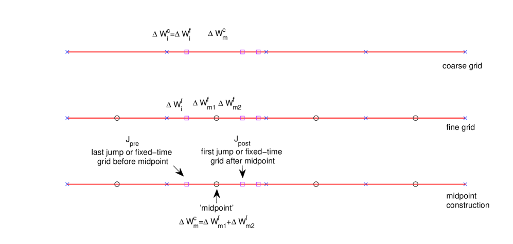
Figure 1: Midpoint construction

4.2 Estimator construction

For the estimator construction, there comes concern whether extra bias is introduced for estimator in the jump-diffusion process. To secure the correctness of the identity3, we must avoid introducing any undesired bias, hence it is required that

$${\mathbb{E}}[{\widehat{P}}_{\ell}^{f}]={\mathbb{E}}[{\widehat{P}}_{\ell}^{c}].$$ (6)

This means that the definitions of ${\widehat{P}}_{\ell}$ when estimating $E[{\widehat{P}}_{\ell}\!-\!{\widehat{P}}_{\ell-1}]$ and $E[{\widehat{P}}_{\ell+1}\!-\!{\widehat{P}}_{\ell}]$ must have the same expectation.

In the case of path-dependent payoffs in geometric Brownian motion, we approximate the payoff function by Brownian bridge interpolation technique using path values on the fine and the coarse grid. This technique is also available in jump case to reduce the variance of the estimator, where the coarse-path estimator will involve the information from generations of fine-path sample in the two corresponding timesteps. One thing to notice in jump-adapted schemes is that we can utilise this construction only for the timesteps including midpoint. For other timesteps of coarse grid, the construction of coarse-grid estimators will be the same as the fine-grid one. Estimators will be discussed in the following respectively corresponding to their payoffs.

In the following we will show the numerical results of several options. All of them are done for Merton model in which the jump-diffusion SDE under risk-neutral measure is

$$\dfrac{{\rm d}S(t)}{S(t-)}=(r-\lambda m)\,{\rm d}t+{\sigma}\,{\rm d}W(t)+{\rm d}J(t),\quad 0\leq t\leq T.$$

where $\lambda$ is the jump intensity and jump magnitude satisfies $\log Y_{i}\sim N(a,b)$, $r$ is the risk-free rate, ${\sigma}$ is the volatility of stock price and $m={\mathbb{E}}[Y_{i}]-1$ is the compensator to ensure the discounted stock price is a martingale. All of the simulations in this section use the parameter values $S_{0}\!=\!100$, $K\!=\!100$, $T\!=\!1$, $r\!=\!0.05$, ${\sigma}\!=\!0.2$, $a\!=\!0.1$, $b\!=\!0.2$, $\lambda\!=\!1$. We thank Giles providing the code for [Gil08a], based on which we can produce the current code to generate numerical results and figures.

4.3 Vanilla call option

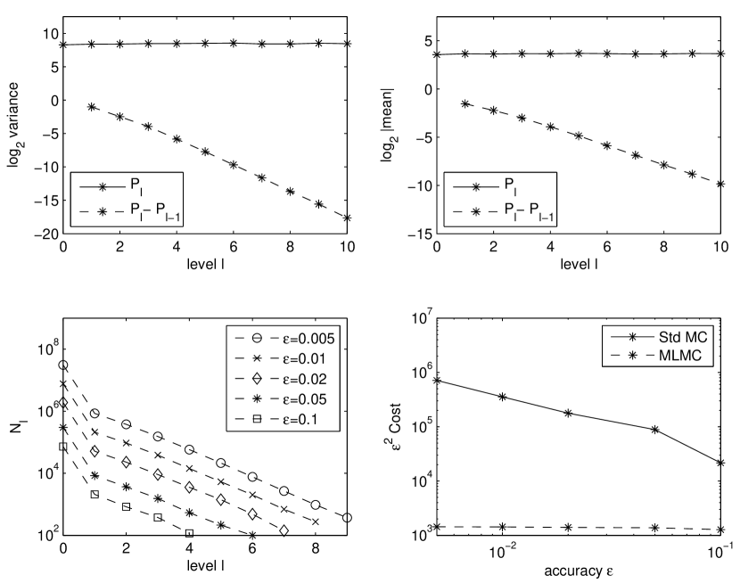
Figure 2: Vanilla option

For the vanilla option with the payoff $\exp(-rT)\max(S(T)-K,0)$, Figure 2 shows the numerical results.

The top left plot shows the behaviour of the variance of both ${\widehat{P}}_{\ell}$ and the multilevel correction ${\widehat{P}}_{\ell}\!-\!{\widehat{P}}_{\ell-1}$, estimated using $10^{5}$ samples so that the Monte Carlo sampling error is negligible. The slope of the MLMC line indicates that $V_{\ell}\!\equiv\!{\mathbb{V}}[{\widehat{P}}_{\ell}\!-\!{\widehat{P}}_{\ell-1}]\!=\!O(h_{\ell}^{2})$, corresponding to $\beta=2$ in condition $iii)$ of Theorem 2.0.1. The top right plot shows that ${\mathbb{E}}[{\widehat{P}}_{\ell}\!-\!{\widehat{P}}_{\ell-1}]$ is approximately $O(h_{\ell})$, corresponding to $\alpha=1$ in condition $i)$. Noting that the payoff is Lipschitz, both of these are consistent with the first order strong convergence proved in [Pla10].

The bottom two plots correspond to five different multilevel calculations with different user-specified accuracies to be achieved. These use the numerical algorithm given in [Gil08b] to determine the number of grid levels, and the optimal number of samples on each level, which are required to achieve the desired accuracy. We use the computational cost $\sum_{\ell=0}^{\ell}\sum_{i=1}^{N_{\ell}}(N_{T}^{(i)}+2^{\ell})$ to take account into the effect of jump. The left plot shows that in each case many more samples are used on level 0 than on any other level, with very few samples used on the finest level of resolution. The right plot shows that the the multilevel cost is approximately proportional to ${\epsilon}^{-2}$, which agrees with the computational complexity bound in Theorem 2.0.1 for the $\beta\!>\!1$ case.

4.4 Asian option

The payoff of the Asian option we consider is

$$P=\exp(-rT)\ \max\left(0,\overline{S}\!-\!K\right),$$

where

$$\overline{S}=T^{-1}\int_{0}^{T}S(t)\ {\rm d}t.$$

$n_{T}\!=\!T/h$ is the number of timesteps. [Gil07] shows that accuracy can be achieved by approximating the behaviour of a process within a timestep as an It̂o process with constant drift and volatility, conditional on the computed endpoint values ${\widehat{S}}_{n}$. Taking $b_{n}$ to be the constant volatility within the interval $[t_{n},t_{n+1}]$, in other words, we define brownian interpolation in the coarse grid at $t$ as

$${\widehat{S}}(t)={\widehat{S}}_{n}+\mu({\widehat{S}}_{n+1}^{-}-{\widehat{S}}_{n})+b_{n}[W_{t}-W_{n}-\mu(W_{n+1}-W_{n})],$$ (7)

where $\mu=(t-t_{n})/h,~{}h=t_{n+1}-t_{n}$.

This implies

$$\int_{t_{n}}^{t_{n+1}}{\widehat{S}}(t)\ {\rm d}t={\ \textstyle\frac{1}{2}}h(S(t_{n})+S(t_{n+1}-))+b_{n}\Delta I_{n},$$

where $\Delta I_{n}$ is

$$\Delta I_{n}:=\int_{t_{n}}^{t_{n+1}}(W(t)-W(t_{n}))\ {\rm d}t\ -\ {\ \textstyle\frac{1}{2}}\,h\Delta W,$$

satisfying $\Delta I_{n}\sim N(0,h^{3}/12)$ , and is independent of $\Delta W$. Let $b_{n}=b({\widehat{S}}_{n},t_{n})$, the fine-path approximated payoff would be

$$\overline{S}^{f}=T^{-1}\sum_{n=0}^{n_{T}-1}\left({\ \textstyle\frac{1}{2}}\,h\,({\widehat{S}}_{n}\!+\!{\widehat{S}}_{n+1}^{-})+b_{n}\Delta I_{n}^{f}\right).$$

In a jump-adapted grid, the coarse-path approximation is the same in most timesteps except in the midpoint timestep $\Delta I_{n}^{c}$ is derived from the fine-path values, namely

Figure 3: Asian option

$$\int_{t_{n}}^{t_{n+2}}(W(t)-W(t_{n}))\ {\rm d}t\ -\ \textstyle\frac{1}{2}(t_{n+2}-t_{n})(W(t_{n+2})-W(t_{n}))$$

$$= \int_{t_{n}}^{t_{n+1}}(W(t)-W(t_{n}))\ {\rm d}t\ -\ {\ \textstyle\frac{1}{2}}\,(t_{n+1}-t_{n})\left(W(t_{n+1})-W(t_{n})\right)$$

$$+ \int_{t_{n}+h}^{t_{n+2}}(W(t)-W(t_{n+1}))\ {\rm d}t\ -\ {\ \textstyle\frac{1}{2}}\,(t_{n+2}-t_{n+1})\left(W(t_{n+2})-W(t_{n+1})\right)$$

$$+ {\ \textstyle\frac{1}{2}}\,(t_{n+2}-t_{n+1})\left(W(t_{n+1})-W(t_{n})\right)-{\ \textstyle\frac{1}{2}}\,(t_{n+1}-t_{n})\left(W(t_{n+2})-W(t_{n+1})\right),$$

and thus

$$\Delta I^{c}=\Delta I^{f1}_{n}+\Delta I^{f2}_{n}+{\ \textstyle\frac{1}{2}}\,(t_{n+2}-t_{n})(\mu\Delta W^{f1}-(1-\mu)\Delta W^{f2}),$$

where $\mu_{n}=(t_{n+2}-t_{n+1})/(t_{n+2}-t_{n})$, $\Delta I^{c}$ is the value for the coarse timestep in midpoint timestep; $\Delta I^{f1}$ and $\Delta W^{f1}$ are the values for fine timestep in the first fine-path timestep constituting the midpoint timestep; $\Delta I^{f2}$ and $\Delta W^{f2}$ are the values for the fine timestep in the latter one constituting the midpoint timestep.

Figure 3 shows the numerical results for parameters $S(0)\!=\!100$, $K\!=\!100$, $T\!=\!1$, $r\!=\!0.05$, ${\sigma}\!=\!0.2$, $a\!=\!0.1$, $b\!=\!0.2$, $\lambda\!=\!1$. All the results are similar to the pure diffusion case.

4.5 Lookback option

The payoff of the lookback option we consider is

$$P=\exp(-rT)\left(S(T)-\min_{0\leq t\leq T}S(t)\right).$$

Previous work [Gil07] achieved a second order convergence rate for the multilevel correction variance using the Milstein discretisation and an estimator constructed by approximating the behaviour within a timestep as an Itô process with constant drift and volatility, conditional on the endpoint values ${\widehat{S}}_{n}$ and ${\widehat{S}}_{n+1}$. Brownian Bridge results (see section 6.4 in [Gla04]) give the minimum value within the timestep $[t_{n},t_{n+1}]$, conditional on the end values, as

$${\widehat{S}}_{n,min}={\ \textstyle\frac{1}{2}}\left({\widehat{S}}_{n}+{\widehat{S}}_{n+1}-\sqrt{\left({\widehat{S}}_{n+1}\!-\!{\widehat{S}}_{n}\right)^{2}-2\,b_{n}^{2}\,h\log U_{n}}\ \right),$$ (8)

where $b_{n}$ is the constant volatility and $U_{n}$ is a uniform random variable on $[0,1]$. The same treatment can be used for the jump-adapted discretisation in this paper, except that ${\widehat{S}}_{n+1}^{-}$ must be used in place of ${\widehat{S}}_{n+1}$ in (8).

Equation (8) is used for the fine path approximation, but a different treatment is used for the coarse path, as in [Gil07]. This involves a change to the original telescoping sum in (3) which now becomes

$${\mathbb{E}}[{\widehat{P}}^{f}_{L}]={\mathbb{E}}[{\widehat{P}}^{f}_{0}]+\sum_{\ell=1}^{L}{\mathbb{E}}[{\widehat{P}}^{f}_{\ell}\!-\!{\widehat{P}}^{c}_{\ell-1}],$$ (9)

where ${\widehat{P}}^{f}_{\ell}$ is the approximation on level $\ell$ when it is the finer of the two levels being considered, and ${\widehat{P}}^{c}_{\ell}$ is the approximation when it is the coarser of the two. This modified telescoping sum remains valid provided ${\mathbb{E}}[{\widehat{P}}^{f}_{\ell}]={\mathbb{E}}[{\widehat{P}}^{c}_{\ell}].$

Considering a particular timestep in the coarse path construction, we have two possible situations. If it does not contain one of the fine path discretisation times, and therefore corresponds exactly to one of the fine path timesteps, then it is treated in the same way as the fine path, using the same uniform random number $U_{n}$. This leads naturally to a very small difference in the respective minima for the two paths.

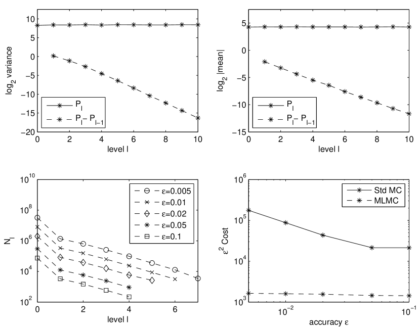
Figure 4: Lookback option

The more complicated case is the one in which the coarse timestep contains one of the fine path discretisation times $t^{\prime}$, and so corresponds to the union of two fine path timesteps. In this case, the value at time $t^{\prime}$ is given by the conditional Brownian interpolant

$${\widehat{S}}(t^{\prime})={\widehat{S}}_{n}+\mu\,({\widehat{S}}_{n+1}^{-}-{\widehat{S}}_{n})+b_{n}\left(W(t^{\prime})-W_{n}-\mu\,(W_{n+1}-W_{n})\right),$$ (10)

where $\mu=(t^{\prime}-t_{n})/(t_{n+1}-t_{n})$ and the value of $W(t^{\prime})$ comes from the fine path simulation. Given this value for ${\widehat{S}}(t^{\prime})$, the minimum values for $S(t)$ within the two intervals $[t_{n},t^{\prime}]$ and $[t^{\prime},t_{n+1}]$ can be simulated in the same way as before, using the same uniform random numbers as the two fine timesteps.

The equality ${\mathbb{E}}[{\widehat{P}}^{f}_{\ell}]={\mathbb{E}}[{\widehat{P}}^{c}_{\ell}]$ is respected in this treatment because $W(t^{\prime})$ comes from the correct distribution, conditional on $W_{n+1},W_{n}$, and therefore, conditional on the values of the Brownian path at the set of coarse discretisation points, the computed value for the coarse path minimum has exactly the same distribution as it would have if the fine path algorithm were applied.

Further discussion and analysis of this is given in [XG11], including a proof that the strong error between the analytic path and the conditional interpolation approximation is at worst $O(h\,\log h)$.

Figure 4 presents the numerical results. The results are very similar to those obtained by Giles for geometric Brownian motion [Gil07]. The top two plots indicate second order variance convergence rate and first order weak convergence, both of which are consistent with the $O(h\,\log h)$ strong convergence. The computational cost of the multilevel method is therefore proportional to ${\epsilon}^{-2}$, as shown in the bottom right plot.

4.6 Barrier option

We consider a down-and-out call barrier option for which the discounted payoff is

$$P=\exp(-rT)\,(S(T)\!-\!K)^{+}\,\mathbbm{1}_{\left\{M_{T}>B\right\}},$$

where $M_{T}=\min_{0\leq t\leq T}S(t).$ The jump-adapted Milstein discretisation with the Brownian interpolation gives the approximation

$${\widehat{P}}=\exp(-rT)\,({\widehat{S}}(T)\!-\!K)^{+}\,\mathbbm{1}_{\left\{\widehat{M}_{T}>B\right\}}$$

where $\widehat{M}_{T}=\min_{0\leq t\leq T}{\widehat{S}}(t)$. This could be simulated in exactly the same way as the lookback option, but in this case the payoff is a discontinuous function of the minimum $M_{T}$ and an $O(h)$ error in approximating $M_{T}$ would lead to an $O(h)$ variance for the multilevel correction.

Instead, following the approach of Cont & Tankov (see page 177 in [CT04]), it is better to use the expected value conditional on the values of the discrete Brownian increments and the jump times and magnitudes, all of which may be represented collectively as $\mathcal{F}$. This yields

$$\mathbb{E}\left[\exp(-rT)\ ({\widehat{S}}(T)\!-\!K)^{+}\mathbbm{1}_{\left\{\widehat{M}_{T}>B\right\}}\right]$$

$$= \mathbb{E}\left[\exp(-rT)\ ({\widehat{S}}(T)\!-\!K)^{+}\mathbb{E}\left[\mathbbm{1}_{\left\{\widehat{M}_{T}>B\right\}}\mid\mathcal{F}\right]\right]$$

$$= \mathbb{E}\left[\exp(-rT)\ ({\widehat{S}}(T)-K)^{+}\ \prod_{n=0}^{n_{T}-1}{\widehat{p}}_{n}\right]$$

where ${\widehat{p}}_{n}$ denotes the conditional probability that the path does not cross the barrier $B$ during the $n^{th}$ timestep:

$${\widehat{p}}_{n}=1-\exp\left(\frac{-2\,({\widehat{S}}_{n}\!-\!B)^{+}({\widehat{S}}_{n+1}^{-}\!-\!B)^{+}}{b_{n}^{2}\ (t_{n+1}-t_{n})}\right).$$ (11)

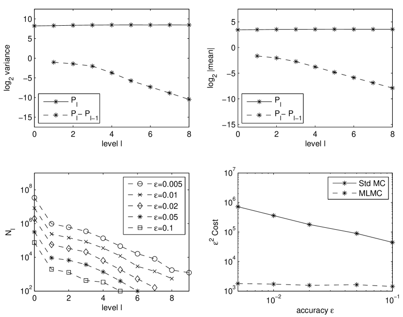
Figure 5: Barrier option

For fine-path value, we compute ${\widehat{p}}_{n}^{f}$ where $b_{n}$ is defined equal to $b({\widehat{S}}_{n},t_{n})$ within each timestep of the jump-adapted grid. Note that $S_{n+1}$ in (11) should be replaced by the value of left limit of the endpoint $S_{n+1}^{-}$, as in the lookback calculation.

For the coarse path calculation, we again deal separately with two cases. When the coarse timestep does not include a fine path time, then we again use (11). In the other case, when it includes a fine path time $t^{\prime}$ we evaluate the Brownian interpolant at $t^{\prime}$ and then use the conditional expectation to obtain

$${\widehat{p}}_{n} = \left\{1-\exp\left(\frac{-2\,({\widehat{S}}_{n}\!-\!B)^{+}({\widehat{S}}(t)\!-\!B)^{+}}{b_{n}^{2}\ (t^{\prime}-t_{n})}\right)\right\}$$ (12)

$$\times\ \left\{1-\exp\left(\frac{-2\,({\widehat{S}}(t^{\prime+}({\widehat{S}}_{n+1}^{-}\!-\!B)^{+}}{b_{n}^{2}\ (t_{n+1}-t^{\prime})}\right)\right\}.$$

Figure 5 shows the numerical results for $K\!=\!100$, $B\!=\!85$. The top left plot shows that the multilevel variance is $O(h_{\ell}^{\beta})$ for $\beta\approx 3/2$. This is similar to the behavior for a diffusion process [Gil07]. The bottom right plot shows that the computational cost of the multilevel method is again almost perfectly proportional to ${\epsilon}^{-2}$.

4.7 Digital option

The digital option considered here has the discounted payoff

$$P=\exp(-rT)\ \mathbbm{1}_{\{S(T)>K\}}.$$

In [Gil07], a multilevel variance convergence rate of $O(h_{\ell}^{3/2})$ is achieved by smoothing the payoff using conditional expectation given the brownian increments terminated one timestep before reaching the terminal time $T$. The estimator is the probability that ${\widehat{S}}_{n_{\ell}}>K$ under assumption of simple Brownian motion with constant drift $a_{n_{\ell}-1}$ and volatility $b_{n_{\ell}-1}$ within last timestep where $n_{\ell}$ denotes number of fine-path timesteps:

$${\mathbb{E}}[{\widehat{P}}_{\ell}-{\widehat{P}}_{\ell-1}] = {\mathbb{E}}[~{}{\mathbb{E}}[~{}f({\widehat{S}}_{n_{\ell}-1}^{f})-f({\widehat{S}}_{n_{\ell}-1}^{c})~{}|~{}\Delta W_{i},\ i=1,\ldots,n_{\ell}-1]~{}]$$

$$= {\mathbb{E}}[~{}\Phi\left(\frac{{\widehat{S}}_{n_{\ell}-1}^{f}\!+\!a_{n_{\ell}-1}^{f}h-K}{b_{n_{\ell}-1}^{f}\sqrt{h}}\right)-\Phi\left(\frac{{\widehat{S}}_{n_{\ell}-2}^{c}\!+\!2a_{n_{\ell}-2}^{c}h\!+\!b_{n_{\ell}-2}^{c}\Delta W_{n_{\ell}-1}-K}{b_{n_{\ell}-2}^{c}\sqrt{h}}\right)~{}],$$

where $\Phi$ is the cumulative density function of Normal variable, $h$ is fine-path fixed-time timestep.

In the jump-adapted time grid, the relation between last jump time and the last timestep before expiry leads to different expressions of above conditional expectation estimator. Let In fact, there would be three cases:

1. The last jump time $J$ happens before penultimate fixed-time timestep, i.e. $J<(N-2)\frac{T}{N}$, where $N$ is the number of timesteps in fixed-time fine grid;

2. The last jump time is within the last fixed-time timestep , i.e. $J>(N-1)\frac{T}{N}$;

3. The last jump time is within penultimate fixed-time timestep, i.e. $(N-1)\frac{T}{N}>J>(N-2)\frac{T}{N}$.

Correspondingly, different fine-path and coarse-path estimators are shown in the following.

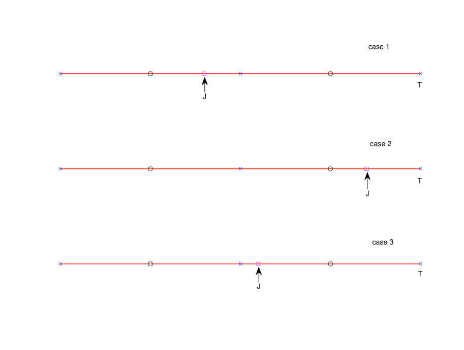
Figure 6: Construction of conditional expectation estimator for Digital option

1. In case 1, the fine-path grid and coarse-path grid is the same as the previous diffusion case, hence we do not need to change the estimator, which is the probability that ${\widehat{S}}_{n_{T}}>K$ under assumption of approximation the dynamics as a constant drift $a_{n_{T}-1}^{f}\equiv\!a({\widehat{S}}_{n_{T}-1}^{f},T\!-h_{n_{T}})$ and volatility $b_{n_{T}-1}^{f}\!\equiv\!b({\widehat{S}}_{n_{T}-1}^{f},T\!-\!h_{\ell})$ Brownian motion within last timestep.

   $${\widehat{P}}_{\ell}^{f}=\Phi\left(\frac{{\widehat{S}}_{n_{T}-1}^{f}\!+\!a_{n_{T}-1}^{f}h-K}{\,\left|b_{n_{T}-1}^{f}\right|\sqrt{h}}\right).$$

   where $\Phi$ is the cumulative Normal distribution, $h=T/2^{\ell}$ is fine-path fixed-time timestep.

   $${\widehat{P}}_{\ell-1}^{c}=\Phi\left(\frac{{\widehat{S}}_{n_{T}-2}^{c}\!+\!2a_{n_{T}-2}^{c}h\!+\!b_{n_{T}-2}^{c}\Delta W_{h}-K}{\left|b_{n_{T}-2}^{c}\right|\sqrt{h}}\right).$$

2. In case 2, last timestep of fine path would be $h_{j}=T-t_{n_{T}-1}$. Due to discontinuity of path before last jump, we must use the same estimator for both fine and coarse path

   $${\widehat{P}}_{\ell}^{f}=\Phi\left(\frac{{\widehat{S}}_{n_{T}-1}^{f}\!+\!a_{n_{T}-1}^{f}h_{j}-K}{\left|b_{n_{T}-1}^{f}\right|\sqrt{h_{j}}}\right),$$

   $${\widehat{P}}_{\ell-1}^{c}=\Phi\left(\frac{{\widehat{S}}_{n_{T}-1}^{c}\!+\!a_{n_{T}-1}^{c}h_{j}-K}{\left|b_{n_{T}-1}^{c}\right|\sqrt{h_{j}}}\right).$$

3. In the last case, $J$ denotes the last jump time, and $h_{j}=T-J-h$. We again utilise Brownian increment generated for fine path $W_{h_{j}}$.

   $${\widehat{P}}_{\ell}^{f}=\Phi\left(\frac{{\widehat{S}}_{n_{T}-1}^{f}\!+\!a_{n_{T}-1}^{f}h-K}{\left|b_{n_{T}-1}^{f}\right|\sqrt{h}}\right),$$

   $${\widehat{P}}_{\ell-1}^{c}=\Phi\left(\frac{{\widehat{S}}_{n_{T}-2}^{c}\!+\!a_{n_{T}-2}^{c}h_{j}\!+\!b_{n_{T}-2}^{c}\Delta W_{h_{j}}-K}{\left|b_{n_{T}-2}^{c}\right|\sqrt{h}}\right).$$

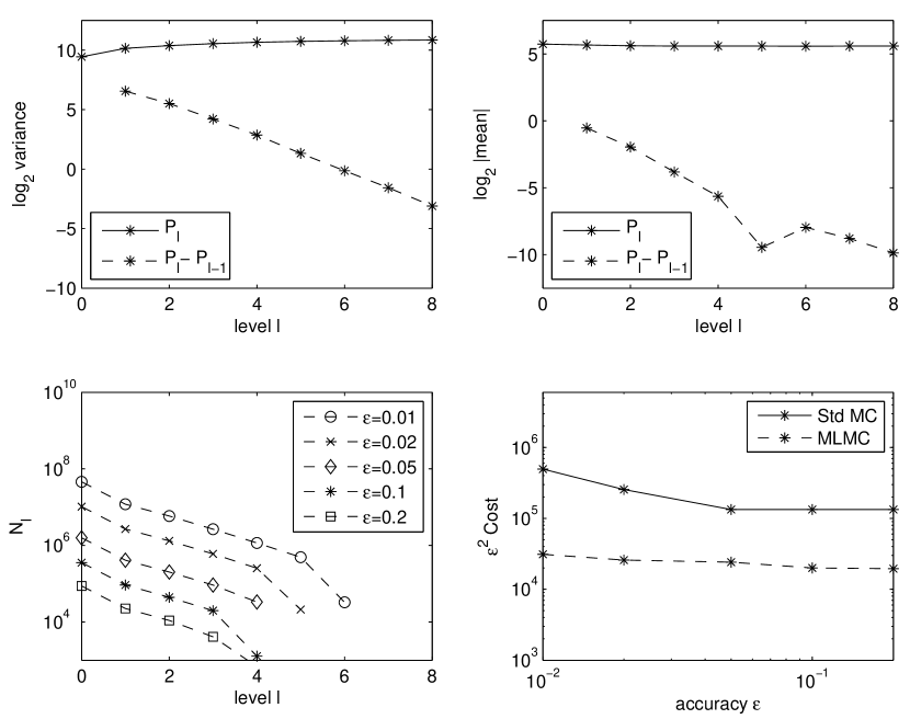
Figure 7: Digital option

In three cases, the conditional expectation of coarse-path estimator is equal to fine-path one, thus equality (6) is justified. Figure 6 clearly demonstrates three cases.

Figure 7 shows the numerical results for parameters $S(0)\!=\!100$, $K\!=\!100$, $T\!=\!1$, $r\!=\!0.05$, ${\sigma}\!=\!0.2$. The top left plot shows that the variance is approximately $O(h_{\ell}^{3/2})$, corresponding to $\beta\!=\!1.5$. The reason for this is similar to the argument in [Gil07].

A different feature compared to the geometric Brownian motion case is that the variance of the level 0 estimator is a constant increasing with jump rate $\lambda$, instead of zero. The reason is simply because that the trajectories in level 0 do vary in each simulation.

5 Path-dependent rate cases

In the case of path-dependent jump rates, which means the jump intensity depends on the process, for instance $\lambda=\lambda(S_{t},t)$, the implementation of multilevel becomes difficult due to the fact that path may jump at different time in the fine grid and coarse grid. These differences in path sample might enlarge the difference of quantities used in the computation of payoff between the fine grid and coarse grid, such as final payoff in vanilla and digital option, minimum estimator by Brownian bridge interpolation in lookback option and crossing probability in barrier option. This leads to a increased variance of every single splitted multilevel estimator and finally decrease the reduction of computation cost.

To tackle this obstacle, we propose two approaches. The first one facilitates the idea of change of measure in dealing with multilevel method for discontinuous payoffs, as we used before in dealing with digital option. The second one uses thinning technique to simulate the desired jump time with inhomogeneous rate through acceptance-rejection procedure. We again need to change the measure when evaluating $P_{\ell}-P_{\ell-1}$ in both grids to reduce variance.

5.1 Cumulative intensity method

In the first approach, which we call cumulative intensity method, we generate jump times from cumulative intensity which is computed in accordance with the dynamics evolution. We can see the idea from the case of deterministic time-inhomogeneous rate. For a time-inhomogeneous Poisson process whose instaneous intensity is $\lambda(s),$ the distribution of next jump time $\tau_{i+1}$ given $\tau_{i}$ is

$$P(\tau_{i+1}-\tau_{i}\leq t|\tau_{i})=1-\exp(-\int_{\tau_{i}}^{\tau_{i}+t}\lambda(s){\rm d}s).$$ (13)

construct jump-adapted schemes by approximating the instaneous jump rate adaptively with the evolution of the path sample at each time grid point. In other words, since jump intensity is path-dependent, the jump-adapted time discretisation grid should be generated corresponding to the evolution of the underlying process. In

In other words,

$$\int_{\tau_{i}}^{\tau_{i+1}}\lambda(s){\rm d}s\sim\mathcal{E}(1).\mbox{~{}(Exponential distribution with parameter 1.)}$$

We can use this property to generate $\tau_{i+1}$:

$$\Delta\tau_{i+1}=\inf\{{t\geq\tau_{i}:\int_{\tau_{i}}^{t}\lambda(s){\rm d}s\>>\mathcal{E}_{i+1}\}},~{}~{}\mathcal{E}_{i}\sim\mathcal{E}(1).$$

So

$$\tau_{i+1}=\tau_{i}+\Delta\tau_{i+1}.$$

If the cumulative intensity

$$\Lambda(t)=\int_{0}^{t}\lambda(s){\rm d}s$$

does not admit an explicit expression or it is computational intensive, we can use simple quadrature with linear interpolation to generate the approximated $\tau_{i+1}:$ $\ {\widehat{\tau}}_{i}$.

$$\int_{{\widehat{\tau}}_{i}}^{{\widehat{\tau}}_{i}+t_{n}}\lambda(s){\rm d}s\approx\sum_{i=1}^{n}\lambda_{i}h_{i}:=\Lambda_{n}$$

where $t_{n}$ is the next $n$th point in the fixed-timestep grid, $h_{i}$ is the timestep of the grid, $\lambda_{i}=\lambda({\widehat{\tau}}_{i}+\sum_{j=1}^{i-1}h_{j})$ is the instaneous intensity on the left endpoint of each timestep.

Let $N=\inf\{n:\Lambda_{n}>\mathcal{E}_{i+1}\}$, then

$$\Delta{\widehat{\tau}}_{i+1}=\dfrac{\mathcal{E}_{i+1}-\Lambda_{N-1}}{\lambda_{N}}$$ (14)

is a approximation of $\Delta\tau_{i+1}$.

In the case of random intensity where $\lambda$ only depends on current state, we can define $\tau_{i}$ as

$$\tau_{i}:=\inf{\large\{t:\int_{0}^{t}\lambda_{s}{\rm d}s\geq\mathcal{E}_{1}+\cdots+\mathcal{E}_{i}\}.}$$

We can use approximation of integral and (14) to generate ${\widehat{\tau}}_{i}$.

The algorithm of jump-adapted (Milstein) scheme with cumulative intensity would be:

    Algorithm (jump-adapted Milstein scheme with cumulative intensity)

Suppose that we have a fixed time grid constituted of $N$ timesteps, $t_{i}^{\prime}=i\times\frac{T}{N},~{}i=1,\ldots,N$.

1. Let $\Lambda,t,E=0,$ $i,\ j=1.\$Draw an exponential r.v. $\mathcal{E}_{j}$ with parameter 1;

2. While $t<T,$ do

   1. $\Lambda^{\prime}=\Lambda+\lambda({\widehat{S}}(t),t)(t_{i}^{\prime}-t),$ $E=\mathcal{E}_{j}+E,$

      1. If $\Lambda^{\prime}>\mathcal{E}_{j},$

         Let $h=\dfrac{\mathcal{E}_{j}-\Lambda}{\lambda({\widehat{S}}(t),t)},$ $\Lambda=E.$

         Mark ${\widehat{\tau}}_{j}=t+h$ as a jump time. Let $j=j+1$ and generate $\mathcal{E}_{j};$

      2. Otherwise $\Lambda=\Lambda^{\prime}.\ h=t_{i}^{\prime}-t;\ i=i+1.$

   2. (Use Milstein scheme) Simulate the evolution of the process from $t$ to $t+h,$ obtaining value of$\ {\widehat{S}}(t+h)$ depending on whether $t+h$ is a jump time.

      Let $t=t+h.$

As a side output, after the finishing of algorithm we have got the approximated jump times ${\widehat{\tau}}_{j}$, which combines $t_{i}^{\prime}=i\times\frac{T}{N},~{}i=1,\ldots,N$ forming jump-adapted grid $\mathbb{T}=\{0=t_{0}<t_{1}<t_{2}<\ldots<t_{M}=T\}.$

The point process ${\widehat{N}}_{t}$ corresponding to the stopping times ${\widehat{\tau}}_{i}$ is defined by

$${\widehat{N}}_{t}:=\sum_{i=1}^{\infty}{\mathbbm{1}}_{\{{\widehat{\tau}}_{i}\leq t\}}.$$ (15)

This process is indeed a point process with piecewise constant intensity $\lambda({\widehat{S}}(t_{k}),t_{k}),\ ~{}k=0,\ldots,M-1$ in $[t_{k},t_{k+1})$.

5.1.1 Multilevel treatment

When it comes to multilevel approach, the problem is that the current intensity may be different in fine and coarse grid, which leads to different distributions of next jump time. This causes two problems. First, we can no more use the random number generated for the path increment of fine grid to the one of the coarse grid, which is intrinsically unacceptable for multilevel approach. Secondly, the different final jumps may make a big difference between the payoffs in the fine grid and in the coarse grid, which is a similar challenge for digital option.

To handle these problems, we change the measure of Poisson rate in calculating the expectation in the coarse grid so that the distribution of next jump time agrees with the one in the fine grid. To do this let us first introduce the change of measure for Poisson processes (see section 9.3 of [CT04]).

Suppose $N_{t}\sim\mbox{Poi}(\lambda_{1})$ under some probability density $P_{1}$, then under probability density $P_{2}$ defined by

$$\dfrac{{\rm d}P_{2}}{{\rm d}P_{1}}=\exp((\lambda_{1}-\lambda_{2})t)(\dfrac{\lambda_{2}}{\lambda_{1}})^{N_{t}}$$ (16)

we will have $N_{t}\sim\mbox{Poi}(\lambda_{2})$, where the above term is called Radon-Nikodym derivative.

In the context of multilevel approach under state-dependent intensity model with jump-adapted scheme, we want to calculate

$$\mathbb{E}[{\widehat{P}}_{\ell}^{f}]-\mathbb{E}[{\widehat{P}}_{\ell-1}^{c}],$$

which we can rewrite as

$$\mathbb{E}[{\widehat{P}}_{\ell}^{f}-{\widehat{P}}_{\ell-1}^{f}{\widehat{R}}_{\ell}].$$

We shall explain the meaning of this formula: instead of defining in the jump-adapted grid formed by cumulative intensity approximated by coarse timestep $2h_{\ell},$ ${\widehat{P}}_{\ell-1}$ is defined in the jump-adapted grid formed by fine timestep $h_{\ell}$ approximation.

The Radon-Nikodym derivative ${\widehat{R}}_{\ell}$ is defined by

$${\widehat{R}}_{\ell}(T)=\dfrac{{\rm d}{\widehat{P}}_{c}}{{\rm d}{\widehat{P}}_{f}}=\exp(\Lambda_{\ell}^{f}-\Lambda_{\ell}^{c})\prod\limits_{k}\dfrac{\lambda_{k}^{c}}{\lambda_{k}^{f}},$$

in which $T$ is maturity, denoting $\lambda_{i}^{f}=\lambda({\widehat{S}}_{i}^{f},t_{i}),\lambda_{i}^{c}=\lambda({\widehat{S}}_{i}^{c},t_{i}),\ \Lambda_{\ell}^{f}=\sum_{i=1}^{n_{\ell}}\lambda_{i}^{f}h_{i}$ and $\Lambda_{\ell}^{c}=\sum_{i=1}^{n_{\ell}}\lambda_{i}^{c}h_{i}$ are approximated cumulative intensities upto the maturity in the fine and coarse grid, $k$ is the index that ${\widehat{\tau}}_{k+1}^{f}\$is the jump time, respectively.

This construction is valid since $\mathbb{E}[{\widehat{P}}_{\ell-1}^{c}]=\mathbb{E}[{\widehat{P}}_{\ell-1}^{f}{\widehat{R}}_{\ell}],$ which can be seen as a piecewise constant extension of (16). This can be justified by the theorem 2.31 in Chapter 2 of [Kar91]. Detail will be done in the future work.

5.1.2 Variance convergence order

In the following we shall give some intuitive analysis of the variance convergence order, which is not a rigorous proof. Hopefully we can use extreme path theory to prove it thoroughly in the future work.

The variance of estimator ${\widehat{P}}_{\ell}^{(j)}-{\widehat{P}}_{\ell-1}^{(j)}{\widehat{R}}_{\ell}^{(j)}$ is

$${\mathbb{V}}[{\widehat{P}}_{\ell}-{\widehat{P}}_{\ell-1}{\widehat{R}}_{\ell}] = {\mathbb{V}}[{\widehat{P}}_{\ell}-{\widehat{P}}_{\ell-1}+{\widehat{P}}_{\ell-1}(1-{\widehat{R}}_{\ell})]$$

$$\leq \left[\left({\mathbb{V}}[{\widehat{P}}_{\ell}-{\widehat{P}}_{\ell-1}]\right)^{\frac{1}{2}}+\left({\mathbb{V}}[{\widehat{P}}_{\ell-1}(1-{\widehat{R}}_{\ell})]\right)^{\frac{1}{2}}\right]^{2}.$$

The first part has the order of $O(h\dot{)}$. To see the order of ${\widehat{R}}_{\ell}$, let us examine the asymptomatic order of squared variance of two components of ${\widehat{R}}_{\ell}$: the exponential part and product part alternatively:

$${\widehat{R}}_{\ell}=\exp\left[\sum_{i=1}^{n_{\ell}}(\lambda_{i}^{f}-\lambda_{i}^{c})h_{i}\right]\prod\limits_{k}\dfrac{\lambda_{k}^{c}}{\lambda_{k}^{f}}.$$

where $\lambda_{i}^{f}=\lambda({\widehat{S}}_{i}^{f},t_{i}),\lambda_{i}^{c}=\lambda({\widehat{S}}_{i}^{c},t_{i}).$

We will concentrate on the effect caused in midpoint interval.

Let $h$ be the timestep of uniform fine grid. Given a midpoint interval $[t_{j},t_{j+2}]$, since by definition $\lambda_{j+1}^{c}=\lambda_{j}^{c}$, the exponential part for $[t_{j},t_{j+2}]$ is

$$\sum_{i=j}^{j+1}(\lambda_{i}^{f}-\lambda_{i}^{c})h_{i} = (\lambda_{j}^{f}-\lambda_{j}^{c})(h_{j}+h_{j+1})+(\lambda_{j+1}^{f}-\lambda_{j}^{f})h_{j+1}$$

$$\sim O(h)h+\frac{\partial\lambda}{\partial S}({\widehat{S}}(t_{j})^{f},t_{j})({\widehat{S}}_{j+1}^{f}-{\widehat{S}}_{j}^{f})h$$

$$\sim O(h^{3/2}).$$

The first term is implied by $O(h)$ strong convergence and second one comes from ${\widehat{S}}_{j+1}^{f}-{\widehat{S}}_{j}^{f}\sim{\widehat{S}}_{j}^{f}\triangle W_{h_{j+1}}\sim O(h^{1/2})$.

Summing all intervals in the grid, since there are $N=T/2h$ midpoint intervals, and the rest contributes higher order, asymptotically we get $\sum_{i=1}^{n_{\ell}}(\lambda_{i}^{f}-\lambda_{i}^{c})h_{i}\sim O(h)$. Thus the exponential part satisfies

$$\exp\left[\sum_{i=1}^{n_{\ell}}(\lambda_{i}^{f}-\lambda_{i}^{c})h_{i}\right]\sim 1+O(h).$$

For the product part, when $t_{j+2}$ is a jump time, by similar argument it holds that :

$$\frac{\lambda_{j+1}^{f}}{\lambda_{j+1}^{c}} = 1+\frac{\lambda_{j}^{f}-\lambda_{j}^{c}+\lambda_{j+1}^{f}-\lambda_{j}^{f}}{\lambda_{j}^{c}}$$

$$\sim 1+O(h^{1/2}).$$

So the product part satisfies

$$\prod\limits_{k}\dfrac{\lambda_{k}^{c}}{\lambda_{k}^{f}}\sim 1+O(h^{1/2}).$$

Asymptotically we get

$${\mathbb{V}}\left[{\widehat{R}}_{\ell}\right]=O(h).$$

Therefore we have evidence to support that the variance convergence order for the multilevel estimator should be

$${\mathbb{V}}[{\widehat{P}}_{\ell}-{\widehat{P}}_{\ell-1}{\widehat{R}}_{\ell}]=O(h).$$

Although cumulative intensity method can deal with the case where jump rate is not bounded, the variance convergence order $O(h)$ leads to a computational complexity of $O(\varepsilon^{-2}\left(\log\varepsilon\right)^{2})$.

5.2 Thinning method

The idea of the thinning method is to construct a Poisson process with a constant rate $\lambda_{\sup}$ which is an upper bound of the state-dependent rate. This gives a set of candidate jump times, and these are then selected as true jump times with probability $\lambda(S_{t},t)/\lambda_{\sup}$.

5.2.1 Algorithm

Suppose that we have simulated the jump time grid $\mathbb{J}=\{\tau_{1},\tau_{2},\ldots,\tau_{m}\}$ generated by a Poisson process with constant rate $\lambda_{\sup}$, which includes times at which jumps occur in $[0,T]$. On the other hand, consider a fixed time grid constituted of $N$ timesteps, $t_{i}^{\prime}=i\times\frac{T}{N},~{}i=1,\ldots,N,$ which is used in discretisation schemes for diffusive SDEs. Now the superposition of them will be a jump-adapted thinning grid $\mathbb{T}=\{0=t_{0}<t_{1}<t_{2}<\ldots<t_{M}=T\}$.

For a process which we can simulate the exact increments we have the following thinning procedure:

1. Generate the waiting time for next jump time $\tau_{i+1}-\tau_{i}$ from a Poisson process with constant rate $\lambda_{\sup}$;

2. Simulate the evolution of the process up to time $\tau_{i+1}$;

3. Draw a uniform random number $U\sim[0,1]$,

   1. If $p=\dfrac{\lambda(S(\tau_{i+1}-),\tau_{i+1})}{\lambda_{\sup}}>U$, accept $\tau_{i+1}$ as a real jump time and simulate the jump; otherwise go to 2.

For the general processes we use certain discretisation scheme, e.g. we have the following jump-adapted thinning (Milstein) scheme:

1. Generate the jump-adapted time grid for a Poisson process with constant rate $\lambda_{\sup}$;

2. Simulate each timestep using the (Milstein) discretisation;

3. When the endpoint $t_{n+1}$ is a candidate jump time, generate a uniform random number $U\sim[0,1]$, and if $U<p_{\tau}=\dfrac{\lambda(S(\tau-),\tau)}{\lambda_{\sup}}$, then accept $t_{n+1}$ as a real jump time and simulate the jump.

If we look from the perspective of random measure notation, the thinning method can also be formulated in the following ways. First let us recall some definitions of point processes and random measures.

5.2.2 Point processes and random measures

There are two kinds of basic stochastic processes. The path evolution of the first kind is driven by continuous increment, while in the second kind the path will only change in the certain jump times. In order to describe the stochastic processes of discrete paths, we need to introduce point process.

Given a filtered probability space $(\Omega,\mathcal{F}_{t},\mathbb{P})$, if we have a increasing sequence of increasing stopping times

$$0=T_{0}<T_{1}<T_{2}<\ldots$$

and

$$\lim_{n\rightarrow\infty}T_{n}=\infty,$$

then the point (counting) process $N_{t}$ associated with stopping times (jump times) is defined as

$$N_{t}=\sum_{n\geq 1}1_{\{T_{n}<t\}}.$$

It counts the number of jumps up to time $t$. To depict the jump amplitude (mark) at each jump time, we can define marked point processes and associated random measure.

Suppose mark $Y_{n}$ are random variables taking values on a mark space $E\subseteq R^{r}\backslash\left\{0\right\}$, and $Y_{n}$ are $\mathcal{F}_{T_{n}}$ measurable, then $(Y_{n},T_{n})$ is called a marked point process on  $E\times[0,\infty].$

For any $A\subseteq B(E)$ and any $\omega\in\Omega$,

$$\mu(\omega;[0,t),A):=\sum_{n\geq 1}1_{\{T_{n}\left(\omega\right)<t\}}1_{\{Y_{n}\left(\omega\right)\in A\}}$$

defines the random measure associated with marked point process $(Y_{n},T_{n})$. It counts the number of jumps within $[0,t)$ whose amplitude belonging to $A$. The class of marked point process is quite general, actually it is a bijection to the class of càdlàg process.

For each $\omega\in\Omega$, $\mu\left(\omega;\cdot,\cdot\right)$ is an Radon measure on $\left(E\times[0,\infty],\mathcal{\ B}\left(E\times[0,\infty]\right)\right).$ Thus for each $\mathbb{P}$-measuable  function $f$, the integral

$$\int_{E\times[0,t]}f(\omega;z,s)\mu(\omega;{\rm d}z,{\rm d}s):=\sum_{\begin{subarray}{c}n\geq 1\\ T_{n}\left(\omega\right)<t\end{subarray}}f\left(Y_{n}\left(\omega\right),T_{n}\left(\omega\right)\right)$$

is a well-defined random variable.

The compensator $\varphi({\rm d}z){\rm d}s$ of the random measure is defined so that for all bounded $\mathbb{P}$-measurable  function $f,$ we have

$$\int_{0}^{t}\int_{z\in E}f(z,s)\mu({\rm d}z,{\rm d}s)-\int_{0}^{t}\int_{z\in E}f(z,s)\varphi({\rm d}z){\rm d}s$$

is a martingale with respect to $\mathcal{F}_{t}$.

Following the assumption of Platen, we assume that $\int_{z\in E}\varphi({\rm d}z)<\infty$ for all $s>0$.

Under those notations, (2) can be rewritten as:

$${\rm d}S(t)=a(S(t-),t){\rm d}t+b(S(t-),t){\rm d}W(t)+c(S(t-),t)\int_{z\in E}(z-1)p_{\lambda}({\rm d}z,{\rm d}t),\quad 0\leq t\leq T.$$

where $p_{\lambda}\left(\omega;\cdot,\cdot\right)$ is a Poisson random measure, which means the compensator $\varphi({\rm d}z)=\lambda g(z){\rm d}z$ is time independent and $g(z)$ is p.d.f of the mark . In this case the waiting time $T_{n+1}-T_{n}$ is exponential distributed with a parameter $\lambda$.

Those general definitions are to allow more flexibility of the dynamics of SDEs, e.g. it can admit state-dependent intensity. The dynamics of the state-dependent jump-diffusion SDEs we will deal with can be written as

$${\rm d}S(t)=a(S(t-),t){\rm d}t+b(S(t-),t){\rm d}W(t)+\int_{z\in E}c(S(t-),t,z)\mu({\rm d}z,{\rm d}t),\quad 0\leq t\leq T.$$ (17)

The compensator of $\mu$ is defined to be $\varphi(S(t-),{\rm d}z)\lambda(S(t-),t)g(z){\rm d}z.$ We also adopt the assumption in [GM04] that it is bounded by a constant $\lambda_{\sup}$ and is absolutely continuous.

The jump-adapted thinning Milstein scheme for (17) can be formulated as

$${\widehat{S}}_{n+1}^{-} = {\widehat{S}}_{n}+a_{n}\,h_{n}+b_{n}\,\Delta W_{n}+{\textstyle\frac{1}{2}}\,b_{n}^{\prime}b_{n}\,(\Delta W_{n}^{2}-h_{n}),$$

$${\widehat{S}}_{n+1} = {\widehat{S}}_{n+1}^{-}+\int_{z\in E}1_{\{\frac{\lambda({\widehat{S}}_{n+1}^{-},t_{n+1})}{\lambda_{\sup}}>U_{i}\}}c({\widehat{S}}_{n+1}^{-},t_{n+1},z)\mu({\rm d}z,t_{n+1}).$$

5.2.3 Multilevel treatment

In the multilevel implementation, if we use the above algorithm with different acceptance probabilities for fine and coarse level, there may be some samples in which a jump candidate is accepted for the fine path, but not for the coarse path, or vice versa. Because of first order strong convergence, the difference in acceptance probabilities will be $O(h)$, and hence there is an $O(h)$ probability of coarse and fine paths differing in accepting candidate jumps. Such differences will give an $O(1)$ difference in the payoff value, and hence the multilevel variance will be $O(h)$. A more detailed analysis of this is given in [XG11].

To improve the variance convergence rate, we use a change of measure so that the acceptance probability is the same for both fine and coarse paths. This is achieved by taking the expectation with respect to a new measure $Q$:

$${\mathbb{E}}[{\widehat{P}}_{\ell}-{\widehat{P}}_{\ell-1}]={\mathbb{E}}_{Q}[{\widehat{P}}_{\ell}\prod_{\tau}R_{\tau}^{f}-{\widehat{P}}_{\ell-1}\prod_{\tau}R_{\tau}^{c}]$$

where $\tau$ are the jump times. The acceptance probability for a candidate jump under the measure $Q$ is defined to be $\frac{1}{2}$ for both coarse and fine paths, instead of $p_{\tau}=\lambda(S(\tau-),\tau)\,/\,\lambda_{\sup}$. The corresponding Radon-Nikodym derivatives are

$$R_{\tau}^{f}=\left\{\begin{aligned} &2p_{\tau}^{f},~{}&\mbox{if}~{}U<\frac{1}{2}&~{};\\ &2(1-p_{\tau}^{f}),~{}&\mbox{if}~{}U\geq\frac{1}{2}&~{},\end{aligned}\right.\quad\quad R_{\tau}^{c}=\left\{\begin{aligned} &2p_{\tau}^{c},~{}&\mbox{if}~{}U<\frac{1}{2}&~{};\\ &2(1-p_{\tau}^{c}),~{}&\mbox{if}~{}U\geq\frac{1}{2}&~{},\end{aligned}\right.$$

Since $R_{\tau}^{f}-R_{\tau}^{c}=O(h)$ and ${\widehat{P}}_{\ell}-{\widehat{P}}_{\ell-1}=O(h)$, this results in the multilevel correction variance ${\mathbb{V}}_{Q}[{\widehat{P}}_{\ell}\prod_{\tau}R_{\tau}^{f}-{\widehat{P}}_{\ell-1}\prod_{\tau}R_{\tau}^{c}]$ being $O(h^{2})$.

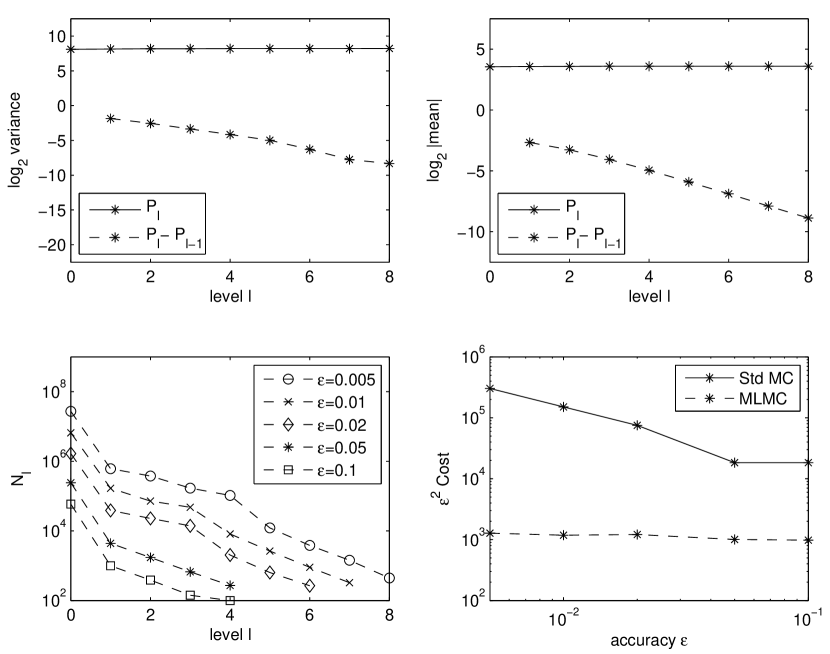
Figure 8: European call option with path-dependent Poisson rate using thinning without a change of measure

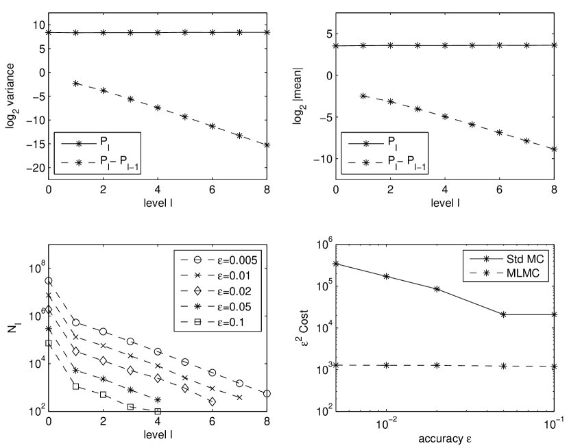
Figure 9: European call option with path-dependent Poisson rate using thinning with a change of measure

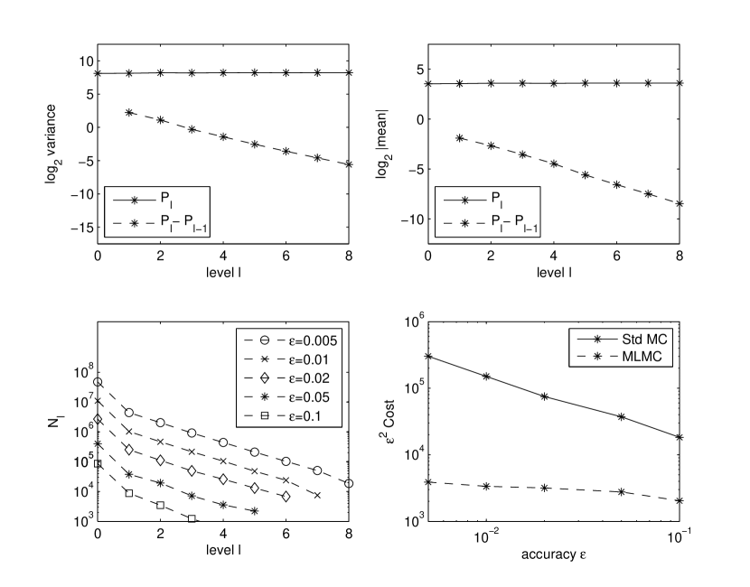
Figure 10: European call option with path-dependent Poisson rate using cumulative intensity method

The weak convergence of the jump-adapted discretisation with the thinning procedure is proved in [GM04], for a class of payoffs on which they impose to be $4$th differentiable and that its up to 4th order partial derivatives are uniformly bounded. By Stone–Weierstrass theorem we can construct a sequence of smoothing polynomials which uniformly converges to continuous payoff. The limits of this approach is that it is invalid for discontinuous payoffs. To prove the convergent variance of multilevel estimator, assuming the Lipschitz condition on $\lambda$, we decompose the estimator into the constant rate part and the Randon-Nikdym derivative part, disentangling the effect of path-dependence of intensity from the estimator. Under such assumption, we can obtain the weak convergence of the estimators for various payoffs by the same decomposition, circumventing the difficulties caused by discontinuous payoffs. The advantage of this argument is that it can reduce the analysis to the constant rate case so that the proof is simplified.

If the analytic formulation is expressed using the same thinning and change of measure, the weak error can be decomposed into two terms as follows:

$${\mathbb{E}}_{Q}\left[{\widehat{P}}_{\ell}\prod_{\tau}R_{\tau}^{f}-P\prod_{\tau}R_{\tau}\right]\ =\ {\mathbb{E}}_{Q}\left[({\widehat{P}}_{\ell}-P)\ \prod_{\tau}R_{\tau}^{f}\right]\ +\ {\mathbb{E}}_{Q}\left[P\ (\prod_{\tau}R_{\tau}^{f}-\prod_{\tau}R_{\tau})\right].$$

Using Hölder’s inequality, the bound $\max(R_{\tau},R_{\tau}^{f})\leq 2$ and standard results for a Poisson process, the first term can be bounded using weak convergence results for the constant rate process, and the second term can be bounded using the corresponding strong convergence results [XG11]. This guarantees that the multilevel procedure does converge to the correct value.

5.2.4 Numerical results

We show numerical results for a European call option using the underlying dynamics under risk-neutral measure:

$$\dfrac{{\rm d}S(t)}{S(t-)}=r\,{\rm d}t+{\sigma}\,{\rm d}W(t)++\int_{z\in E}z\mu({\rm d}z,{\rm d}t)-\int_{z\in E}zf(z){\rm d}z\lambda{\rm d}t,\quad 0\leq t\leq T,$$

where the random measure $\mu$ has compensator $\lambda{\rm d}t$ with $\lambda=\frac{1}{1+(S(t-)/S_{0})^{2}}$.   The mark has a $\log$ normal distribution the density function of which is denoted by $f(z)$.

We use $\lambda_{\sup}=1$ to generate thinning process. All other parameters as used previously for the constant rate cases.

Comparing Figures 8 and 9 we see that the variance convergence rate is significantly improved by the change of measure, but there is little change in the computational cost. This is due to the main computational effort being on the coarsest level, which suggests using quasi-Monte Carlo on that level [GW09].

The bottom left plot in Figure 8 shows a slightly erratic behaviour. This is because the $O(h_{\ell})$ variance is due to a small fraction of the paths having an $O(1)$ value for ${\widehat{P}}_{\ell}-{\widehat{P}}_{\ell-1}$. In the numerical procedure, the variance is estimated using an initial sample of 100 paths. When the variance is dominated by a few outliers, this sample size is not sufficient to provide an accurate estimate, leading to this variability.

For comparison, we also show the numerical result given by cumulative intensity method in Figure 10. The bottom left plot indicates the $O(h_{\ell})$ variance and the rest plots can be understood consequently.

6 Conclusions

In this work we extend the Multilevel approach to scalar jump-diffusion SDEs using jump-adapted schemes. The second order variance convergence is maintained in the constant rate case, by constructing estimators using a previous Brownian interpolation technique. In the state-dependent rate case, we use thinning with a change of measure to avoid the asynchronous jumps in the fine and coarse levels. We have also investigated an alternative approach which can handle cases in which there is no upper bound on the jump rate.

The first natural future work is to do rigorous numerical analysis on the convergence of variance of correction terms, and weak convergence of the ML estimators, which is work in progress [XG11]. The second direction is to investigate other cases of model based on specific infinite activity Lévy processes, e.g. variance gamma. We also plan to investigate whether the multilevel quasi-Monte Carlo method will further reduce the cost.

References

- [BLP05] Nicola Bruti-Liberati and Eckhard Platen. On the strong approximation of jump-diffusion processes. technical report, QFRC research paper 157, University of Technology, Sydney, 2005.
- [CT04] R. Cont and P. Tankov. Financial modelling with jump processes. Chapman & Hall, 2004.
- [Der11] S. Dereich. Multilevel Monte Carlo Algorithms for Lévy-driven SDEs with Gaussian Correction. The Annals of Applied Probability, 21(1):283–311, 2011.
- [DH11] S. Dereich and F. Heidenreich. A multilevel monte carlo algorithm for lévy-driven stochastic differential equations. Stochastic Processes and their Applications, 121(7):1565–1587, 2011.
- [Gil07] M.B. Giles. Improved multilevel Monte Carlo convergence using the Milstein scheme. In A. Keller, S. Heinrich, and H. Niederreiter, editors, Monte Carlo and Quasi-Monte Carlo Methods 2006, pages 343–358. Springer-Verlag, 2007.
- [Gil08a] M.B. Giles. An extended collection of matrix derivative results for forward and reverse mode algorithmic differentiation. Technical Report NA08/01, Oxford University Computing Laboratory, 2008.
- [Gil08b] M.B. Giles. Multilevel Monte Carlo path simulation. Operations Research, 56(3):607–617, 2008.
- [Gla04] P. Glasserman. Monte Carlo Methods in Financial Engineering. Springer, New York, 2004.
- [GM03] P. Glasserman and N. Merener. Numerical solution of jump-diffusion LIBOR market models. Finance and Stochastics, 7(1):1–27, 2003.
- [GM04] P. Glasserman and N. Merener. Convergence of a discretization scheme for jump-diffusion processes with state-dependent intensities. Proc. Royal Soc. London A, 460:111–127, 2004.
- [GW09] M.B. Giles and B.J. Waterhouse. Multilevel quasi-Monte Carlo path simulation. Advanced Financial Modelling, page 165, 2009.
- [Hei01] S. Heinrich. Multilevel Monte Carlo Methods, volume 2179 of Lecture Notes in Computer Science, pages 58–67. Springer-Verlag, 2001.
- [Kar91] Alan F. Karr. Point Processes And Their Statistical Inference. Second edition, 1991.
- [Keb05] A. Kebaier. Statistical Romberg extrapolation: a new variance reduction method and applications to options pricing. Annals of Applied Probability, 14(4):2681–2705, 2005.
- [Mer76] R.C. Merton. Option pricing when underlying stock returns are discontinuous. Journal of Financial Economics, 3(1-2):125–144, 1976.
- [Pla82] E. Platen. A generalized Taylor formula for solutions of stochastic equations. Sankhyā: The Indian Journal of Statistics, Series A, 44(2):163–172, 1982.
- [Pla10] N. Platen, E.and Bruti-Liberati. Numerical Solution of Stochastic Differential Equations with Jumps in Finance, volume 64 of Stochastic Modelling and Applied Probability. Springer-Verlag, 1st edition, 2010.
- [XG11] Y. Xia and M.B. Giles. Numerical analysis of multilevel Monte Carlo for scalar jump-diffusion SDEs. working paper in preparation, 2011.