Low temperature properties of the infinite-dimensional attractive Hubbard model

Abstract

We investigate the attractive Hubbard model in infinite spatial dimensions by combining dynamical mean-field theory with a strong-coupling continuous-time quantum Monte Carlo method. By calculating the superfluid order parameter and the density of states, we discuss the stability of the superfluid state. In the intermediate coupling region above the critical temperature, the density of states exhibits a heavy fermion behavior with a quasi-particle peak in the dense system, while a dip structure appears in the dilute system. The formation of the superfluid gap is also addressed.

I Introduction

Ultracold atomic systems have attracted a lot of interest following the demonstration of Bose-Einstein condensation (BEC) in a Rb atom system Rb . Among the many interesting issues, the nature of the superfluid state in fermionic systems Regal is a widely studied topic, since a crossover between a weak-coupling BCS-type superfluid state and a strong-coupling BEC-type superfluid state (BCS-BEC crossover) has been observed in experiments BCSBEC1 ; BCSBEC2 ; BCSBEC3 . Recently, the appearance of a pseudogap in the density of states has also been suggested JILA , which stimulates further theoretical investigations on the superfluid state and related phenomena.

Fermi gas systems have been studied theoretically in much detail and it has been clarified that a pseudogap phenomenon indeed appears in the BCS-BEC crossover region above the critical temperature Chen ; Tsuchiya ; Chien ; Su . More recently, the gap structure in the superfluid state has been discussed Pieri ; Watanabe . It has been pointed out that upon decreasing temperature, the pseudogap disappears at a certain temperature inside the superfluid phase and the superfluid gap opens instead Watanabe . On the other hand, in fermionic optical lattice systems described by the attractive Hubbard model, such dynamical properties at finite temperatures have not been discussed. It is also important to clarify how the particle density as well as the interaction strength affect the low energy properties in the pseudogap region. Therefore, it is useful to study the stability of the superfluid state systematically and to clarify how the gap structure appears in the density of states at low temperatures.

In this paper, we consider the infinite-dimensional attractive Hubbard model to discuss its low temperature properties. To take correlation effects precisely into account, we combine dynamical mean-field theory (DMFT) Metzner ; Muller ; Georges ; Pruschke with a continuous-time quantum Monte Carlo (CTQMC) method solver_review . This unbiased technique enables us to discuss the stability of the superfluid state quantitatively. By tuning the particle density, interaction strength, and temperature, we determine phase diagrams of the system and discuss the formation of the gap in the density of states.

The paper is organized as follows. In §2, we introduce the attractive Hubbard model and briefly summarize our theoretical approach. We discuss how the superfluid state is realized at low temperatures in §3. In §4, we focus on the dilute system in the BCS-BEC crossover region. We clarify how the gap structure appears in the density of states and discuss the difference of low energy properties in lattice and Fermi gas systems. A brief summary is given in the last section.

II Model and Method

We consider two-component fermions in an optical lattice, which may be described by the following Hubbard Hamiltonian,

$$\hat{\cal{H}}=-t\sum_{(i,j),\sigma}c^{\dagger}_{i\sigma}c_{j\sigma}-U\sum_{i}n_{i\uparrow}n_{i\downarrow},$$ (1)

where $c_{i\sigma}$ ($c^{\dagger}_{i\sigma}$) is an annihilation (creation) operator of a fermion on the $i$th site with spin $\sigma(=\uparrow,\downarrow)$, and $n_{i\sigma}=c^{\dagger}_{i\sigma}c_{i\sigma}$. $U$ is the onsite attractive interaction and $t$ is the transfer integral between sites. The low-energy properties of the attractive Hubbard model have been studied in one dimension Lieb ; Shiba ; Machida ; Xianlong ; Pour ; Fujihara , two dimensions TD1 ; TD2 ; Koga and infinite dimensions Garg ; Toschi ; Suzuki ; Keller ; Capone ; Bauer ; Freericks ; Privitera ; KogaQMC1 . It is known that the superfluid ground state is always realized in two and higher dimensions, where the BCS-BEC crossover has been studied in detail. However, dynamical properties have not been studied yet in detail in the intermediate correlation and temperature region. In particular, the question whether and how a pseudogap appears in the density of states above the critical temperature, has not been answered. In this paper, we systematically investigate the low temperature properties in the attractive Hubbard model by varying the particle density, interaction strength, and temperature. We then clarify how the gap structure appears in the density of states.

For this purpose, we make use of DMFT Metzner ; Muller ; Georges ; Pruschke . In DMFT, the original lattice model is mapped to an effective impurity model, where local particle correlations are accurately taken into account. The lattice Green’s function is obtained via a self-consistency condition imposed on the impurity problem. This treatment is exact in infinite dimensions, and the DMFT method has successfully been applied to strongly correlated fermion systems. In DMFT, we take into account dynamical correlations through the frequency-dependent self-energy. This allows us to discuss the stability of the $s$-wave superfluid state more quantitatively than in the static BCS mean-field theory.

The lattice Green’s function is given by

$$\hat{G}^{-1}(k,i\omega_{n})=i\omega_{n}\hat{\sigma}_{0}+\left(\mu-\epsilon_{k}\right)\hat{\sigma}_{z}-\hat{\Sigma}\left(i\omega_{n}\right),$$ (2)

where $\mu$ is the chemical potential, $\hat{\sigma}_{0}$ and $\hat{\sigma}_{z}$ are the identity matrix and the $z$-component of the Pauli matrix, $\epsilon_{k}$ is the dispersion relation for the non-interacting system, and $\omega_{n}$ is the Matsubara frequency. $\hat{\Sigma}(i\omega_{n})$ is the local self-energy in the Nambu formalism. The local lattice Green’s function is obtained as

$$\hat{G}(i\omega_{n})=\int dk\hat{G}(k,i\omega_{n}).$$ (3)

In this paper, we use a semi-circular density of states, $\rho(x)=2/\pi D\sqrt{1-(x/D)^{2}}$, where $D$ is the half bandwidth, which corresponds to an infinite coordination Bethe lattice. The self-consistency equation GeorgesZ is then given by

$$\hat{G}_{0,\text{imp}}^{-1}(i\omega_{n})=i\omega_{n}\hat{\sigma}_{0}+\mu\hat{\sigma}_{z}-\left(\frac{D}{4}\right)^{2}\hat{\sigma}_{z}\hat{G}(i\omega_{n})\hat{\sigma}_{z}.$$ (4)

There are various numerical methods to solve the effective impurity problem. To study the attractive Hubbard model systematically, an unbiased and accurate numerical solver is necessary, such as the exact diagonalizationCaffarel ; Toschi ; Privitera or the numerical renormalization group NRG ; NRG_RMP ; OSakai ; Bauer . A particularly powerful method for exploring finite temperature properties is CTQMC solver_review . In our previous paper KogaQMC1 , we have used the CTQMC method in the continuous-time auxiliary field formulation CTAUX to study the imbalanced attractive Hubbard model. However, this is a weak-coupling approach, which is not suitable for a systematic investigation of the low-temperature properties in the strong coupling regime. Hence, our previous discussion was restricted to the weak coupling region. Here, we employ the complementary strong coupling version of the CTQMC method CTQMC , which is more efficient in the large $|U|$ region. We use this method to investigate the attractive Hubbard model both in the weak and strong coupling regimes. Some details of the implementation are explained in the appendix.

In this paper, we use the half bandwidth $D$ as the unit of energy. We then calculate the pair potential $\Delta$, double occupancy $d$, internal energy $E$, and specific heat $C$, which are given Toschi by

$$\Delta = \langle c_{i\uparrow}c_{i\downarrow}\rangle=\hat{G}_{12}(\tau=0_{+}),$$ (5)

$$d = \langle n_{i\uparrow}n_{i\downarrow}\rangle,$$ (6)

$$E = \left(\frac{D}{2}\right)^{2}\int_{0}^{\beta}d\tau{\rm Tr}\left[\hat{G}(\tau)\hat{\sigma}_{z}\hat{G}(-\tau)\hat{\sigma}_{z}\right]+Ud,$$ (7)

$$C = \frac{dE}{dT}.$$ (8)

In addition to these static quantities, we deduce the density of states by applying the maximum entropy method MEM1 ; MEM2 ; MEM3 to the Green’s function. We then discuss how the gap structure appears in the system.

III Stability of the superfluid state

We first consider the attractive Hubbard model with different band fillings to discuss how the superfluid state is realized at low temperatures Toschi ; Privitera ; Bauer ; Garg . Figure 1 shows the pair potential $\Delta$ and the double occupancy $d$ at a fixed temperature $T=0.02$.

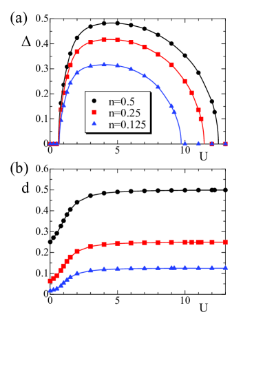
Figure 1: Pair potential (a) and double occupancy (b) as a function of the interaction at temperature $T=0.02$. Circles, squares, and triangles show the results for the system with $n=0.5$, $0.25$ and $0.125$, respectively.

In the noninteracting case $(U=0)$, a normal metallic state is realized, with $\Delta=0$ and $d=n^{2}$. Attractive interactions lead to the formation of Cooper pairs and an increase in the double occupancy, as shown in Fig. 1 (b). More precisely, at a certain critical interaction $U_{c1}$, a phase transition occurs to a superfluid state and the pair potential is induced, as shown in Fig. 1 (a). A cusp singularity appears in the curve of the double occupancy although it is not visible on this scale.

To clarify how the phase transition affects dynamical properties, we show the density of states deduced by the MEM in Fig. 2.

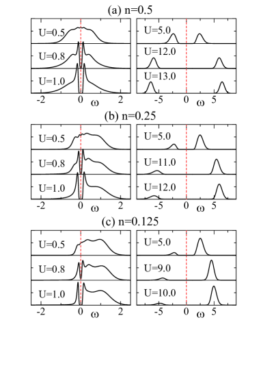
Figure 2: Density of states for the systems with $n=0.5$ (a), $0.25$ (b) and $0.125$ (c) at $T=0.02$.

When $U<U_{c1}$, the system is metallic with a finite density of states around the Fermi level. If the system enters the superfluid state, weakly coupled Cooper pairs are formed, which give rise to a tiny superfluid gap together with coherence peaks at its edges. This characteristic behavior is found for all the band fillings considered, so we can say that a BCS-type superfluid state is realized in the region $(U\sim 1)$. By examining the critical behavior of the pair potential, we deduce $U_{c1}\sim 0.62,0.64$ and $0.68$ for $n=0.5,0.25$ and $0.125$, respectively.

When $U\sim 5$, the pair potential has a maximum and the double occupancy approaches the particle density $(d\sim n)$, as shown in Fig. 1. This means that most fermions are tightly coupled to form paired bosons, which stabilizes the superfluid ground state. In this case, the energy scale should be $t^{2}/U$, characteristic of the hopping for the paired bosons. Therefore, a further increase in the attractive interaction effectively increases the temperature of the system, making the superfluid state unstable. Eventually, the pair potential vanishes and a phase transition occurs to the normal state at another critical point $U_{c2}$, as shown in Fig. 1 (a). In contrast to the BCS region, a large gap remains in the density of states and the phase transition little affects its features, as shown in Fig. 2. This originates from the fact that in the region $(U\gtrsim 5)$, paired bosons exist in the normal state as well as in the superfluid state. Therefore, we conclude that a BEC-type superfluid state, which can be regarded as the condensation of paired bosons, is stabilized at low temperatures. The critical values are obtained as $U_{c2}\sim 12.5,11.4$ and $9.7$ for $n=0.5,0.25$ and $0.125$.

In the superfluid phase, the BCS-type state $(U\sim 1)$ is adiabatically connected to the BEC-type one $(U\gtrsim 5)$. A BCS-BEC crossover thus occurs between the two states. Figure 3 shows the temperature dependence of the pair potential for three cases with $U=1,2$ and $5$.

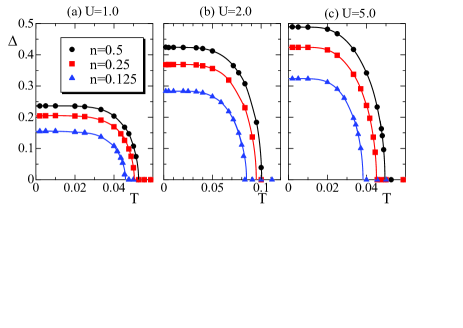
Figure 3: Pair potential as a function of temperature in systems with $U=1.0$ (a), $2.0$ (b), and $5.0$ (c). Circles, squares, and triangles represent the results for the systems with $n=0.5$, $0.25$ and $0.125$, respectively.

When the temperature is decreased, the pair potential is induced at the critical temperature, where the phase transition occurs from the normal state to the superfluid state. We find that the pair potential increases monotonically with decreasing temperature and saturates at low temperatures $(T\lesssim 0.01)$. Extrapolating the pair potential to zero temperature $\Delta_{T=0}$, we also deduce the quantity $q=U\Delta_{T=0}/T_{c}$, as shown in Fig. 4.

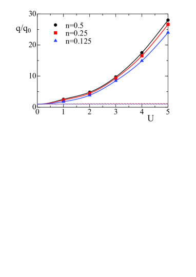
Figure 4: The ratio $q/q_{0}$ as a function of the interaction $U$. $q_{0}$ is the universal value in the weak-coupling limit obtained from the BCS theory. Circles, squares, and triangles represent the results for the system with $n=0.5$, $0.25$ and $0.125$, respectively.

In the weak coupling limit ($U\rightarrow 0$), a BCS-type superfluid state is realized, where this quantity is independent of the band filling and takes the universal value $q_{0}=1.764$, according to the simple BCS mean-field theory. Increasing the interaction strength, $q$ monotonically increases, in a way which depends on the band filling. In the strong coupling region, the quantity is proportional to the square of the interaction strength $q\sim U^{2}$ since the pair potential $\Delta_{T=0}$ should saturate and $T_{c}\sim 1/U$. We note that these results differ considerably from those obtained by the simple BCS mean-field theory, where quantum fluctuations are not taken into account properly. In fact, the critical temperature is always overestimated (as shown in Fig. 5) and $q_{BCS}$ is almost constant, as shown by the dashed lines in Fig. 4. Therefore, it is crucial to take into account dynamical correlations correctly in the attractive Hubbard model with $U\gtrsim 1$.

By performing similar calculations, we determined the phase diagram shown in Fig. 5.

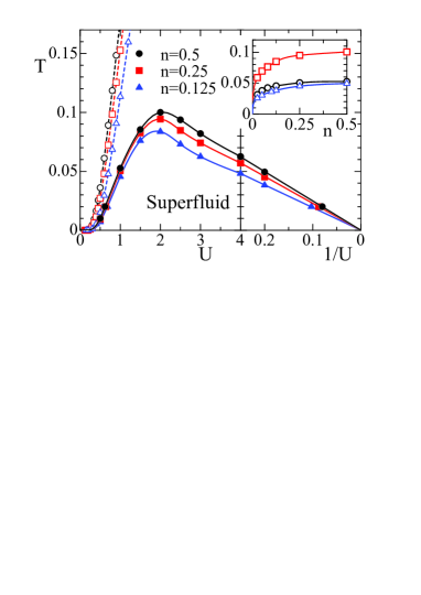
Figure 5: Phase diagrams for the attractive Hubbard model. Circles, squares, and triangles indicate the phase boundaries in the systems with $n=0.5,0.25$ and $0.125$. Solid (open) symbols are the results obtained by DMFT with CTQMC (the BCS theory). Lines are guides to eyes. Inset shows that the critical temperature as a function of the particle density. Open circles, squares, and triangles are the results for $U=1,2$ and $5$.

In the weak coupling region, the BCS-type superfluid state is realized. On the other hand, the BEC-type superfluid state is realized in the strong coupling region, where the phase boundary scales with the inverse of the interaction, as discussed above. The critical temperature reaches its maximum value in all cases $n=0.5,0.25$ and $0.125$ in the intermediate region $(U\sim 2)$, where the BCS-BEC crossover occurs. We also find that a decrease of the particle density monotonically shifts the phase boundary. The inset of Fig. 5 shows the particle density dependence of the critical temperature in systems with $U=1,2$ and $5$. It is found that the critical temperature is slightly decreased away from half filling. When the particle density approaches the dilute limit $(n\rightarrow 0)$, the critical temperature rapidly decreases, as $T_{c}\sim n^{\alpha}$, where $\alpha=0.2\sim 0.3$.

In this section, we have discussed how the superfluid state is realized at low temperatures and determined the phase diagram of the attractive Hubbard model. In the following section, we focus on the dilute system to examine dynamical properties in the BCS-BEC crossover region. We then clarify how the gap structure appears in the density of states.

IV Low-temperature properties near the BCS-BEC crossover

In the section, we study low temperature properties in the intermediate coupling region, where the BCS-BEC crossover occurs. It is known that in the dense system, the BCS-BEC crossover occurs at an interaction which is slightly smaller than the value corresponding to the maximum $T_{c}$ Toschi and no pseudogap appears near the phase boundary KogaQMC1 . On the other hand, it has been reported that a pseudogap always appears at the critical temperature in the Fermi gas system Watanabe . Therefore, it is necessary to clarify how the pseudogap behavior is realized in the dilute system. To clarify this, we focus on the attractive Hubbard model with a low particle density ($n=0.125$) and compute spectral functions in the BCS-BEC crossover region.

We note that the gap structure appears even in the normal state if the preformed pairs are stabilized by the large attractive interaction. This means that it is not directly related to the realization of the superfluid state, but rather to the crossover between the metallic and insulating state, which occurs in the normal phase. To make this clear, we first examine the interaction dependence of dynamical properties at the high temperature $T=0.087$. Figure 6 shows the density of states for the system with $n=0.125$.

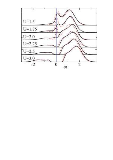
Figure 6: Solid lines indicate the density of states at $T=0.087$ in the system with $n=0.125$. Dashed lines indicate the results at $T=0.02$ in a system which is restricted to be paramagnetic.

We clearly find double peaks in the case $U=1.5$, where the metallic state is realized. A remarkable point is that a large density of states appears around the Fermi level. This is reminiscent of heavy fermion behavior in the repulsive Hubbard model, where a quasi-particle peak develops in the metallic state close to the Mott transition. In the attractive case, if the ground state is restricted to be paramagnetic, a pairing transition occurs between the metallic and insulating states at any filling Capone . The results in the paramagnetic state at a lower temperature $(T=0.02)$ are shown as the dashed lines in Fig. 6. It is found that the sharp quasi-particle peak grows in the region $U\lesssim 2$. Therefore, we conclude that the large density of states near the Fermi level, which appears above the critical temperature at $U=1.5$, results from particle correlations. We wish to note that this behavior is characteristic of the lattice model, in contrast to the interacting Fermi gas system where a gap behavior appears at the critical temperature Watanabe .

Further increase in the attractive interaction leads to the crossover from the heavy metallic state to the insulating state. It is found that the quasi-particle peak collapses and a dip structure appears instead around the maximum $T_{c}$ value $(U\sim 2.0)$. Its width continuously grows with increasing interaction, as shown in Fig. 6. Thus, strong pairing correlations stabilize the gap structure in the vicinity of the Fermi level.

In the intermediate coupling region the crossover between the metallic and insulating states occurs, which is associated with the pairing transition in the normal state, as discussed above. It is known that at zero temperature, this transition point is shifted away from half filling, e.g. $U_{c}\sim 3.0,2.4$ and 1.12 in the cases with $n=0.5,0.25$ and $0_{+}$ Capone . Therefore, we can say that the low energy properties around the critical temperature depend on the particle density as well as the interaction strength. This should have important implications for the observation of the pseudogap behavior in fermionic optical lattices, where these parameters can be controlled experimentally. Namely, in the BCS-BEC crossover region, heavy fermion behavior appears in the dense system KogaQMC1 , while a dip structure (pseudogap behavior) is found in the dilute system.

Let us consider the temperature dependence in the dilute system in the BCS-BEC crossover region. We calculated the pair potential, double occupancy, internal energy, and the specific heat, as shown in Fig. 7.

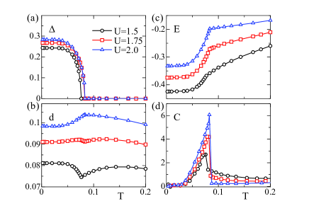
Figure 7: The pair potential (a), the double occupancy (b), the internal energy (c), and the specific heat (d) as a function of temperature around the BCS-BEC crossover.

At the critical temperature, the pair potential is induced, and a cusp singularity appears in the curves of the double occupancy and the internal energy. A jump singularity appears in the curve of the specific heat, and its height increases with increase of the interaction. We note that the cusp singularity in the double occupancy vanishes at a certain interaction $U^{*}(\sim 1.75)$, i.e. $\Delta d/\Delta T|_{T=T_{C}+\delta}=\Delta d/\Delta T|_{T=T_{C}-\delta}$. This is due to the crossover between the heavy metallic state and the insulating state. When the temperature is decreased in the case $U<U^{*}$, the double occupancy reaches a maximum at a certain temperature $T_{max}$ and is decreased as temperature is lowered to the critical temperature. This suggests the formation of the heavy fermion state in the region with $T_{c}<T<T_{max}$. In fact, we find an enhancement of the quasi-particle peak in Fig. 8 (a).

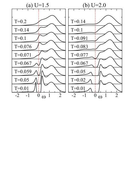
Figure 8: Density of states in the dilute system ($n=0.125$) with $U=1.5$ (a) and $2.0$ (b), where $T_{c}\sim 0.076$ and $0.083$, respectively.

On the other hand, when $U>U^{*}$, the attractive interaction stabilizes preformed pairs at high temperatures and thereby the decrease in the temperature simply increases the double occupancy. Thus the dip structure in the density of states is stabilized above the critical temperature, as shown in Fig. 8 (b).

Below the critical temperature, the static quantities change gradually, as shown in Fig. 7. When $U=1.5$, the decrease of the temperature increases the pair potential, where the heavy quasi-particle peak collapses and the superfluid gap opens around the Fermi level, as shown in Fig. 8 (a). On the other hand, when $U=2.0$, the dip structure found at the critical temperature smoothly evolves into the gap structure at low temperatures. This behavior is also observed in the system with a lower particle density $n=0.025$ at the temperature $T/T_{c}>0.17$. Therefore, we can say that the region with a dip structure at high temperatures is adiabatically connected to that with the superfluid gap at low temperatures. This is in contrast to the results for the three-dimensional Fermi gas system Watanabe . In the gas system, decreasing the temperature around the BCS-BEC crossover smears out the pseudogap structure, and the superfluid gap develops below a certain temperature. This may suggest that $k$-dependent correlations plays a crucial role in realizing these dynamical properties. This topic is beyond the scope of our paper, but it is important to clarify how two kinds of gap structures appear in a low dimensional optical lattice system, by taking into account spatial correlations as well as dynamical correlations.

V Summary

We have investigated the attractive Hubbard model in infinite spatial dimensions by combining dynamical mean-field theory with a strong-coupling continuous-time quantum Monte Carlo method. By calculating the superfluid order parameter and the double occupancy, we have systematically studied the stability of the superfluid state and determined the phase diagram of the system. By computing the density of states, we have found that the gap structure is strongly affected by the interaction strength and the particle density, which is associated with the pairing transition in the normal state. Namely, around the BCS-BEC crossover, a dip structure appears in the dilute system while heavy fermion behavior is found in the dense system. We have also examined the dynamical properties in the superfluid state and have clarified that the dip structure above the critical temperature continuously evolves into the superfluid gap with decreasing temperature.

In this paper, we have considered the dynamical properties characteristic of the infinite-dimensional lattice model, which are qualitatively different from those in the Fermi gas system. It is an interesting problem to clarify how the low energy properties are changed by adding the lattice potential to the Fermi gas system, which is now under consideration.

Appendix

In this study, we have used the strong-coupling version of the CTQMC method to solve the effective Anderson impurity model CTQMC . This method is based on a stochastic sampling of an expansion of the partition function in powers of the impurity-bath hybridization. A given Monte Carlo configuration can be represented by a collection of segments $\{\tau_{i\sigma}^{\prime},\tau_{i\sigma}\}$, where $\tau_{i\sigma}^{\prime}(\tau_{i\sigma})$ is the starting (end) time for the $i$-th segment with spin $\sigma$. These segments represent time intervals in which an electron of spin $\sigma$ resides on the impurity. The Monte Carlo simulation proceeds via local updates, such as insertion/removal of a segment or empty space between segments (called anti-segment), or shifts of segment end-points.

Here, we discuss updates which improve the sampling efficiency in the strong-coupling region. For $|U|\gtrsim 3$, the large energy cost for inserting or removing (anti-) segments leads to a high rejection rate for proposed insertion/removal updates. In fact, the local (impurity) contribution to the Monte Carlo weight is given by

$$w_{loc}=\exp\left[-E_{f}\sum_{\sigma}l_{\sigma}+Ul_{overlap}\right],$$ (9)

where $E_{f}$ is the energy level at the impurity site and $l_{\sigma}$ and $l_{overlap}$ are the total lengths of $\sigma$ segments, and the overlap between up and down segments. Thus, in the strong-coupling regime, at low temperature, the acceptance probability for a generic update will be exponentially suppressed. One possibility is to take this exponential dependence into account on the level of the proposal probabilities. Another possibility to overcome this bottleneck is to consider updates which change the configuration for both spins simultaneously. When both spins are flipped between occupied and unoccupied states in a certain time interval, the energy change on the impurity site is not so large. In particular, the corresponding energy change is zero at half filling $(E_{f}=U/2)$.

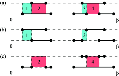
Figure 9: Efficient updates in the strong-coupling regime. The two imaginary time intervals correspond to spin up and down. Bold lines represent segments, i.e. a time interval, in which an electron resides on the impurity. (a) The shaded regions indicate examples of time intervals for which an improved updated will be proposed. (b) Resulting configuration if the update for time intervals 1 and 3 is accepted. These updates correspond to two shifts of segment end-points. (c) Resulting configuration if the update for intervals 2 and 4 is accepted. Here, the update corresponds to two insertions/removals of a segment/antisegment.

We discuss here explicitly one of the simplest of these updates, which is schmatically shown in Fig. 9. We first choose a random time interval, defined by a pair of neighboring creation/annihilation operators $\{\tau_{i\sigma},\tau_{i\sigma}^{\prime}\}$. Note that the spin and type (creator/annihilator) is arbitrary, so the time interval need not correspond to any segment. The proposal probability is given by $p^{prop}=(2N)^{-1}$ where $N$ is the total number of segments. The update consists of flipping both spins in the time interval. Note that this process is composed of two standard updates, i.e. two insertions/removals of a segment/antisegment, or two shift updates. Therefore, it is easy to add these updates to an existing CTQMC code. The above updates were found to improve the efficiency of Monte Carlo simulations in the strong coupling regime.

References

- (1) M. H. Anderson, J. R. Ensher, M. R. Matthews, C. E. Wieman, and E. A. Cornell, Science 269, 198 (1995).
- (2) C. A. Regal, M. Greiner, and D. S. Jin, Phys. Rev. Lett. 92, 040403 (2004).
- (3) S. Jochim,M. Bartenstein, A. Altmeyer, G. Hendl, S. Riedl, C. Chin, J. Hecker Denschlag, and R. Grimm, Science 302, 2101 (2003).
- (4) M. W. Zwierlein,C. A. Stan, C. H. Schunck, S. M. F. Raupach, S. Gupta, Z. Hadzibabic, and W. Ketterle, Phys. Rev. Lett. 91, 250401 (2003).
- (5) T. Bourdel,L. Khaykovich, J. Cubizolles, J. Zhang, F. Chevy, M. Teichmann, L. Tarruell, S. J. J. M. F. Kokkelmans, and C. Salomon, Phys. Rev. Lett. 93, 050401 (2004).
- (6) J. P. Gaebler, J. T. Stewart, T. E. Drake, D. S. Jin, A. Perali, P. Pieri, and G. C. Strinati, Nat. Phys. 6, 569 (2010).
- (7) Q. Chen and K. Levin, Phys. Rev. Lett. 102, 190402 (2009).
- (8) S. Tsuchiya, R. Watanabe, and Y. Ohashi, Phys. Rev. A 80, 033613 (2009).
- (9) C. C. Chien, H. Guo, Y. He, and K. Levin, Phys. Rev. A 81, 023622 (2010).
- (10) S. Q. Su, D. E. Sheehy, J. Moreno, and M. Jarrell, Phys. Rev. A 81, 051604 (2010).
- (11) P. Pieri, L. Pisani, and G. C. Strinati, Phys. Rev. B 70, 094508 (2004).
- (12) R. Watanabe, S. Tsuchiya, and Y. Ohashi, Phys. Rev. A 82, 043630 (2010).
- (13) W. Metzner and D. Vollhardt, Phys. Rev. Lett. 62, 324 (1989).
- (14) E. Müller-Hartmann, Z. Phys. B 74, 507 (1989).
- (15) A. Georges, G. Kotliar, W. Krauth and M. J. Rozenberg, Rev. Mod. Phys. 68, 13 (1996).
- (16) T. Pruschke, M. Jarrell, and J. K. Freericks, Adv. Phys. 44, 187 (1995).
- (17) E. Gull, A. J. Millis, A. N. Rubtsov, A. I. Lichtenstein, M. Troyer, and P. Werner, Rev. Mod. Phys. 83, 349 (2011).
- (18) E. H. Lieb and F. Y. Wu, Phys. Rev. Lett. 20, 1445 (1968).
- (19) H. Shiba, Prog. Theor. Phys. 48, 2171 (1972).
- (20) M. Machida, S. Yamada, Y. Ohashi, and H. Matsumoto, Phys. Rev. A 74, 053621 (2006).
- (21) F. Karim Pour, M. Rigol, S. Wessel, and A. Muramatsu, Phys. Rev. B 75, 161104 (2007).
- (22) G. Xianlong, M. Rizzi, M. Polini, R. Fazio, M. P. Tosi, V. L. Campo Jr., and K. Capelle, Phys. Rev. Lett. 98, 030404 (2007).
- (23) Y. Fujihara, A. Koga, and N. Kawakami, Phys. Rev. A 79, 013610 (2009).
- (24) A. Moreo and D.J. Scalapino, Phys. Rev. Lett. 66, 946 (1991).
- (25) T. Paiva, R. R. dos Santos, R. T. Scalettar, and P. J. H. Denteneer, Phys. Rev. B 69, 184501 (2004).
- (26) A. Koga, T. Higashiyama, K. Inaba, S. Suga, and N. Kawakami, J. Phys. Soc. Jpn. 77, 073602 (2008); Phys. Rev. A 79, 013607 (2009).
- (27) J. K. Freericks, M. Jarrell and D. J. Scalapino, Phys. Rev. B 48, 6302 (1993).
- (28) Y. Y. Suzuki, S. Saito, and S. Kurihara, Prog. Theor. Phys. 102, 953 (1999).
- (29) M. Keller, W. Metzner, and U. Schollwöck, Phys. Rev. Lett. 86, 4612 (2001).
- (30) M. Capone, C. Castellani, and M. Grilli, Phys. Rev. Lett. 88, 126403 (2002).
- (31) A. Garg, H. R. Krishnamurthy, and M. Randeria, Phys. Rev. B 72, 024517 (2005).
- (32) A. Toschi, M. Capone, and C. Castellani, Phys. Rev. B 72, 235118 (2005); A. Toschi, P. Barone, M. Capone, and C. Castellani, New J. Phys. 7, 7 (2005).
- (33) J. Bauer, A. C. Hewson, and N. Dupuis, Phys. Rev. B 79, 214518 (2009); J. Bauer and A. C. Hewson, Europhys. Lett. 85, 27001 (2009).
- (34) A. Privitera, M. Capone, and C. Castellani, Phys. Rev. B 81, 014523 (2010).
- (35) A. Koga and P. Werner, J. Phys. Soc. Jpn. 79, 064401 (2010).
- (36) A. Georges, G. Kotliar, and W. Krauth, Z. Phys. B 92, 313 (1993).
- (37) M. Caffarel and W. Krauth, Phys. Rev. Lett. 72, 1545 (1994).
- (38) H. R. Krishna-murthy, J. W. Wilkins, and K. G. Wilson, Phys. Rev. B 21, 1003 (1980).
- (39) R. Bulla, T. Costi, and Th. Pruschke, Rev. Mod. Phys. 80, 395 (2008).
- (40) O. Sakai and Y. Kuramoto, Solid State Comm. 89, 307 (1994).
- (41) E. Gull, P. Werner, O. Parcollet and M. Troyer, Europhys. Lett. 82, 57003 (2008).
- (42) P. Werner, A. Comanac, L. de’Medici, M. Troyer, and A. J. Millis, Phys. Rev. Lett. 97, 076405 (2006); P. Werner and A. J. Millis, Phys. Rev. B 75, 085108 (2007);
- (43) S. F. Gull, in Maximum Entropy and Bayesian Methods in Science and Engineering, ed. G. J. Erickson and C. R. Smith (Kluwer Academic, Dordrecht, 1988) p. 53; J. Skilling(Kluwer Academic, Dordrecht, 1989) p. 45; S. F. Gull, ibid. p. 53.
- (44) R. N. Silver, D. S. Sivia and J. E. Gubernatis, Phys. Rev. B 41, 2380 (1990); J. E. Gubernatis, M. Jarrell, R. N. Silver and D. S. Sivia, Phys. Rev. B 44, 6011 (1991).
- (45) W. F. Press, S. A. Teukolsky, W. T. Vetterling and B. R. Flannery, Numerical Recipes (Cambridge University Press, Cambridge, 1992) p. 809.
- (46) A. F. Albuquerque, F. Alet, P. Corboz, P. Dayal, A. Feiguin, S. Fuchs, L. Gamper, E. Gull, S. Gurtler, A. Honecker, R. Igarashi, M. Korner, A. Kozhevnikov, A. Lauchli, S. R. Manmana, M. Matsumoto, I. P. McCulloch, F. Michel, R. M. Noack, G. Paw.owski, L. Pollet, T. Pruschke, U. Schollwock, S. Todo, S. Trebst, M. Troyer, P. Werner, S. Wessel, J. Magn. Magn. Mater. 310, 1187 (2007).