Radiation-Hydrodynamic Models of the evolving Circumstellar Medium around Massive Stars

Abstract

We study the evolution of the interstellar and circumstellar media around massive stars ($M\geqslant 40M_{\odot}$) from the main sequence through to the Wolf-Rayet stage by means of radiation-hydrodynamic simulations. We use publicly available stellar evolution models to investigate the different possible structures that can form in the stellar wind bubbles around Wolf-Rayet stars. We find significant differences between models with and without stellar rotation, and between models from different authors. More specifically, we find that the main ingredients in the formation of structures in the Wolf-Rayet wind bubbles are the duration of the Red Supergiant (or Luminous Blue Variable) phase, the amount of mass lost, and the wind velocity during this phase, in agreement with previous authors. Thermal conduction is also included in our models. We find that main-sequence bubbles with thermal conduction are slightly smaller, due to extra cooling which reduces the pressure in the hot, shocked bubble, but that thermal conduction does not appear to significantly influence the formation of structures in post-main-sequence bubbles. Finally, we study the predicted X-ray emission from the models and compare our results with observations of the Wolf-Rayet bubbles S 308, NGC 6888, and RCW 58. We find that bubbles composed primarily of clumps have reduced X-ray luminosity and very soft spectra, while bubbles with shells correspond more closely to observations.

1 Introduction

Massive stars ($M\geqslant 30M_{\odot}$) affect the interstellar (ISM) and their circumstellar (CSM) media due to the combined result of the action of their strong stellar winds and ionizing photons. At early times, massive stars photoionize the surrounding interstellar medium, forming an H II region of $10^{4}$ K gas around themselves, which then begins to expand. The stellar wind from the main-sequence (MS) phase interacts with this photoionized region, producing a hot, tenuous bubble of shocked stellar wind material and a shell of swept-up photoionized gas (Dyson & Williams, 1997). By the end of the main-sequence phase, the massive star will be surrounded by a low density, hot bubble of some $>20$ pc radius for typical densities in star-forming regions, bordered by a thick shell of swept-up neutral material expanding at a few km s^-1 (Cappa et al., 2005; Arthur, 2007). Of course, if the underlying ISM was not homogeneous, or if the star has a substantial velocity relative to the ISM ($>10$ km s^-1), the details will vary but the general picture remains.

When the star evolves off the main sequence, the mass-loss rate increases substantially as the star evolves first towards the red side of the HR diagram and then back to the blue. During this short-lived phase, which can lead to the star becoming a red or yellow supergiant or a luminous blue variable depending on its initial mass, the star can deposit half of its mass as a slow, dense, most-likely neutral wind into its immediate environment. The most intensive phases of stellar mass loss during this period will be episodic and non-spherical ejections of material (Humphreys, 2010). In the final Wolf-Rayet (WR) phase of evolution, this dense circumstellar medium is photoionized by the hot WR star and swept up by the fast WR wind. The circumstellar medium of Wolf-Rayet stars, therefore, contains the history of the most recent, and intense, phases of massive star mass loss.

The slow wind-fast wind interaction has been studied numerically by many authors, who all show that the interaction leads to instabilities (Rayleigh-Taylor and thin shell), which result in the corrugation and eventual break up of the dense shell of swept-up circumstellar material into filaments and clumps. Optical images of the nebulae S 308, NGC 6888 and RCW 58 around the WR stars WR 6, WR 136 and WR 40, respectively, show clear evidence of such a process (Gruendl et al., 2000).

In particular, García-Segura et al. (1996a, b) were the first to study in detail the purely hydrodynamical evolution of WR bubbles and the instabilities which lead to the formation of clumps and filaments. They took into account the evolution of the stellar wind properties from the main sequence through the WR stage for a $35M_{\odot}$ and a $60M_{\odot}$ star as input to their models. Because the winds in the main-sequence and red supergiant stages are comparatively steady, these stages were studied in one-dimensional spherical symmetry, but the formation of instabilities in the slow wind-fast wind interaction at the onset of the WR stage was studied in 2D axisymmetric spherical coordinates. Freyer et al. (2003, 2006) studied the interaction of massive stars ($35M_{\odot}$ and $60M_{\odot}$) with their environment with particular regard to their effect on the energy balance of the interstellar medium. These simulations were performed in two-dimensional cylindrical symmetry from the beginning of the main sequence stage and included the radiative transfer of hydrogen-ionizing radiation. In this way, Freyer et al. (2003, 2006) were able to study the evolution of the H II region around the stellar wind bubble as well as the wind-wind interactions. The stellar wind parameters in this work were the same as those used by García-Segura et al. (1996a, b).

More recent work has related features in supernova and gamma-ray burst (GRB) afterglow absorption spectra to structures in the circumstellar medium around the progenitor stars, where the progenitor of the GRB event is a WR star and the structures are formed during the interaction of the WR wind with the dense, slow wind of the previous evolutionary stage (Ramirez-Ruiz et al., 2005; van Marle et al., 2005; Eldridge et al., 2006; van Marle et al., 2007). Dwarkadas (2007) and Dwarkadas et al. (2010) explored the interaction of the shock wave from the final supernova explosion of the star with the evolved circumstellar medium and compared the simulated X-ray emission with observations of very young supernova remnants.

The evolving circumstellar media around B stars, which do not undergo a WR stage, was modeled by Chita et al. (2007, 2008) where the anisotropy of the stellar winds due to fast stellar rotation was taken into account, producing distinctive hourglass-shaped structures. van Marle et al. (2008) also investigated the effect of rapid rotation on the evolution of a low metallicity $20M_{\odot}$ star, the resultant non-spherical density profiles in the CSM, and the consequences for the GRB afterglow spectra.

In this paper, we are particularly interested in the circumstellar media around Wolf-Rayet stars. Many of the $>200$ known Galactic Wolf-Rayet stars are surrounded by nebulae, visible in optical images. Of these, spectroscopy identifies only 10 as wind-blown bubbles (Chu, 1982; Esteban et al., 1992), of which only 2 have been detected in X-rays. We expect X-rays to arise from the hot, shocked WR wind during the interaction with the ejected slow wind material. The nebula S 308 around WR 6 was detected in soft X-rays by ROSAT (Wrigge, 1999) and XMM Newton (Chu et al., 2003), while NGC 6888 around WR 136 was observed by ROSAT, ASCA, and SUZAKU (Bochkarev, 1988; Wrigge et al., 1994, 1998; Wrigge & Wendker, 2002; Wrigge et al., 2005; Zhekov & Park, 2011). Both WR bubbles show limb-brightened X-ray morphologies and spectra dominated by gas at $T\sim$ 10⁶ K, with the X-ray emission interior to the optical [O III] emision. This X-ray emission is very soft and will be strongly affected by absorption due to neutral hydrogen along the line of sight. S 308 and NGC 6888 are two of the closer WR bubbles (about 1.5 kpc distant) and the greater distance to RCW 58 (about 3 kpc) could explain why it has not been detected in X-rays.

The observed X-ray emission from wind-blown bubbles has proved difficult to model successfully. There are two main schools of thought: on the one hand, if we take a simple hot, wind-blown bubble, such as that described in Dyson & Williams (1997), the temperature of the hot gas is determined by the stellar wind velocity, $kT=3\mu m_{\mathrm{H}}V_{\mathrm{w}}^{2}/16$, where $\mu\sim 0.5$ is the mean particle mass for fully ionized gas. A typical Wolf-Rayet wind velocity is $\sim 1500$ km s^-1, which implies temperatures of $T>3\times 10^{7}$ K in the hot gas. The densities in the hot bubble are very low $n<0.01$ cm^-3, and so this model would predict low luminosity, hard X-rays. On the other hand, there is the oft-used Weaver et al. (1977) model, which assumes thermal conduction between the hot bubble and the “cold” ($10^{4}$ K), swept-up shell. Thermal evaporation of dense, cold material into the hot bubble raises the density and lowers the temperature here. This model predicts high luminosity, soft X-ray emission. Both of these models are one-dimensional (i.e., radial) in concept and do not take into account the break-up of the shell due to instabilities nor the shock-clump interactions which result. The main argument against thermal conduction is that even a weak magnetic field would restrict the movement of the thermal electrons. Diffuse X-ray observations of young star clusters (Dunne et al., 2003; Townsley et al., 2003; Güdel et al., 2008), planetary nebulae (Chu et al., 2003; Guerrero, 2006; Kastner, 2007), as well as the wind-blown bubbles S 308 and NGC 6888 suggest that neither model is entirely applicable, since the observations indicate that the hot gas has a temperature $10^{6}<T<10^{7}$ K but the luminosities are far lower than those predicted by the Weaver et al. (1977) model.

In this paper, we investigate the possible structures that can form around Wolf-Rayet stars by means of radiation-hydrodynamical simulations taking into account the full time evolution of the stellar wind mass-loss rate, terminal velocity and stellar ionizing photon rate, as studied by previous authors. In addition, we include a time-dependent treatment of thermal conduction in our models, which has not been done before. We compare results obtained from three sets of stellar evolution models (Meynet & Maeder, 2003; Eldridge et al., 2006) for stars with masses between $40M_{\odot}$ and $60M_{\odot}$, which include a set of models that take into account stellar rotation. By calculating the chemical abundances expected in the circumstellar nebulae in the post-main-sequence stages of these stellar evolution models, we can make comparisons with optical observations. We also calculate the expected X-ray emission from our numerical simulations under the assumption of collisional ionization equilibrium and compare our results to the wind-blown bubbles S 308, NGC 6888 and RCW 58. By analyzing the structures formed in the circumstellar media of our simulations, the chemical abundance history of the CSM and the time evolution of the X-ray luminosites, we can connect observations to possible mass-loss histories, and hence discriminate between different stellar evolution models.

In § 2 we describe the numerical method including the treatment of thermal conduction, and in § 3 we show the main characteristics of the stellar evolution models. Section § 4 presents our one-dimensional and two-dimensional results and in § 5 we describe our numerical treatment for the simulated luminosity and synthetic spectra, and we make comparisons with both optical and X-ray observations. Section § 6 discusses our results and the effect that differences in the stellar evolution models make to the structures and observational properties of these objects. Finally, § 7 summarizes and concludes our findings.

2 Numerical Method

In this section we provide a general description of the numerical scheme, highlighting new features such as thermal conduction. Full details of the radiation-hydrodynamics scheme are published in the cited references and we describe the main features in Appendix A.

2.1 General description of the numerical scheme

Our simulations are carried out in one and two dimensions. First, the time-dependent, spherically symmetric system of radiation-hydrodynamic equations is solved for the main-sequence and RSG phases, during which the stellar winds are reasonably steady and instabilities are relatively unimportant. Then, the 1D results are remapped to a two-dimensional, cylindrically symmetric $(r,z)$ grid, to continue the evolution of the circumstellar medium through the WR stage, where the density gradients and wind-wind interactions lead to instabilities, which severely disrupt the circumstellar medium.

The 1D spherically symmetric Eulerian hydrodynamic conservation equations are solved using a second order, finite volume Godunov-type scheme with outflow-only boundary conditions at the outer boundary. In 2D, the cylindrically symmetric hydrodynamic conservation equations are solved using a hybrid scheme, in which alternate time steps are calculated by a Godunov method and the van Leer flux-vector splitting method (van Leer, 1982). This reduces numerical artefacts, which can be produced in Godunov-type schemes when slow shocks are propagating parallel to one of the grid directions. The boundary conditions in the 2D scheme are those of no flux through the axis of symmetry and outflow-only conditions at the outer radial and $z$ boundaries.

The 1D simulations start on a grid of 1000 cells with a physical size of 5 pc, which is large enough to contain the initial Strömgren sphere. We use an expanding grid to avoid large computational domains at the beginning of the simulation: when the outer shock nears the edge of the grid, more (uniform ambient medium) cells are added. Each 1D calculation has the same physical resolution (grid cell size $dr=0.002$ pc). By the end of the RSG stage, the stellar wind bubble, H II region and swept-up neutral shell extend up to 30 pc, meaning that the corresponding grids have of order 6000 cells. The full evolution of the CSM around the massive stars is followed in 1D from the beginning of the main-sequence stage through to the WR stage. However, once the star enters the WR stage, 1D is not adequate to capture the full richness of the structures formed during the wind-wind interactions and so we remap the results onto a 2D grid to continue the calculation in cilindrical $r-z$ coordinates.

The majority of the 2D simulations are carried out on a fixed grid of 500 radial by 1000 $z$-direction cells with a corresponding physical size of $10\times 20$ pc² (i.e, cell size $dr\times dz=0.02$ pc$\times 0.02$ pc). This size is chosen because the wind-wind interaction takes place within this distance for almost all models, and the radius of observed WR bubbles is $R\leqslant 10$ pc (Gruendl et al., 2000). One model is run on a slightly larger grid ($750\times 1500$ cells) because the main wind-wind interaction occurs further from the star, but the spatial resolution is the same.

The transfer of the ionizing radiation is carried out by the method of short characteristics (Raga et al., 1999) adapted for spherical and cylindrical symmetry. We consider only a single point source for the ionizing radiation (the star), which is positioned on the symmetry axis. The hydrodynamics and radiative transfer are coupled through the energy equation, where the source term depends on the photoionization heating and the radiative cooling rate, and through advection equations for the ions and neutrals. The ionization balance equation takes into account both photoionization and collisional ionization together with recombination. This basic code has been extensively tested and applied to the evolution of H II regions in density gradients (Henney et al., 2005; Arthur & Hoare, 2006).

The radiative cooling function takes into account both cooling in collisionally ionized gas (in the hot shocked wind bubble) and in the photoionized gas in the H II region where collisional ionization of hydrogen is not an important contribution to the cooling rate. Cooling rates are generated using the Cloudy photoionization code (Ferland et al., 1998) for appropriate stellar parameters and used to generate a look-up table. The cooling rates extend down to temperatures of 100 K but photoionization heating ensures that the H II region has a temperature of $\sim 10^{4}$ K.

The stellar wind is input to the grid through the Chevalier & Clegg (1985) thermal wind model, as a volume-distributed source of mass and energy. This avoids the problem of reverse shocks that can occur when there is a decrease in the ram pressure of a stellar wind input in the form of a region of high-density, high-velocity flow near the origin. The volume of the stellar wind injection region is chosen to be sufficiently small so that the stellar wind always reaches its terminal velocity and shocks outside the source region, but sufficiently large so as to be a reasonable geometrical representation of a sphere on a cylindrical grid (in the case of the 2D numerical simulations).

The variation of the stellar mass-loss rate with time is taken from publicly available stellar evolution models (Meynet & Maeder, 2003; Eldridge et al., 2006). The stellar wind velocities are calculated using the tabulated stellar parameters (mass, radius, effective temperature and surface abundances) and the ionizing photon rates are obtained from the appropriate stellar atmosphere models distributed with the Starburst 99 code (Leitherer et al., 1999). All of this information is stored in tables and interpolated as needed using the elapsed simulation time.

2.2 Thermal Conduction

We also run a set of models that includes the effects of electron thermal conduction to assess the importance of this physical process for the dynamics of stellar wind bubbles and their observable properties such as X-ray emission (Weaver et al., 1977). Thermal conduction is taken to be a diffusion process, with the heat flux, $\vec{q}$, given by

$$\vec{q}=-D\nabla T_{e},$$ (1)

where $D$ is the diffusion coefficient and $T_{e}$ is the electron temperature (Cowie & McKee, 1977). From Spitzer (1962), we have that the electron mean free path can be written as

$$\lambda_{e}=2.625\times 10^{5}T_{e}^{2}/n_{e}/\ln\Lambda,$$ (2)

where $n_{e}$ is the electron number density and $\ln\Lambda$ is the Coulomb Logarithm. For a pure hydrogen plasma this can be approximated by

$$\ln\Lambda=9.452+3/2\ln T_{e}-\frac{1}{2}\ln n_{e}$$ (3)

when $T_{e}\leq 4.2\times 10^{5}$ K and,

$$\ln\Lambda=22.37+\ln T_{e}-\frac{1}{2}\ln n_{e}$$ (4)

when $T_{e}\geq 4.2\times 10^{5}$ K.

From Steffen et al. (2008), the diffusion coefficient $D$ is then given by

$$D=7.04\times 10^{-11}\lambda_{e}n_{e}T_{e}^{1/2},$$ (5)

where the numerical coefficient is the result of evaluating physical constants (Spitzer, 1962). In spherical symmetry, the non-linear diffusion equation is

$$\frac{\partial e}{\partial t}=\rho c_{v}\frac{\partial T_{e}}{\partial t}=\frac{1}{r^{2}}\frac{\partial}{\partial r}\left(r^{2}D\frac{\partial T_{e}}{\partial r}\right),$$ (6)

and we solve this using a Crank-Nicholson-type scheme (Press et al., 1992). Thermal conduction is also included in the 2D simulations by solving the corresponding diffusion equation in cylindrical symmetry. The effect of conduction is included as an update to the internal energy, $e$, once the diffusion equation has been solved for the electron temperature, and we assume equipartition between the electrons and ions.

When the electron temperature $T_{e}$ is high and the electron density $n_{e}$ low, the electron mean free path $\lambda_{e}$ becomes large compared to the size scale of the hot bubble, and the diffusion approximation breaks down. This is the saturated heat flux limit (Cowie & McKee, 1977) that can be described as

$$q_{\mathrm{sat}}=1.72\times 10^{-11}T_{e}^{3/2}n_{e}.$$ (7)

Saturated conduction is treated by limiting the electron mean free path in the following manner

$$\lambda=\min\{0.244\Delta r,2.625\times 10^{5}T_{e}^{2}/n_{e}\ln\Lambda\},$$ (8)

where $\Delta r$ is the local grid spacing and the numerical constant ensures that the conductive heat flux can never exceed the saturation limit (Steffen et al., 2008). This formulation means that the limiting flux can only be reached at the sharp edge of the hot bubble, where $|\Delta T_{e}|\approx T_{e}$. A drawback of this method of limiting the electron mean free path is that it depends explicitly on the numerical resolution $\Delta r$ and so our results will be affected by this. However, since all our 1D results are run at the same numerical resolution, comparisons between simulations are perfectly valid.

The temperature found from solving the diffusion equation for every grid cell is used to update the internal energy of that cell once the hydrodynamic and radiation steps have been completed.

3 Stellar Evolution Models

In this paper we use the publicly available stellar evolution models for initial stellar masses of 40 and $60\,M_{\odot}$ from Meynet & Maeder (2003), hereafter MM2003, and the 40, 45, 50, 55, and $60\,M_{\odot}$ initial mass models from STARS (Eggleton, 1971; Pols et al., 1995; Eldridge & Tout, 2004). Both evolutionary models use the same nuclear reaction rates based on the NACRE database (Angulo et al., 1999), and OPAL opacities (Iglesias & Rogers, 1996). At low temperatures, the opacities come from Alexander & Ferguson (1994) and Ferguson et al. (2005). Differences between the codes such as assumptions, approximations, and solution algorithms, lead to differences in the post-main-sequence evolution of the massive stars.

We consider only the Solar metallicity models, which for MM2003 means $X=0.705$ and $Y=0.275$, while for STARS this is $X=0.7$ and $Y=0.28$ for $Z=0.02$. In addition, MM2003 provide models including stellar rotation, and so we investigate the differences between models with and without rotation. The principal effects of an initial fast stellar rotation are to increase the main-sequence lifetime of the star by about $15$–$25\%$, and also to extend the lifetimes of the stars in the Wolf-Rayet stage (Meynet & Maeder, 2003). Furthermore, the nature of the intense period of post-main-sequence mass loss can change, for example, the $60M_{\odot}$ MM2003 model without rotation undergoes a short-lived period of intense mass loss that can be interpreted as a Luminous Blue Variable (LBV) phase, while the corresponding model with rotation never becomes an LBV. Models from STARS do not include rotation.

We use the MM2003 models with an initial equatorial rotation velocity of 300 km s^-1. This rotation velocity is large enough such that rotation effects on the stellar evolution are important, but not so large that anisotropies in the stellar wind are important in the later stages of stellar evolution. MM2003 find that, for an initial rotation velocity of 300 km s^-1, during the WR stage the ratio of the stellar surface velocity to the break-up velocity is very small for the 40 and 60$M_{\odot}$ stellar models (see their fig. 2) and so we do not expect the stellar winds to become strongly anisotropic during this stage (Ignace et al., 1996). We do not take into account the episodic and non-spherical nature of the wind during the most intense phases of mass loss (Humphreys, 2010).

Figure 1: Mass-loss rate for top panel $40\,M_{\odot}$ and bottom panel $60M_{\odot}$ models. In each panel, solid line — MM2003 no rotation, dashed line – MM2003 with rotation, dotted line — STARS.

Mass loss is very important in the evolution of massive stars. For the mass-loss rates in pre-WR evolution, MM2003 use the theoretical mass-loss rates of Vink et al. (2001), while STARS uses the empirical mass-loss rates from de Jager et al. (1988). In the WR phase, both evolution codes use the mass-loss rates proposed by Nugis & Lamers (2000). In Figure 1 we compare the mass-loss rates of the MM2003 and STARS models. Although the details of the main-sequence mass loss is very similar in each case, there are appreciable differences in the lifetimes of the different post-main-sequence stages and the peak mass-loss rate. The MM2003 model with rotation has a far longer main-sequence lifetime.

Figure 2: Stellar wind velocity for top panel $40\,M_{\odot}$ and bottom panel $60M_{\odot}$ models. In each panel the models are, solid line — MM2003 no rotation, dashed line – MM2003 with rotation, dotted line — STARS.

Our radiation-hydrodynamic simulations take the mass-loss rates as a function of time directly from the stellar evolution models. We also need the stellar wind velocities and ionizing photon rates for our simulations, and these can be calculated using the values of the stellar radius, effective temperature, and surface abundances from the stellar evolution models. The stellar wind velocities for the MM2003 models are calculated as in Kudritzki et al. (1989) for the main sequence phase, then we use 30 km s^-1 for the red/yellow supergiant wind ($T_{\mathrm{eff}}<8\,000$ K) or 200 km s^-1 for the LBV wind ($8\,000<T<25\,000$ K and $\log\dot{M}>-3.9$), as adopted in the Starburst 99 code (Leitherer et al., 1999, and updates). The wind velocities in the WR phase (defined by surface hydrogen mass fraction $X<0.4$ and $T_{\mathrm{eff}}>25\,000$ K) are taken from the tables of Smith et al. (2002). For the STARS models, the wind velocities are listed as part of the stellar evolution tables, using the formulae in Vink et al. (2001) for the pre-Wolf-Rayet phase and those of Nugis & Lamers (2000) for the Wolf-Rayet phase. We corrected the tabulated values by the appropriate constant factors after noting errors in the wind velocities. The resulting wind velocities are lower in the RSG phase, even dropping as low as 5 km s^-1, and are also lower in the WR phase compared to the values we adopt for the MM2003 models. The stellar wind velocities are shown in Figure 2. It is apparent that the WR stellar wind velocities obtained from the Smith et al. (2002) tables are extremely high, particularly in the final stages of stellar evolution. These velocities were taken from the $v_{\infty}$-spectral type calibrations of Prinja et al. (1990), where spectral type is estimated from the stellar effective temperature and surface chemical composition. The WR wind velocities obtained by using the fits of Nugis & Lamers (2000) depend on the escape velocity of the hydrostatic core, the luminosity and the surface abundances, and are generally lower.

The ionizing photon rate was obtained by using appropriate stellar atmosphere models and integrating over the ionizing flux. For both MM2003 and STARS models, we used the stellar atmosphere tables from Starburst 99 (Leitherer et al., 1999), concretely the atmosphere models of Pauldrach et al. (2001) for the main-sequence stage, the stellar library of Lejeune et al. (1997) for the post-main sequence stage, and for the WR stage we use the models of Hillier & Miller (1998), as described by Smith et al. (2002). The resultant ionizing photon rates as a function of time are shown in Figure 3.

Figure 3: Ionizing photon rates for top panel $40\,M_{\odot}$ and bottom panel $60M_{\odot}$ models. In each panel the models are, solid line — MM2003 no rotation, dashed line – MM2003 with rotation, dotted line — STARS.

Figure 4: Evolutionary tracks in the $T_{\mathrm{eff}}$–luminosity plane. Top panel: MM2003 models. Solid lines indicate no stellar rotation, dashed lines indicate models with rotation, for $60M_{\odot}$ (upper) and $40\,M_{\odot}$ (lower) initial masses. Bottom panel: STARS models. Solid line – $40\,M_{\odot}$, dashed line – $50M_{\odot}$, dotted line – $60M_{\odot}$. In each panel, the circle, square and triangle represent the values for WR 6, WR 40 and WR 136 from Hamann et al. (2006), respectively. The region delimited by the thin vertical lines indicates the effective temperature range for which the stars would be considered yellow supergiants (4800 – 7500 K).

In Figure 4 we plot the evolutionary tracks for the $40\,M_{\odot}$ and $60\,M_{\odot}$ MM2003 and STARS models together with data points that represent the properties of the WR stars WR 6, WR 40, and WR 136 from Hamann et al. (2006). These are the central stars of the three WR wind-blown bubbles S 308, RCW 58, and NGC 6888, respectively. The initial masses of these WR stars have been controversial. We can see that the WN4 star WR 6 falls exactly on the evolutionary track of the $40\,M_{\odot}$ no-rotation model from MM2003 but slightly below the corresponding model with rotation, while it lies between the $40$ and $50M_{\odot}$ STARS models. The WN8 star WR 40 seems to fit the $60\,M_{\odot}$ models from MM2003, but apparently would require a much higher mass model from STARS. Finally, the WN6 star WR 136 would indicate an initial mass lower than $40\,M_{\odot}$ in both sets of models. However, there are large uncertainties in the luminosities of these stars due to variability and distance determinations.

4 Results

We present results of our one and two-dimensional simulations. The 1D spherically symmetric simulations are used to follow the formation of the main-sequence stellar wind bubble and H II region and to have a general idea of the evolution of the circumstellar medium once the star has left the main sequence. Two-dimensional, cylindrically symmetric ($r,z$) simulations are used to study the interaction between the fast WR wind and the slow, dense RSG wind, where instabilities are expected to break the swept-up shell into clumps. The starting point for the 2D simulations are the results of the spherically symmetric simulations at the end of the RSG phase, which we remap onto the cylindrical grid.

4.1 1D Results

4.1.1 Main-sequence stage

We start from an initial condition of a cold, uniform, neutral medium with density $n_{0}=100$ cm^-3 and temperature $T=100$ K. The photoionized (H II) region forms first. The photoionized gas is heated to $T\sim 10^{4}$ K and begins to expand into the surrounding medium at $v_{\mathrm{if}}\gtrsim 10$ km s^-1. The conditions at the ionization front require a shock to form in the neutral medium ahead of it, which sweeps up and compresses the neutral gas. Inside the H II region, the highly supersonic stellar wind forms a two-shock structure: an outer shock sweeps up, heats and compresses the photoionized gas, and an inner shock brakes and heats the stellar wind. The two regions have the same pressure but different densities and are separated by a contact discontinuity. The outer shocked region can cool down quickly to the temperature of the H II region due to the high densities in the swept-up material, but its temperature is maintained at $10^{4}$ K by photoionization. The shocked stellar wind, on the other hand, has a very high temperature ($T>10^{7}$ K) and low density and so does not cool efficiently. A hot bubble forms inside the H II region, which is in turn surrounded by a slowly expanding shell of swept-up neutral material. These structures are well known from textbooks (e.g., Dyson & Williams, 1997) and the slow time evolution of the stellar parameters does not cause any noticeable modifications. The evolution of a stellar wind bubble inside an H II region is different to that when ionization is not taken into account (e.g., van Marle et al., 2004). Once the initial Strömgren region has been formed, the pressure in the H II region is much higher than that in the surrounding ISM. Moreover, although to begin with the pressure in the hot, shocked, stellar wind bubble is higher than that in the photoionized gas, pressure equilibrium with the H II is reached after a short time and, thereafter, the pressure across the bubble structure is regulated by both the H II region and the stellar wind together.

To illustrate the main-sequence evolution, in Figure 5 we show the results from a 40$M_{\odot}$ STARS model for simulations with and without thermal conduction after $t=10^{6}$ yrs. The hot, shocked wind bubble, H II region, and neutral shell are cleary identified. The bubble radius in the simulation with thermal conduction is slightly smaller than that without conduction due to increased radiative losses in the hot bubble. These enhanced radiative losses in the hot, stellar wind bubble reduce the pressure here and enable the H II region to expand back towards the star, and the phoionized gas has slightly lower density in the thermal conduction simulations that in those without conduction as a result.

Table 1: Radii and masses of the outer H I shell at the end of MS phase

Mass	Model	$R_{\mathrm{HI}}$	$M_{\mathrm{ism}}$
$M_{\odot}$		pc	$M_{\odot}$
40	MM2003 N	24.6	$2.0\times 10^{5}$
40	MM2003 R	27.5	$2.8\times 10^{5}$
40	STARS	29.0	$3.3\times 10^{5}$
60	MM2003 N	25.6	$2.2\times 10^{5}$
60	MM2003 R	29.4	$3.4\times 10^{5}$
60	STARS	29.4	$3.4\times 10^{5}$

For our particular models, we find that by the end of MS stage, the radius of the region affected by the massive star is 25–30 pc (see Table 1) and the mass of swept-up neutral material is $>10^{5}M_{\odot}$. The exact size of the bubble depends mainly on the length of the main-sequence stage (e.g., models with rotation have longer main sequences than those without) and the stellar wind velocity. Higher stellar wind velocities lead to higher pressures in the shocked wind bubbles and therefore faster expansion speeds (e.g., the STARS models have higher main-sequence stellar wind velocities, see Fig. 2). We remark that bubbles expanding into denser media will, of course, be smaller, since on dimensional grounds the external radius of a stellar wind bubble in an uniform medium of density $n_{o}$ is $R\sim(\dot{M_{W}}V_{w}^{2}/n_{0})^{1/5}t^{3/5}$ where $\dot{M_{W}}$ is the mass-loss rate and $V_{W}$ the stellar wind velocity (see e.g. Dyson & Williams, 1997), while that of an expanding H II region follows $R_{\mathrm{i}}\sim(S_{*}/\alpha_{\mathrm{B}}n_{0}^{2})^{3/7}c_{\mathrm{II}}^{4/7}t^{4/7}$, where $\alpha_{\mathrm{B}}$ and $c_{\mathrm{II}}$ are the recombination coefficient and the sound speed in the ionized gas, respectively, and $S_{*}$ is the stellar ionizing photon rate. Both of these relations depend inversely on the density (Spitzer, 1978).

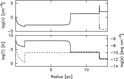
Figure 5: Density and temperature at $10^{6}$ yrs of evolution for the 40$M_{\odot}$ model from STARS. Left-hand panels: model without thermal conduction, right-hand panels: model with thermal conduction. The density plots show total density (solid line) and ionized density (dashed line). The temperature plots also show the internal energy, $e=p/[\gamma-1]$ (dashed line).

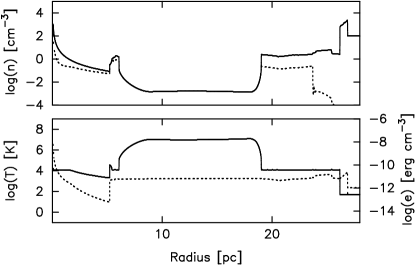
Figure 6: Density and temperature at the end of the RSG phase for the $40\,M_{\odot}$ models. Left-hand panels: MM2003 models, right-hand panels: STARS models. Top row: models without thermal conduction, bottom row: models with thermal conduction. The density plots show total density (solid line) and ionized density (dashed line). The temperature plots also show the internal energy, $e=p/[\gamma-1]$ (dashed line).

Figure 7: Same as Fig. 6 but for the $60\,M_{\odot}$ models.

4.1.2 Post-main-sequence stage

During the RSG phase the star loses a large amount of its mass in a slow, dense wind (see Fig. 1). This wind is subsonic with respect to the hot wind bubble left by the main-sequence stellar wind and so piles up at the bottom of a $r^{-2}$ density gradient into a thin dense shell without forming a two-shock pattern.

In Figure 6 we show the density, temperature and internal energy (i.e. thermal pressure, since $e=p/[\gamma-1]$) as a function of radius at the end of RSG phase for the $40\,M_{\odot}$ models. We compare the results using the MM2003 stellar evolution model (without rotation) with those of STARS. For the simulations without thermal conduction, we see an inner region of RSG wind, which has a $r^{-2}$ density profile and temperature $T<10^{4}$ K, with a high central density and bounded by a dense shell of partially ionized material. For the MM2003 model, this region has a radius of $\sim 6$ pc, while for the STARS model the radius is only $\sim 2$ pc, the shell is much narrower and the densities are higher. This is because the RSG phase is much shorter in the STARS models, even though roughly the same amount of stellar mass is lost as in the MM2003 models. The ram pressure of the RSG wind is less than the thermal pressure of the hot, shocked bubble produced during the main-sequence stage. As a result, there is some back filling as the hot diffuse gas pushes back towards the star. The lack of ionizing photons at this stage (see Fig. 3), and enhanced opacity due to the RSG wind and neutral shell, leads to recombinations in the outer H II region at radius $R\sim 27$ pc. This is most pronounced for the MM2003 model, since the inner absorbing RSG shell contains more neutral atoms than the shell formed in the STARS case. When thermal conduction is included in the simulations, evaporation of cold material from both the RSG shell and the outer H II region enhances the density and thus the cooling rate in the hot shocked wind bubble. In the MM2003 case, this results in a much smaller hot bubble ($\sim 19$ pc as opposed to $\sim 27$ pc in the simulation without conduction). The circumstellar medium in the STARS simulations is less affected by thermal conduction, possibly due to the shorter timescales in the RSG phase.

In Figure 7 we show the corresponding circumstellar structures for the $60\,M_{\odot}$ models at the end of the RSG phase. The MM2003 and STARS results look quite different. This is because the MM2003 model experiences several episodes of enhanced mass loss, whereas the STARS model undergoes a single intense outburst. The ram pressure of the slow wind in the MM2003 case fluctuates and this leads to acoustic waves propagating from the inner edge of the hot bubble outwards. In Figure 7 the waves have yet to reach the outer edge of the bubble, but once they do, they will reflect from the dense neutral shell and pass back through the bubble and reflect backwards and forwards through the hot shocked gas, forming localized heated and compressed regions where oppositely directed waves shock against each other. There is no clearly defined shell of RSG material in the $60\,M_{\odot}$ models, because the duration of the most intense period of mass loss is very short and just before the onset of the WR phase (see Fig. 1), hence the dense material has not had time to move far away from the star before the fast wind starts.

We are particularly interested in the radii of the dense, neutral RSG shells formed in these models. These shells will be impacted and broken up by the fast WR winds and so have important consequences for the observables (X-ray and optical emission) of the WR wind-blown bubbles. The shells are most evident in the $40\,M_{\odot}$ models, reaching radii of $\sim 6$ pc and $\sim 2$ pc for the MM2003 and STARS models, respectively, by the end of the RSG phase. These distances reflect the duration of the RSG stage in each case: $5.6\times 10^{5}$ yrs for the MM2003 model as opposed to $3.1\times 10^{5}$ yrs for the STARS model. Also, the wind velocities in the STARS model are allowed to fall below 30 km s^-1 and in general are lower that those of the MM2003 models (see Fig. 2). We have not presented results for the MM2003 models with stellar rotation because they are qualitatively similar to the results for the other models and result in a dense neutral shell being formed at $\sim 2$ pc, since the RSG phase in this model only lasts $1.0\times 10^{5}$ yrs. We continue the simulations in 1D until the end of the WR phase but we do not show these models because we are interested in the formation of instabilities during the fast wind-slow wind interaction, which do not occur in 1D.

4.2 2D Results

At the end of the RSG phase, we remap our 1D, spherically symmetric distributions of density, momentum and energy onto a 2D axisymmetric grid using a volume-weighted averaging procedure to ensure conservation of these quantities. The 2D grid is, of computational necessity, coarser than the 1D grid, and we also zoom in on the inner $\sim 10$ pc of the simulation, since this is where the hydrodynamic interaction between the fast WR wind and the slow RSG wind will take place. Also, the observed WR bubbles all have radii 10 pc or less. We continue to follow the radiation-hydrodynamic evolution of the circumstellar medium using the stellar wind parameters and the tabulated ionizing photon rate as a function of time shown in Figures. 1, 2, and 3. For all 2D simulations, we present only one quadrant of the calculation, since the other is the same due to symmetry.

4.2.1 $40M_{\odot}$ models

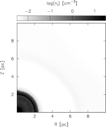
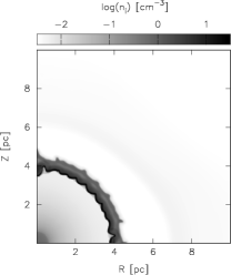
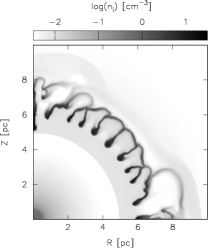
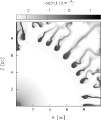
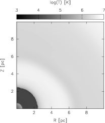
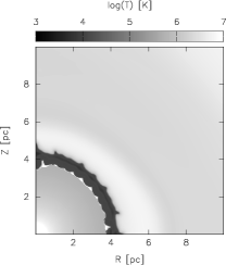
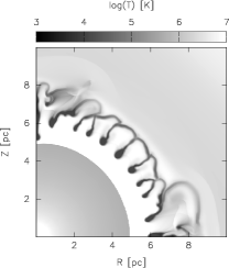
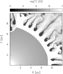
Figure 8: Wind-wind interaction for the $40\,M_{\odot}$ STARS model without thermal conduction. From left to right the evolution times are $39800,65900,86000,$ and $104000$ yrs after the onset of the WR wind. Top panels show ionized number density and bottom panels show temperature, both on logarithmic scale.

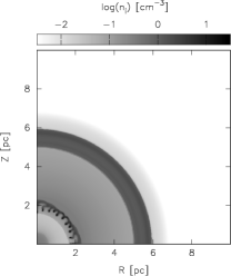
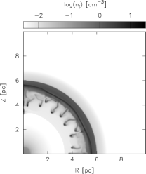
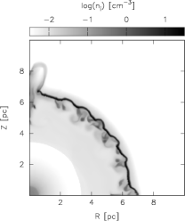
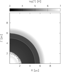
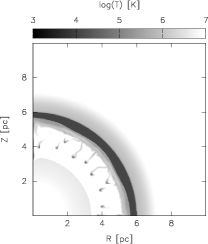
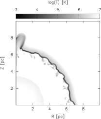
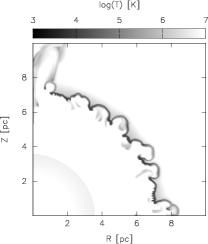
Figure 9: Same as Figure 8 but for the $40\,M_{\odot}$ MM2003 model without stellar rotation and without thermal conduction. From left to right the evolution times are $10600,22600,32650,$ and $36600$ yrs after the onset of the WR wind.

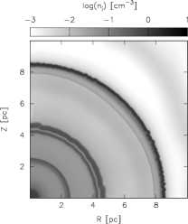
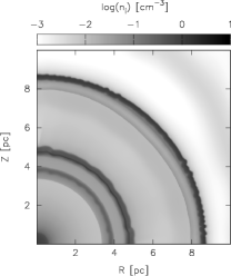
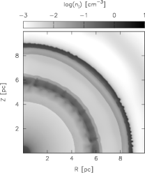
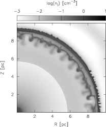
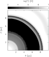
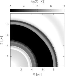
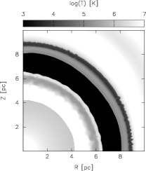
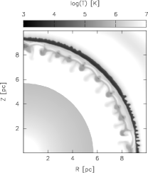
Figure 10: Same as Figure 8 but for the $40\,M_{\odot}$ MM2003 model with stellar rotation without thermal conduction. From left to right the evolution times are $6800,8800,12800,$ and $16900$ yrs after the onset of the WR wind.

In Figure 8 we present grayscale images for the wind-wind interaction for the $40\,M_{\odot}$ STARS model without thermal conduction at four different times corresponding to when the interaction region has reached distances 2, 4, 6, and 8 pc from the central star. These times are, respectively, $39800,65900,86000,$ and $104000$ yrs after the onset of the WR wind. In this figure, we see the disruption of the RSG shell by the fast wind and the formation of clumps. The RSG material consisted initially of a thin, dense shell of partially ionized material located $\sim 2$ pc from the star. The fast WR wind accelerates down the density gradient and slams into the dense shell. The WR wind is shocked and heated by this interaction while the dense shell is shocked and compressed. Vishniac instabilities of the linear thin-shell variety break the shell into dense clumps, which then travel radially outwards (Vishniac, 1983; Vishniac & Ryu, 1989). The clumps have a cometary form, with the dense, cold ($10^{4}$ K photoionized) head pointing towards the central star and tails extending several parsecs radially outwards, showing that the heads are traveling more slowly than the diffuse material that surrounds them. Interactions between clump material and the shocked fast wind create a pattern of multiple interacting shocks, which heat the ablated clump gas to X-ray temperatures. For this particular case the RSG shell breaks up at $\sim 5$ pc (see Fig. 8).

Figure 9 shows the results obtained when the stellar wind parameters come from the MM2003 $40\,M_{\odot}$ model without rotation and without conduction. The wind-wind interaction region is again shown at 2, 4, 6 and 8 pc from the central star, corresponding to $10600,22600,32650,$ and $36600$ yrs after the onset of the WR wind. For this model, the RSG dense wind material, traveling at $\sim 30$ km s^-1, is in the form of a broad shell about 6 pc from the star at the start of the WR stage. The interaction of the WR wind with this shell occurs only a few times $10^{3}$ yrs after the onset of the fast wind. Compared to the STARS model, the MM2003 models experience Rayleigh-Taylor instabilities, which disrupt the accelerating WR shell before it interacts with the main shell of RSG material, forming small clumps at $<2$ pc. The main interaction of the WR shell with the RSG shell occurs at 6 pc and compresses the RSG material into a very thin, dense shell, which then corrugates and starts to break up at around 8 pc due to the linear thin-shell instability.

Figure 10 shows the results from MM2003 model with stellar rotation but without conduction at $6800,8800,12800,$ and $16900$ yrs after the onset of the WR wind. In this model the interaction takes place much further from the star and the shell of RSG material is not so dense, so the interaction does not produce such violent instabilities and the shell remains essentially intact, being swept up and compressed by the fast wind but not suffering the complete disruption seen in the STARS case discussed above. For this model, the intense mass-loss phase has a relatively short duration, $\sim 10^{5}$ yrs, and there are several mass-loss episodes before and after the main ejection event. Rather than a RSG stage, the extremely strong mass loss ($\dot{M}_{\mathrm{w}}\sim 10^{-3.6}M_{\odot}$ yr^-1), together with the fact that the stellar effective temperature is relatively high ($T_{\mathrm{eff}}\sim 10^{4}$ K) for part of this period, indicate a Luminous Blue Variable stage, with stellar wind velocities $V_{\mathrm{w}}>200$ km s^-1. The densest wind material travels quite a large distance from the star before the onset of the WR stage and so the interaction with the fast wind, when it occurs, does not lead to complete breakup of the shell.

We find that thermal conduction has little discernible effect either on the density or the temperature structure of the 2D simulations and the results are essentially the same as those shown in Figures 8, 9 and 10. In Figure 11 we present one set of results including thermal conduction to illustrate this. In this figure we show the results of the $40\,M_{\odot}$ MM2003 simulations (without rotation) at 36600 yrs after the onset of the WR wind. There are slight differences between the two sets of results, but the short timescales of the wind-wind interaction stage compared to cooling timescales in the $10^{6}$ K gas mean that there is no major effect on the hydrodynamics due to thermal conduction during this stage.

We have run further set of STARS simulations to investigate the effects of the radius of the wind injection zone and the grid resolution on the number and distribution of clumps formed during shell disruption. Increasing the grid resolution to 800$\times$1600 cells while maintaining the same number of cells in the wind injection region (radius 30 cells) produced the same results as those presented here. Decreasing the size of the wind injection region (radius 10 cells) did produce fewer clumps but increasing the radius of the wind injection region to 50 cells gave the same results as in Figure 8. The clumps formed in our simulations have diameters between 15 and 50 cells and are photoionized, hence are fully resolved.

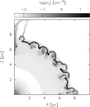
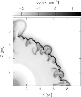
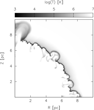
Figure 11: Ionized density (Top panels) and temperature (bottom panels) during the interaction of the fast WR wind with the slow, dense RSG wind for the $40\,M_{\odot}$ MM2003 model without stellar rotation. Left panel: model without thermal conduction Right panel: with thermal conduction. Both numerical results are at $36600$ yrs after the the onset of the WR stage.

4.2.2 $60M_{\odot}$ models

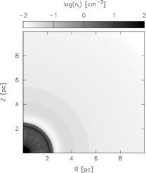
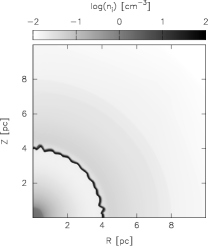
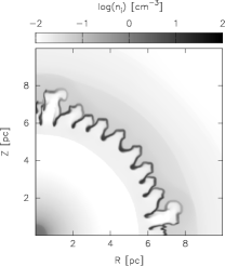
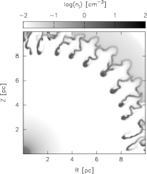
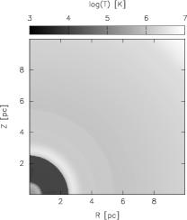
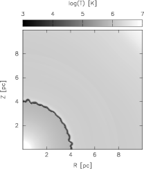
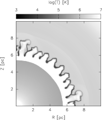
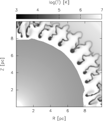
Figure 12: Wind-wind interaction for the $60\,M_{\odot}$ STARS model without thermal conduction. From left to right the evolution times are $27150,43200,57200,$ and $71250$ yrs after the onset of the WR wind.

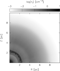
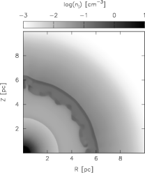
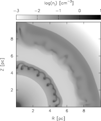
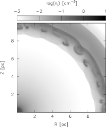
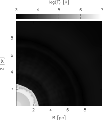
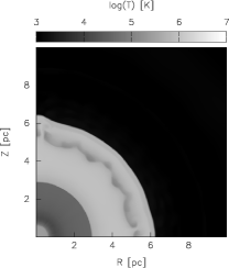
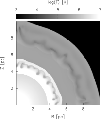
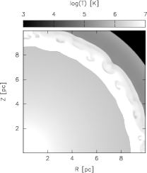
Figure 13: Same as Figure 12 but for the $60\,M_{\odot}$ MM2003 model without stellar rotation and without thermal conduction. From left to right the evolution times are $6800,14800,24800,$ and $30900$ yrs after the onset of the WR wind.

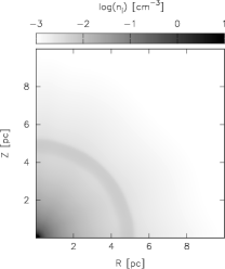
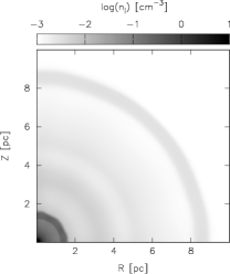
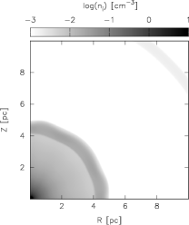
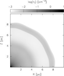
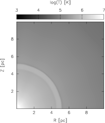
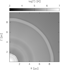
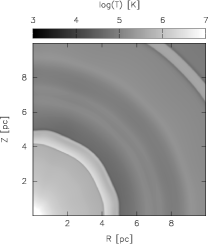
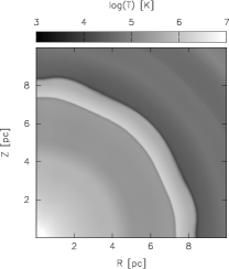
Figure 14: Same as Figure 12 but for the $60\,M_{\odot}$ MM2003 model with stellar rotation and without thermal conduction. From left to right the evolution times are $19450,21450,23450,$ and $25500$ yrs after the onset of the WR wind.

In Figure 12 we show the corresponding results for the $60\,M_{\odot}$ STARS model without conduction. Again, we show the wind-wind interaction at 2, 4, 6, and 8 pc, corresponding to evolution times of $27150,43200,57200,$ and $71250$ yrs after the onset of the WR wind. The dense RSG (or LBV) material is swept up into a thin shell by the fast WR wind. Linear thin-shell instabilities are induced in the swept-up material and break the shell into many cold ($<10^{4}$ K), dense ($>1$ cm^-3) clumps which drift outwards, embedded in the hot, shocked WR wind. The morphologies of the $40\,M_{\odot}$ and $60\,M_{\odot}$ STARS models are very similiar.

For the MM2003 $60\,M_{\odot}$ model without rotation, there are several episodes of enhanced mass loss during the RSG/LBV stage and even in the WR stage there are short-lived outbursts (see Fig. 1). This leads to the formation of successive shells of material traveling with different velocities away from the star shown in Figure 13. The most intense mass-loss episode shown in Figure 1 is followed by a reduction in mass-loss rate and increase in wind velocity (see Fig. 2), which sweeps up, compresses and accelerates the ejected material. This leads to the formation of Rayleigh-Taylor instabilities, which disrupt the shell once it has reached $\sim 10$ pc from the star. The clumpy shell is traveling quite quickly and soon leaves the region of interest ($R<10$ pc). Other, less dense, shells follow, which suffer instabilities but do not contain enough material to form dense, cold clumps. In Figure 13 we show the wind-wind interaction and the formation of different shells and shock patterns as a result of the variability of the mass-loss and wind velocity up to 30,900 yrs after the onset of the WR wind.

For the MM2003 $60\,M_{\odot}$ model with rotation, from Figure 1 we note that there is no period of particularly enhanced mass loss. In this case, therefore, although the RSG is swept up by the faster WR wind, the swept-up material is not particularly dense and does not form a thin, dense shell nor any instabilities or clumps. In Figure 14 we show the density and temperature in the evolving CSM up to the point when the swept-up material has reached a radius of 8 pc from the star, which occurs 25,500 yrs after the onset of the WR stage.

4.3 Comparisons with previous works

Differences between our results and the work of previous authors can be attributed to several factors: the stellar evolution models, the numerical method, and the initial conditions and physics that is included in the numerical simulations. In this section we discuss each of these aspects in turn.

Much of the previous numerical work on the evolving circumstellar media around massive stars has used the same $35\,M_{\odot}$ and $60\,M_{\odot}$ stellar evolution models as García-Segura et al. (1996a, b), which are those developed by Langer et al. (1994). These models were used in their full time-dependent form by García-Segura et al. (1996a, b), Freyer et al. (2003, 2006), and Dwarkadas (2007). For both stellar masses considered, the stars evolve to be red supergiants ($T_{\mathrm{eff}}<4800$ K). One difference between these models and the ones we use in this paper is the stellar wind velocity. In the García-Segura et al. (1996a, b) models, the stellar wind velocity remains high, above 2500 km s^-1, throughout the main-sequence stage, whereas in all of our models we see a significant decrease from an initial $\sim 3000$ km s^-1 to $\sim 1000$ km s^-1. This affects both the pressure and size of the hot, shocked wind bubble at the end of the main-sequence stage. In the case of their $60\,M_{\odot}$ model, there is a “H-rich WN” stage immediately after the main-sequence stage, in which more than $10\,M_{\odot}$ of material is lost by the star at high velocity over the space of a million years. None of the models we have studied have a similar evolutionary stage. This mass is moving too fast to remain close to the star during the subsequent evolutionary stages, and thus does not contribute to structure formation in the circumstellar medium. Other authors have used the STARS stellar evolution models (Eldridge et al., 2006), where the only differences between that work and ours is that we have corrected the stellar wind velocities (upwards) by missing numerical factors, and those of Schaller et al. (1992), for $40\,M_{\odot}$ and $60\,M_{\odot}$ (van Marle et al., 2005, 2007), which are very similar to the MM2003 models without rotation. However, van Marle et al. (2005, 2007) approximates the evolution with a three-constant-winds scenario, and so does not follow the episodic ejections of material which are a main characteristic of the post-main-sequence evolution of stars with initial masses $\gtrsim 60\,M_{\odot}$ (Humphreys, 2010). By following the full time variation of the stellar wind parameters, we are able to study the formation and interaction of multiple shells in the circumstellar medium in the LBV and WR stages.

All of the numerical simulations by previous authors use well-tested hydrodynamical schemes and so we do not expect major differences to arise from differences between codes. The codes used include ZEUS (García-Segura et al., 1996a, b; Ramirez-Ruiz et al., 2005; van Marle et al., 2005; Eldridge et al., 2006; van Marle et al., 2007; Chita et al., 2008; Pérez-Rendón et al., 2009), VH1 (Dwarkadas, 2007) and a code due to Yorke & Kaisig (1995) and Yorke & Welz (1996) (Freyer et al., 2003, 2006). Some authors choose spherical coordinates for their two-dimensional models (e.g. García-Segura et al., 1996a, b; van Marle et al., 2005; Dwarkadas, 2007; van Marle et al., 2007), while others use cylindrical $r-z$ coordinates, as we do (e.g., Freyer et al., 2003, 2006). Each coordinate system has its advantages and disadvantages. In 2D spherical coordinates, the cell sizes increase with increasing radius, while in $r-z$ coordinates it is more difficult to represent a spherical wind-injection zone.

One key ingredient, which can strongly affect the results of the numerical simulations, is the inclusion (or not) of radiative transfer and the modeling of the H II region that will develop around the star during the main-sequence and WR stages. Of the previous numerical work we have mentioned, only Freyer et al. (2003, 2006), van Marle et al. (2005, 2007) and Chita et al. (2008) (for a $12\,M_{\odot}$ star) include the effect of ionizing photons on the evolution of the circumstellar medium. Both van Marle et al. (2005, 2007) and Chita et al. (2008) use a simple Strömgren radius approach to the radiative transfer, whereby gas is either ionized or neutral depending on whether the ionizing photons reach it or not (it is not clear whether these authors take collisional ionization into account). Freyer et al. (2003, 2006) uses a ray-tracing method and includes collisional ionization. Our radiative transfer method (see § 2.1) allows us to follow gas at intermediate stages of ionization. For example, once the RSG stage begins, the ionizing photons do not reach the outer radii of the nebula, but the recombination timescale is of order $10^{5}/n$ yrs and thus the gas does not recombine immediately. This has important consequences for the pressure across the bubble. In our results, even once the ionizing photons have switched off, we find roughly constant pressure right across the bubble, from the inner edge of the hot, shocked wind through the recombining H II region and the outer neutral shell, since acoustic waves smooth out the pressure distribution as the H II region slowly recombines. However, the results presented by van Marle et al. (2004, Figure 4) and van Marle et al. (2005, Figure 1) show a drop in pressure in the ex-H II region where the number of particles has suddenly been reduced by half due to instantaneous recombination. This will lead to the formation of spurious shells of material as shock waves propagate into the depressurized region from both sides.

The expansion of a stellar wind bubble into an H II region cannot simply be modeled by a bubble expanding into a uniform medium at $10^{4}$ K (García-Segura et al., 1996a, b; Ramirez-Ruiz et al., 2005), since the density of the photoionized gas in the H II region becomes lower with time as the expansion proceeds. That is, not only is the stellar wind bubble expanding, but the H II region is expanding as well.

In our 2D models we see the Rayleigh-Taylor and linear thin-shell instabilities reported by other authors (García-Segura et al., 1996a, b; Freyer et al., 2003, 2006; Dwarkadas, 2007) for the wind-wind interaction stage. The details very much depend on the stellar evolution model being used. Because we do not model the main-sequence stage in 2D we do not see the H II shadowing instability reported by Freyer et al. (2003, 2006) and Arthur & Hoare (2006).

We remark that the initial uniform ambient medium density of our models is $n_{0}=100$ cm^-3, which is higher than that used by all the previous authors we have mentioned. The justification for our value is that a massive star will live a large fraction of its lifetime in the vicinity of the molecular cloud where it was born. As the H II region around the star evolves, the density of the photoionized gas falls with time. For example, electron densities in the Orion nebula (age about one million years) range from $100$ cm^-3 (Felli et al., 1993) to $>1000$ cm^-3 (Osterbrock & Flather, 1959), while those in the Carina nebula (which harbors several high-mass main-sequence stars and post-main-sequence stars) vary between $\sim 30$ cm^-3 and $\sim 350$ cm^-3 (Mizutani et al., 2002). By the end of the main sequence, the density in our photoionized gas has fallen to $<10$ cm^-3. The stellar wind bubble evolves within this changing environment, with the position of the inner wind shock regulated by the pressure in the H II region. Models in which the external medium is initially less dense (e.g., Freyer et al., 2003, 2006; van Marle et al., 2005, 2007) produce larger, more diffuse H II regions and consequently larger stellar wind bubbles than in our models. Simulations with a lower density medium and without radiative transfer produce large stellar wind bubbles with thin outer shells of swept-up material (Dwarkadas, 2007) instead of broad shells of photoionized gas.

4.4 Energy evolution

Figure 15: Kinetic and thermal energy as fractions of the time-integrated wind mechanical energy as a function of time for the $40\,M_{\odot}$ STARS models. Left panels: Gas kinetic energy as a fraction of total wind mechanical energy. Right panels: Gas thermal energy. Solid thick lines: Total gas kinetic (thermal) energy. Solid thin lines: Neutral gas kinetic (thermal) energy. Dotted lines: Ionized gas kinetic (thermal) energy. Top panels: simulations without thermal conduction, bottom panels: simulations with thermal conduction.

In Figure 15 we show the evolution of neutral and ionized gas kinetic and thermal energy fractions with respect to the total integrated stellar wind mechanical energy, $E_{\mathrm{w}}(t)=\int\dot{M}_{\mathrm{w}}V_{\mathrm{w}}^{2}/2\,dt$, resulting from the numerical simulations from the $40\,M_{\odot}$ STARS models with and without thermal conduction. We do not include the energy of the stellar ionizing photons in this calculation because nearly all of the interstellar UV energy will be radiated away in forbidden-line processes (see Dyson & Williams, 1997, Chapter 7). At the beginning of the main-sequence stage, the energy fraction profiles show some variations due to the formation and expansion of the initial H II region around the star (Freyer et al., 2003; Arthur, 2007). For most of the main-sequence stage, the energy fractions of both kinetic and thermal energy are roughly constant (Freyer et al., 2003, 2006), with the thermal energy being lower in the model with conduction due to enhanced cooling in the hot bubble because the material evaporated from the dense outer shell increases the density, and hence the cooling rate, in the outer part of the bubble. It is evident that the outer neutral shell dominates the kinetic energy fraction of these models, while the hot, shocked bubble dominates the thermal energy.

At the end of the main-sequence stage, the neutral shell remains coasting along but the hot bubble suffers a drastic drop in pressure when the (subsonic with respect to the hot bubble) RSG wind starts. This can clearly be seen in Figure 15 where, starting at about $4\times 10^{6}$ yrs, the thermal energy fraction dips while the kinetic energy fraction remains roughly constant. With the onset of the fast WR wind, the thermal energy increases enormously once the high velocity gas shocks and thermalizes into a new pressure-driven hot bubble. In contrast, the kinetic energy becomes shared between the ionized and neutral components. This is due to photoionization of part of the outer neutral shell and the repressurized hot bubble rejuvenating the expansion of the outer swept-up material.

Between them, the thermal and kinetic energy fractions add up to substantially less than 1, particularly during the main-sequence stage. The remaining energy is lost as radiation both from the hot bubble and from the H II region and neutral shell which surround the wind bubble.

5 Comparision with observations

Table 2: Stellar and nebular parameters from selected WR wind-blown bubbles

WR bubble	Distance	Radius	$\log M_{\odot}$	$V_{\infty}$	$\log$ N/O	$N_{\mathrm{H}}$	$T$	$L_{\mathrm{X}}$
	kpc	arcmin	$M_{\odot}$ yr-1	km s-1		$10^{21}$ cm-2	K	$10^{34}$ erg s-1
S 308	1.5$\pm$0.3	19.4	-4.12	1720	0.22	1.1	$1.1\times 10^{6}$	1.2
NGC 6888	1.8$\pm$0.5	8.6	-4.02	1605	0.27	3.1	$1.3\times 10^{6}$	3
RCW 58	3.0	4.9	$\cdots$	975	-0.30	$\cdots$	$\cdots$	$\cdots$

5.1 Optical observations

Figure 16: Nitrogen-to-oxygen abundance ratio in the circumstellar nebula as a function of time since the end of the main-sequence stage for the stellar evolutionary models used in this work. Top panel: $40\,M_{\odot}$ models, bottom panel: $60\,M_{\odot}$ models. In each panel the solid line is for the STARS stellar evolution models, the dashed line is for the MM2003 models without rotation, while the dotted line is for the MM2003 models with stellar rotation. Also shown are thin horizontal lines corresponding to the spectroscopically determined values for the three Wolf-Rayet ring nebulae S 308, NGC 6888 and RCW 58 from Esteban et al. (1992). The triangles on each line mark the point where each stellar model enters the Wolf-Rayet phase.

Our simulated WR wind bubbles bear morphological similarity to optical images of observed WR nebulae such as RCW 58 and S 308 (Gruendl et al., 2000). Instabilities in the swept-up RSG material shell lead to the formation of dense, cold clumps, which can be compared to the H$\alpha$ knots, for example, in images of RCW 58. Gruendl et al. (2000) divide a sample of WR bubbles into morphological types depending on the offset of the H$\alpha$ and [O III] emission. Type I has no measurable offset between the H$\alpha$ and [O III] fronts, Type II morphology has an H$\alpha$ front trailing close behind an [O III] front of similar shape, while for Type III the H$\alpha$ trails far behind a faint [O III] front and can differ appreciably in shape. Type IV morphology has a faint [O III] front with no H$\alpha$ counterpart. Under this classification system, RCW 58 is Type III, while S 308 is Type II. While the H$\alpha$ is a recombination line produced in gas with temperatures $\sim 10^{4}$ K, [O III] comes from hotter gas $>10^{4}$ K due to either photoionization by harder UV photons or collisional excitation behind shock waves. In our simulations, the dense clumps that result from the instabilities which break up the swept-up shell are cold ($T<10^{4}$ K) and are photoionized on the side closest to the star. These clumps will therefore be sources of H$\alpha$ emission and, moreover, lag behind the remainder of the shocked shell, which has temperatures $T>10^{4}$ K and could be a source of [O III] emission. The images presented in section 4.2 were chosen to facilitate comparison with the ring nebula S 308, which has an optical radius of $\sim 8$ pc.

The initial abundances in the stellar evolution models from MM2003 and STARS are Solar (Anders & Grevesse, 1989) but towards the end of the RSG phase the stellar surface abundances begin to change, becoming enriched with nitrogen in particular. This surface material is expelled from the star in the form of stellar winds during the period of enhanced mass loss and can be expected to enrich the circumstellar nebula. Indeed, spectroscopic abundance determinations of Wolf-Rayet ring nebulae (Esteban et al., 1992) show that the nitrogen-to-oxygen ratio, $\log(\mathrm{N}/\mathrm{O})$, can even become positive in this circumstellar medium, while the Solar value is $\log(\mathrm{N}/\mathrm{O})=-0.9$ (see Table 2).

In Figure 16 we plot the nitrogen-to-oxygen abundance ratio for stellar material expelled since the onset of enhanced mass loss for the different stellar evolution models used in this paper, using the model stellar surface abundances as being representative of the stellar wind chemical composition. These are mass-weighted average values over this time period and do not include material expelled during the main-sequence stage. The main-sequence stellar wind material is spread throughout an extended, diffuse bubble of radius up to some tens of parsecs, while the RSG and Wolf-Rayet wind material will form a circumstellar nebula around the Wolf-Rayet star. We compare our calculated abundance ratios to those determined for the three Wolf-Rayet ring nebulae S 308, NGC 6888 and RCW 58 by Esteban et al. (1992) and listed in Table 2. It is clear from these figures that rotation significantly affects the abundances at the stellar surface, and hence in the stellar wind, throughout the main-sequence stage so that by the start of the enhanced mass-loss period the nitrogen-to-oxygen ratio is already positive. For the evolution models without rotation, the abundances at the start of the RSG stage are still Solar, since there has been no mixing with enriched material from the stellar core up to this point.

From Figure 16 we see that the abundance ratio for RCW 58 can only come from material expelled in the early stages of enhanced mass loss. The S 308 and NGC 6888 values could be reproduced by various models, except that of the MM2003 $40\,M_{\odot}$ without rotation. For the STARS models, however, these abundances are achieved only once the Wolf-Rayet stage has been entered and WR wind material has been added to the circumstellar nebula. For the MM2003 models with rotation, the nitrogen-to-oxygen abundance ratio in the circumstellar medium is predicted to be far higher than the observed values throughout the RSG and WR stages. These findings are broadly consistent with the classification of the central star of RCW 58 as WNL, while the central stars of S 308 and NGC 6888 are WNE.

5.2 X-ray observations

Figure 17: Differential emission measure for the models presented in Figs. 8, 9, and 10 when the wind-wind interaction is at 8 pc. Top panel: models without conduction, bottom panel: models with conduction at similar points in their evolution. In each panel, dashed line — STARS model, solid line: MM2003 without stellar rotation, dotted line: MM2003 with rotation. The temperature bin width is 0.04 dex in each case.

There are around 200 WR stars in our Galaxy, and only two of them have nebulae detected in diffuse X-rays: S 308 and NGC 6888 (Bochkarev, 1988; Wrigge et al., 1994; Wrigge, 1999; Chu et al., 2003; Zhekov & Park, 2011). The X-ray emission is very soft and the diffuse emission from S 308 can be fit with a one temperature component model with ($T=1.1\times 10^{6}$ K), enhanced nitrogen abundance and X-ray luminosity $L_{\mathrm{X}}\simeq 1.2\times 10^{34}$ erg s^-1 in the 0.25–1.5 keV energy band, assuming a distance of 1.8 kpc (Chu et al., 2003). NGC 6888 ASCA and ROSAT X-ray observations are best fit by a two-component model with the dominant component at $1.3\times 10^{6}$ K and the weaker component at $8\times 10^{6}$ K and a total X-ray luminosity $L_{\mathrm{X}}\simeq 3\times 10^{34}$ erg s^-1 in the energy range 0.4–2.4 keV, assuming a distance of 1.8 kpc (Wrigge et al., 1994, 1998, 2005). The recent SUZAKU observations of NGC 6888 (Zhekov & Park, 2011) confirm that ninety percent of the observed X-ray emission is in the soft 0.3–1.5 keV energy range. In both bubbles, the X-ray emission is internal to the optical [O III] emission. Such soft X-ray emission indicates that the observations will be strongly affected by the absorbing column density, $N_{\mathrm{H}}$, along the line of sight. This could be a reason for the non-detection of other wind-blown WR bubbles such as RCW 58, since these objects are found in the plane of the Galaxy where $N_{\mathrm{H}}$ will be greatest. The two bubbles with detected X-ray emission are relatively close by whereas WR 40, the central star of RCW 58, is more than twice as distant (see Table 2).

5.2.1 X-ray simulations

From our numerical simulations, both in one and two dimensions, we can calculate the expected X-ray luminosity for any energy range at any time in the simulation. To do this efficiently, we use the temperature and density in each cell of the hydrodynamic simulation to construct the array of Differential Emission Measures (DEM), i.e. the emission measure (E.M. = $\int{n_{e}n_{\mathrm{i}}dV}$) that corresponds to each bin of a preassigned temperature array for a given numerical simulation. Note that we mask out the unshocked thermal wind in this procedure. The total X-ray spectrum is then found by summing the spectra of each temperature bin and the X-ray luminosity is then found by summing over the required energy range. This method is much more efficient than summing the spectrum (or luminosity) of each individual hydrodynamic cell, since we find that 100 temperature bins are perfectly adequate, while the numerical simulations consist of $\sim 6000$ cells for the one-dimensional models and $>10^{5}$ cells for the two-dimensional models. In Figure 17 we show the corresponding DEM histograms for the $40\,M_{\odot}$ results presented in Figures. 8, 9, and 10 when the wind-wind interaction is at 8 pc, together with their counterparts that include thermal conduction.

The first thing to notice about Figure 17 is that most of the mass has temperatures $T<10^{6}$ K. This means that the spectra will be very soft and the absorbing column of neutral hydrogen towards such objects will play a very important role in what is observed. We see no systematic difference between models without thermal conduction and their equivalent models with conduction beyond the differences that can be attributed to slightly different volumes of emitting gas. The main difference we see is between models with complete, if distorted, shells (those of MM2003) and those where the shell has already broken up into clumps (those of STARS). The models with clumps have a much smaller differential emission measure for the hot gas ($T>10^{5.5}$ K) than those where the whole shell is being shocked, because the hot gas in these cases is more diffuse and can flow around the clumps and out of the computational domain.

Once we have the DEM arrays, the X-ray spectra are calculated assuming collisional ionization equilibrium (CIE) and the ion fractions of Mazzotta et al. (1998). The line spectrum uses the APED database of CIE line intensities (Smith et al., 2001), while the continuum is calculated with our own code, taking into account free-free, free-bound and two-photon emission. The chemical abundances can be varied according to the requirements of the models.

Typical electron densities in the X-ray emitting gas for our simulations are $n_{e}\sim 0.1$ cm^-3 and temperatures are in the range 1–$4\times 10^{6}$ K (see Fig. 8 through 14 and 17). For these parameters, we can assess the closeness of the different elements (C, N, O, Ne, etc.) to ionization equilibrium using Figure 1 of Smith & Hughes (2010). At $10^{6}$ K, for nitrogen (the main X-ray spectral characteristic of S 308, Chu et al., 2003) to be in ionization equilibrium requires $n_{e}t>8\times 10^{11}$ cm^-3s^-1, whereas at $4\times 10^{6}$ K, ionization equilibrium for nitrogen requires $n_{e}t>1\times 10^{11}$ cm^-3s^-1. For our typical electron density, these correspond to timescales of 253,000 yrs and 32,000 yrs respectively. Thus, it could be argued that a non-equilibrium ionization treatment is required for the X-rays in the shocked stellar wind interaction region, but this is beyond the scope of this paper.

Figure 18: Variation of X-ray luminosity with time in the WR phase for the STARS $40M_{\odot}$ model for 1D and 2D simulations, assuming Solar abundances. Solid line: 1D simulation with thermal conduction, dashed line: 1D simulation without conduction, dotted line: 2D simulation without conduction. In each case the simple lines represent the soft-band emission (0.25–1.5 keV) while the lines with symbols represent the hard X-ray emission (1.5–7 keV).

Figure 19: Variation of soft-band (0.25–1.5 keV) X-ray luminosity with time in the WR phase for three sets of $40\,M_{\odot}$ 2D models, assuming Solar abundances. Solid line: MM2003 with no rotation, dashed line: MM2003 with rotation, dotted line: STARS. In each case the simple lines represent the model without thermal conduction, while the lines with symbols represent the models with conduction.

In Figures 18 and 19 we show the X-ray luminosity as a function of time in the WR phase for the $40\,M_{\odot}$ models, assuming Solar abundances (Anders & Grevesse, 1989). Figure 18 plots the soft-band (0.25–1.5 keV) and hard-band (1.5–7 keV) X-ray emission for the 1D STARS models with and without thermal conduction, together with the STARS 2D model emission with thermal conduction. From this figure we see that the 1D models produce more intense X-ray emission, by an order of magnitude, than the 2D model. This can be understood by referring to Figure 8 where we see that the RSG shell breaks up into clumps and the low-density, hot, shocked WR wind flows around them. The X-ray emission starts to diminish after $\sim$ 70,000 yrs because the hot gas flows off the 10 pc 2D grid.

In the 1D models, the WR wind is confined by the shell of RSG material, which cannot break up because of the geometrical restriction. The soft X-ray emission of the two 1D models is very similar until $1.5\times 10^{5}$ yrs, when the thermal conduction at the edge of the hot bubble starts to play a dominant role, raising the density and lowering the temperature of the hot gas here and thereby increasing the contribution of the soft X-rays. In the 1D model without conduction, the gradual increase in the stellar wind velocity raises the temperature of the hot, shocked gas and finally results in the hard X-rays being the dominant component. Note that, for the 1D models, we are summing the X-ray contribution from the whole computational grid (except the thermal wind injection region): the contributions from the diffuse, hot, shocked main-sequence wind to the soft and hard X-rays are, respectively, $2.1\times 10^{31}$ erg s^-1 and $2.9\times 10^{31}$ erg s^-1 for the model without conduction and $1.6\times 10^{31}$ erg s^-1 and $2.1\times 10^{31}$ erg s^-1 for the model with thermal conduction (see Fig. 6).

Figure 19 shows the complete time evolution of the soft X-ray emission from all of the $40\,M_{\odot}$ 2D models, assuming Solar abundances: MM2003 with and without stellar rotation, and STARS, both with and without thermal conduction. Unfortunately, in all cases, the hot gas moves off the 2D computational grid (radius 10 pc) after a few tens of thousands of years, and this is what causes the reduction in the soft X-ray luminosity. However, we comment that this is a larger size scale than either of the X-ray observed WR wind bubbles. Our results are very varied. The STARS model, in which, as commented above, the shell of RSG material rapidly breaks up into clumps, has the lowest soft X-ray luminosity by an order of magnitude. In the MM2003 models, although the swept-up shells suffer instabilities, they do not break up into clumps before they move off the grid. The differences between the models with and without thermal conduction should be attributed mainly to differences in the position (and volume) of the wind interaction region due to the effect of thermal conduction on the pressure in the main-sequence hot bubble, and only partly due to the local effect of thermal conduction on the interaction region between the hot WR wind and the swept-up RSG material (see Fig. 11). Only three of our models attain X-ray luminosities above $10^{33}$ erg s^-1: the MM2003 model without stellar rotation for the case without conduction, and the MM2003 models with stellar rotation both with and without conduction. Recall that the estimated total 0.2–1.5 keV band luminosity of S 308 is $1.2\times 10^{34}$ erg s^-1 (see Table 2) from analysis of the NW quadrant of this object (Chu et al., 2003), although a recent study of the full set of observations of S 308 suggests that the total luminosity is actually $\sim 5\times 10^{33}$ erg s^-1 (see our companion paper Toalá et al., in preparation).

6 Discussion

6.1 Comments on the stellar evolution models and their consequences for the circumstellar medium

Table 3: Mass loss and duration of yellow supergiant and red supergiant stages

Model	$M_{\mathrm{FMS}}$	$M_{\mathrm{IWR}}$	$t_{\mathrm{YR}}$	$\Delta M_{\mathrm{YR}}$	$t_{\mathrm{YB}}$	$\Delta M_{\mathrm{YB}}$	$t_{\mathrm{RG}}$	$\Delta M_{\mathrm{RG}}$
	$M_{\odot}$	$M_{\odot}$	yr	$M_{\odot}$	yr	$M_{\odot}$	yr	$M_{\odot}$
MM2003
$40\,M_{\odot}$ N	36.5	15.7	12100	0.765	391500	18.40	$\cdots$	$\cdots$
$40\,M_{\odot}$ R	32.8	22.2	3420	0.335	54200	8.00	$\cdots$	$\cdots$
$60\,M_{\odot}$ N	51.5	26.7	4410	1.050	10300	3.21	$\cdots$	$\cdots$
$60\,M_{\odot}$ R	44.4	32.2	$\cdots$	$\cdots$	$\cdots$	$\cdots$	$\cdots$	$\cdots$
STARS
$40\,M_{\odot}$ N	35.5	16.7	785	0.042	3210	0.282	77600	15.8
$45\,M_{\odot}$ N	39.2	18.6	724	0.069	2690	0.455	31100	16.1
$50\,M_{\odot}$ N	42.9	20.4	718	0.119	3400	0.896	16400	16.1
$55\,M_{\odot}$ N	46.4	22.5	802	0.244	6570	3.310	8320	13.3
$60\,M_{\odot}$ N	48.9	23.8	809	0.325	7730	4.210	6020	12.0

The stellar evolution tracks shown in Figure 4 indicate that none of the MM2003 models, 40 or $60\,M_{\odot}$, with or without stellar rotation actually become red supergiants, since the minimum stellar surface temperature attained by these models is above 4800 K. Rather, they become yellow supergiants. The STARS models depicted in Figure 4 all become red supergiants. In Table 3 we list the duration and mass lost in the yellow and red supergiant phases of evolution, separating the yellow supergiants into those heading to the red and those heading back to the blue. We use the temperature range $4800<T_{\mathrm{eff}}<7500$ K to define the yellow supergiants (Drout et al., 2009).

The yellow supergiant stage is a particularly interesting stage of stellar evolution, since statistical surveys of nearby galaxies suggest that it should be short lived (Drout et al., 2009). For the STARS stellar evolution models, this is indeed the case, with the yellow supergiant phase lasting at most a few thousand years. Furthermore, the most important mass loss occurs during the red supergiant phase, when the stellar wind velocities are lowest ($<30$ km s^-1, although mass loss in the hotter, bluer phase becomes more important as the initial stellar mass increases). For the MM2003 models, on the other hand, there is no red supergiant stage, and the yellow supergiant stage lasts tens, or even hundreds, of thousands of years. For the MM2003 $40\,M_{\odot}$ model without rotation, the most important mass loss occurs as a yellow supergiant heading bluewards. However, for the other MM2003 models, the most important mass loss does not even occur in the yellow supergiant phase, but in a hotter, bluer evolutionary state.

The different periods of mass loss have consequences for the circumstellar medium around the massive star. Intense mass loss in a short-lived red supergiant phase will result in a slow-moving dense shell of material close to the star; mass-loss spread out over hundreds of thousands of years in a yellow supergiant phase will lead to an extended region of expanding circumstellar medium. Mass lost predominantly in hotter, bluer evolutionary stages may form fast-moving shells of material. When the fast WR wind interacts with the circumstellar medium, different structures will be produced depending on where the bulk of the circumstellar mass is and how fast it is moving (García-Segura et al., 1996a, b).

From our results, we see that individual dense clumps are formed when the fast wind interacts with dense, slow-moving material close to the star, such as is the case for the STARS 40 and $60\,M_{\odot}$ models (see Figs. 8 and 12). This is because the linear thin-shell instabilities have time to break up the shell before it has traveled too far from the star. The clump densities and temperatures are such that the clumps will be photoionized and we would expect H$\alpha$ emission in this case. When the circumstellar medium is moving more quickly, then the main fast wind-slow wind interaction occurs further from the star and, due to the lower densities (because of the geometrical dilution), the instabilities take longer to break up the swept-up shell. This is what we see in our MM2003 models (Figs. 9, 10, 13). In this case, the densities of the clumps and filaments are lower and their temperatures are higher, so we would expect neutral material only at the beginning of the interaction, when the shell is densest.

6.2 Direct comparision with individual nebulae

In Table 2 we present a summary of the observed and derived properties of three WR bubbles S 308, NGC 6888, and RCW 58 and their central stars WR 6, WR 136, and WR 40. In this section, we compare these properties and other details with the results of our numerical simulations.

6.2.1 S 308

Figure 20: X-ray spectra for the $40\,M_{\odot}$ 2D MM2003 model without rotation but with thermal conduction, corresponding to the DEM of Fig. 17. Solid line: Modified, nitrogen-rich abundances, dashed line: Solar abundances, dotted line: Single temperature model ($T=3.6\times 10^{6}$ K) with nitrogen-rich abundances. All spectra take into account absorption by a neutral column density of $N_{\mathrm{H}}=1.1\times 10^{21}$ cm^-2 and are convolved with the EPIC/pn instrumental response matrices.

The wind-blown bubble S 308 around the WN4 star WR 6 is surprisingly spherical in [O III] images, apart from a “blowout” region to the northwest. The H$\alpha$ emission from this object shows a filamentary structure, and Gruendl et al. (2000) classified it as a Type II bubble. The optical radius of S 308 is $9\pm 2$ pc at a distance of $1.5\pm 0.3$ kpc (Chu et al., 2003). Our figures in § 4.2 were chosen such that the main features of the swept-up shell are roughly at this distance. It is important to point out that we are not trying to fit the wind parameters from the central star to the observed values, we are only choosing hydrodynamic results that approximately reproduce the morphology using the wind parameters obtained from the most appropriate of our stellar models.

The stellar evolution tracks shown in Figure 4 suggest that the central star, WR 6, would be well fit by any one of the MM2003 $40\,M_{\odot}$ models with or without stellar rotation, or by a STARS $45\,M_{\odot}$ model (Hamann et al., 2006). Our numerical simulations show that the STARS $45\,M_{\odot}$ model (not shown, but very similar morphologically to the $40\,M_{\odot}$ model) would produce a Type III bubble (H$\alpha$ clumps well separated from an [O III] shell). On the other hand, the MM2003 $40\,M_{\odot}$ model without rotation would appear to produce structures where dense, photoionized gas exists just inside a warmer, collisionally excited (i.e., shocked) region, which could be interpreted as a Type II bubble. Model MM2003 with rotation breaks up the shell too far from the star and at the point depicted in Figure 10 (when the wind-wind interaction is at 8 pc), the H$\alpha$ emission and [O III] emission would be coincident.

Spectroscopic analysis of S 308 shows the nebula to have enhanced nitrogen abundances (Esteban et al., 1992). Our simple estimation of the evolution of the nebular abundances with time (see Fig. 16), made by time-averaging the total ejected mass of the different elements in the post-main-sequence phase, where the relative abundances are given by those at the stellar surface at a given time, suggests that both the STARS model and the MM2003 $40\,M_{\odot}$ model with rotation could reproduce the observed abundances. However, the MM2003 model without rotation would not achieve the nebular abundances until the very end of its evolution.

Another test of the models is to compare the predicted X-ray luminosity and spectrum with observations. As can be seen from Figure 17, our simulations produce large amounts of gas with temperatures $T\leq 10^{6}$ K, whereas observations are generally fit by a single temperature component, which is used to estimate the total unabsorbed luminosity. For S 308, Chu et al. (2003) estimate a total X-ray luminosity in the 0.25–1.5 keV band of $L_{\mathrm{X}}=1.2\pm 0.5\times 10^{34}$ erg s^-1 by extrapolating their single temperature component ($T\sim 1.1\times 10^{6}$ K) results from the northwest quadrant assuming a spherical bubble. Chu et al. (2003) find that the spectrum is well fit using enhanced nitrogen abundances, as determined by Esteban et al. (1992) for an absorbing column density of neutral hydrogen of $N_{\mathrm{H}}=1.1\times 10^{21}$ cm^-2 (see Table 2). From Figure 19 we see that the STARS $40\,M_{\odot}$ model completely fails to reproduce the observed X-ray luminosity, while the MM2003 model without rotation achieves this luminosity when thermal conduction is not included, and the MM2003 model with rotation both with and without thermal conduction produces sufficient X-ray luminosity in the soft energy band. We remark that the results in Figure 19 were calculated for Solar abundances and that if the enhanced abundances are used, the luminosities are slightly different, depending on the dominant temperature. For example, the soft-band X-ray luminosity corresponding to the $40\,M_{\odot}$ MM2003 model with rotation and thermal conduction, whose differential emission measure is shown in the lower panel of Figure 17, is $8.2\times 10^{33}$ erg s^-1 for Solar abundances, but $4.8\times 10^{33}$ erg s^-1 when we use the same abundances as Chu et al. (2003).

We also calculate the predicted X-ray spectra of our models. We note that none of our models have been particularly tailored to S 308 (for example, we have not tried to match the stellar wind velocity to that of the central star WR 6). The main difference between our models and the reported observations is that the simulations contain a range of temperatures that contribute more or less equally to the total spectrum, whereas Chu et al. (2003) find that the observed spectrum can be well fit by a single temperature component at $1.1\times 10^{6}$ K. In Figure 20 we show the simulated spectra for the $40\,M_{\odot}$ MM2003 model without stellar rotation and with thermal conduction, where we have considered Solar abundances and also the modified, nitrogen-rich abundances used by Chu et al. (2003). The assumed distance is 1.5 kpc and the absorption column density is $N_{\mathrm{H}}=1.1\times 10^{21}$ cm^-2, and we also convolved our model spectra with the instrumental response files appropriate for EPIC/pn on XMM-Newton. From this figure we see that the abundances make a large difference to the appearance of the spectrum. This is principally due to the reduced abundance of iron, which is responsible for the lines at around 0.72 keV. The model spectra are very similar to a single temperature model with $T\sim 3.6\times 10^{6}$ K, which is hotter than that derived for S 308. It is possible that non-equilibrium ionization effects are important in this nebula. The DEM for this simulation is shown in Figure 17 and we see that most of the gas actually has temperatures below $10^{6}$ K but the emission from this gas is completely absorbed by neutral hydrogen along the line of sight.

6.2.2 NGC 6888

NGC 6888 is the wind-blown bubble around the WN6 star WR 136, located at a distance of $\sim 1.8$ kpc (van der Hucht et al., 1988). It is elliptical in shape and was classified by Gruendl et al. (2000) as having Type II morphology along the major axis but Type IV (no H$\alpha$ emission) along the minor axis. The radius, determined from the [O III] image, is $\sim 4.5$ pc. Morphologically, this bubble is more like one of the MM2003 models than the STARS models, although the elliptical shape suggests that the mass loss is non-spherical.

The central star of NGC 6888 sits well below any of our evolutionary tracks in the HR diagrams of Figure 4. However, the minimum mass for a star to become a Wolf-Rayet star is $37\,M_{\odot}$ for MM2003 models without rotation but $22\,M_{\odot}$ for MM2003 models with rotation (Meynet & Maeder, 2003). The nitrogen-to-oxygen abundance for this nebula shows a high level of nitrogen enrichment, which is also consistent with the stellar evolution models with rotation.

NGC 6888 was detected in X-rays by ROSAT (Wrigge et al., 1994), ASCA (Wrigge et al., 2005), and SUZAKU (Zhekov & Park, 2011). Like S 308, it has a limb-brightened X-ray surface brightness profile and a soft X-ray spectrum, which can be fit with two-temperature emission models where the principal component has $T=1.3\times 10^{6}$ K and the second component has $T=8.8\times 10^{6}$ K for an absorption column density $N_{\mathrm{H}}=3.1\times 10^{21}$ cm^-2. The total X-ray luminosity in the 0.4–2.4 keV band is $\sim 3.0\times 10^{34}$ erg s^-1, where Solar metallicities were assumed (Wrigge et al., 2005). Although none of our simulations is consistent with the stellar parameters of this object, we remark that our models produce a range of temperatures in the X-ray emitting gas (see Fig. 17), which could easily be interpreted as two main components.

6.2.3 RCW 58

RCW 58 is the wind-blown bubble around the WN8 star WR 40. The optical emission is composed primarily of radial H$\alpha$ filaments and clumps and the much fainter [O III] emission is smoother and more extended. Gruendl et al. (2000) classify this object as having Type III morphology. The H$\alpha$ filaments form a roughly elliptical structure of dimension $6\times 8$ pc, assuming a distance of 3 kpc (Chu, 1982; Herald et al., 2001), which is roughly half the diameter of S 308. The morphology is similar to that given by the STARS models in Figures 8 and 12 when the RSG shell has been totally disrrupted.

The stellar evolution tracks shown in Figure 4 suggest that the central star would be fit by either of the $60\,M_{\odot}$ MM2003 models but the $60\,M_{\odot}$ STARS is underluminous by an order of magnitude and a higher initial mass model is suggested. The nitrogen-to-oxygen abundance determined for RCW 58 indicates material expelled from the star early on in the post-main-sequence evolution, since the nitrogen enhancement is only moderate. This could be due to the measurements being predominantly of clump material.

RCW 58 was observed in X-rays by XMM-Newton but not detected (Gosset et al., 2005). Our Figures 17 and 19 suggest that this could be because morphologies such as those produced by our STARS simulations do not produce much gas around $T\sim 10^{6}$ K. This seems to be because most of the mass of the RSG stage is bound up in the clumps. Clump material is photoevaporated by the WR ionizing flux and this material interacts with the fast wind. The resulting amount of material at $\sim 10^{6}$ K is rather small. Another contributing factor to the non-detection of RCW 58 is the fact that it is about twice as distant as S 308 and hence the absorption column density, $N_{\mathrm{H}}$, to this object is higher, which will have a large effect on the detection of soft X-ray emission.

7 Summary and conclusions

We have carried out numerical simulations in one and two dimensions of the evolution of the interstellar and circumstellar bubbles that form around massive stars during their lives. We find that the structures that form around the stars in the final stages of their lives are highly dependent on the details of the mass loss in the post-main-sequence stages and that this can be used to discriminate between different stellar evolution models. We have compared results obtained with the publicly available STARS (Eldridge & Tout, 2004) and MM2003 (Meynet & Maeder, 2003) stellar evolution models with observations of wind-blown bubbles around three Galactic Wolf-Rayet stars: S 308, NGC 6888 and RCW 58. In particular we find that :

1. We confirm the findings of previous authors that the interaction of a fast Wolf-Rayet wind with very slow moving RSG material results in the break up of the swept-up shell of material into numerous clumps and filaments, while the interaction of the fast wind with faster moving YSG or LBV material leads to corrugated shells of swept-up material several parsecs from the star.

2. When thermal conduction is included in the simulations, the main differences occur in the main-sequence stage, since the timescale here is sufficient for the conduction process to occur. For the saturated conduction model that we use in this paper, conduction is most important at the edge of the bubble and the increased cooling rate that results lowers the pressure in the hot bubble. Thus bubbles with thermal conduction radiate more energy and are slightly smaller than their counterparts without conduction. In the later stages of stellar evolution, conduction does not affect the structures formed when the Wolf-Rayet wind interacts with the slow wind.

3. We used stellar wind parameters from three sets of publicly available stellar evolution models for a range of initial stellar masses and find that the full range of morphologies are reproduced. However, other tests of the models are comparisons with optical spectroscopy (e.g., the chemical abundances in the nebulae) and X-ray observations, both luminosities and spectra.

4. We find that the STARS stellar evolution models, both 40 and $60\,M_{\odot}$, always result in the complete break up of the swept-up RSG material into clumps and filaments early on in Wolf-Rayet phase, since the slow wind velocities become so low ($<15$ km s^-1) that a large amount of dense material remains close to the star before the onset of the fast wind.

5. None of the MM2003 evolution models, both with and without stellar rotation, result in clumpy wind-blown bubbles (for wind-wind interaction radius $R\leqslant 10$ pc) because the long duration of the YSG phase and faster wind velocity ($\sim 30$ km s^-1) result in a more extended distribution of dense material, which only becomes swept up into a dense shell at several parsecs from the central star.

6. The X-ray luminosities of bubbles with clumps and filaments are two orders of magnitude less than those with swept-up shells ($10^{32}$ erg s^-1 as opposed to $10^{34}$ erg s^-1) and the gas is low temperature, hence the X-rays will be very soft. This could be the reason that RCW 58 has not been detected in X-rays, whereas S 308 and NGC 6888 ($L_{\mathrm{X}}\gtrsim 10^{34}$ erg s^-1) have been detected. Models with thermal conduction have slightly different soft-band luminosities to their counterparts without conduction but there is no systematic trend.

7. Observationally determined nitrogen-to-oxygen ratios reveal that NGC 6888 and S 308 have very enhanced nitrogen abundances compared to Solar but RCW 58 is only moderately enriched. Of our stellar evolution models, the STARS models give enhanced abundances from the onset of the Wolf-Rayet phase, the MM2003 models without rotation give enhanced abundances towards the end of the Wolf-Rayet phase, and the MM2003 models with rotation give enhanced abundances even during the main-sequence stage due to mixing of processed material from the stellar interior to the surface. The models with rotation are unable to explain moderate abundances such as those determined for RCW 58.

8. The observed X-ray spectra of S 308 and NGC 6888 are very soft and as such must be strongly affected by interstellar absorption. These spectra can be well fit by one, or at most two, components, with the main component having temperature $T\sim 1.1$–$1.3\times 10^{6}$ K. Our simulations, on the other hand, produce gas with a wide range of temperatures, which all contribute to the observed spectrum.

Finally, we remark that none of the stellar evolution models we have tested can simultaneously reproduce all of the features of Wolf-Rayet wind-blown bubbles, that is morphology, abundances, X-ray luminosity and spectral characteristics.

Appendix A Details of the numerical method

In this appendix we include more details of the numerical method for the interested reader.

A.1 Equations

In spherical symmetry, the hydrodynamic equations in conservation form are

$$\frac{\partial\rho}{\partial t}+\frac{1}{r^{2}}\frac{\partial r^{2}\rho u}{\partial r}=q_{\mathrm{m}},$$ (A1)

$$\frac{\partial\rho u}{\partial t}+\frac{1}{r^{2}}\frac{\partial r^{2}(p+\rho u^{2})}{\partial r}=\frac{2p}{r},$$ (A2)

$$\frac{\partial e}{\partial t}+\frac{1}{r^{2}}\frac{\partial r^{2}u(e+p)}{\partial r}=G-L+q_{\mathrm{e}},$$ (A3)

where $\rho$, $u$, $p$ are the mass density, radial velocity and pressure respectively, $e$ is the total energy, defined by

$$e=\frac{p}{\gamma-1}+\frac{1}{2}\rho u^{2},$$ (A4)

$G$ and $L$ are the heating and cooling rates, and $\gamma$ is the ratio of specific heats. The stellar wind is injected as a thermal wind, with mass-loss rate $q_{\mathrm{m}}=3\dot{M}_{\mathrm{w}}/4\pi R_{\mathrm{w}}^{3}$, and thermal energy $q_{\mathrm{e}}=3L_{\mathrm{w}}/4\pi R_{\mathrm{w}}^{3}$, where $\dot{M}_{\mathrm{w}}$ is the stellar wind mass-loss rate, $L_{\mathrm{w}}=\dot{M}_{\mathrm{w}}{V_{\mathrm{w}}}^{2}/2$ is the stellar wind mechanical luminosity, $V_{\mathrm{w}}$ is the stellar wind velocity, and $R_{\mathrm{w}}$ is the radius of the stellar wind injection volume (Chevalier & Clegg, 1985). Outside of the stellar wind injection region, i.e, $r>R_{\mathrm{w}}$, we have $q_{\mathrm{m}}=q_{\mathrm{e}}=0$.

In our spherically symmetric simulations, we choose $R_{\mathrm{w}}=30dr$, where $dr$ is the grid cell size. In all our 1D simulations, the cell size is set to be $dr=0.002$ pc. The stellar wind injection region is small enough such that the stellar wind reaches its terminal velocity well before it shocks. This method of injecting the stellar wind is extremely robust to variations in the stellar wind parameters and does not result in spurious shock waves propagating back towards the center of symmetry.

In addition to the usual hydrodynamic equations, we use advection equations for the neutral and ionized density, which couple the hydrodynamics to the radiative transfer, for example

$$\frac{\partial\rho n_{\mathrm{X}}}{\partial t}+\frac{1}{r^{2}}\frac{\partial}{\partial r}(r^{2}\rho un_{\mathrm{X}})=0\ ,$$ (A5)

where $n_{\mathrm{X}}$ is the ionized or neutral number density. The ionized hydrogen fraction is updated using the current photoionization, collisional ionization and recombination rates in the computational cell.

$$\frac{\partial y_{\mathrm{i}}}{\partial t}=n_{e}C_{\mathrm{i-1}}y_{\mathrm{n}}+P_{\mathrm{i-1}}y_{\mathrm{n}}-n_{e}R_{\mathrm{i}}y_{\mathrm{i}}\ ,$$ (A6)

where $y_{\mathrm{n}}$ and $y_{\mathrm{i}}$ are the neutral and ionized hydrogen fractions, $n_{e}$ is the electron density, $C_{\mathrm{i-1}}$ is the collisional ionization rate of neutral hydrogen and $R_{\mathrm{i}}$ is the radiative recombination rate of ionized hydrogen. Both $C_{\mathrm{i-1}}$ and $R_{\mathrm{i}}$ are functions of temperature only and we use analytic fits for both rates. The photoionization rate in each cell, $P_{\mathrm{i-1}}$, is obtained from the radiative transfer procedure.

In cylindrical symmetry, the conservation equations in the $r$-$z$ plane are

$$\frac{\partial\rho}{\partial t}+\frac{1}{r}\frac{\partial r\rho u_{\mathrm{r}}}{\partial r}+\frac{\partial\rho u_{\mathrm{z}}}{\partial z}=q_{\mathrm{m}},$$ (A7)

$$\frac{\partial\rho u_{\mathrm{r}}}{\partial t}+\frac{1}{r}\frac{\partial r(p+\rho u_{\mathrm{r}}^{2})}{\partial r}+\frac{\partial\rho u_{\mathrm{r}}u_{\mathrm{z}}}{\partial z}=\frac{p}{r},$$ (A8)

$$\frac{\partial\rho u_{\mathrm{z}}}{\partial t}+\frac{1}{r}\frac{\partial r\rho u_{\mathrm{r}}u_{\mathrm{z}}}{\partial r}+\frac{\partial(p+\rho u_{\mathrm{z}}^{2})}{\partial z}=0,$$ (A9)

$$\frac{\partial e}{\partial t}+\frac{1}{r}\frac{\partial ru_{\mathrm{r}}(e+p)}{\partial r}+\frac{\partial u_{\mathrm{z}}(e+p)}{\partial z}=G-L+q_{\mathrm{e}}$$ (A10)

where $u_{\mathrm{r}}$, $u_{\mathrm{z}}$ are the radial and azimuthal velocities, respectively, $p$ is the pressure, and $e$ is the total energy, defined by

$$e=\frac{p}{\gamma-1}+\frac{1}{2}\rho(u_{\mathrm{r}}^{2}+u_{\mathrm{z}}^{2})\ .$$ (A11)

The $r$ and $z$ directions are dealt with using operator splitting.

A.2 Heating and cooling

Figure 21: Cooling rates for photoionized gas (solid line) and collisionally ionized gas (dotted line).

The energy equation includes radiative cooling and heating due to the absorption of stellar radiation. In photoionized gas, the radiative cooling term should take into account the fact that hydrogen is fully ionized even when the gas temperature is only $10^{4}$ K, and so collisional ionization of hydrogen is not an important cooling process in an H II region (see Fig. 21). We generate a cooling curve using the Cloudy photoionization code (Ferland et al., 1998) tailored to the ionizing source, which we tabulate and use as a look-up table during the calculation. Cloudy uses the most up-to-date and complete set of atomic data in the astrophysical literature and is constantly updated.

The heating term at a given point in the numerical grid depends on the photoionization rate at that point and the stellar effective temperature, where the photoionization rate is calculated using the radiative transfer procedure.

The heating and cooling are source terms in the energy equation, which is solved together with the hydrodynamic equations. If thermal conduction is included in the simulations, this is treated as an update to the energy equation using operator splitting after the hydrodynamic equations have been solved.

A.3 Radiative transfer

In this work, we use the method of short characteristics, described in detail by Raga et al. (1999). This method consists of finding the column density from a source point to any point on the grid by first calculating the column density at all intermediate points, beginning with those closest to the source. The column density at point $P$ is therefore given in terms of the column density at a neighbouring point $C$ by the equation

$$N_{\mathrm{P}}=N_{\mathrm{C}}+ln_{\mathrm{0,C}}\ ,$$ (A12)

where $l$ is the path length from $C$ to $P$ and $n_{\mathrm{0,C}}$ is the neutral hydrogen density at point $C$. This method can be used both for the direct radiation from point sources and also for the diffuse radiation from a distributed source. In the spherically symmetric case, for direct radiation from a point source, the procedure is trivial. For cylindrical symmetry, the calculation of the path lengths $l$ is slightly more involved, since it is necessary to find the points where the characteristics cross the cell boundaries by linear interpolation.

The photoionization rates are needed to calculate the ionization state and heating rates of the gas. The column densities are therefore calculated at the beginning of every timestep and these are used to find the optical depths to each grid cell center and hence the photoionization rates at those positions. The update to the ionized (and neutral) hydrogen fractions is done by operating splitting after the solution of the hydrodynamic equations.

References

- Abbott et al. (1986) Abbott, D. C., Beiging, J. H., Churchwell, E., & Torres, A. V. 1986, ApJ, 303, 239
- Alexander & Ferguson (1994) Alexander, D. B., & Ferguson, J. W. 1994, ApJ, 437, 879
- Anders & Grevesse (1989) Anders, E., & Grevesse, N. 1989, Geochim. Cosmochim. Acta, 53, 197
- Angulo et al. (1999) Angulo, C., et al. 1999, Nuclear Physics A, 656, 3
- Arthur (2007) Arthur, S. J. 2007a, Diffuse Matter from Star Forming Regions to Active Galaxies, 183
- Arthur & Hoare (2006) Arthur, S. J., & Hoare, M. G. 2006, ApJS, 165, 283
- Bjorkman & Cassinelli (1993) Bjorkman, J. E., & Cassinelli, J. P. 1993, ApJ, 409, 429
- Bochkarev (1988) Bochkarev, N. G. 1988, Nature, 332, 518
- Cappa et al. (2005) Cappa, C., Niemela, V. S., Martín, M. C., & McClure-Griffiths, N. M. 2005, A&A, 436, 155
- Chevalier & Clegg (1985) Chevalier, R. A. & Clegg, A. W. 1985, Nature, 317, 44
- Chita et al. (2008) Chita, S. M., Langer, N., van Marle, A. J., García-Segura, G., & Heger, A. 2008, A&A, 488, L37
- Chita et al. (2007) Chita, S. M., van Marle, A. J., Langer, N., & García-Segura, G. 2007, Revista Mexicana de Astronomia y Astrofisica Conference Series, 30, 80
- Chu (1982) Chu, Y.-H. 1982, ApJ, 254, 578
- Chu et al. (2003) Chu, Y.-H., Guerrero, M. A., & Gruendl, R. A. 2003, Planetary Nebulae: Their Evolution and Role in the Universe, 209, 415
- Chu et al. (2003) Chu, Y.-H., Guerrero, M. A., Gruendl, R. A., García-Segura, G., & Wendker, H. J. 2003, ApJ, 599, 1189
- Chu et al. (1983) Chu, Y.-H., Treffers, R. R., & Kwitter, K. B. 1983, ApJS, 53, 937
- Cowie & McKee (1977) Cowie, L. L., & McKee, C. F. 1977, ApJ, 211, 135
- de Jager et al. (1988) de Jager, C., Nieuwenhuijzen, H. & van der Hucht, K., A., 1988, A&AS, 72, 259
- Dwarkadas (2007) Dwarkadas, V. V. 2007, ApJ, 667, 226
- Dwarkadas et al. (2010) Dwarkadas, V. V., Dewey, D., & Bauer, F. 2010, MNRAS, 407, 812
- Drout et al. (2009) Drout, M. R., Massey, P., Meynet, G., Tokarz, S. & Caldwell, N. 2009, ApJ, 703, 441
- Dunne et al. (2003) Dunne, B. C., Chu, Y.-H., Chen, C.-H. R., Lowry, J. D., Townsley, L., Gruendl, R. A., Guerrero, M. A., & Rosado, M. 2003, ApJ, 590, 306
- Dyson & Williams (1997) Dyson, J. E., & Williams, D. A. 1997, The physics of the interstellar medium. Edition: 2nd ed. Publisher: Bristol: Institute of Physics Publishing, 1997
- Eggleton (1971) Eggleton, P. P. 1971, MNRAS, 151, 351
- Eldridge et al. (2006) Eldridge, J. J., Genet, F., Daigne, F., & Mochkovitch, R. 2006, MNRAS, 367, 186
- Eldridge & Tout (2004) Eldridge, J. J., & Tout, C. A. 2004, MNRAS, 353, 87
- Esteban et al. (1992) Esteban, C., Vilchez, J. M., Smith, L. J., & Clegg, R. E. S. 1992, A&A, 259, 629
- Felli et al. (1993) Felli, M., Churchwell, E., Wilson, T. L., & Taylor, G. B. 1993, A&AS, 98, 137
- Ferguson et al. (2005) Ferguson, J. W., Alexander, D. R., Allard, F., Barman, T., Bodnarik, J. G., Hauschildt, P. H., Heffner-Wong, A., & Tamanai, A. 2005, ApJ, 623, 585
- Ferland et al. (1998) Ferland, G. J., Korista, K. T., Verner, D. A., Ferguson, J. W., Kingdon, J. B., & Verner, E. M. 1998, PASP, 110, 761
-
Freyer et al. (2003)
Freyer, T., Hensler, G.,
& Yorke, H. W. 2003, ApJ, 594, 888
Freyer, T., Hensler, G. & Yorke, H.W., 2006, ApJ, 638, 262
- Freyer et al. (2006) Freyer, T., Hensler, G., & Yorke, H. W. 2006, ApJ, 638, 262
- García-Segura et al. (1996a) García-Segura, G., Mac Low, M.-M., & Langer, N. 1996a, A&A, 305, 229
- García-Segura et al. (1996b) García-Segura, G., Langer, N., & Mac Low, M.-M. 1996b, A&A, 316, 133
- Gosset et al. (2005) Gosset, E., Nazé, Y., Claeskens, J.-F., Rauw, G., Vreux, J.-M., & Sana, H. 2005, A&A, 429, 685
- Gruendl et al. (2000) Gruendl, R. A., Chu, Y.-H., Dunne, B. C., & Points, S. D. 2000, AJ, 120, 2670
- Güdel et al. (2008) Güdel, M., Briggs, K. R., Montmerle, T., Audard, M., Rebull, L., & Skinner, S. L. 2008, Science, 319, 309
- Guerrero (2006) Guerrero, M. A. 2006, Planetary Nebulae in our Galaxy and Beyond, 234, 153
- Hamann et al. (2006) Hamann, W.-R., Gräfener, G., & Liermann, A. 2006, A&A, 457, 1015
- Heger (1998) Heger, A. 1998, Ph.D. Thesis
- Henney et al. (2005) Henney, W. J., Arthur, S. J., & García-Díaz, M. T. 2005, ApJ, 627, 813
- Herald et al. (2001) Herald, J. E., Hillier, D. J., & Schulte-Ladbeck, R. E. 2001, ApJ, 548, 932
- Hillier & Miller (1998) Hillier, D. J., & Miller, D. L. 1998, ApJ, 496, 407
- Humphreys (2010) Humphreys, R. M. 2010, Astronomical Society of the Pacific Conference Series, 425, 247
- Iglesias & Rogers (1996) Iglesias, C. A., & Rogers, F. J. 1996, ApJ, 464, 943
- Ignace et al. (1996) Ignace, R., Cassinelli, J. P., & Bjorkman, J. E. 1996, ApJ, 459, 671
- Kastner (2007) Kastner, J. H. 2007, Asymmetrical Planetary Nebulae IV,
- Kudritzki et al. (1989) Kudritzki, R. P., Pauldrach, A., Puls, J., & Abbott, D. C. 1989, A&A, 219, 205
- Langer et al. (1985) Langer, N., El Eid, M. F., & Fricke, K. J. 1985, A&A, 145, 179
- Langer et al. (1988) Langer, N., Kiriakidis, M., El Eid, M. F., Fricke, K. J., & Weiss, A. 1988, A&A, 192, 177
- Langer et al. (1994) Langer, N., Hamann, W.-R., Lennon, M., Najarro, F., Pauldrach, A. W. A., & Puls, J. 1994, A&A, 290, 819
- Leitherer et al. (1999) Leitherer, C., et al. 1999, ApJS, 123, 3
- Lejeune et al. (1997) Lejeune, T., Cuisinier, F., & Buser, R. 1997, A&AS, 125, 229
- Mac Low & Norman (1993) Mac Low, M.-M., & Norman, M. L. 1993, ApJ, 407, 207
- Mazzotta et al. (1998) Mazzotta, P., Mazzitelli, G., Colafrancesco, S., & Vittorio, N. 1998, A&AS, 133, 403
- Meynet & Maeder (2003) Meynet, G., & Maeder, A. 2003, A&A, 404, 975
- Mizutani et al. (2002) Mizutani, M., Onaka, T., & Shibai, H. 2002, A&A, 382, 610
- Nugis & Lamers (2000) Nugis, T., & Lamers, H. J. G. L. M. 2000, A&A, 360, 227
- Osterbrock & Flather (1959) Osterbrock, D., & Flather, E. 1959, ApJ, 129, 26
- Pauldrach et al. (2001) Pauldrach, A. W. A., Hoffmann, T. L., & Lennon, M. 2001, å, 375, 161 Eggleton, P. P., & Han, Z. 1995, MNRAS, 274, 964
- Pérez-Rendón et al. (2009) Pérez-Rendón, B., García-Segura, G., & Langer, N. 2009, A&A, 506, 1249
- Pols et al. (1995) Pols, O. R., Tout, C. A., Eggleton, P. P., & Han, Z. 1995, MNRAS, 274, 964
- Press et al. (1992) Press, W. H., Teukolsky, S. A., Vetterling, W. T., & Flannery, B. P. 1992, Cambridge: University Press, —c1992, 2nd ed.
- Prinja et al. (1990) Prinja, R. K., Barlow, M. J., & Howarth, I. D. 1990, ApJ, 361, 607
- Raga et al. (1999) Raga, A. C., Mellema, G., Arthur, S. J., Binette, L., Ferruit, P. & Steffen, W. 1999, RevMexAA, 35, 123
- Ramirez-Ruiz et al. (2005) Ramirez-Ruiz, E., García-Segura, G., Salmonson, J. D., & Pérez-Rendón, B. 2005, ApJ, 631, 435
- Schaller et al. (1992) Schaller, G., Schaerer, D., Meynet, G., & Maeder, A. 1992, A&AS, 96, 269
- Smith et al. (2001) Smith, R. K., Brickhouse, N. S., Liedahl, D. A., & Raymond, J. C. 2001, ApJ, 556, L91
- Smith et al. (2002) Smith, L.J., Norris, R.P.F. & Crowther, P.A., 2002, MNRAS, 337, 1309
- Smith & Hughes (2010) Smith, R. K., & Hughes, J. P. 2010, ApJ, 718, 583
- Spitzer (1962) Spitzer, L. 1962, Physics of Fully Ionized Gases, New York: Interscience (2nd edition), 1962,
- Spitzer (1978) Spitzer, L. 1978, Physical Processes in the Interstellar Medium (New York: John Wiley)
- Steffen et al. (2008) Steffen, M., Schönberner, D., & Warmuth, A. 2008, A&A, 489, 173
- Stone & Norman (1992) Stone, J. M., & Norman, M. L. 1992, ApJS, 80, 753
- Townsley et al. (2003) Townsley, L. K., Feigelson, E. D., Montmerle, T., Broos, P. S., Chu, Y.-H., & Garmire, G. P. 2003, ApJ, 593, 874
- van der Hucht et al. (1988) van der Hucht, K. A., Hidayat, B., Admiranto, A. G., Supelli, K. R., & Doom, C. 1988, A&A, 199, 217
- van Leer (1982) van Leer, B. 1982, Numerical Methods in Fluid Dynamics, 170, 507
- van Marle et al. (2008) van Marle, A. J., Langer, N., Yoon, S.-C., & García-Segura, G. 2008, A&A, 478, 769
- van Marle et al. (2007) van Marle, A. J., Langer, N., & García-Segura, G. 2007, A&A, 469, 941
- van Marle et al. (2005) van Marle, A. J., Langer, N., & García-Segura, G. 2005, A&A, 444, 837
- van Marle et al. (2004) van Marle, A. J., Langer, N., & García-Segura, G. 2004, Revista Mexicana de Astronomia y Astrofisica Conference Series, 22, 136
- Vink et al. (2001) Vink, J. S., de Koter, A., & Lamers, H. J. G. L. M. 2001, A&A, 369, 574
- Vishniac (1983) Vishniac, E. T. 1983, ApJ, 274, 152
- Vishniac & Ryu (1989) Vishniac, E. T., & Ryu, D. 1989, ApJ, 337, 917
- Weaver et al. (1977) Weaver, R., McCray, R., Castor, J., Shapiro, P., & Moore, R. 1977, ApJ, 218, 377
- Williams (1999) Williams, R. J. R. 1999, MNRAS, 310, 789
- Wrigge et al. (1994) Wrigge, M., Wendker, H. J., & Wisotzki, L. 1994, A&A, 286, 219
- Wrigge (1999) Wrigge, M. 1999, A&A, 343, 599
- Wrigge et al. (1998) Wrigge, M., Chu, Y.-H., Magnier, E. A., & Kamata, Y. 1998, LNP Vol. 506: IAU Colloq. 166: The Local Bubble and Beyond, 506, 425
- Wrigge et al. (2005) Wrigge, M., Chu, Y.-H., Magnier, E. A., & Wendker, H. J. 2005, ApJ, 633, 248
- Wrigge & Wendker (2002) Wrigge, M., & Wendker, H. J. 2002, A&A, 391, 287
- Yorke & Kaisig (1995) Yorke, H. W., & Kaisig, M. 1995, Computer Physics Communications, 89, 29
- Yorke & Welz (1996) Yorke, H. W., & Welz, A. 1996, A&A, 315, 555
- Zhekov & Park (2011) Zhekov, S. A., & Park, S. 2011, ApJ, 728, 135