Investigation of the factorization scheme dependence of finite order perturbative QCD calculations

Abstract

The freedom associated with the definition of parton distribution functions is analyzed and formulae governing the dependence of parton distribution functions and hard scattering cross-sections on unphysical quantities associated with the renormalization and factorization procedure are derived. The issue of the specification of factorization schemes via the corresponding higher order splitting functions is discussed in detail. A numerical analysis of the practical applicability of the so called ZERO factorization scheme, which could be useful for the construction of consistent NLO Monte Carlo event generators, is presented.

1 Introduction

The definition of fundamental objects appearing in perturbative QCD calculations, such as the color charge and parton distribution functions, depends on some unphysical quantities. Theoretical predictions for physical quantities are independent of these unphysical quantities if the appropriate power expansions are summed to all orders. However, in practice, we are able to perform only finite order calculations, which provide theoretical predictions depending on the choice of the numerical values of these unphysical quantities. The convenient choice of these numerical values thus plays very important role in finite order calculations. There are three general methods how to fix the renormalization scale: the Principle of Minimal Sensitivity (PMS) pms , the Effective Charges (EC) ec and Brodsky-Lepage-MacKenzie (BLM) approach blm . They all recognize the fact that the existence of well defined natural physical scale of a given hard process (like $Q^{2}$ in DIS) does not by itself imply that the renormalization scale should be identified with it, but start from different strategies how best to fix it. PMS looks for the region of local stability of finite order perturbation calculation with respect to the variation of the renormalization scale, EC (sometimes also called Fastest Apparent Convergence, FAC approach) prefers the value where all higher order contributions vanish, and BLM follows closely the recipe used in QED. The PMS and EC approaches can be applied also for fixing the factorization scale. All three approaches, together with the conventional approach in which the renormalization scale is identified with the natural scale characterizing the hardness of the process and allowed to vary within some reasonable range ridolfi , have been extensively used in phenomenological analyses of hard scattering processes. See, for example, ref. hahn for extensive and detailed comparison of these approaches in QCD analysis of event shapes measured at LEP. There is also alternative approach to the formulation of perturbative QCD, which relates directly predictions for different physical quantities lubrodsky ; maxwell . However, little attention has so far been paid to the freedom in the choice of the factorization scheme even though it is, in principle, as important as the choice of the factorization scale. All phenomenological analyses of hard scattering processes carried out so far have been performed in the $\overline{\rm MS}$ and DIS factorization scheme. This is probably related to the fact that the freedom in the choice of the factorization scheme is enormous, even at the NLO.

The aim of this paper is the investigation of the freedom associated with the definition of parton distribution functions. The immediate motivation for this study is the potential exploitation of the freedom in the choice of the factorization scheme for the construction of consistent NLO Monte Carlo event generators potter ; schorner ; webber .

The paper is organized as follows. The next section contains a review of basic facts, relations and notation. Section 3 is devoted to the discussion of the freedom associated with the factorization procedure in massless perturbative QCD. The subject of this section is the characterization of the freedom associated with factorization, the specification of factorization schemes via the corresponding higher order splitting functions and an overview of general formulae which govern the dependence of parton distribution functions and hard scattering cross-sections on unphysical quantities associated with the factorization procedure. Their application at the NLO is described in Section 4. Since the so called ZERO factorization scheme appears as the optimal factorization scheme for NLO Monte Carlo event generators, Section 5 is devoted to the numerical analysis of its practical applicability at the NLO. The summary and conclusion are presented in Section 6. Some important technical details are the subject of appendices.

2 Basic facts and notation

Within the framework of perturbative QCD, theoretical predictions for physical quantities are calculated as power expansions in the renormalized coupling parameter of QCD $a(\mu,{\rm RS})$ ($a=\alpha_{\rm s}/\pi$). In the case of massless perturbative QCD, which will be the object of our interest, the renormalized coupling parameter $a(\mu,{\rm RS})$ is the only free parameter that characterizes the theory. However, the renormalized coupling parameter $a(\mu,{\rm RS})$ is not a single number, but it is a function of the so called renormalization scale $\mu$ and the parameters that specify the renormalization scheme RS. Both the renormalization scale and the renormalization scheme fix the ambiguities associated with the renormalization procedure, which removes ultra violet singularities from perturbative calculations. The dependence of the renormalized coupling parameter $a(\mu,{\rm RS})$ on the renormalization scale $\mu$ is determined by the differential equation

$${{\rm d}a(\mu,{\rm RS})\over{\rm d}\ln\mu}=-ba^{2}(\mu,{\rm RS})\left(1+ca(\mu,{\rm RS})+\sum_{l=2}^{\infty}c_{l}({\rm RS})a^{l}(\mu,{\rm RS})\right)$$ (1)

where $b=(33-2n_{\rm f})/6$, $c=(153-19n_{\rm f})/(66-4n_{\rm f})$ and $n_{\rm f}$ denotes the number of quark flavours. Whereas the first two coefficients are unique, the higher order coefficients $c_{l}(\rm RS)$ are completely arbitrary numbers and, together with the initial condition of the preceding differential equation, can be used for the unique specification of the corresponding renormalization scheme RS.

The coefficients of the power expansions that represent theoretical predictions for physical quantities depend on the renormalization scale and the renormalization scheme in such a way that if the power expansions are summed to all orders, then the obtained theoretical predictions are independent of the renormalization scale and the renormalization scheme. However, the finite order theoretical predictions which we obtain by truncating the corresponding power expansions depend on these unphysical quantities. The convenient choice of the renormalization scale and the renormalization scheme thus plays very important role in finite order calculations (in practice, we are reliant only on finite order calculations).

To obtain theoretical predictions for processes whose initial state involves hadrons, we need to know the parton distribution functions $D_{i/H}(x)$, which describe the parton structure of the relevant hadrons. As a simple example, consider deep inelastic lepton-hadron scattering. In this case, the relevant cross-sections can be expressed in terms of structure functions $F\!\left(x,Q^{2}\right)$, which, according to the factorization theorem, are given politzer as the convolution integral

$$F\!\left(x,Q^{2}\right)=\sum_{i}\int_{x}^{1}{{\rm d}y\over y}\,C_{i}\!\left({x\over y},Q^{2},M,{\rm FS},{\rm RS}\right)D_{i}(y,M,{\rm FS},{\rm RS})$$ (2)

where $C_{i}\!\left(x,Q^{2},M,{\rm FS},{\rm RS}\right)$ stands for the corresponding coefficient functions and $D_{i}(x,M,{\rm FS},{\rm RS})$ represents the relevant parton distribution functions. Both the coefficient functions $C_{i}\!\left(x,Q^{2},M,{\rm FS},{\rm RS}\right)$ and the parton distribution functions $D_{i}(x,M,{\rm FS},{\rm RS})$ depend on the factorization scale $M$, the factorization scheme FS and the renormalization scheme RS, which is used for the factorization procedure, but the structure function $F\!\left(x,Q^{2}\right)$ is independent of these unphysical quantities (at least if all relevant expansions are summed to all orders), which fix the ambiguity associated with the factorization procedure, which removes the so called collinear singularities from expressions for physical quantities.

The parton distribution functions cannot be calculated from perturbative QCD and therefore must be taken from experimental data. Perturbative QCD determines only their dependence on unphysical quantities — the factorization scale, the factorization scheme and the renormalization scheme used for the factorization procedure. The dependence on the factorization scale is described by the evolution equations

$${{\rm d}D_{i}(x,M,{\rm FS},{\rm RS})\over{\rm d}\ln M}=a(M,{\rm RS})\sum_{j}\int_{x}^{1}{{\rm d}y\over y}\,P_{ij}\!\left({x\over y},M,{\rm FS},{\rm RS}\right)D_{j}(y,M,{\rm FS},{\rm RS})$$ (3)

where the splitting functions $P_{ij}(x,M,{\rm FS},{\rm RS})$ can be expanded in powers of $a(M,{\rm RS})$

$$P_{ij}(x,M,{\rm FS},{\rm RS})=\sum_{k=0}^{\infty}a^{k}(M,{\rm RS})\,P_{ij}^{(k)}(x,{\rm FS},{\rm RS}).$$ (4)

Whereas the LO splitting functions $P^{(0)}_{ij}(x)$ are unique (they are independent of the factorization scheme FS and the renormalization scheme RS), the higher order splitting functions $P^{(k)}_{ij}(x,{\rm FS},{\rm RS})$, $k\geq 1$ are completely arbitrary functions and can be used for labelling factorization schemes.

The coefficient functions $C_{i}\!\left(x,Q^{2},M,{\rm FS},{\rm RS}\right)$ are, at least in principle, fully calculable within the framework of perturbative QCD and can thus be expanded in powers of an arbitrary renormalized coupling parameter:

$$C_{i}\!\left(x,Q^{2},M,{\rm FS},{\rm RS}\right)=\sum_{k=0}^{\infty}a^{k}(\mu,{\rm RS}_{\rm E})\,C_{i}^{(k)}\!\!\left(x,Q^{2},\mu,{\rm RS}_{\rm E},M,{\rm FS},{\rm RS}\right).$$ (5)

The coefficient functions $C_{i}\!\left(x,Q^{2},M,{\rm FS},{\rm RS}\right)$ are independent of the renormalization scale $\mu$ and the renormalization scheme ${\rm RS}_{\rm E}$ if the corresponding expansions are summed to all orders (but still depend on the factorization scale $M$, the factorization scheme FS and the renormalization scheme RS). The renormalization scheme ${\rm RS}_{\rm E}$, which is employed for expanding the coefficient functions $C_{i}\!\left(x,Q^{2},M,{\rm FS},{\rm RS}\right)$, is in principle different from the renormalization scheme RS, which is used for the factorization procedure. However, in practice both renormalization schemes are chosen to be identical, which simplifies calculations. Further simplification of calculations can be achieved by setting $\mu=M$, which is a common and legitimate choice, but there is a good reason for treating at least the renormalization scale $\mu$ and the factorization scale $M$ as independent of each other: the renormalization scale emerges from the renormalization procedure, which deals with ultra violet singularities, which are related to short distance properties of the theory, while the factorization scale appears in the factorization procedure, which treats collinear singularities, which are connected with large distances. Keeping these scales separate can also lead to a better agreement between finite order theoretical predictions and experimental data.

As a simple example illustrating the freedom in the choice of the factorization scheme, consider the structure function $F_{2,{\rm NS}}^{\,\rm ep}\!\left(x,Q^{2}\right)$ which is defined as

$$F_{2,{\rm NS}}^{\,\rm ep}\!\left(x,Q^{2}\right)=\frac{1}{x}\Bigl{(}F_{2}^{\,\rm ep}\!\left(x,Q^{2}\right)-F_{2}^{\,\rm en}\!\left(x,Q^{2}\right)\Bigr{)}.$$ (6)

The structure function $F_{2,{\rm NS}}^{\,\rm ep}\!\left(x,Q^{2}\right)$ can be approximately expressed as

$$F_{2,{\rm NS}}^{\,\rm ep}\!\left(x,Q^{2}\right)=\int_{x}^{1}\frac{{\rm d}y}{y}\,C_{\rm NS}\!\left(\frac{x}{y},Q^{2},M,{\rm FS}\right)q_{\rm NS}(y,M,{\rm FS})$$ (7)

where (the arguments are suppressed for brevity)

$$C_{\rm NS}=3\left(C_{2,{\rm u}}-C_{2,{\rm d}}\right)\!,\qquad q_{\rm NS}=\frac{1}{3}\left(D_{{\rm u}/{\rm p}}+D_{\bar{\rm u}/{\rm p}}-D_{{\rm d}/{\rm p}}-D_{\bar{\rm d}/{\rm p}}\right)\!.$$ (8)

The quark non-singlet distribution function $q_{\rm NS}(x,M,{\rm FS})$ satisfies the evolution equation

$${{\rm d}q_{\rm NS}(x,M,{\rm FS})\over{\rm d}\ln M}=a(M)\int_{x}^{1}\frac{{\rm d}y}{y}\,P_{\rm NS}\!\left(\frac{x}{y},M,{\rm FS}\right)q_{\rm NS}(y,M,{\rm FS}).$$ (9)

At the NLO approximation, we retain only the first two terms in the expansions of the coefficient and splitting function:

$$C_{\rm NS}\!\left(x,Q^{2},M,{\rm FS}\right) =\delta(1-x)+a(\mu)\,C^{(1)}_{\rm NS}\!\left(x,Q^{2},M,{\rm FS}\right)\!,$$ (10)

$$P_{\rm NS}(x,M,{\rm FS}) =P^{(0)}_{\rm NS}(x)+a(M)\,P^{(1)}_{\rm NS}(x,{\rm FS}).$$ (11)

While $P^{(0)}_{\rm NS}(x)$ is unique, both $P^{(1)}_{\rm NS}(x,{\rm FS})$ and $C^{(1)}_{\rm NS}\!\left(x,Q^{2},M,{\rm FS}\right)$ are arbitrary, subjected only to the relation chyla

$$C^{(1)}_{\rm NS}\!\left(x,Q^{2},M,{\rm FS}\right)=P^{(0)}_{\rm NS}(x)\ln\frac{Q}{M}+\frac{1}{b}P^{(1)}_{\rm NS}(x,{\rm FS})+\kappa(x)$$ (12)

where $\kappa(x)$ is a factorization invariant, i.e. independent of both the factorization scale and the factorization scheme. This relation connects the coefficient function $C^{(1)}_{\rm NS}\!\left(x,Q^{2},M,{\rm FS}\right)$ associated with one-loop perturbative computations with the splitting function $P^{(1)}_{\rm NS}(x,{\rm FS})$ associated with two-loop perturbative computations. This connection reflects the fact that the finite parts associated with one-loop perturbative computations, which cause the ambiguity of the coefficient function $C^{(1)}_{\rm NS}$, also appear in two-loop perturbative computation of $P^{(1)}_{\rm NS}$. However, relation (12) does not imply that the splitting function $P^{(1)}_{\rm NS}$ can be determined from a one-loop perturbative calculation of the coefficient function $C^{(1)}_{\rm NS}$ because determining the factorization invariant $\kappa(x)$ requires a two-loop perturbative calculation. Relation (12) only expresses the fact that the ambiguity of the coefficient function $C^{(1)}_{\rm NS}$ is correlated with the ambiguity of the splitting function $P^{(1)}_{\rm NS}$. A more detailed discussion of relation (12) can be found, for instance, in zerofs .

The ambiguity associated with the factorization procedure is large, but almost unexploited in practice chyla . The most widely used factorization scheme is the so called $\overline{\rm MS}$ factorization scheme, which is suitable for theoretical calculations. In this factorization scheme, both the splitting function $P^{(1)}_{\rm NS}(x,{\rm FS})$ and the coefficient function $C^{(1)}_{\rm NS}\!\left(x,Q^{2},M,{\rm FS}\right)$ are nonzero. Some analyses are also performed in the DIS factorization scheme, which is introduced in dis in order to express the relation between the structure function $F_{2}^{\,\rm ep}\!\left(x,Q^{2}\right)$ and parton distribution functions in the same way as in the parton model (this can be done for only one, but arbitrary, ratio of $Q$ and $M$), which means that the coefficient function $C^{(1)}_{\rm NS}\!\left(x,Q^{2},M,{\rm FS}\right)$ vanishes for $M=Q$. This implies that all NLO corrections are included in the NLO splitting function $P^{(1)}_{\rm NS}(x,{\rm FS})$ and thus exponentiated by the evolution equation. A certain opposite to the DIS factorization scheme is represented by the ZERO factorization scheme in which all NLO splitting functions vanish and therefore all NLO corrections are contained in the hard scattering cross-sections (in our case this means in the NLO coefficient function $C^{(1)}_{\rm NS}\!\left(x,Q^{2},M,{\rm FS}\right)$), which implies that the NLO corrections are completely unexponentiated. The ZERO factorization scheme is mentioned, for instance, in zerofs . In the next paragraph, it is explained why the ZERO factorization scheme could be useful for constructing consistent NLO Monte Carlo event generators.

At present time many QCD cross-sections at parton level are known at the NLO accuracy and necessary algorithms for their incorporation in Monte Carlo event generators have been developed. However, these algorithms attach to them initial state parton showers only at the LO accuracy because no satisfactory algorithm for generating initial state parton showers at the NLO accuracy (in the standard $\overline{\rm MS}$ factorization scheme) has been found so far. Since the initial state parton showers induce the scale dependence of parton distribution functions, it is inconsistent to attach LO initial state parton showers to NLO QCD cross-sections, which include NLO parton distribution functions. This deficiency could be removed by exploiting the ZERO factorization scheme, in which the NLO initial state parton showers are formally identical to the LO ones. The main advantage of this approach is the fact that the existing algorithms for parton showering and for attaching parton showers to NLO cross-sections need not be changed. The only necessary action is to transform hard scattering cross-sections from the standard $\overline{\rm MS}$ factorization scheme to the ZERO factorization scheme and to determine parton distribution functions in the ZERO factorization scheme.

The construction of consistent NLO Monte Carlo event generators in which initial state parton showers can be taken formally at the LO thus constitutes one of the motivations for investigating factorization schemes. Hence, the following section will be devoted to a more detailed discussion of the freedom associated with factorization, with the emphasis on its quantification.

3 The freedom associated with factorization in massless QCD

3.1 Basic facts about factorization in massless QCD

The parton model description of a hard hadronic collision has three basic ingredients: the parton distribution functions of the colliding hadrons, a set of parton cross-sections that describes the hard scattering of the partons in the process and some model for the hadronization of the final state partons into observable hadrons (the description of hadronization is not necessary if the hadrons in the final state of the hard hadronic collision are not specified). Parton cross-sections are, contrary to parton distribution functions and hadronization, fully calculable within the framework of perturbation theory. However, QCD radiative corrections to parton cross-sections are typically divergent (even after the renormalization procedure because the appropriate singularities are related to the behavior of massless perturbative QCD at large distances) and therefore useless for the straightforward incorporation in the parton model. Fortunately, according to the factorization theorem machacek , the singularities connected with the partons in the initial state are process independent and can be extracted from the parton cross-sections and absorbed into the bare parton distribution functions $\widehat{D}_{i}(x)$ of the naive parton model. The convolution of the singular factors from parton cross-sections with the bare parton distribution functions, denoted by $\widehat{D}_{i}(x)$ in the following, then defines the dressed parton distribution functions $D_{i}(x,M,{\rm FS},{\rm RS})$, which are finite, physically measurable, process independent, but ambiguous because arbitrary finite terms can be added to the singular terms that are absorbed into the definition of the dressed parton distribution functions. The ambiguity associated with the definition of the dressed parton distribution functions $D_{i}(x,M,{\rm FS},{\rm RS})$ is discussed below.

Within the framework of dimensional regularization in $d=4-2\varepsilon$ space-time dimensions, the relation between dressed and bare parton distribution functions is given by the convolution

$$D_{i}(x,M,{\rm FS},{\rm RS})=\sum_{j}\int_{x}^{1}\frac{{\rm d}y}{y}\,A_{ij}\!\left(\frac{x}{y},M,{\rm FS},{\rm RS}\right)\widehat{D}_{j}(y)$$ (13)

where the functions $A_{ij}(x,M,{\rm FS},{\rm RS})$, which represent the singular factors that are absorbed into parton distribution functions, can be expanded in powers of $a(M,{\rm RS})$:

$$A_{ij}(x,M,{\rm FS},{\rm RS})=\sum_{k=0}^{\infty}a^{k}(M,{\rm RS})A^{(k)}_{ij}(x,{\rm FS},{\rm RS}),\quad\!\!A_{ij}^{(0)}(x,{\rm FS},{\rm RS})=\delta_{ij}\delta(1-x)$$ (14)

and the higher order coefficients of the preceding expansion can be expressed in the form

$$A^{(k)}_{ij}(x,{\rm FS},{\rm RS})=\sum_{l=0}^{\infty}\frac{1}{\varepsilon^{l}}A^{(kl)}_{ij}(x,{\rm FS},{\rm RS}),\quad k\geq 1$$ (15)

where the functions $A^{(kl)}_{ij}(x,{\rm FS},{\rm RS})$ are independent of $\varepsilon$. The functions $A^{(k0)}_{ij}(x)$, which represent the finite part of the absorbed factors, can be chosen arbitrarily and their choice defines the factorization scheme FS. The functions $A^{(kl)}_{ij}(x,{\rm FS},{\rm RS})$, $l\geq 1$, which specify the singular part of the absorbed factors, are then uniquely determined by the properties of the theory and the choice of the factorization scheme FS (the choice of the functions $A^{(k0)}_{ij}(x)$).

A detailed analysis of the freedom associated with factorization in massless perturbative QCD is presented in Appendix D. The following two subsections contain an overview of important results of this analysis. The rest of this paper, with the exception of Appendices B and D, is concerned only with the case of four space-time dimensions ($\varepsilon=0$). Some relations are expressed in terms of Mellin moments, which are defined in Appendix A. The last subsection of this section is devoted to a general discussion of the issue of practical applicability of factorization schemes that are specified by the corresponding higher order splitting functions.

3.2 Parton distribution functions

In this subsection, we present formulae describing the change of the unphysical quantities on which parton distribution functions depend and some important facts concerning the freedom associated with the factorization procedure.

Changing the factorization scheme in which parton distribution functions are defined is described by the formula

$$\mathbf{D}(n,M,{\rm FS}_{1},{\rm RS})=\mathbf{T}(n,M,{\rm FS}_{1},{\rm FS}_{2},{\rm RS})\mathbf{D}(n,M,{\rm FS}_{2},{\rm RS})$$ (16)

where the multiplication is matrix multiplication. The parton distribution functions are represented by a column vector and the transformation matrix $\mathbf{T}(n,M,{\rm FS}_{1},{\rm FS}_{2},{\rm RS})$ is a square matrix. The preceding formula determines the change of the factorization scheme for the fixed factorization scale $M$ and renormalization scheme RS, which is used for the factorization procedure. The transformation matrix $\mathbf{T}(n,M,{\rm FS}_{1},{\rm FS}_{2},{\rm RS})$ can be expanded in powers of $a(M,{\rm RS})$:

$$\mathbf{T}(n,M,{\rm FS}_{1},{\rm FS}_{2},{\rm RS})=\sum_{k=0}^{\infty}a^{k}(M,{\rm RS})\,\mathbf{T}^{(k)}(n,{\rm FS}_{1},{\rm FS}_{2})$$ (17)

where $\mathbf{T}^{(0)}(n,{\rm FS}_{1},{\rm FS}_{2})=\mathbf{1}$ and the higher order coefficients $\mathbf{T}^{(k)}(n,{\rm FS}_{1},{\rm FS}_{2})$ are given as polynomial expressions in $\mathbf{A}\!^{(l0)}(n,{\rm FS}_{1})$ and $\mathbf{A}\!^{(l0)}(n,{\rm FS}_{2})$.

For an arbitrary factorization scheme FS and arbitrary renormalization schemes ${\rm RS}_{1}$ and ${\rm RS}_{2}$, there exists such a factorization scheme $\mathcal{FS}({\rm RS}_{1},{\rm RS}_{2},{\rm FS})$ that

$$\mathbf{A}(x,M,{\rm FS},{\rm RS}_{1})=\mathbf{A}(x,M,\mathcal{FS}({\rm RS}_{1},{\rm RS}_{2},{\rm FS}),{\rm RS}_{2}),$$ (18)

independently of $x$ and the factorization scale $M$. The pair of $\{{\rm FS},{\rm RS}_{1}\}$ thus defines the same singular factors that are absorbed into parton distribution functions as the pair of $\{\mathcal{FS}({\rm RS}_{1},{\rm RS}_{2},{\rm FS}),{\rm RS}_{2}\}$, and therefore both pairs define the same parton distribution functions and hard scattering cross-sections. This fact can be exploited for changing the renormalization scheme used for the factorization procedure because it allows to convert the simultaneous change of the factorization scheme and the renormalization scheme from $\{{\rm FS}_{0},{\rm RS}_{0}\}$ to $\{{\rm FS},{\rm RS}\}$ to changing the factorization scheme from ${\rm FS}_{0}$ to $\mathcal{FS}({\rm RS},{\rm RS}_{0},{\rm FS})$ for the fixed renormalization scheme ${\rm RS}_{0}$.

The dependence of parton distribution functions on the factorization scale $M$ is described by the evolution equations

$$\frac{{\rm d}\mathbf{D}(n,M,{\rm FS},{\rm RS})}{{\rm d}\ln M}=a(M,{\rm RS})\mathbf{P}(n,M,{\rm FS},{\rm RS})\mathbf{D}(n,M,{\rm FS},{\rm RS}).$$ (19)

These equations are expressed in terms of Mellin moments. Converting them into $x$-space, we obtain the evolution equations in the form of (3). The splitting functions $\mathbf{P}(n,M,{\rm FS},{\rm RS})$ can be expanded in powers of $a(M,{\rm RS})$

$$\mathbf{P}(n,M,{\rm FS},{\rm RS})=\sum_{k=0}^{\infty}a^{k}(M,{\rm RS})\,\mathbf{P}^{(k)}(n,{\rm FS},{\rm RS}).$$ (20)

Whereas the LO splitting functions $\mathbf{P}^{(0)}(n)$ are independent of the factorization scheme and the renormalization scheme, the higher order splitting functions $\mathbf{P}^{(k)}(n,{\rm FS},{\rm RS})$, $k\geq 1$ can be chosen at will and can be used for the specification of the appropriate factorization scheme.

The relation between $\mathbf{T}^{(k)}(n,{\rm FS}_{1},{\rm FS}_{2})$ for $k\geq 1$ and the corresponding splitting functions is given by the formula

$$\left[\mathbf{T}^{(k)}(n,{\rm FS}_{1},{\rm FS}_{2}),\mathbf{P}^{(0)}(n)\right]-kb\mathbf{T}^{(k)}(n,{\rm FS}_{1},{\rm FS}_{2})=\mathbf{P}^{(k)}(n,{\rm FS}_{1},{\rm RS})-{}\\ {}-\mathbf{P}^{(k)}(n,{\rm FS}_{2},{\rm RS})+\sum_{l=1}^{k-1}\left\{\mathbf{P}^{(k-l)}(n,{\rm FS}_{1},{\rm RS})\mathbf{T}^{(l)}(n,{\rm FS}_{1},{\rm FS}_{2})-{}\right.\\ \left.{}-\mathbf{T}^{(l)}(n,{\rm FS}_{1},{\rm FS}_{2})\mathbf{P}^{(k-l)}(n,{\rm FS}_{2},{\rm RS})+lbc_{k-l}({\rm RS})\mathbf{T}^{(l)}(n,{\rm FS}_{1},{\rm FS}_{2})\right\}$$ (21)

where the definition of the coefficients $c_{l}({\rm RS})$, which are introduced in formula (1), is extended by $c_{0}({\rm RS})=1$ and $c_{1}({\rm RS})=c$. The preceding formula (21) holds for an arbitrary renormalization scheme RS. If we specify factorization schemes via the corresponding splitting functions, then formula (21) allows us to determine the appropriate functions $\mathbf{T}^{(k)}(n,{\rm FS}_{1},{\rm FS}_{2})$, which are necessary for changing the factorization scheme (formula (21) forms a set of equations for $\mathbf{T}^{(k)}(n,{\rm FS}_{1},{\rm FS}_{2})$, which can be solved iteratively).

If higher order splitting functions are used for the specification of factorization schemes, then the formula for determining the factorization scheme $\mathcal{FS}({\rm RS}_{1},{\rm RS}_{2},{\rm FS})$ has the form

$$\mathbf{P}^{(k)}(x,\mathcal{FS}({\rm RS}_{1},{\rm RS}_{2},{\rm FS}),{\rm RS}_{2})=\sum_{l=0}^{k}h^{(l+1)}_{k-l}({\rm RS}_{1},{\rm RS}_{2})\,\mathbf{P}^{(l)}(x,{\rm FS},{\rm RS}_{1}),$$ (22)

where the coefficients $h^{(k)}_{l}({\rm RS}_{1},{\rm RS}_{2})$ are introduced in Appendix B.2.

3.3 Hard scattering cross-sections

This subsection contains an overview of formulae describing the dependence of hard scattering cross-sections on the unphysical quantities associated with the factorization procedure.

An arbitrary structure function $F\!\left(x,Q^{2}\right)$ is given as

$$F\!\left(n,Q^{2}\right)=\mathbf{C}\!\left(n,Q^{2},M,{\rm FS},{\rm RS}\right)\mathbf{D}(n,M,{\rm FS},{\rm RS}).$$ (23)

The coefficient functions $\mathbf{C}\!\left(n,Q^{2},M,{\rm FS},{\rm RS}\right)$ can be expanded in powers of $a(\mu,{\rm RS}_{\rm E})$

$$\mathbf{C}\!\left(n,Q^{2},M,{\rm FS},{\rm RS}\right)=\sum_{k=0}^{\infty}a^{k}(\mu,{\rm RS}_{\rm E})\,\mathbf{C}^{(k)}\!\!\left(n,Q^{2},\mu,{\rm RS}_{\rm E},M,{\rm FS},{\rm RS}\right)\!.$$ (24)

The dependence of the coefficient functions $\mathbf{C}^{(k)}\!\!\left(n,Q^{2},\mu,{\rm RS}_{\rm E},M,{\rm FS},{\rm RS}\right)$ on the factorization scale $M$ and the factorization scheme FS is governed by

$$\frac{{\rm d}\mathbf{C}^{(k)}\!\!\left(n,Q^{2},\mu,{\rm RS},M,{\rm FS},{\rm RS}\right)}{{\rm d}\ln M} =-\sum_{l=0}^{k-1}\mathbf{C}^{(l)}\!\!\left(n,Q^{2},\mu,{\rm RS},M,{\rm FS},{\rm RS}\right)\times{}$$

$${}\times\sum_{m=0}^{k-l-1}g^{(m+1)}_{k-l-m-1}(M,\mu,{\rm RS})\mathbf{P}^{(m)}(n,{\rm FS},{\rm RS}),$$ (25)

$$\mathbf{C}^{(k)}\!\!\left(n,Q^{2},\mu,{\rm RS},M,{\rm FS},{\rm RS}\right) =\sum_{l=0}^{k}\mathbf{C}^{(l)}\!\!\left(n,Q^{2},\mu,{\rm RS},M,{\rm FS}_{0},{\rm RS}\right)\times{}$$

$${}\times\sum_{m=0}^{k-l}g^{(m)}_{k-l-m}(M,\mu,{\rm RS})\mathbf{T}^{(m)}(n,{\rm FS}_{0},{\rm FS}),$$ (26)

where the renormalization scheme ${\rm RS}_{\rm E}$, in which the renormalized coupling parameter used for expanding the coefficient functions is defined, is identical to the renormalization scheme RS, which is used for the factorization procedure. The coefficients $g^{(k)}_{l}(\mu_{1},\mu_{2},{\rm RS})$ are introduced in Appendix B.2. The equivalence of the pair of $\{{\rm FS},{\rm RS}_{1}\}$ to the pair of $\{\mathcal{FS}({\rm RS}_{1},{\rm RS}_{2},{\rm FS}),{\rm RS}_{2}\}$ allows to convert changing the renormalization scheme used for the factorization procedure to changing the factorization scheme (for the fixed renormalization scheme), which is described by formula (26). Formulae (25) and (26) together with formula (84), which allows to change the renormalized coupling parameter used for expanding the coefficient functions, are thus sufficient for changing all unphysical parameters associated with the renormalization and factorization procedure (even in the case if the renormalization scheme of the coupling parameter that is employed for expanding the coefficient functions is different from the renormalization scheme used for the factorization procedure).

Any inclusive cross-section $\sigma(P)$ (in general differential) depending on observables $P$ and describing a lepton-hadron collision is given as

$$\sigma(P)=\sum_{i}\int_{0}^{1}\!{\rm d}x\,\sigma_{i}(x,P,M,{\rm FS},{\rm RS})D_{i}(x,M,{\rm FS},{\rm RS}).$$ (27)

The hard scattering cross-section $\sigma_{i}(x,P,M,{\rm FS},{\rm RS})$ can be expanded in powers of $a(\mu,{\rm RS}_{\rm E})$

$$\sigma_{i}(x,P,M,{\rm FS},{\rm RS})=\sum_{k=0}^{\infty}a^{k+k_{0}}(\mu,{\rm RS}_{\rm E})\,\sigma_{i}^{(k)}(x,P,\mu,{\rm RS}_{\rm E},M,{\rm FS},{\rm RS})$$ (28)

where $k_{0}$ is a nonnegative integer. The formulae describing the dependence of the hard scattering cross-sections $\sigma_{i}^{(k)}(x,P,\mu,{\rm RS}_{\rm E},M,{\rm FS},{\rm RS})$ on the factorization scale $M$ and the factorization scheme FS read

$$\frac{{\rm d}\sigma_{i}^{(k)}(x,P,\mu,{\rm RS},M,{\rm FS},{\rm RS})}{{\rm d}\ln M} =-\sum_{j}\int_{0}^{1}\!{\rm d}y\left\{\sum_{l=0}^{k-1}\sigma_{j}^{(l)}(xy,P,\mu,{\rm RS}M,{\rm FS},{\rm RS})\times{}\right.$$

$$\quad\quad\left.{}\times\sum^{k-l-1}_{m=0}g^{(m+1)}_{k-l-m-1}(M,\mu,{\rm RS})P^{(m)}_{ji}(y,{\rm FS},{\rm RS})\right\},$$ (29)

$$\sigma_{i}^{(k)}(x,P,\mu,{\rm RS},M,{\rm FS},{\rm RS}) =\sum_{j}\int_{0}^{1}\!{\rm d}y\left\{\sum_{l=0}^{k}\sigma_{j}^{(l)}(xy,P,\mu,{\rm RS},M,{\rm FS}_{0},{\rm RS})\times{}\right.$$

$$\quad\quad\left.{}\times\sum_{m=0}^{k-l}g^{(m)}_{k-l-m}(M,\mu,{\rm RS})T^{(m)}_{ji}(y,{\rm FS}_{0},{\rm FS})\right\}.$$ (30)

Note that in the preceding formulae, the renormalization scheme ${\rm RS}_{\rm E}$ is identical to the renormalization scheme RS. Formulae (29) and (30) represent an analogy of formulae (25) and (26) and together with formula (84) are sufficient for changing all unphysical quantities associated with the renormalization and factorization procedure.

In the case of a hadron-hadron collision, any inclusive cross-section $\sigma(P)$ depending on observables $P$ can be expressed as

$$\sigma(P)=\sum_{ij}\int_{0}^{1}\!\!\int_{0}^{1}\!{\rm d}x_{1}{\rm d}x_{2}\,\sigma_{ij}(x_{1},x_{2},P,M_{1},{\rm FS}_{1},{\rm RS}_{1},M_{2},{\rm FS}_{2},{\rm RS}_{2})\times{}\\ {}\times D_{i/H_{1}}(x_{1},M_{1},{\rm FS}_{1},{\rm RS}_{1})D_{j/H_{2}}(x_{2},M_{2},{\rm FS}_{2},{\rm RS}_{2}),$$ (31)

where the hard scattering cross-section $\sigma_{ij}(x_{1},x_{2},P,M_{1},{\rm FS}_{1},{\rm RS}_{1},M_{2},{\rm FS}_{2},{\rm RS}_{2})$ can be expanded in powers of $a(\mu,{\rm RS}_{\rm E})$

$$\sigma_{ij}(x_{1},x_{2},P,M_{1},{\rm FS}_{1},{\rm RS}_{1},M_{2},{\rm FS}_{2},{\rm RS}_{2})={}\\ {}=\sum_{k=0}^{\infty}a^{k+k_{0}}(\mu,{\rm RS}_{\rm E})\,\sigma_{ij}^{(k)}(x_{1},x_{2},P,\mu,{\rm RS}_{\rm E},M_{1},{\rm FS}_{1},{\rm RS}_{1},M_{2},{\rm FS}_{2},{\rm RS}_{2}).$$ (32)

The dependence on the factorization scale $M_{1}$ is determined by the formula

$$\frac{{\rm d}\sigma_{ij}^{(k)}(x_{1},x_{2},P,\mu,{\rm RS}_{1},M_{1},{\rm FS}_{1},{\rm RS}_{1},M_{2},{\rm FS}_{2},{\rm RS}_{2})}{{\rm d}\ln M_{1}}={}\\ {}=-\sum_{r}\int_{0}^{1}\!{\rm d}y\left\{\sum_{l=0}^{k-1}\sigma_{rj}^{(l)}(x_{1}y,x_{2},P,\mu,{\rm RS}_{1},M_{1},{\rm FS}_{1},{\rm RS}_{1},M_{2},{\rm FS}_{2},{\rm RS}_{2})\times{}\right.\\ \left.{}\times\sum_{m=0}^{k-l-1}g^{(m+1)}_{k-l-m-1}(M_{1},\mu,{\rm RS}_{1})P^{(m)}_{ri}(y,{\rm FS}_{1},{\rm RS}_{1})\right\}.$$ (33)

The formula for changing the factorization scheme associated with hadron $H_{1}$ (from ${\rm FS}_{1}^{(0)}$ to ${\rm FS}_{1}$) has the form

$$\sigma_{ij}^{(k)}(x_{1},x_{2},P,\mu,{\rm RS}_{1},M_{1},{\rm FS}_{1},{\rm RS}_{1},M_{2},{\rm FS}_{2},{\rm RS}_{2})={}\\ {}=\sum_{r}\int_{0}^{1}\!{\rm d}y\left\{\sum_{l=0}^{k}\sigma^{(l)}_{rj}(x_{1}y,x_{2},P,\mu,{\rm RS}_{1},M_{1},{\rm FS}_{1}^{(0)},{\rm RS}_{1},M_{2},{\rm FS}_{2},{\rm RS}_{2})\times{}\right.\\ \left.{}\times\sum_{m=0}^{k-l}g^{(m)}_{k-l-m}(M_{1},\mu,{\rm RS}_{1})T^{(m)}_{ri}(y,{\rm FS}_{1}^{(0)},{\rm FS}_{1})\right\}.$$ (34)

Note that in the preceding formulae (33) and (34), the renormalization scheme ${\rm RS}_{\rm E}$ is identified with the renormalization scheme ${\rm RS}_{1}$. Analogous formulae hold for changing the unphysical quantities associated with hadron $H_{2}$. The formula governing the dependence on the factorization scale $M_{2}$ reads

$$\frac{{\rm d}\sigma_{ij}^{(k)}(x_{1},x_{2},P,\mu,{\rm RS}_{2},M_{1},{\rm FS}_{1},{\rm RS}_{1},M_{2},{\rm FS}_{2},{\rm RS}_{2})}{{\rm d}\ln M_{2}}={}\\ {}=-\sum_{r}\int_{0}^{1}\!{\rm d}y\left\{\sum_{l=0}^{k-1}\sigma_{ir}^{(l)}(x_{1},x_{2}y,P,\mu,{\rm RS}_{2},M_{1},{\rm FS}_{1},{\rm RS}_{1},M_{2},{\rm FS}_{2},{\rm RS}_{2})\times{}\right.\\ \left.{}\times\sum_{m=0}^{k-l-1}g^{(m+1)}_{k-l-m-1}(M_{2},\mu,{\rm RS}_{2})P^{(m)}_{rj}(y,{\rm FS}_{2},{\rm RS}_{2})\right\}.$$ (35)

Changing the factorization scheme associated with hadron $H_{2}$ (from ${\rm FS}_{2}^{(0)}$ to ${\rm FS}_{2}$) is determined by

$$\sigma_{ij}^{(k)}(x_{1},x_{2},P,\mu,{\rm RS}_{2},M_{1},{\rm FS}_{1},{\rm RS}_{1},M_{2},{\rm FS}_{2},{\rm RS}_{2})={}\\ {}=\sum_{r}\int_{0}^{1}\!{\rm d}y\left\{\sum_{l=0}^{k}\sigma^{(l)}_{ir}(x_{1},x_{2}y,P,\mu,{\rm RS}_{2},M_{1},{\rm FS}_{1},{\rm RS}_{1},M_{2},{\rm FS}_{2}^{(0)},{\rm RS}_{2})\times{}\right.\\ \left.{}\times\sum_{m=0}^{k-l}g^{(m)}_{k-l-m}(M_{2},\mu,{\rm RS}_{2})T^{(m)}_{rj}(y,{\rm FS}_{2}^{(0)},{\rm FS}_{2})\right\}.$$ (36)

Note that in the preceding formulae (35) and (36), the renormalization scheme ${\rm RS}_{\rm E}$ is identified with the renormalization scheme ${\rm RS}_{2}$. The above mentioned formulae (33), (34), (35), (36) together with formula (84) are sufficient for changing all unphysical quantities associated with the renormalization and factorization procedure.

3.4 Applicability of factorization schemes specified by splitting functions

As it has already been mentioned, higher order splitting functions can be chosen at will and can be used for labeling factorization schemes. This subsection will be devoted to the question of practical applicability of factorization schemes that are specified by the corresponding splitting functions.

To change the factorization scheme in which parton distribution functions and/or hard scattering cross-sections are defined, it is necessary to determine the appropriate functions $T^{(k)}_{ij}(x,{\rm FS}_{1},{\rm FS}_{2})$. In the case when the factorization schemes are specified by the corresponding higher order splitting functions, the necessary functions $T^{(k)}_{ij}(x,{\rm FS}_{1},{\rm FS}_{2})$ are given as the solution of the system of equations represented by relation (21, 130). The zeros of the denominators in formulae (92)–(98), which express the solution of the appropriate equations, can give rise to singularities in the Mellin moments $T^{(k)}_{ij}(n,{\rm FS}_{1},{\rm FS}_{2})$. The connection between the location of the singularitites of Mellin moments $f(n)$ and the low $x$ behaviour of the original function $f(x)$, which is analysed in Appendix A, then imply that the zeros which are located sufficiently on the right (in the complex plane) can considerably influence the low $x$ behaviour of the functions $T^{(k)}_{ij}(x,{\rm FS}_{1},{\rm FS}_{2})$. It can be proven that for every real number $\xi$, there exists such a real number $\kappa_{0}$ that for every $\kappa>\kappa_{0}$, the denominator given by (99) has some zero point for $\operatorname{Re}n>\xi$, and therefore the influence of the zeros of the denominators on the low $x$ behaviour of $T^{(k)}_{ij}(x,{\rm FS}_{1},{\rm FS}_{2})$ cannot be ruled out, at least at higher orders (for large $k$).

Let us consider some factorization scheme ${\rm FS}_{0}$ in which the low $x$ behaviour of the appropriate parton distribution functions is fully determined by ”physics” and is not affected by the choice of the finite parts $A_{ij}^{(k0)}(x)$, which define the factorization scheme. Singularities in the Mellin moments $T^{(k)}_{ij}(n,{\rm FS},{\rm FS}_{0})$ induced by the zeros of the denominators may imply that the parton distribution functions in the factorization scheme FS have much larger values for low $x$ than those in the factorization scheme ${\rm FS}_{0}$. If this occurs, then in the case of the factorization scheme FS, there must be an extensive mutual cancellation of those large values in the expressions for physical quantities which significantly depend on the low $x$ region because the theoretical predictions for physical quantities have to be independent of the factorization scheme. The extensive mutual cancellation can cause problems in numerical calculations, and moreover, it is likely that the mutual cancellation is incomplete at finite order calculations, which can result in unreliable theoretical predictions at the low $x$ region. Hence, the range of the practical applicability of such a factorization scheme can be significantly restricted even though the corresponding splitting functions appear at first sight as reasonable.

It is worth noting that if we specify factorization schemes using the appropriate finite parts $A_{ij}^{(k0)}(x)$, then any unexpected restrictions of their practical applicability are ruled out because $T^{(k)}_{ij}(x,{\rm FS},{\rm MS})=A^{(k0)}_{ij}(x,{\rm FS})$, which follows from formulae (15), (105), (120) and (122).

4 Situation at the next-to-leading order

In the preceding section, we have presented formulae describing the dependence of parton distribution functions and hard scattering cross-sections on unphysical quantities associated with the factorization procedure. This section contains the compendium of these formulae and their consequences for NLO approximation, which consists in retaining only the first two terms in perturbative expansions. In this section, we limit ourselves only to the case when the renormalization scheme used for the factorization procedure is fixed and is the same as that in which the expansion parameter $a(\mu,{\rm RS})$ is defined. The dependence on the renormalization scheme will thus not be written out explicitly.

4.1 Changing the factorization scheme at NLO

To change the factorization scheme at the NLO, it is necessary to determine the appropriate functions $T_{ij}^{(1)}(x,{\rm FS}_{1},{\rm FS}_{2})$. According to formula (21, 130), the Mellin moments $T_{ij}^{(1)}(n,{\rm FS}_{1},{\rm FS}_{2})$ are given as the solution of the following equation

$$\left[\mathbf{T}^{(1)}(n,{\rm FS}_{1},{\rm FS}_{2}),\mathbf{P}^{(0)}(n)\right]-b\mathbf{T}^{(1)}(n,{\rm FS}_{1},{\rm FS}_{2})=\mathbf{P}^{(1)}(n,{\rm FS}_{1})-\mathbf{P}^{(1)}(n,{\rm FS}_{2}).$$ (37)

The formula for expressing the functions $T_{ij}^{(1)}(x,{\rm FS}_{1},{\rm FS}_{2})$ in terms of the finite parts $A^{(k0)}_{ij}(x)$ then reads

$$\mathbf{T}^{(1)}(x,{\rm FS}_{1},{\rm FS}_{2})=\mathbf{A}\!^{(10)}(x,{\rm FS}_{1})-\mathbf{A}\!^{(10)}(x,{\rm FS}_{2}),$$ (38)

which follows from relations (105) and (120). In NLO approximation, factorization schemes are thus fully specified by the corresponding finite parts $A_{ij}^{(10)}(x)$ or NLO splitting functions $P^{(1)}_{ij}(x)$. If we use the functions $A^{(10)}_{ij}(x)$ or $T^{(1)}_{ij}(x)$ for the specification of factorization schemes, then equation (37) allows us to determine the corresponding NLO splitting functions (provided we know them in some factorization scheme).

4.2 Parton distribution functions

The evolution equations in NLO approximation have the form

$$\frac{{\rm d}\mathbf{D}(n,M,{\rm FS})}{{\rm d}\ln M}=\Bigl{(}a(M)\mathbf{P}^{(0)}(n)+a^{2}(M)\mathbf{P}^{(1)}(n,{\rm FS})\Bigr{)}\mathbf{D}(n,M,{\rm FS}).$$ (39)

The change of the factorization scheme is then described by the formula

$$\mathbf{D}(n,M,{\rm FS})=\Bigl{(}\mathbf{1}+a(M)\mathbf{T}^{(1)}(n,{\rm FS},{\rm FS}_{0})\Bigr{)}\mathbf{D}(n,M,{\rm FS}_{0}),$$ (40)

which can be exponentiated to

$$\mathbf{D}(n,M,{\rm FS})=\exp\Bigl{(}a(M)\mathbf{T}^{(1)}(n,{\rm FS},{\rm FS}_{0})\Bigr{)}\mathbf{D}(n,M,{\rm FS}_{0}).$$ (41)

An advantage of the exponentiated formula is the fact that the composition of ${\rm FS}_{0}\to{\rm FS}$ and ${\rm FS}\to{\rm FS}_{0}$ gives the original distribution functions, which does not hold for the unexponentiated formula.

4.3 Hard scattering cross-sections

In NLO approximation, the coefficient functions $\mathbf{C}\!\left(n,Q^{2},M,{\rm FS}\right)$ are given as

$$\mathbf{C}\!\left(n,Q^{2},M,{\rm FS}\right)=\mathbf{C}^{(0)}\!\!\left(n,Q^{2}\right)+a(\mu)\,\mathbf{C}^{(1)}\!\!\left(n,Q^{2},M,{\rm FS}\right)\!.$$ (42)

The LO coefficient functions $\mathbf{C}^{(0)}\!\!\left(n,Q^{2}\right)$ are independent of the unphysical quantities such as $\mu$, $M$ and FS. The dependence of the NLO coefficient functions $\mathbf{C}^{(1)}\!\!\left(n,Q^{2},M,{\rm FS}\right)$ on the unphysical quantities is determined by

$$\mathbf{C}^{(1)}\!\!\left(n,Q^{2},M,{\rm FS}\right)=\mathbf{C}^{(1)}\!\!\left(n,Q^{2},M_{0},{\rm FS}_{0}\right)+{}\\ {}+\mathbf{C}^{(0)}\!\!\left(n,Q^{2}\right)\left(\mathbf{P}^{(0)}(n)\ln\frac{M_{0}}{M}+\mathbf{T}^{(1)}(n,{\rm FS}_{0},{\rm FS})\right)\!,$$ (43)

which follows from relations (25, 141), (26, 142) and (84).

Similarly, the hard scattering cross-section $\sigma_{i}(x,P,M,{\rm FS})$ is expressed as

$$\sigma_{i}(x,P,M,{\rm FS})=a^{k_{0}}(\mu)\Bigl{(}\sigma^{(0)}_{i}(x,P)+a(\mu)\,\sigma_{i}^{(1)}(x,P,\mu,M,{\rm FS})\Bigr{)}$$ (44)

where $k_{0}$ is some nonnegative integer. The NLO hard scattering cross-section $\sigma_{i}^{(1)}(x,P,\mu,M,{\rm FS})$ satisfies

$$\sigma_{i}^{(1)}(x,P,\mu,M,{\rm FS})=\sigma_{i}^{(1)}(x,P,\mu_{0},M_{0},{\rm FS_{0}})+k_{0}b\ln\frac{\mu}{\mu_{0}}\;\sigma_{i}^{(0)}(x,P)+{}\\ {}+\sum_{j}\int_{0}^{1}\!{\rm d}y\,\sigma_{j}^{(0)}(xy,P)\left(P^{(0)}_{ji}(y)\ln\frac{M_{0}}{M}+T^{(1)}_{ji}(y,{\rm FS}_{0},{\rm FS})\right)\!.$$ (45)

In the case of hadron-hadron collisions, we then have

$$\sigma_{ij}(x_{1},x_{2},P,M_{1},{\rm FS}_{1},M_{2},{\rm FS}_{2})={}\\ {}=a^{k_{0}}(\mu)\Bigl{(}\sigma^{(0)}_{ij}(x_{1},x_{2},P)+a(\mu)\,\sigma_{ij}^{(1)}(x_{1},x_{2},P,\mu,M_{1},{\rm FS}_{1},M_{2},{\rm FS}_{2})\Bigr{)}$$ (46)

with

$$\sigma_{ij}^{(1)}(x_{1},x_{2},P,\mu,M_{1},{\rm FS}_{1},M_{2},{\rm FS}_{2})={}\\ {}=\sigma_{ij}^{(1)}(x_{1},x_{2},P,\mu_{0},M_{1}^{(0)},{\rm FS}_{1}^{(0)},M_{2}^{(0)},{\rm FS}_{2}^{(0)})+k_{0}b\ln\frac{\mu}{\mu_{0}}\;\sigma^{(0)}_{ij}(x_{1},x_{2},P)+{}\\ {}+\sum_{r}\int_{0}^{1}\!{\rm d}y\left\{\sigma^{(0)}_{rj}(x_{1}y,x_{2},P)\left(P^{(0)}_{ri}(y)\ln\frac{M_{1}^{(0)}}{M_{1}}+T^{(1)}_{ri}(y,{\rm FS}_{1}^{(0)},{\rm FS}_{1})\right)+{}\right.\\ \left.{}+\sigma_{ir}^{(0)}(x_{1},x_{2}y,P)\left(P^{(0)}_{rj}(y)\ln\frac{M_{2}^{(0)}}{M_{2}}+T^{(1)}_{rj}(y,{\rm FS}_{2}^{(0)},{\rm FS}_{2})\right)\right\}\!.$$ (47)

4.4 Applicability of factorization schemes specified by NLO splitting functions

In Subsection 3.4, it has been shown that some splitting functions that appear at first sight as reasonable can correspond to factorization schemes which have some restrictions on their practical applicability. This subsection will therefore be devoted to a more detailed analysis of this fact at the NLO.

A given factorization scheme FS can have some restrictions on its practical applicability if the Mellin moments $T_{ij}^{(1)}(n,{\rm FS},\overline{\rm MS})$ have some singularities that are located too much on the right in the complex plane. If we specify factorization schemes via NLO splitting functions, then such singularities can unexpectedly arise from the zeros of the denominators in formulae (92)–(98), which express the solution of equation (37). In the following, we limit ourselves only to the case when the matrix of the NLO splitting functions $\mathbf{P}^{(1)}(x)$ has the same structure as that which corresponds to the $\overline{\rm MS}$ factorization scheme, that is

$$P^{(1)}_{q_{i}q_{j}}(x) =P^{(1)}_{\bar{q}_{i}\bar{q}_{j}}(x)=\delta_{ij}P^{(1)V}_{qq}\!(x)+P^{(1)S}_{qq}(x), \quad\!P^{(1)}_{q_{i}G}(x) =P^{(1)}_{\bar{q}_{i}G}(x)=P^{(1)}_{qG}(x),$$

$$P^{(1)}_{q_{i}\bar{q}_{j}}(x) =P^{(1)}_{\bar{q}_{i}q_{j}}(x)=\delta_{ij}P^{(1)V}_{q\bar{q}}\!(x)+P^{(1)S}_{qq}(x), \quad\!P^{(1)}_{Gq_{i}}(x) =P^{(1)}_{G\bar{q}_{i}}(x)=P^{(1)}_{Gq}(x).$$ (48)

In this case, the unexpected singularities in the corresponding Mellin moments $T_{ij}^{(1)}(n,{\rm FS},\overline{\rm MS})$ can be induced only by the zeros of

$$b^{2}-\left(P^{(0)}_{qq}(n)-P^{(0)}_{GG}(n)\right)^{2}-8n_{\rm f}P^{(0)}_{qG}(n)P^{(0)}_{Gq}(n).$$ (49)

A detailed analysis of the preceding expression for the number of quark flavours $n_{\rm f}\in\{3,4,5\}$ then shows that it has two simple roots in the half-plane $\operatorname{Re}n>1$. The approximate numerical values of these roots are:

$$n \in\{1.7329,4.6306\}\quad\text{for}\quad n_{\rm f}=3,$$

$$n \in\{1.7995,3.8458\}\quad\text{for}\quad n_{\rm f}=4,$$

$$n \in\{1.9001,3.1798\}\quad\text{for}\quad n_{\rm f}=5.$$ (50)

Analysing formulae (92)–(98), which express the solution of equation (37), we find that the Mellin moments $T_{ij}^{(1)}(n,{\rm FS},\overline{\rm MS})$ do not have any pole at a simple root of (49) denoted by $n_{0}$ if and only if the NLO splitting functions $P^{(1)}_{ij}(n)$ corresponding to the factorization scheme FS satisfy

$$P^{(0)}_{Gq}(n_{0})\left(P^{(0)}_{qq}(n_{0})-P^{(0)}_{GG}(n_{0})-b\right)\left(P^{(1)}_{qG}(n_{0})-P^{(1)}_{qG}(n_{0},\overline{\rm MS})\right)+{}$$

$$+\, P^{(0)}_{qG}(n_{0})\left(P^{(0)}_{qq}(n_{0})-P^{(0)}_{GG}(n_{0})+b\right)\left(P^{(1)}_{Gq}(n_{0})-P^{(1)}_{Gq}(n_{0},\overline{\rm MS})\right)-{}$$

$$-\, 2P^{(0)}_{qG}(n_{0})P^{(0)}_{Gq}(n_{0})\left(P^{(1)V}_{qq}\!(n_{0})+P^{(1)V}_{q\bar{q}}\!(n_{0})+2n_{\rm f}P^{(1)S}_{qq}(n_{0})-P^{(1)}_{GG}(n_{0})-{}\right.$$

$$-\, P^{(1)V}_{qq}\!(n_{0},\overline{\rm MS})-P^{(1)V}_{q\bar{q}}\!(n_{0},\overline{\rm MS})-2n_{\rm f}P^{(1)S}_{qq}(n_{0},\overline{\rm MS})+P^{(1)}_{GG}(n_{0},\overline{\rm MS})\Big{)}=0.$$ (51)

The preceding condition can be expressed in terms of the singlet splitting functions. At the NLO, the evolution of the quark singlet distribution function $\Sigma(x)$ defined as

$$\Sigma(x)=\sum_{i=1}^{n_{\rm f}}\bigl{(}q_{i}(x)+\bar{q}_{i}(x)\bigr{)}$$ (52)

and the gluon distribution function $G(x)$ is described by the following system of coupled equations:

$$\frac{{\rm d}\Sigma(n,M)}{{\rm d}\ln M}=\Big{(} a(M)P^{(0)}_{QQ}(n)+a^{2}(M)P^{(1)}_{QQ}(n)\Big{)}\,\Sigma(n,M)+{}$$

$${}+\Big{(} a(M)P^{(0)}_{QG}(n)+a^{2}(M)P^{(1)}_{QG}(n)\Big{)}\,G(n,M),$$

$$\frac{{\rm d}G(n,M)}{{\rm d}\ln M}=\Big{(} a(M)P^{(0)}_{GQ}(n)+a^{2}(M)P^{(1)}_{GQ}(n)\Big{)}\,\Sigma(n,M)+{}$$

$${}+\Big{(} a(M)P^{(0)}_{GG}(n)+a^{2}(M)P^{(1)}_{GG}(n)\Big{)}\,G(n,M)$$ (53)

where the singlet splitting functions are given by

$$P^{(0)}_{QQ}(x) =P^{(0)}_{qq}(x), P^{(1)}_{QQ}(x) =P^{(1)V}_{qq}\!(x)+P^{(1)V}_{q\bar{q}}\!(x)+2n_{\rm f}P^{(1)S}_{qq}(x),$$

$$P^{(0)}_{QG}(x) =2n_{\rm f}P^{(0)}_{qG}(x), \;\;\;\quad P^{(1)}_{QG}(x) =2n_{\rm f}P^{(1)}_{qG}(x),$$

$$P^{(0)}_{GQ}(x) =P^{(0)}_{Gq}(x), P^{(1)}_{GQ}(x) =P^{(1)}_{Gq}(x).$$ (54)

The condition (51) can then be rewritten in the form

$$P^{(0)}_{GQ}(n_{0})\left(P^{(0)}_{QQ}(n_{0})-P^{(0)}_{GG}(n_{0})-b\right)\left(P^{(1)}_{QG}(n_{0})-P^{(1)}_{QG}(n_{0},\overline{\rm MS})\right)+{}$$

$$+\, P^{(0)}_{QG}(n_{0})\left(P^{(0)}_{QQ}(n_{0})-P^{(0)}_{GG}(n_{0})+b\right)\left(P^{(1)}_{GQ}(n_{0})-P^{(1)}_{GQ}(n_{0},\overline{\rm MS})\right)-{}$$ (55)

$$-\, 2P^{(0)}_{QG}(n_{0})P^{(0)}_{GQ}(n_{0})\left(P^{(1)}_{QQ}(n_{0})-P^{(1)}_{GG}(n_{0})-P^{(1)}_{QQ}(n_{0},\overline{\rm MS})+P^{(1)}_{GG}(n_{0},\overline{\rm MS})\right)=0,$$

which means that this condition does not put any restriction on the choice of the non-singlet NLO splitting functions. Hence, there should be no unexpected constraints on practical applicability in the non-singlet sector.

5 Results of numerical analysis at NLO

At the end of Section 2, we have shown that the ZERO factorization scheme could be useful for phenomenology and NLO Monte Carlo event generators. The important issue of its practical applicability at the NLO is the subject of this section.

5.1 Changing the factorization scheme from $\overline{\rm MS}$ to ZERO

To convert hard scattering cross-sections and parton distribution functions from the standard $\overline{\rm MS}$ factorization scheme to the ZERO one, we need to know the functions $T^{(1)}_{ij}(x,\overline{\rm MS},{\rm ZERO})$, which will be denoted as $T^{(1)}_{ij}(x)$ in the following. According to relation (37), the Mellin moments of these functions are given as the solution of

$$\left[\mathbf{T}^{(1)}(n),\mathbf{P}^{(0)}(n)\right]-b\mathbf{T}^{(1)}(n)=\mathbf{P}^{(1)}(n)$$ (56)

where $P^{(1)}_{ij}(x)$ denotes the $\overline{\rm MS}$ NLO splitting functions nlosplitfuncns ; nlosplitfuncsng . Using formulae (92)–(98), we get

$$T^{(1)}_{q_{i}q_{j}}(n) =T^{(1)}_{\bar{q}_{i}\bar{q}_{j}}(n)=T^{(1)}_{3}(n)-\frac{1}{b}\Bigl{(}\delta_{ij}P^{(1)V}_{qq}\!(n)+P^{(1)S}_{qq}(n)\Bigr{)},$$

$$T^{(1)}_{q_{i}\bar{q}_{j}}(n) =T^{(1)}_{\bar{q}_{i}q_{j}}(n)=T^{(1)}_{3}(n)-\frac{1}{b}\Bigl{(}\delta_{ij}P^{(1)V}_{q\bar{q}}\!(n)+P^{(1)S}_{qq}(n)\Bigr{)},$$

$$T^{(1)}_{q_{i}G}(n) =T^{(1)}_{\bar{q}_{i}G}(n)=T^{(1)}_{1}(n),\qquad T^{(1)}_{Gq_{i}}(n)=T^{(1)}_{G\bar{q}_{i}}(n)=T^{(1)}_{2}(n),$$

$$T^{(1)}_{GG}(n) =-\frac{1}{b}P^{(1)}_{GG}(n)-2n_{\rm f}T^{(1)}_{3}(n)$$ (57)

where the Mellin moments $T^{(1)}_{1}(n)$, $T^{(1)}_{2}(n)$ and $T^{(1)}_{3}(n)$ are given by (the dependence on $n$ is not written out explicitly in the following formulae)

$$T^{(1)}_{1} =\frac{1}{\nu}\biggl{[}P^{(0)}_{qG}\left(P^{(0)}_{qq}-P^{(0)}_{GG}-b\right)\left(P^{(1)V}_{qq}\!+P^{(1)V}_{q\bar{q}}\!+2n_{\rm f}P^{(1)S}_{qq}-P^{(1)}_{GG}\right)+{}\biggr{.}$$

$$\biggl{.}\;\;\;\;{}+\left(bP^{(0)}_{qq}-bP^{(0)}_{GG}-b^{2}+4n_{\rm f}P^{(0)}_{qG}P^{(0)}_{Gq}\right)P^{(1)}_{qG}+4n_{\rm f}\left(P^{(0)}_{qG}\right)^{2}P^{(1)}_{Gq}\,\biggr{]},$$ (58)

$$T^{(1)}_{2} =\frac{1}{\nu}\biggl{[}P^{(0)}_{Gq}\left(P^{(0)}_{qq}-P^{(0)}_{GG}+b\right)\left(P^{(1)V}_{qq}\!+P^{(1)V}_{q\bar{q}}\!+2n_{\rm f}P^{(1)S}_{qq}-P^{(1)}_{GG}\right)+{}\biggr{.}$$

$$\biggl{.}\;\;\;\;{}+\left(bP^{(0)}_{GG}-bP^{(0)}_{qq}-b^{2}+4n_{\rm f}P^{(0)}_{qG}P^{(0)}_{Gq}\right)P^{(1)}_{Gq}+4n_{\rm f}\left(P^{(0)}_{Gq}\right)^{2}P^{(1)}_{qG}\,\biggr{]},$$ (59)

$$T^{(1)}_{3} =\frac{1}{\nu}\biggl{[}P^{(0)}_{qG}\left(P^{(0)}_{qq}-P^{(0)}_{GG}+b\right)P^{(1)}_{Gq}+P^{(0)}_{Gq}\left(P^{(0)}_{qq}-P^{(0)}_{GG}-b\right)P^{(1)}_{qG}-{}\biggr{.}$$

$$\biggl{.}\;\;\;\;{}-2P^{(0)}_{qG}P^{(0)}_{Gq}\left(P^{(1)V}_{qq}\!+P^{(1)V}_{q\bar{q}}\!+2n_{\rm f}P^{(1)S}_{qq}-P^{(1)}_{GG}\right)\biggr{]}$$ (60)

and the denominator $\nu$ is expressed as

$$\nu=b\left(b^{2}-\left(P^{(0)}_{qq}-P^{(0)}_{GG}\right)^{2}-8n_{\rm f}P^{(0)}_{qG}P^{(0)}_{Gq}\right)\!.$$ (61)

To obtain the functions $T^{(1)}_{ij}(x)$ in the $x$-space, it is necessary to determine the Mellin inversion of $T^{(1)}_{1}(n)$, $T^{(1)}_{2}(n)$ and $T^{(1)}_{3}(n)$, which has to be performed numerically. This was carried out for three and four (massless) quark flavours with the result

$$T^{(1)}_{i}(x)\approx C_{i}x^{-\xi}\quad\text{for}\quad x\lesssim 0.1$$ (62)

where $\xi\doteq 4.63$ for $n_{\rm f}=3$ and $\xi\doteq 3.85$ for $n_{\rm f}=4$. The values of the coefficients $C_{i}$ are then such that the functions $T^{(1)}_{i}(x)$ dominate over the NLO splitting functions $P^{(1)}_{ij}(x)$ for $x\lesssim 0.1$, which means that

$$T^{(1)}_{ij}(x)\approx C_{ij}x^{-\xi}\quad\text{for}\quad x\lesssim 0.1$$ (63)

with the same value of $\xi$ as in the case of $T^{(1)}_{i}(x)$. This low $x$ behaviour of the functions $T^{(1)}_{ij}(x)$ is in agreement with the fact that the ZERO factorization scheme does not satisfy the condition (51). Since the rapid growth of the absolute value of $T^{(1)}_{ij}(x)$ occurs at $x\approx 0.1$, it is likely that the range of the practical applicability of the ZERO factorization scheme is restricted.

5.2 The range of practical applicability of the ZERO factorization scheme

The low $x$ behaviour of the functions $T^{(1)}_{ij}(x,\overline{\rm MS},{\rm ZERO})$ indicates that the ZERO factorization scheme has some restrictions on its practical applicability. In this subsection, we will investigate the practical applicability of the ZERO factorization scheme in the case of the structure function $F_{2}\!\left(x,Q^{2}\right)$.

A detailed numerical analysis of the ZERO factorization scheme was performed for three massless quark flavours. Using formula (41), the ZERO parton distribution functions at the factorization scale $M_{\rm T}=100\,{\rm GeV}$ were calculated from the $\overline{\rm MS}$ ones that corresponded to the MRST 1998 set mrst . The ZERO parton distribution functions at a general factorization scale $M$ were then determined by the evolution from $M_{\rm T}$ to $M$ in the ZERO factorization scheme. The theoretical predictions for $F_{2}\!\left(x,Q^{2}\right)$ were obtained by the numerically calculated Mellin inversion of the Mellin moments $F_{2}\!\left(n,Q^{2}\right)$, which did not include any contributions concerning heavy quark flavours (only three (effectively) massless quark flavours were taken into account). Hence, the obtained theoretical predictions for $F_{2}\!\left(x,Q^{2}\right)$ cannot be compared with experimental data, but are applicable for the assesment of the practical applicability of the ZERO factorization scheme, which is our aim.

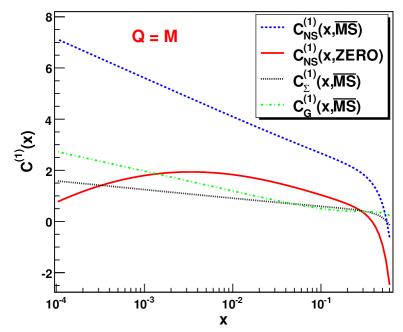
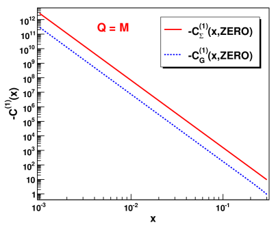
Figure 1: Coefficient functions corresponding to the structure function $F_{2}\!\left(x,Q^{2}\right)$ in the $\overline{\rm MS}$ and ZERO factorization scheme for $n_{\rm f}=3$. Note that because of the logarithmic scale, the coefficient functions in the right graph are plotted with the negative sign.

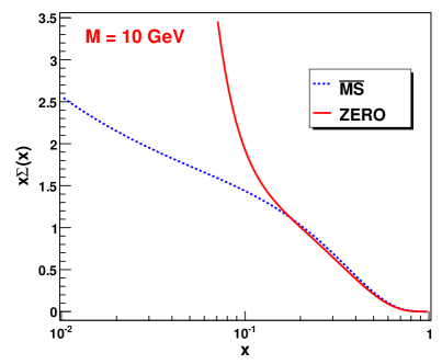
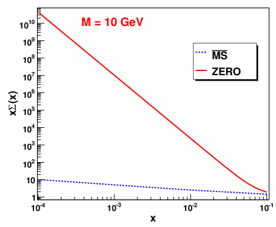
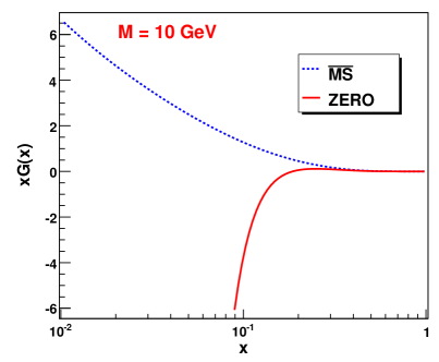
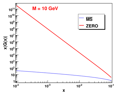
Figure 2: Quark singlet and gluon distribution function in the $\overline{\rm MS}$ and ZERO factorization scheme for $n_{\rm f}=3$. Note that the gluon distribution functions in the lower right graph are plotted in their absolute value — whereas the $\overline{\rm MS}$ distribution is positive, the ZERO distribution is negative (see the lower left graph).

The right graph in Figure 1 shows that the quark singlet and gluon NLO coefficient function behave for low $x$ in the same way as the functions $T^{(1)}_{ij}(x,\overline{\rm MS},{\rm ZERO})$, and the same is true for the quark singlet and gluon distribution function, as can be seen from Figure 2. The low $x$ behaviour of these distribution functions implies that if some physical quantity depends on the values of these distribution functions in the region $x\lesssim 0.1$, then obtaining a reasonable theoretical prediction for this quantity requires a considerable mutual cancellation of large values in the appropriate formula. It is likely that the sufficient cancellation occurs, if ever, only for some choices of the renormalization and factorization scale, which means that most of the choices result in unreliable theoretical predictions. Moreover, the sufficient cancellation causes complications in numerical computations, which can be hardly soluble.

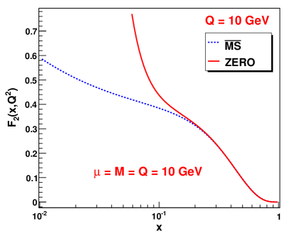
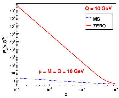
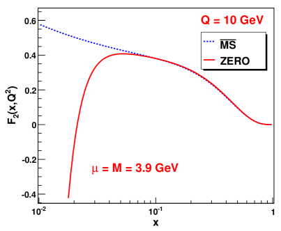
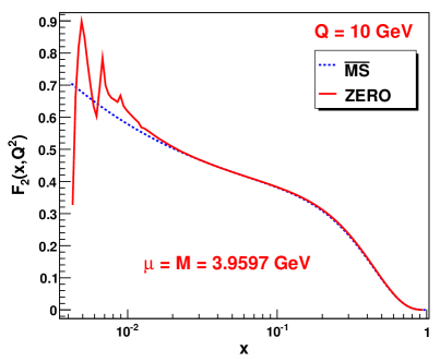
Figure 3: Theoretical predictions for $F_{2}\!\left(x,Q^{2}\right)$ in the $\overline{\rm MS}$ and ZERO factorization scheme for $n_{\rm f}=3$.

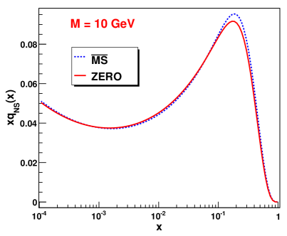
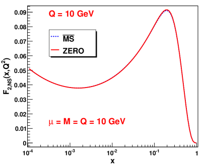
Figure 4: Quark non-singlet distribution function and the non-singlet contribution $F_{2,{\rm NS}}\!\left(x,Q^{2}\right)$ to $F_{2}\!\left(x,Q^{2}\right)$ in the $\overline{\rm MS}$ and ZERO factorization scheme for $n_{\rm f}=3$.

Both undesirable facts manifest themselves in Figure 3. The upper graphs show a theoretical prediction for $F_{2}\!\left(x,Q^{2}\right)$, which is unreliable for $x\lesssim 0.1$. In this case, the theoretically predicted $F_{2}\!\left(x,Q^{2}\right)$ rapidly grows with decreasing $x$ in the region $x\lesssim 0.1$. The lower left graph indicates that there are some theoretical predictions for $F_{2}\!\left(x,Q^{2}\right)$ which rapidly fall with decreasing $x$. Hence, the range of the theoretical predictions for $F_{2}\!\left(x,Q^{2}\right)$ is very large for $x\lesssim 0.1$, and therefore the ZERO factorization scheme for $n_{\rm f}=3$ has practically no predictive power in the region $x\lesssim 0.1$. The range of the theoretical predictions for $F_{2}\!\left(x,Q^{2}\right)$ should include reasonable values, which means that for a given $x_{0}$, there exist such choices of the renormalization and factorization scale that the corresponding theoretical predictions for the value of $F_{2}\!\left(x_{0},Q^{2}\right)$ are reasonable (but this does not mean that there must be such a choice of the renormalization and factorization scale that the corresponding theoretical prediction for $F_{2}\!\left(x,Q^{2}\right)$ is reasonable for all $x$). However, obtaining the reasonable theoretical predictions in numerical calculations is difficult, which can be seen in the lower right graph, where the used precision of the numerical computation is insufficient for $x\lesssim 0.02$. The comparison of the lower graphs shows that the reasonable theoretical predictions in the region $x\lesssim 0.1$ are very sensitive to the choice of the renormalization and factorization scale, which is a consequence of the sensitivity of the extent of the mutual cancellation of large values to this choice.

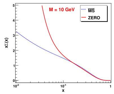
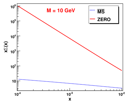
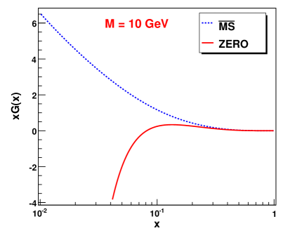
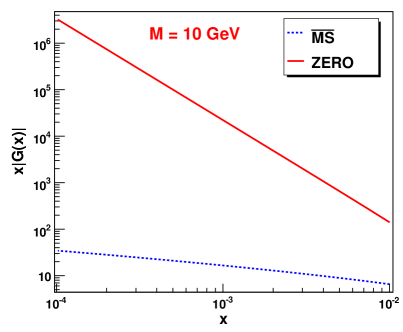
Figure 5: Quark singlet and gluon distribution function in the $\overline{\rm MS}$ and ZERO factorization scheme for $n_{\rm f}=5$. Note that the gluon distribution functions in the lower right graph are plotted in their absolute value — whereas the $\overline{\rm MS}$ distribution is positive, the ZERO distribution is negative (see the lower left graph).

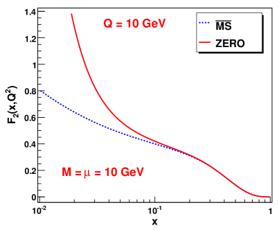
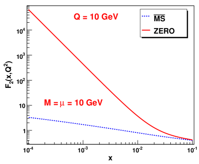
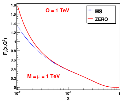
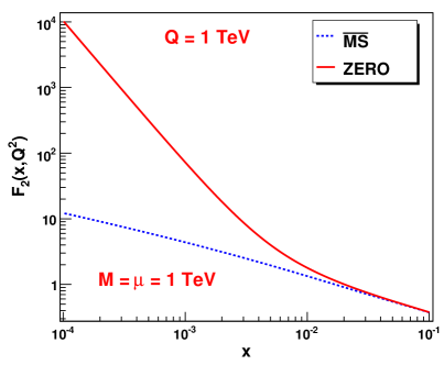
Figure 6: Theoretical predictions for $F_{2}\!\left(x,Q^{2}\right)$ in the $\overline{\rm MS}$ and ZERO factorization scheme for $n_{\rm f}=5$.

According to Subsection 4.4, the ZERO factorization scheme should have no restrictions on its practical applicability in the non-singlet case, which is demonstrated in Figure 4.

The functions $T^{(1)}_{ij}(x,\overline{\rm MS},{\rm ZERO})$ were not calculated in the $x$-space for five (massless) quark flavours. Since the ZERO factorization scheme for $n_{\rm f}=5$ does not satisfy the condition (51), the functions $T^{(1)}_{ij}(x,\overline{\rm MS},{\rm ZERO})$ should behave for low $x$ in the following way (see (50)):

$$T^{(1)}_{ij}(x,\overline{\rm MS},{\rm ZERO})\approx C_{ij}x^{-\xi},\qquad\xi\doteq 3.18,$$ (64)

which indicates that the ZERO factorization scheme has some constraints on its practical applicability, similarly as in the case of $n_{\rm f}=3$ and $n_{\rm f}=4$. The ZERO parton distribution functions and the theoretical predictions for $F_{2}\!\left(x,Q^{2}\right)$ were calculated in a similar way as in the case of $n_{\rm f}=3$ (the only difference was the fact that the value of the factorization scale $M_{\rm T}$ was $10^{7}\,{\rm GeV}$ and the $\overline{\rm MS}$ parton distribution functions corresponded to the MSTW 2008 set mstw ). The ZERO parton distribution functions displayed in Figure 5 behave for low $x$ in a similar way as in the case of $n_{\rm f}=3$, which is displayed in Figure 2. The main difference is the rate of the growth, which is in accordance with relation (64) and is thus slower than in the case of $n_{\rm f}=3$. The comparison of Figures 2 and 5 also shows that in the case of $n_{\rm f}=5$, the rapid growth occurs at a bit lower value of $x$. However, the difference is not significant. Hence, it is not surprising that the ZERO factorization scheme for $n_{\rm f}=5$ gives unreliable theoretical predictions for $F_{2}\!\left(x,Q^{2}\right)$ in the region of low $x$, as can be seen in Figure 6. The comparison of the upper and lower graphs in Figure 6 shows that the region of the practical applicability increases slowly with increasing energy, which also holds for $n_{\rm f}=3$.

For the number of massless quark flavours from three to five, which represents the relevant values for QCD phenomenology, the ZERO factorization scheme is fully applicable for the physical quantities that do not depend on the values of the quark singlet and gluon distribution function in the region $x\lesssim x_{0}$ where $x_{0}=0.1$. However, in the case of the physical quantities which depend on the values of these distribution functions in the region $x\lesssim x_{0}$, the ZERO factorization scheme gives unreliable theoretical predictions and has little predictive power. Even for these physical quantities, obtaining reasonable theoretical predictions is possible for some special choices of the renormalization and factorization scale, but requires a considerable mutual cancellation of large values, which causes difficulties in numerical calculations. In some cases, the value of the bound $x_{0}$ can be lowered, however, it is practically impossible to lower the value of $x_{0}$ in such a way that the ZERO factorization scheme would be applicable in the full range that is used in QCD phenomenology because the extent of the undesirable features rapidly grows with decreasing $x_{0}$.

As it has already been mentioned, the ZERO factorization scheme puts all NLO corrections into hard scattering cross-sections and is therefore a certain opposite to the DIS factorization scheme, in which all NLO corrections (to $F_{2}\!\left(x,Q^{2}\right)$) are included in the corresponding NLO splitting functions. The restricted practical applicability of the ZERO factorization scheme is thus surprising because the DIS factorization scheme can be applied without any restrictions.

There are other reasons why the restricted practical applicability of the ZERO factorization scheme is unexpected and not obvious. As it has already been shown, the ZERO factorization scheme has no restrictions of its practical applicability in the non-singlet case. In addition, the condition of practical applicability (eq. (51)) is nontrivial and its consequences depend on the number of massless quark flavours (e.g. the growth of the ZERO quark singlet distribution function in the low $x$ region is a result of the fact that the ZERO factorization scheme does not satisfy the condition of practical applicability and the rate of this growth depends nontrivially on the number of massless quark flavours (see Figures 2 and 5)).

6 Summary and conclusion

In this text, we have analysed the freedom associated with factorization in massless perturbative QCD, with the emphasis on its quantification. We have derived the formulae that are useful for changing the unphysical quantities associated with the renormalization and factorization procedure and we have shown that factorization schemes can be specified using the higher order splitting functions, which can be chosen at will. This allows us to introduce the so called ZERO factorization scheme, which is defined by setting the higher order splitting functions equal to zero, which means that the ZERO factorization scheme represents a certain opposite to the more familiar DIS factorization scheme. The potential exploitation of the ZERO factorization scheme for the construction of consistent NLO Monte Carlo event generators in which initial state parton showers can be taken formally at the LO has provided the main motivation for this study. The related questions have been discussed in more detail at the end of Section 2.

The discussion of the practical applicability of general factorization schemes has shown that the factorization schemes specified by splitting functions can have unexpected restrictions on its practical applicability. Even if splitting functions appear at first sight as reasonable, they can specify such a factorization scheme that the values of the appropriate parton distribution functions are significantly larger in the low $x$ region than in the case of the standard $\overline{\rm MS}$ factorization scheme. The cancellation of these large values, which has to occur in the expressions for physical quantities, can then result in unreliable theoretical predictions, little predictive power and difficulties in numerical calculations, which restricts the practical applicability of such a factorization scheme.

The question of the practical applicability of general factorization schemes has been studied in more detail at the NLO. We have found the condition (eq. (51)) that must be satisfied by NLO splitting functions in order that any unexpected restrictions on the practical applicability of the corresponding factorization scheme are ruled out. Unfortunately, this condition is not satisfied for the ZERO factorization scheme. The numerical analysis of the ZERO factorization scheme at the NLO has then shown that its application is reliable for the physical quantities which do not depend on the values of the quark singlet and gluon distribution function in the region $x\lesssim 0.1$. However, if we apply the ZERO factorization scheme for the other physical quantities (i.e. those which depend on the values of these distribution functions in the region $x\lesssim 0.1$), then the undesirable features mentioned in the preceding paragraph can occur. The restricted practical applicability of the ZERO factorization scheme has been illustrated on the structure function $F_{2}\!\left(x,Q^{2}\right)$ in the low $x$ region. However, even for the physical quantities for which the ZERO factorization scheme is unreliable, there should exist some special choices of the renormalization and factorization scale that result in reasonable theoretical predictions, but the exploitation of this fact in Monte Carlo event generators is practically impossible because obtaining reasonable theoretical predictions in this case requires a considerable mutual cancellation of large values.

Although the ZERO factorization scheme has some restrictions of its practical applicability, its phenomenological exploitation still makes sense because it can be applied for the description of the production of heavy objects, which is important in searches for new physics.

Appendix A Mellin transform and related formulae

The Mellin transform of a function $f(x)$ defined on the interval $(0,1)$ is given as

$$f(n)=\int_{0}^{1}x^{n-1}f(x)\,{\rm d}x$$ (65)

where $n$ is in general a complex number. The preceding integral, if exists at least for some real value of $n$, defines a function of complex variable $n$ that is holomorphic at least in some right half plane. Using analytical continuation, the Mellin moments $f(n)$ (i.e. the Mellin transform of the function $f(x)$) can be defined even for some values of $n$ for which the integral does not exist (however, this does not mean that the Mellin moments can be defined for all $n$). The Mellin moments $f(n)$ uniquely determine the original function $f(x)$, and therefore the Mellin transform can be inverted. The Mellin transform and its inversion are linear. The formula for the inverse Mellin transform reads

$$f(x)=\frac{1}{2\pi{\rm i}}\int_{\xi-{\rm i}\infty}^{\xi+{\rm i}\infty}f(n)x^{-n}{\rm d}n$$ (66)

where $\xi$ is a real parameter chosen in such a way that the integration contour is located to the right of all singularities of $f(n)$ in the plane of complex $n$.

The location of the singularities of the Mellin moments $f(n)$ is related to the behaviour of the function $f(x)$ in the vicinity of $x=0$. If the Mellin moments $f(n)$ have some singularity for $\operatorname{Re}n>\xi$ and if there exists a nonnegative integer $k$ such that the function $g(x)=(1-x)^{k}f(x)$ is bounded on some interval $[\varepsilon,1]$, then there is no real number $C$ such that

$$|f(x)|\leq C\!\left(\frac{1}{x}\right)^{\!\xi}\,\text{ for }\,x\in(0,\varepsilon)$$ (67)

because if the preceding relation held for some real number $C$, then the function $g(x)$ would have to satisfy

$$|g(x)|\leq K\!\left(\frac{1}{x}\right)^{\!\xi}$$ (68)

for some real number $K$ and for all $x$ from the interval $(0,1]$. This constraint would then imply the following bound

$$|g(n)|\leq\int_{0}^{1}|x^{n-1}||g(x)|{\rm d}x\leq K\!\int_{0}^{1}x^{\operatorname{Re}n-1-\xi}{\rm d}x,$$ (69)

which would mean that the Mellin moments $g(n)$ could not have any singularity for $\operatorname{Re}n>\xi$, but this would be in contradiction with the assumption that the Mellin moments $f(n)$ have some singularity for $\operatorname{Re}n>\xi$ because

$$g(n)=\int_{0}^{1}x^{n-1}\sum_{j=0}^{k}(-1)^{j}\binom{k}{j}x^{j}f(x)\,{\rm d}x=\sum_{j=0}^{k}(-1)^{j}\binom{k}{j}f(n+j).$$ (70)

Some relations concerning factorization (e.g. the relation between dressed and bare parton distribution functions) are expressed as a convolution given by

$$\left(f\ast g\right)\!(x) =\int_{0}^{1}\!\int_{0}^{1}\!{\rm d}y{\rm d}z\,f(y)g(z)\delta(yz-x)=$$ (71)

$$=\int_{x}^{1}\frac{{\rm d}y}{y}\,f\!\left(\frac{x}{y}\right)\!g(y)=\int_{x}^{1}\frac{{\rm d}y}{y}\,f(y)\>\!g\!\left(\frac{x}{y}\right)\!.$$ (72)

From formula (71), we easily get

$$\left(f\ast g\right)\!(n)=f(n)g(n),$$ (73)

which means that the Mellin transform converts the convolution (71) to ordinary multiplication of Mellin moments.

Using formula (71), we find

$$\int_{0}^{1}\!{\rm d}x\,f(x)\left(g\ast h\right)\!(x) =\int_{0}^{1}\!\int_{0}^{1}\!{\rm d}y{\rm d}z\,f(yz)g(y)h(z)=$$

$$=\int_{0}^{1}\!{\rm d}x\left(f\otimes g\right)\!(x)h(x)=\int_{0}^{1}\!{\rm d}x\left(f\otimes h\right)\!(x)g(x)$$ (74)

where the symbol $\otimes$ is defined as

$$\left(f\otimes g\right)\!(x)=\int_{0}^{1}\!{\rm d}y\,f(xy)g(y)$$ (75)

and satisfies

$$\left[\left(f\otimes g\right)\otimes h\right]\!(x) =\int_{0}^{1}\!{\rm d}z\left(f\otimes g\right)\!(xz)h(z)=\int_{0}^{1}\!\int_{0}^{1}\!{\rm d}y{\rm d}z\,f(xyz)g(y)h(z)=$$

$$=\int_{0}^{1}\!\int_{0}^{1}\!{\rm d}y{\rm d}z\,g(y)h(z)\int_{0}^{1}\!{\rm d}\xi\,f(x\xi)\delta(\xi-yz)=$$

$$=\int_{0}^{1}\!{\rm d}\xi\,f(x\xi)\int_{0}^{1}\!\int_{0}^{1}\!{\rm d}y{\rm d}z\,g(y)h(z)\delta(\xi-yz)=$$

$$=\int_{0}^{1}\!{\rm d}\xi\,f(x\xi)\left(g\ast h\right)\!(\xi)=\left[f\otimes\left(g\ast h\right)\right]\!(x).$$ (76)

Formulae (74) and (76) are useful for manipulations with expressions for cross-sections.

Using relations (65), (71) and (75), we easily get the following properties of the function $f(x)=\delta(1-x)$:

$$f(n)=1,\qquad f\ast g=g\ast f=g,\qquad g\otimes f=g$$ (77)

where $g$ is an arbitrary function.

Appendix B Some important formulae for the QCD coupling parameter $a(\mu,{\rm RS})$

B.1 Changing expansion parameter

Within the framework of perturbative QCD, the QCD coupling parameter $a(\mu,{\rm RS})$ is a function of the renormalization scale $\mu$ and the renormalization scheme RS. Hence, it is useful to be familiar with relations between coupling parameters corresponding to different arguments.

Consider an expansion parameter $a(P)$ depending on a set of parameters denoted by $P$. Let us assume that the relation between expansion parameters corresponding to different sets of parameters $P_{1}$ and $P_{2}$ has the form of power series:

$$a(P_{1})=\sum_{l=0}^{\infty}c^{(1)}_{l}(P_{1},P_{2})\,a^{l+1}(P_{2}).$$ (78)

This relation can then be generalized as follows:

$$a^{k}(P_{1})=\sum_{l=0}^{\infty}c^{(k)}_{l}(P_{1},P_{2})\,a^{l+k}(P_{2})$$ (79)

where $k$ is a nonnegative integer and

$$c^{(0)}_{l}(P_{1},P_{2}) =\delta_{l0},$$ (80)

$$c^{(k+1)}_{l}(P_{1},P_{2}) =\sum_{m=0}^{l}c^{(k)}_{l-m}(P_{1},P_{2})\,c^{(1)}_{m}(P_{1},P_{2})\quad\text{for}\quad k\geq 1.$$ (81)

Formula (79) is useful for changing an expansion parameter of power expansions. Consider some quantity $F$ which can be expressed as an expansion in powers of $a(P_{0})$:

$$F=\sum_{k=0}^{\infty}F^{(k)}(P_{0})\,a^{k+k_{0}}(P_{0}).$$ (82)

Using formula (79), we can then obtain an expansion of $F$ in powers of an arbitrary expansion parameter $a(P)$:

$$F=\sum_{k=0}^{\infty}F^{(k)}(P)\,a^{k+k_{0}}(P)$$ (83)

where

$$F^{(k)}(P)=\sum_{l=0}^{k}F^{(l)}(P_{0})\,c^{(l+k_{0})}_{k-l}(P_{0},P).$$ (84)

B.2 The QCD coupling parameter in $d=4-2\varepsilon$ space-time dimensions

Within the framework of dimensional regularization in $d=4-2\varepsilon$ space-time dimensions, equation (1), which describes the dependence of the QCD coupling parameter $a(\mu,{\rm RS})$ on the renormalization scale $\mu$, has the following form

$$\frac{{\rm d}a(\mu,{\rm RS})}{{\rm d}\ln\mu}=\sum_{l=0}^{\infty}\beta_{l}({\rm RS})\,a^{l+1}(\mu,{\rm RS})$$ (85)

where $\beta_{0}({\rm RS})=-2\varepsilon$ and all higher order coefficients $\beta_{l}({\rm RS})$, $l\geq 1$ are linear functions of $\varepsilon$ and depend on the renormalization scheme RS (in the case of the coefficients $\beta_{1}({\rm RS})$ and $\beta_{2}({\rm RS})$, only the part proportional to $\varepsilon$ is dependent on the renormalization scheme RS).

The renormalization scale of the QCD coupling parameter can be changed using the formula

$$a(\mu,{\rm RS})=\sum_{l=0}^{\infty}g^{(1)}_{l}(\mu,\mu_{0},{\rm RS})\,a^{l+1}(\mu_{0},{\rm RS}),$$ (86)

which can be derived from (85). The coefficients $g^{(1)}_{l}(\mu,\mu_{0},{\rm RS})$ depend on $\varepsilon$ and are finite in the limit $\varepsilon\to 0$. The change of the renormalization scheme of the QCD coupling parameter is then described by the formula

$$a(\mu,{\rm RS}_{1})=\sum_{l=0}^{\infty}h^{(1)}_{l}({\rm RS}_{1},{\rm RS}_{2})\,a^{l+1}(\mu,{\rm RS}_{2}),\quad h^{(1)}_{0}({\rm RS}_{1},{\rm RS}_{2})=1.$$ (87)

Contrary to the coefficients $g^{(1)}_{l}(\mu,\mu_{0},{\rm RS})$, the coefficients $h^{(1)}_{l}({\rm RS}_{1},{\rm RS}_{2})$ are independent of $\varepsilon$. Both formulae (86) and (87) have the form of (78) and can thus be generalized to

$$a^{k}(\mu,{\rm RS}) =\sum_{l=0}^{\infty}g^{(k)}_{l}(\mu,\mu_{0},{\rm RS})\,a^{l+k}(\mu_{0},{\rm RS}),$$ (88)

$$a^{k}(\mu,{\rm RS}_{1}) =\sum_{l=0}^{\infty}h^{(k)}_{l}({\rm RS}_{1},{\rm RS}_{2})\,a^{l+k}(\mu,{\rm RS}_{2}),$$ (89)

where the coefficients $g^{(k)}_{l}(\mu,\mu_{0},{\rm RS})$ and $h^{(k)}_{l}({\rm RS}_{1},{\rm RS}_{2})$ are determined by relations (80) and (81).

Appendix C Solution of equations (126) and (21, 130)

This appendix contains formulae for the solution of the matrix equation

$$\left[\mathbf{X}(n),\mathbf{P}^{(0)}(n)\right]-\kappa\mathbf{X}(n)=\mathbf{Y}(n),\quad\kappa\neq 0$$ (90)

with respect to $\mathbf{X}(n)$. The matrix $\mathbf{P}^{(0)}(n)$ represents the LO splitting functions and the matrix $\mathbf{Y}(n)$ is given. All three matrices in the preceding equation are square matrices with indices corresponding to parton species: $q_{i}$, $\bar{q}_{i}$ and $G$, and therefore their dimension is $2n_{\rm f}+1$ where $n_{\rm f}$ denotes the number of quark flavours. For the following, it is useful to introduce a unified labeling for quarks and antiquarks: $Q_{i}=q_{i}$, $Q_{i+n_{\rm f}}=\bar{q}_{i}$. The structure of the matrix $\mathbf{P}^{(0)}(n)$ can then be expressed as follows:

$$P^{(0)}_{Q_{i}Q_{j}}(n)=P^{(0)}_{qq}(n)\delta_{ij},\quad P^{(0)}_{Q_{i}G}(n)=P^{(0)}_{qG}(n),\quad P^{(0)}_{GQ_{i}}(n)=P^{(0)}_{Gq}(n),\quad P^{(0)}_{GG}(n).$$ (91)

For better readability of the formulae expressing the solution of equation (90), it is convenient not to write out explicitly the dependence on $n$. The formulae then read

$$X_{Q_{i}Q_{j}}={} \overline{X}-\frac{1}{\kappa}Y_{Q_{i}Q_{j}}+\frac{P^{(0)}_{qG}P^{(0)}_{Gq}\left(\sum_{k=1}^{2n_{\rm f}}Y_{Q_{i}Q_{k}}-Y_{qq}\right)+\kappa P^{(0)}_{Gq}\left(Y_{Q_{i}G}-Y_{qG}\right)}{\kappa\left(\kappa P^{(0)}_{GG}-\kappa P^{(0)}_{qq}-\kappa^{2}+2n_{\rm f}P^{(0)}_{qG}P^{(0)}_{Gq}\right)}+{}$$

$${}+\frac{P^{(0)}_{qG}P^{(0)}_{Gq}\left(\sum_{k=1}^{2n_{\rm f}}Y_{Q_{k}Q_{j}}-Y_{qq}\right)-\kappa P^{(0)}_{qG}\left(Y_{GQ_{j}}-Y_{Gq}\right)}{\kappa\left(\kappa P^{(0)}_{qq}-\kappa P^{(0)}_{GG}-\kappa^{2}+2n_{\rm f}P^{(0)}_{qG}P^{(0)}_{Gq}\right)},$$ (92)

$$X_{Q_{i}G}={} X_{qG}+\frac{\kappa\left(Y_{Q_{i}G}-Y_{qG}\right)+P^{(0)}_{qG}\left(\sum_{k=1}^{2n_{\rm f}}Y_{Q_{i}Q_{k}}-Y_{qq}\right)}{\kappa P^{(0)}_{GG}-\kappa P^{(0)}_{qq}-\kappa^{2}+2n_{\rm f}P^{(0)}_{qG}P^{(0)}_{Gq}},$$ (93)

$$X_{GQ_{i}}={} X_{Gq}+\frac{\kappa\left(Y_{GQ_{i}}-Y_{Gq}\right)-P^{(0)}_{Gq}\left(\sum_{k=1}^{2n_{\rm f}}Y_{Q_{k}Q_{i}}-Y_{qq}\right)}{\kappa P^{(0)}_{qq}-\kappa P^{(0)}_{GG}-\kappa^{2}+2n_{\rm f}P^{(0)}_{qG}P^{(0)}_{Gq}},$$ (94)

$$X_{GG}={} -\frac{1}{\kappa}Y_{GG}-2n_{\rm f}\overline{X}$$ (95)

where

$$\overline{X} =\frac{1}{\nu}\left[P^{(0)}_{Gq}\left(P^{(0)}_{qq}-P^{(0)}_{GG}-\kappa\right)Y_{qG}+P^{(0)}_{qG}\left(P^{(0)}_{qq}-P^{(0)}_{GG}+\kappa\right)Y_{Gq}-{}\right.$$

$$\quad\left.{}-2P^{(0)}_{qG}P^{(0)}_{Gq}\left(Y_{qq}-Y_{GG}\right)\right]\!,$$ (96)

$$X_{qG} =\frac{1}{\nu}\left[\left(P^{(0)}_{qq}-P^{(0)}_{GG}-\kappa\right)\left(\kappa Y_{qG}+P^{(0)}_{qG}\left(Y_{qq}-Y_{GG}\right)\right)+{}\right.$$

$$\quad\left.{}+4n_{\rm f}P^{(0)}_{qG}\left(P^{(0)}_{Gq}Y_{qG}+P^{(0)}_{qG}Y_{Gq}\right)\right]\!,$$ (97)

$$X_{Gq} =\frac{1}{\nu}\left[\left(P^{(0)}_{GG}-P^{(0)}_{qq}-\kappa\right)\left(\kappa Y_{Gq}-P^{(0)}_{Gq}\left(Y_{qq}-Y_{GG}\right)\right)+{}\right.$$

$$\quad\left.{}+4n_{\rm f}P^{(0)}_{Gq}\left(P^{(0)}_{Gq}Y_{qG}+P^{(0)}_{qG}Y_{Gq}\right)\right]$$ (98)

and the denominator $\nu$ is given as

$$\nu=\kappa\left(\kappa^{2}-\left(P^{(0)}_{qq}-P^{(0)}_{GG}\right)^{2}-8n_{\rm f}P^{(0)}_{qG}P^{(0)}_{Gq}\right)\!.$$ (99)

The symbols $Y_{qq}$, $Y_{qG}$ and $Y_{Gq}$ are defined as follows:

$$Y_{qq}\equiv\frac{1}{2n_{\rm f}}\sum_{k,l=1}^{2n_{\rm f}}Y_{Q_{k}Q_{l}},\quad Y_{qG}\equiv\frac{1}{2n_{\rm f}}\sum_{k=1}^{2n_{\rm f}}Y_{Q_{k}G},\quad Y_{Gq}\equiv\frac{1}{2n_{\rm f}}\sum_{k=1}^{2n_{\rm f}}Y_{GQ_{k}}.$$ (100)

If all denominators in expressions (92)–(98) are nonzero, then the solution of equation (90) exists and is unique for an arbitrary right hand side $\mathbf{Y}$.

It can be shown that for every nonzero $\kappa$, there exists some right half plane in which all denominators in expressions (92)–(98) are nonzero. Hence, if the right hand side $\mathbf{Y}(n)$ of (90) is holomorphic in some right half plane, then there exists some right half plane in which the solution $\mathbf{X}(n)$ of equation (90) is unique and holomorphic.

Appendix D Analysis of the freedom associated with factorization in massless QCD

This appendix contains a detailed analysis of the freedom associated with the factorization procedure in massless perturbative QCD. Important results of this appendix are summarized in Subsections 3.2 and 3.3.

To investigate the ambiguity associated with the definition of dressed parton distribution functions, it is useful to express the relevant formulae in terms of Mellin moments, which are defined in Appendix A. Converting relation (13) into the space of Mellin moments, we get ordinary matrix multiplication of moments

$$\mathbf{D}(n,M,{\rm FS},{\rm RS})=\mathbf{A}(n,M,{\rm FS},{\rm RS})\mathbf{\widehat{D}}(n)$$ (101)

and the expansion of $\mathbf{A}(n,M,{\rm FS},{\rm RS})$ is expressed as follows

$$\mathbf{A}(n,M,{\rm FS},{\rm RS})=\sum_{k=0}^{\infty}a^{k}(M,{\rm RS})\mathbf{A}\!^{(k)}(n,{\rm FS},{\rm RS}),\quad\mathbf{A}\!^{(0)}(n,{\rm FS},{\rm RS})=\mathbf{1}.$$ (102)

The form of relation (101) allows us to obtain expression for the bare parton distribution functions $\mathbf{\widehat{D}}(n)$:

$$\mathbf{\widehat{D}}(n)=\mathbf{B}(n,M,{\rm FS},{\rm RS})\mathbf{D}(n,M,{\rm FS},{\rm RS})$$ (103)

where $\mathbf{B}(n,M,{\rm FS},{\rm RS})$ is the matrix inversion of $\mathbf{A}(n,M,{\rm FS},{\rm RS})$, which can be expanded in powers of $a(M,{\rm RS})$:

$$\mathbf{B}(n,M,{\rm FS},{\rm RS})=\sum_{k=0}^{\infty}a^{k}(M,{\rm RS})\mathbf{B}^{(k)}(n,{\rm FS},{\rm RS})$$ (104)

where the coefficients $\mathbf{B}^{(k)}(n,{\rm FS},{\rm RS})$ are determined by the following recurrence relation

$$\mathbf{B}^{(k)}(n,{\rm FS},{\rm RS})=-\sum_{l=0}^{k-1}\mathbf{A}\!^{(k-l)}(n,{\rm FS},{\rm RS})\mathbf{B}^{(l)}(n,{\rm FS},{\rm RS}),\quad\mathbf{B}^{(0)}(n,{\rm FS},{\rm RS})=\mathbf{1},$$ (105)

which implies that $\mathbf{B}^{(k)}(n,{\rm FS},{\rm RS})$ is given as a sum of terms of the form

$$c\mathbf{A}\!^{(l_{1})}(n,{\rm FS},{\rm RS})\mathbf{A}\!^{(l_{2})}(n,{\rm FS},{\rm RS})\dotsm\mathbf{A}\!^{(l_{m})}(n,{\rm FS},{\rm RS})$$ (106)

where the coefficient $c$ is an integer and $\sum\limits_{i=1}^{m}l_{i}=k$. This means that $\mathbf{B}^{(k)}(n,{\rm FS},{\rm RS})$ depends on $\mathbf{A}^{(l)}(n,{\rm FS},{\rm RS})$ for $1\leq l\leq k$ and is independent of $\mathbf{A}^{(l)}(n,{\rm FS},{\rm RS})$ for $l>k$. Relation (105) and its consequence are useful for analyzing formulae (114) and (120).

The following three subsections will be devoted to changing the unphysical quantities on which the dressed parton distribution functions depend. The obtained results will then allow us to investigate the dependence of the splitting functions and the hard scattering cross-sections on the unphysical quantities associated with the factorization procedure.

D.1 Changing the renormalization scheme

If we want to change the renormalization scheme used for the factorization procedure from ${\rm RS}_{1}$ to ${\rm RS}_{2}$, then we should convert the expansion parameter $a(M,{\rm RS}_{1})$ to $a(M,{\rm RS}_{2})$. Hence, let us express $A_{ij}(x,M,{\rm FS},{\rm RS}_{1})$ as an expansion in powers of $a(M,{\rm RS}_{2})$:

$$A_{ij}(x,M,{\rm FS},{\rm RS}_{1})=\delta_{ij}\delta(1-x)+{}\\ {}+\sum_{k=1}^{\infty}a^{k}(M,{\rm RS}_{2})\sum_{l=1}^{k}h^{(l)}_{k-l}({\rm RS}_{1},{\rm RS}_{2})\,A_{ij}^{(l)}(x,{\rm FS},{\rm RS}_{1}),$$ (107)

where we have used formula (89). Seeing that the coefficients $h^{(k)}_{l}({\rm RS}_{1},{\rm RS}_{2})$ are independent of $\varepsilon$, the preceding expansion has the form that is consistent with formulae (14) and (15), and therefore there must exist such a factorization scheme $\mathcal{FS}({\rm RS}_{1},{\rm RS}_{2},{\rm FS})$ that

$$A_{ij}(x,M,{\rm FS},{\rm RS}_{1})=A_{ij}(x,M,\mathcal{FS}({\rm RS}_{1},{\rm RS}_{2},{\rm FS}),{\rm RS}_{2}).$$ (108)

The pair of $\{{\rm FS},{\rm RS}_{1}\}$ thus defines, independently of the factorization scale $M$, the same singular factors that are absorbed into parton distribution functions as the pair of $\{\mathcal{FS}({\rm RS}_{1},{\rm RS}_{2},{\rm FS}),{\rm RS}_{2}\}$, and therefore both pairs are equivalent in the sense of the definition of dressed parton distribution functions. Changing the renormalization scheme from ${\rm RS}_{0}$ to RS for the fixed factorization scheme FS and factorization scale $M$ can thus be converted to changing the factorization scheme FS to the factorization scheme $\mathcal{FS}({\rm RS},{\rm RS}_{0},{\rm FS})$ for the fixed renormalization scheme ${\rm RS}_{0}$ and factorization scale $M$. The change of the factorization scheme will be discussed in Subsection D.3.

In order to be able to change the renormalization scheme in the above described manner, we have to know some prescription for the determination of the factorization scheme $\mathcal{FS}({\rm RS}_{1},{\rm RS}_{2},{\rm FS})$. Such a prescription can be obtained as follows. Comparing the expansion (14) of the right hand side of (108) with the expansion (107) of the left hand side of (108), we find

$$A_{ij}^{(k)}(x,\mathcal{FS}({\rm RS}_{1},{\rm RS}_{2},{\rm FS}),{\rm RS}_{2})=\sum_{l=1}^{k}h^{(l)}_{k-l}({\rm RS}_{1},{\rm RS}_{2})\,A^{(l)}_{ij}(x,{\rm FS},{\rm RS}_{1}),\quad k\geq 1.$$ (109)

Using formula (15) and exploiting the fact that the coefficients $h^{(k)}_{l}({\rm RS}_{1},{\rm RS}_{2})$ are independent of $\varepsilon$, we get

$$A_{ij}^{(km)}(x,\mathcal{FS}({\rm RS}_{1},{\rm RS}_{2},{\rm FS}),{\rm RS}_{2})=\sum_{l=1}^{k}h^{(l)}_{k-l}({\rm RS}_{1},{\rm RS}_{2})\,A^{(lm)}_{ij}(x,{\rm FS},{\rm RS}_{1})$$ (110)

where $k\geq 1$ and $m\geq 0$. The desired prescription is then represented by the preceding equation (110) for $m=0$.

D.2 Evolution equations

The evolution equations describe the dependence of dressed parton distribution functions on the factorization scale. From formula (101), we get

$$\frac{{\rm d}\mathbf{D}(n,M,{\rm FS},{\rm RS})}{{\rm d}\ln M}=\frac{{\rm d}\mathbf{A}(n,M,{\rm FS},{\rm RS})}{{\rm d}\ln M}\mathbf{B}(n,M,{\rm FS},{\rm RS})\mathbf{D}(n,M,{\rm FS},{\rm RS}),$$ (111)

where we have used formula (103) to express the bare parton distribution functions $\mathbf{\widehat{D}}(n)$ in terms of the dressed parton distribution functions $\mathbf{D}(n,M,{\rm FS},{\rm RS})$. Expanding in powers of $a(M,{\rm RS})$, using equation (85) and after some manipulations, we obtain

$$\frac{{\rm d}\mathbf{A}(n,M,{\rm FS},{\rm RS})}{{\rm d}\ln M}\mathbf{B}(n,M,{\rm FS},{\rm RS})=a(M,{\rm RS})\mathbf{P}(n,M,{\rm FS},{\rm RS})$$ (112)

where the splitting functions $\mathbf{P}(n,M,{\rm FS},{\rm RS})$ have an expansion in powers of $a(M,{\rm RS})$

$$\mathbf{P}(n,M,{\rm FS},{\rm RS})=\sum_{k=0}^{\infty}a^{k}(M,{\rm RS})\,\mathbf{P}^{(k)}(n,{\rm FS},{\rm RS})$$ (113)

with the coefficients given by the formula

$$\mathbf{P}^{(k)}(n,{\rm FS},{\rm RS})=\sum_{l=0}^{k}\left(\sum_{p=0}^{l}(p+1)\beta_{l-p}({\rm RS})\mathbf{A}\!^{(p+1)}(n,{\rm FS},{\rm RS})\right)\mathbf{B}^{(k-l)}(n,{\rm FS},{\rm RS}).$$ (114)

The evolution equations expressed in terms of Mellin moments thus read

$$\frac{{\rm d}\mathbf{D}(n,M,{\rm FS},{\rm RS})}{{\rm d}\ln M}=a(M,{\rm RS})\mathbf{P}(n,M,{\rm FS},{\rm RS})\mathbf{D}(n,M,{\rm FS},{\rm RS}).$$ (115)

Converting the preceding equation into $x$-space, we obtain the evolution equations in the form of (3).

The splitting functions $\mathbf{P}^{(k)}(n,{\rm FS},{\rm RS})$, determined by (114), must be finite in the limit $\varepsilon\to 0$. A detailed analysis of this condition shows that

$$\begin{array}[]{l}\mathbf{A}\!^{(kl)}(n,{\rm FS},{\rm RS})=0\text{ for $l>k\geq 1$,}\\[6.0pt] \mathbf{A}\!^{(kl)}(n,{\rm FS},{\rm RS})\text{ for $k\geq l\geq 2$ is uniquely determined by}\\ \mathbf{A}\!^{(m0)}(n,{\rm FS})\text{ and }\mathbf{A}\!^{(m1)}(n,{\rm FS},{\rm RS})\text{ for $1\leq m\leq k-1$.}\end{array}$$ (116)

Since the functions $A^{(k0)}_{ij}(x)$ can be choosen at will, all nontrivial information concerning the properties of the theory has to be contained in the functions $A^{(k1)}_{ij}(x,{\rm FS},{\rm RS})$.

D.3 Changing the factorization scheme

The formula for changing the factorization scheme can be obtained from relations (101) and (103):

$$\mathbf{D}(n,M,{\rm FS}_{1},{\rm RS})=\mathbf{T}(n,M,{\rm FS}_{1},{\rm FS}_{2},{\rm RS})\mathbf{D}(n,M,{\rm FS}_{2},{\rm RS})$$ (117)

where

$$\mathbf{T}(n,M,{\rm FS}_{1},{\rm FS}_{2},{\rm RS})=\mathbf{A}(n,M,{\rm FS}_{1},{\rm RS})\mathbf{B}(n,M,{\rm FS}_{2},{\rm RS}).$$ (118)

Expanding the preceding relation in powers of $a(M,{\rm RS})$, we get

$$\mathbf{T}(n,M,{\rm FS}_{1},{\rm FS}_{2},{\rm RS})=\sum_{k=0}^{\infty}a^{k}(M,{\rm RS})\,\mathbf{T}^{(k)}(n,{\rm FS}_{1},{\rm FS}_{2},{\rm RS})$$ (119)

where the coefficients of the expansion are determined by the formula

$$\mathbf{T}^{(k)}(n,{\rm FS}_{1},{\rm FS}_{2},{\rm RS})=\sum_{l=0}^{k}\mathbf{A}\!^{(k-l)}(n,{\rm FS}_{1},{\rm RS})\mathbf{B}^{(l)}(n,{\rm FS}_{2},{\rm RS}).$$ (120)

Using relation (105), we find that $\mathbf{T}^{(0)}(n,{\rm FS}_{1},{\rm FS}_{2},{\rm RS})=\mathbf{1}$ and $\mathbf{T}^{(k)}(n,{\rm FS}_{1},{\rm FS}_{2},{\rm RS})$ for $k\geq 1$ is given as a polynomial expression in $\mathbf{A}\!^{(l)}(n,{\rm FS}_{1},{\rm RS})$ and $\mathbf{A}\!^{(l)}(n,{\rm FS}_{2},{\rm RS})$ for $1\leq l\leq k$ with coefficients independent of $\varepsilon$. Seeing that $\mathbf{T}^{(k)}(n,{\rm FS}_{1},{\rm FS}_{2},{\rm RS})$ must be finite in the limit $\varepsilon\to 0$, we can do the following replacement

$$\mathbf{A}\!^{(l)}(n,{\rm FS}_{1},{\rm RS})\to\mathbf{A}\!^{(l0)}(n,{\rm FS}_{1}),\quad\mathbf{A}\!^{(l)}(n,{\rm FS}_{2},{\rm RS})\to\mathbf{A}\!^{(l0)}(n,{\rm FS}_{2})$$ (121)

in the expression for $\mathbf{T}^{(k)}(n,{\rm FS}_{1},{\rm FS}_{2},{\rm RS})$ because the singular parts of $\mathbf{A}\!^{(l)}(n,{\rm FS}_{1},{\rm RS})$ and $\mathbf{A}\!^{(l)}(n,{\rm FS}_{2},{\rm RS})$ cannot contribute to the finite part of $\mathbf{T}^{(k)}(n,{\rm FS}_{1},{\rm FS}_{2},{\rm RS})$ (see formula (15)). Hence, $\mathbf{T}^{(k)}(n,{\rm FS}_{1},{\rm FS}_{2},{\rm RS})$ does not depend on the renormalization scheme RS.

The condition that $\mathbf{T}^{(k)}(n,{\rm FS}_{1},{\rm FS}_{2})$ is finite in the limit $\varepsilon\to 0$ allows us to determine the dependence of $\mathbf{A}\!^{(l1)}(n,{\rm FS},{\rm RS})$ on the factorization scheme. Consider the so called minimal subtraction (MS) factorization scheme, which is defined by setting the functions $A^{(k0)}_{ij}(x)$ equal to zero. From relations (15) and (105), we get

$$\mathbf{B}^{(k)}(n,{\rm MS},{\rm RS})=-\frac{1}{\varepsilon}\mathbf{A}\!^{(k1)}(n,{\rm MS},{\rm RS})+\text{terms containing at least $\frac{1}{\varepsilon^{2}}$}.$$ (122)

The requirement of the absence of a term proportional to $1/\varepsilon$ on the right hand side of (120) then implies

$$\mathbf{A}\!^{(k1)}(n,{\rm FS},{\rm RS})=\mathbf{A}\!^{(k1)}(n,{\rm MS},{\rm RS})+\sum_{l=1}^{k-1}\mathbf{A}\!^{(k-l,0)}(n,{\rm FS})\mathbf{A}\!^{(l1)}(n,{\rm MS},{\rm RS}).$$ (123)

This formula determines the dependence of the functions $A^{(k1)}_{ij}(x,{\rm FS},{\rm RS})$ on the arbitrary functions $A^{(k0)}_{ij}(x)$, which specify the factorization scheme. The dependence of the functions $A^{(k1)}_{ij}(x,{\rm MS},{\rm RS})$ on the renormalization scheme is then described by the following formula resulting from (110):

$$A_{ij}^{(k1)}(x,{\rm MS},{\rm RS})=\sum_{l=1}^{k}h^{(l)}_{k-l}({\rm RS}_{0},{\rm RS})\,A^{(l1)}_{ij}(x,{\rm MS},{\rm RS}_{0}),$$ (124)

where we have used the fact that $\mathcal{FS}({\rm RS}_{0},{\rm RS},{\rm MS})={\rm MS}$, which follows from equation (110) for $m=0$. The obtained relations (116), (123) and (124) thus imply that if we know the functions $A_{ij}^{(k1)}(x,{\rm FS},{\rm RS})$ for some factorization scheme and some renormalization scheme, then we are able to determine the complete singular factors $A_{ij}(x,M,{\rm FS},{\rm RS})$ for an arbitrary factorization scale, factorization scheme and renormalization scheme.

Since the pair of $\{{\rm FS},{\rm RS}\}$ is equivalent to the pair of $\{\mathcal{FS}({\rm RS},{\rm RS}_{0},{\rm FS}),{\rm RS}_{0}\}$, we can convert the simultaneous change of the factorization scheme and the renormalization scheme from $\{{\rm FS}_{0},{\rm RS}_{0}\}$ to $\{{\rm FS},{\rm RS}\}$ to changing the factorization scheme from ${\rm FS}_{0}$ to $\mathcal{FS}({\rm RS},{\rm RS}_{0},{\rm FS})$ for the fixed renormalization scheme ${\rm RS}_{0}$.

D.4 Specification of factorization scheme via splitting functions

The relations presented in the preceding subsections allow us to investigate the dependence of the splitting functions on the factorization scheme, which is one of the main aims of this text. This dependence interests us only in the limit $\varepsilon\to 0$ (in four space-time dimensions).

From formula (114), we get that the LO splitting functions for $\varepsilon=0$ are given as

$$\mathbf{P}^{(0)}(x,{\rm FS},{\rm RS})=\lim_{\varepsilon\to 0}\left(-2\varepsilon\mathbf{A}\!^{(1)}(x,{\rm FS},{\rm RS})\right)=-2\mathbf{A}\!^{(11)}(x,{\rm FS},{\rm RS}).$$ (125)

Relations (123), (124) and (87) then imply that $\mathbf{A}\!^{(11)}(x,{\rm FS},{\rm RS})$ is independent of the factorization scheme and the renormalization scheme, and therefore the LO splitting functions $\mathbf{P}^{(0)}(x)$ are unique (for $\varepsilon=0$). However, this is not true for the higher order splitting functions. Using (105), (114), (123), (125) and the properties of the coefficients $\beta_{k}({\rm RS})$ mentioned in Appendix B.2, we find that the higher order splitting functions $\mathbf{P}^{(k)}(n,{\rm FS},{\rm RS})$, $k\geq 1$ for $\varepsilon=0$ are expressed as

$$\mathbf{P}^{(k)}(n,{\rm FS},{\rm RS})=\left[\mathbf{A}\!^{(k0)}(n,{\rm FS}),\mathbf{P}^{(0)}(n)\right]-kb\mathbf{A}\!^{(k0)}(n,{\rm FS})+\mathbf{R}_{k}(n,{\rm FS},{\rm RS})$$ (126)

where $\mathbf{R}_{k}(n,{\rm FS},{\rm RS})$ is a polynomial expression in $\mathbf{A}\!^{(l1)}(n,{\rm MS},{\rm RS})$ for $1\leq l\leq k+1$ and $\mathbf{A}\!^{(l0)}(n,{\rm FS})$ for $1\leq l\leq k-1$ with the coefficients depending on the renormalization scheme RS. The preceding relation (126) and the relations presented in Appendix C imply that for any set of arbitrarily chosen splitting functions $\mathbf{P}^{(l)}(n)$, $1\leq l\leq k$ where $k$ is arbitrary, there exists exactly one set of the corresponding $\mathbf{A}\!^{(l0)}(n)$, $1\leq l\leq k$. The higher order splitting functions $\mathbf{P}^{(k)}(x,{\rm FS},{\rm RS})$, $k\geq 1$ for $\varepsilon=0$ can thus be chosen at will and can be used for labeling factorization schemes.

The specification of factorization schemes via splitting functions can be useful for phenomenology. In order to simplify the application of this kind of specification, it is necessary to derive formulae for expressing $\mathbf{T}^{(k)}(x,{\rm FS}_{1},{\rm FS}_{2})$ and $\mathcal{FS}({\rm RS}_{1},{\rm RS}_{2},{\rm FS})$ in terms of splitting functions. The relation between $\mathbf{T}^{(k)}(x,{\rm FS}_{1},{\rm FS}_{2})$ and the corresponding splitting functions can be obtained as follows. Let us start with the relation

$$\mathbf{A}(n,M,{\rm FS}_{1},{\rm RS})=\mathbf{T}(n,M,{\rm FS}_{1},{\rm FS}_{2},{\rm RS})\mathbf{A}(n,M,{\rm FS}_{2},{\rm RS}),$$ (127)

which follows from (118). Differentiating the preceding relation with respect to $\ln M$ and using equation (112), we find

$$a(M,{\rm RS})\mathbf{P}(n,M,{\rm FS}_{1},{\rm RS})\mathbf{T}(n,M,{\rm FS}_{1},{\rm FS}_{2},{\rm RS})=\frac{{\rm d}\mathbf{T}(n,M,{\rm FS}_{1},{\rm FS}_{2},{\rm RS})}{{\rm d}\ln M}+{}\\ {}+a(M,{\rm RS})\mathbf{T}(n,M,{\rm FS}_{1},{\rm FS}_{2},{\rm RS})\mathbf{P}(n,M,{\rm FS}_{2},{\rm RS}).$$ (128)

Expanding the preceding equation for $\varepsilon=0$ in powers of $a(M,{\rm RS})$, using equation (1) in the form

$$\frac{{\rm d}a(\mu,{\rm RS})}{{\rm d}\ln\mu}=-b\sum_{k=0}^{\infty}c_{k}({\rm RS})a^{k+2}(\mu,{\rm RS}),\quad c_{0}({\rm RS})=1,\quad c_{1}({\rm RS})=c$$ (129)

and after some manipulations, we get the desired formula

$$\left[\mathbf{T}^{(k)}(n,{\rm FS}_{1},{\rm FS}_{2}),\mathbf{P}^{(0)}(n)\right]-kb\mathbf{T}^{(k)}(n,{\rm FS}_{1},{\rm FS}_{2})=\mathbf{P}^{(k)}(n,{\rm FS}_{1},{\rm RS})-{}\\ {}-\mathbf{P}^{(k)}(n,{\rm FS}_{2},{\rm RS})+\sum_{l=1}^{k-1}\left\{\mathbf{P}^{(k-l)}(n,{\rm FS}_{1},{\rm RS})\mathbf{T}^{(l)}(n,{\rm FS}_{1},{\rm FS}_{2})-{}\right.\\ \left.{}-\mathbf{T}^{(l)}(n,{\rm FS}_{1},{\rm FS}_{2})\mathbf{P}^{(k-l)}(n,{\rm FS}_{2},{\rm RS})+lbc_{k-l}({\rm RS})\mathbf{T}^{(l)}(n,{\rm FS}_{1},{\rm FS}_{2})\right\}$$ (130)

where $k\geq 1$. The preceding formula forms a set of equations for $\mathbf{T}^{(k)}(n,{\rm FS}_{1},{\rm FS}_{2})$, which can be solved iteratively.

The formula for $\mathcal{FS}({\rm RS}_{1},{\rm RS}_{2},{\rm FS})$ follows from

$$a(M,{\rm RS}_{1})\mathbf{P}(x,M,{\rm FS},{\rm RS}_{1})=a(M,{\rm RS}_{2})\mathbf{P}(x,M,\mathcal{FS}({\rm RS}_{1},{\rm RS}_{2},{\rm FS}),{\rm RS}_{2}),$$ (131)

which is a consequence of (108) and (112). Expanding the preceding equation in powers of $a(M,{\rm RS}_{2})$ (the left hand side is expanded using (89)), we obtain

$$\mathbf{P}^{(k)}(x,\mathcal{FS}({\rm RS}_{1},{\rm RS}_{2},{\rm FS}),{\rm RS}_{2})=\sum_{l=0}^{k}h^{(l+1)}_{k-l}({\rm RS}_{1},{\rm RS}_{2})\,\mathbf{P}^{(l)}(x,{\rm FS},{\rm RS}_{1}).$$ (132)

Contrary to formula (130), the preceding relation holds for general $\varepsilon$.

D.5 Transformation of coefficient functions

The subject of this subsection is the determination of the dependence of coefficient functions on the unphysical quantities associated with factorization. An arbitrary structure function $F\!\left(x,Q^{2}\right)$ is given as

$$F\!\left(n,Q^{2}\right)=\mathbf{\widehat{C}}\!\left(n,Q^{2}\right)\mathbf{\widehat{D}}(n)$$ (133)

where $\mathbf{\widehat{C}}\!\left(n,Q^{2}\right)$ represents the corresponding bare coefficient functions. Using relation (101), we get

$$F\!\left(n,Q^{2}\right)=\mathbf{C}\!\left(n,Q^{2},M,{\rm FS},{\rm RS}\right)\mathbf{D}(n,M,{\rm FS},{\rm RS})$$ (134)

where the (finite) coefficient functions $\mathbf{C}\!\left(n,Q^{2},M,{\rm FS},{\rm RS}\right)$ are given by

$$\mathbf{C}\!\left(n,Q^{2},M,{\rm FS},{\rm RS}\right)=\mathbf{\widehat{C}}\!\left(n,Q^{2}\right)\mathbf{B}(n,M,{\rm FS},{\rm RS}).$$ (135)

The dependence of coefficient functions on the unphysical quantities associated with the factorization procedure then follows from the preceding relation.

From relation (135), we find

$$\frac{{\rm d}\mathbf{C}\!\left(n,Q^{2},M,{\rm FS},{\rm RS}\right)}{{\rm d}\ln M}=\mathbf{\widehat{C}}\!\left(n,Q^{2}\right)\frac{{\rm d}\mathbf{B}(n,M,{\rm FS},{\rm RS})}{{\rm d}\ln M}={}\\ {}=\mathbf{C}\!\left(n,Q^{2},M,{\rm FS},{\rm RS}\right)\mathbf{A}(n,M,{\rm FS},{\rm RS})\frac{{\rm d}\mathbf{B}(n,M,{\rm FS},{\rm RS})}{{\rm d}\ln M}.$$ (136)

Equation (112) and $\mathbf{A}(n,M,{\rm FS},{\rm RS})\mathbf{B}(n,M,{\rm FS},{\rm RS})=\mathbf{1}$ then imply that

$$\mathbf{A}(n,M,{\rm FS},{\rm RS})\frac{{\rm d}\mathbf{B}(n,M,{\rm FS},{\rm RS})}{{\rm d}\ln M}={}\\ {}=-\frac{{\rm d}\mathbf{A}(n,M,{\rm FS},{\rm RS})}{{\rm d}\ln M}\mathbf{B}(n,M,{\rm FS},{\rm RS})=-a(M,{\rm RS})\mathbf{P}(n,M,{\rm FS},{\rm RS}),$$ (137)

which allows us to rewrite formula (136) in the form

$$\frac{{\rm d}\mathbf{C}\!\left(n,Q^{2},M,{\rm FS},{\rm RS}\right)}{{\rm d}\ln M}=-a(M,{\rm RS})\,\mathbf{C}\!\left(n,Q^{2},M,{\rm FS},{\rm RS}\right)\mathbf{P}(n,M,{\rm FS},{\rm RS}).$$ (138)

Changing the factorization scheme from ${\rm FS}_{0}$ to FS is described by the following formula

$$\mathbf{C}\!\left(n,Q^{2},M,{\rm FS},{\rm RS}\right)=\mathbf{C}\!\left(n,Q^{2},M,{\rm FS}_{0},{\rm RS}\right)\mathbf{T}(n,M,{\rm FS}_{0},{\rm FS},{\rm RS}),$$ (139)

which follows from relations (118) and (135).

The coefficient functions $\mathbf{C}\!\left(n,Q^{2},M,{\rm FS},{\rm RS}\right)$ are (at least in principle) fully calculable within the framework of perturbative QCD and therefore can be expanded in powers of $a(\mu,{\rm RS})$:

$$\mathbf{C}\!\left(n,Q^{2},M,{\rm FS},{\rm RS}\right)=\sum_{k=0}^{\infty}a^{k}(\mu,{\rm RS})\,\mathbf{C}^{(k)}\!\!\left(n,Q^{2},\mu,M,{\rm FS},{\rm RS}\right)\!.$$ (140)

Substituting the preceding expansion in formulae (138) and (139), we obtain the following formulae describing the dependence of the coefficient functions $\mathbf{C}^{(k)}\!\!\left(n,Q^{2},\mu,M,{\rm FS},{\rm RS}\right)$ on the factorization scale

$$\frac{{\rm d}\mathbf{C}^{(k)}\!\!\left(n,Q^{2},\mu,M,{\rm FS},{\rm RS}\right)}{{\rm d}\ln M} =-\sum_{l=0}^{k-1}\mathbf{C}^{(l)}\!\!\left(n,Q^{2},\mu,M,{\rm FS},{\rm RS}\right)\times{}$$

$${}\times\sum_{m=0}^{k-l-1}g^{(m+1)}_{k-l-m-1}(M,\mu,{\rm RS})\mathbf{P}^{(m)}(n,{\rm FS},{\rm RS})$$ (141)

and scheme

$$\mathbf{C}^{(k)}\!\!\left(n,Q^{2},\mu,M,{\rm FS},{\rm RS}\right) =\sum_{l=0}^{k}\mathbf{C}^{(l)}\!\!\left(n,Q^{2},\mu,M,{\rm FS}_{0},{\rm RS}\right)\times{}$$

$${}\times\sum_{m=0}^{k-l}g^{(m)}_{k-l-m}(M,\mu,{\rm RS})\mathbf{T}^{(m)}(n,{\rm FS}_{0},{\rm FS}).$$ (142)

Relations (108) and (135) imply that

$$\mathbf{C}\!\left(n,Q^{2},M,{\rm FS},{\rm RS}_{1}\right)=\mathbf{C}\!\left(n,Q^{2},M,\mathcal{FS}({\rm RS}_{1},{\rm RS}_{2},{\rm FS}),{\rm RS}_{2}\right).$$ (143)

Hence, the simultaneous change of the factorization scheme and the renormalization scheme from $\{{\rm FS}_{0},{\rm RS}_{0}\}$ to $\{{\rm FS},{\rm RS}\}$ can be converted to changing the factorization scheme from ${\rm FS}_{0}$ to $\mathcal{FS}({\rm RS},{\rm RS}_{0},{\rm FS})$ for the fixed renormalization scheme ${\rm RS}_{0}$, similarly as in the case of parton distribution functions.

Formulae (141), (142) and (84) are sufficient for changing all unphysical parameters associated with the renormalization and factorization procedure (even in the case if the renormalization scheme of the coupling parameter that is employed for expanding the coefficient functions is different from the renormalization scheme used for the factorization procedure).

D.6 Transformation of hard scattering cross-sections for lepton-hadron collisions

According to the parton model, any inclusive cross-section $\sigma(P)$ (in general differential) depending on observables $P$ and describing a lepton-hadron collision is given as

$$\sigma(P)=\sum_{i}\int_{0}^{1}\!{\rm d}x\,\widehat{\sigma}_{i}(x,P)\widehat{D}_{i}(x).$$ (144)

The preceding relation expresses the cross-section $\sigma(P)$ in terms of bare quantities. Using relations (103), (73), (74) and (75), we get

$$\sigma(P)=\sum_{i}\int_{0}^{1}\!{\rm d}x\,\sigma_{i}(x,P,M,{\rm FS},{\rm RS})D_{i}(x,M,{\rm FS},{\rm RS})$$ (145)

where the (finite) hard scattering cross-section $\sigma_{i}(x,P,M,{\rm FS},{\rm RS})$ is given by

$$\sigma_{i}(x,P,M,{\rm FS},{\rm RS})=\sum_{j}\int_{0}^{1}\!{\rm d}y\,\widehat{\sigma}_{j}(xy,P)B_{ji}(y,M,{\rm FS},{\rm RS}).$$ (146)

The inversion of the preceding relation has the form

$$\widehat{\sigma}_{i}(x,P)=\sum_{j}\int_{0}^{1}\!{\rm d}y\,\sigma_{j}(xy,P,M,{\rm FS},{\rm RS})A_{ji}(y,M,{\rm FS},{\rm RS}),$$ (147)

which follows from formulae (146), (73), (75), (76) and (77).

The dependence of the hard scattering cross-section $\sigma_{i}(x,P,M,{\rm FS},{\rm RS})$ on the unphysical quantities associated with the factorization procedure can be investigated in a similar way as in the case of the coefficient functions in the preceding subsection. From equations (146), (147) and (76), we find

$$\frac{{\rm d}\sigma_{i}(x,P,M,{\rm FS},{\rm RS})}{{\rm d}\ln M}=\sum_{j}\left[\widehat{\sigma}_{j}(P)\otimes\frac{{\rm d}B_{ji}(M,{\rm FS},{\rm RS})}{{\rm d}\ln M}\right](x)={}\\ {}=\sum_{jk}\left[\sigma_{k}(P,M,{\rm FS},{\rm RS})\otimes\left(A_{kj}(M,{\rm FS},{\rm RS})\ast\frac{{\rm d}B_{ji}(M,{\rm FS},{\rm RS})}{{\rm d}\ln M}\right)\right](x).$$ (148)

Applying equation (137) then gives

$$\frac{{\rm d}\sigma_{i}(x,P,M,{\rm FS},{\rm RS})}{{\rm d}\ln M}={}\\ {}=-a(M,{\rm RS})\sum_{j}\int_{0}^{1}\!{\rm d}y\,\sigma_{j}(xy,P,M,{\rm FS},{\rm RS})P_{ji}(y,M,{\rm FS},{\rm RS}).$$ (149)

The formula for changing the factorization scheme from ${\rm FS}_{0}$ to FS follows from relations (146), (147) and (76):

$$\sigma_{i}(x,P,M,{\rm FS},{\rm RS})={}\\ {}=\sum_{jk}\left[\sigma_{j}(P,M,{\rm FS}_{0},{\rm RS})\otimes\Bigl{(}A_{jk}(M,{\rm FS}_{0},{\rm RS})\ast B_{ki}(M,{\rm FS},{\rm RS})\Bigr{)}\right](x).$$ (150)

Taking into account relation (118), we can write the preceding equation as

$$\sigma_{i}(x,P,M,{\rm FS},{\rm RS})=\sum_{j}\int_{0}^{1}\!{\rm d}y\,\sigma_{j}(xy,P,M,{\rm FS}_{0},{\rm RS})T_{ji}(y,M,{\rm FS}_{0},{\rm FS},{\rm RS}).$$ (151)

Expanding the hard scattering cross-section $\sigma_{i}(x,P,M,{\rm FS},{\rm RS})$ in powers of $a(\mu,{\rm RS})$:

$$\sigma_{i}(x,P,M,{\rm FS},{\rm RS})=\sum_{k=0}^{\infty}a^{k+k_{0}}(\mu,{\rm RS})\,\sigma_{i}^{(k)}(x,P,\mu,M,{\rm FS},{\rm RS}),\quad k_{0}\geq 0$$ (152)

and inserting the expansion into equations (149) and (151), we obtain the formulae describing the dependence of the hard scattering cross-sections $\sigma_{i}^{(k)}(x,P,\mu,M,{\rm FS},{\rm RS})$ on the factorization scale

$$\frac{{\rm d}\sigma_{i}^{(k)}(x,P,\mu,M,{\rm FS},{\rm RS})}{{\rm d}\ln M}=-\sum_{j}\int_{0}^{1}\!{\rm d}y\left\{\sum_{l=0}^{k-1}\sigma_{j}^{(l)}(xy,P,\mu,M,{\rm FS},{\rm RS})\times{}\right.\\ \left.{}\times\sum^{k-l-1}_{m=0}g^{(m+1)}_{k-l-m-1}(M,\mu,{\rm RS})P^{(m)}_{ji}(y,{\rm FS},{\rm RS})\right\}$$ (153)

and scheme

$$\sigma_{i}^{(k)}(x,P,\mu,M,{\rm FS},{\rm RS})=\sum_{j}\int_{0}^{1}\!{\rm d}y\left\{\sum_{l=0}^{k}\sigma_{j}^{(l)}(xy,P,\mu,M,{\rm FS}_{0},{\rm RS})\times{}\right.\\ \left.{}\times\sum_{m=0}^{k-l}g^{(m)}_{k-l-m}(M,\mu,{\rm RS})T^{(m)}_{ji}(y,{\rm FS}_{0},{\rm FS})\right\}.$$ (154)

The preceding formulae (153) and (154) represent an analogy of formulae (141) and (142) and together with formula (84) are sufficient for changing all unphysical quantities associated with the renormalization and factorization procedure.

D.7 Transformation of hard scattering cross-sections for hadron-hadron collisions

In the case of a hadron-hadron collision, any inclusive cross-section $\sigma(P)$ depending on observables $P$ can be expressed as

$$\sigma(P)=\sum_{ij}\int_{0}^{1}\!\!\int_{0}^{1}\!{\rm d}x_{1}{\rm d}x_{2}\,\widehat{\sigma}_{ij}(x_{1},x_{2},P)\widehat{D}_{i/H_{1}}(x_{1})\widehat{D}_{j/H_{2}}(x_{2}).$$ (155)

Using relations (103), (73), (74) and (75), we can rewrite the preceding formula for $\sigma(P)$ in the form

$$\sigma(P)=\sum_{ij}\int_{0}^{1}\!\!\int_{0}^{1}\!{\rm d}x_{1}{\rm d}x_{2}\,\sigma_{ij}(x_{1},x_{2},P,M_{1},{\rm FS}_{1},{\rm RS}_{1},M_{2},{\rm FS}_{2},{\rm RS}_{2})\times{}\\ {}\times D_{i/H_{1}}(x_{1},M_{1},{\rm FS}_{1},{\rm RS}_{1})D_{j/H_{2}}(x_{2},M_{2},{\rm FS}_{2},{\rm RS}_{2})$$ (156)

where the hard scattering cross-section $\sigma_{ij}(x_{1},x_{2},P,M_{1},{\rm FS}_{1},{\rm RS}_{1},M_{2},{\rm FS}_{2},{\rm RS}_{2})$ is given as

$$\!\!\!\sigma_{ij}(x_{1},x_{2},P,M_{1},{\rm FS}_{1},{\rm RS}_{1},M_{2},{\rm FS}_{2},{\rm RS}_{2})=\sum_{kl}\int_{0}^{1}\!\!\!\int_{0}^{1}\!{\rm d}y_{1}{\rm d}y_{2}\,\widehat{\sigma}_{kl}(x_{1}y_{1},x_{2}y_{2},P)\times{}\\ {}\times B_{ki}(y_{1},M_{1},{\rm FS}_{1},{\rm RS}_{1})B_{lj}(y_{2},M_{2},{\rm FS}_{2},{\rm RS}_{2}).$$ (157)

The preceding relation (157) can be written as

$$\sigma_{ij}(x_{1},x_{2},P,M_{1},{\rm FS}_{1},{\rm RS}_{1},M_{2},{\rm FS}_{2},{\rm RS}_{2})={}\\ {}=\sum_{k}\int_{0}^{1}\!{\rm d}y\,\widetilde{\sigma}_{kj}(x_{1}y,x_{2},P,M_{2},{\rm FS}_{2},{\rm RS}_{2})B_{ki}(y,M_{1},{\rm FS}_{1},{\rm RS}_{1})$$ (158)

where

$$\widetilde{\sigma}_{kj}(x_{1},x_{2},P,M_{2},{\rm FS}_{2},{\rm RS}_{2})=\sum_{l}\int_{0}^{1}\!{\rm d}y\,\widehat{\sigma}_{kl}(x_{1},x_{2}y,P)B_{lj}(y,M_{2},{\rm FS}_{2},{\rm RS}_{2}).$$ (159)

Relation (158) has the same form as relation (146), and therefore we can immediately write the formulae for changing the factorization scale $M_{1}$

$$\frac{{\rm d}\sigma_{ij}^{(k)}(x_{1},x_{2},P,\mu,M_{1},{\rm FS}_{1},{\rm RS}_{1},M_{2},{\rm FS}_{2},{\rm RS}_{2})}{{\rm d}\ln M_{1}}={}\\ {}=-\sum_{r}\int_{0}^{1}\!{\rm d}y\left\{\sum_{l=0}^{k-1}\sigma_{rj}^{(l)}(x_{1}y,x_{2},P,\mu,M_{1},{\rm FS}_{1},{\rm RS}_{1},M_{2},{\rm FS}_{2},{\rm RS}_{2})\times{}\right.\\ \left.{}\times\sum_{m=0}^{k-l-1}g^{(m+1)}_{k-l-m-1}(M_{1},\mu,{\rm RS}_{1})P^{(m)}_{ri}(y,{\rm FS}_{1},{\rm RS}_{1})\right\}$$ (160)

and the factorization scheme associated with hadron $H_{1}$ (from ${\rm FS}_{1}^{(0)}$ to ${\rm FS}_{1}$)

$$\sigma_{ij}^{(k)}(x_{1},x_{2},P,\mu,M_{1},{\rm FS}_{1},{\rm RS}_{1},M_{2},{\rm FS}_{2},{\rm RS}_{2})={}\\ {}=\sum_{r}\int_{0}^{1}\!{\rm d}y\left\{\sum_{l=0}^{k}\sigma^{(l)}_{rj}(x_{1}y,x_{2},P,\mu,M_{1},{\rm FS}_{1}^{(0)},{\rm RS}_{1},M_{2},{\rm FS}_{2},{\rm RS}_{2})\times{}\right.\\ \left.{}\times\sum_{m=0}^{k-l}g^{(m)}_{k-l-m}(M_{1},\mu,{\rm RS}_{1})T^{(m)}_{ri}(y,{\rm FS}_{1}^{(0)},{\rm FS}_{1})\right\}.$$ (161)

Similarly, rewriting formula (157) in the form

$$\sigma_{ij}(x_{1},x_{2},P,M_{1},{\rm FS}_{1},{\rm RS}_{1},M_{2},{\rm FS}_{2},{\rm RS}_{2})={}\\ {}=\sum_{l}\int_{0}^{1}\!{\rm d}y\,\widetilde{\sigma}_{il}(x_{1},x_{2}y,P,M_{1},{\rm FS}_{1},{\rm RS}_{1})B_{lj}(y,M_{2},{\rm FS}_{2},{\rm RS}_{2})$$ (162)

where

$$\widetilde{\sigma}_{il}(x_{1},x_{2},P,M_{1},{\rm FS}_{1},{\rm RS}_{1})=\sum_{k}\int_{0}^{1}\!{\rm d}y\,\widehat{\sigma}_{kl}(x_{1}y,x_{2},P)B_{ki}(y,M_{1},{\rm FS}_{1},{\rm RS}_{1}),$$ (163)

we obtain the formulae describing the change of the factorization scale $M_{2}$

$$\frac{{\rm d}\sigma_{ij}^{(k)}(x_{1},x_{2},P,\mu,M_{1},{\rm FS}_{1},{\rm RS}_{1},M_{2},{\rm FS}_{2},{\rm RS}_{2})}{{\rm d}\ln M_{2}}={}\\ {}=-\sum_{r}\int_{0}^{1}\!{\rm d}y\left\{\sum_{l=0}^{k-1}\sigma_{ir}^{(l)}(x_{1},x_{2}y,P,\mu,M_{1},{\rm FS}_{1},{\rm RS}_{1},M_{2},{\rm FS}_{2},{\rm RS}_{2})\times{}\right.\\ \left.{}\times\sum_{m=0}^{k-l-1}g^{(m+1)}_{k-l-m-1}(M_{2},\mu,{\rm RS}_{2})P^{(m)}_{rj}(y,{\rm FS}_{2},{\rm RS}_{2})\right\}$$ (164)

and the factorization scheme associated with hadron $H_{2}$ (from ${\rm FS}_{2}^{(0)}$ to ${\rm FS}_{2}$)

$$\sigma_{ij}^{(k)}(x_{1},x_{2},P,\mu,M_{1},{\rm FS}_{1},{\rm RS}_{1},M_{2},{\rm FS}_{2},{\rm RS}_{2})={}\\ {}=\sum_{r}\int_{0}^{1}\!{\rm d}y\left\{\sum_{l=0}^{k}\sigma^{(l)}_{ir}(x_{1},x_{2}y,P,\mu,M_{1},{\rm FS}_{1},{\rm RS}_{1},M_{2},{\rm FS}_{2}^{(0)},{\rm RS}_{2})\times{}\right.\\ \left.{}\times\sum_{m=0}^{k-l}g^{(m)}_{k-l-m}(M_{2},\mu,{\rm RS}_{2})T^{(m)}_{rj}(y,{\rm FS}_{2}^{(0)},{\rm FS}_{2})\right\}.$$ (165)

It is important to point out that formulae (160) and (161) correspond to the expansion in powers of $a(\mu,{\rm RS}_{1})$ whereas formulae (164) and (165) correspond to the expansion in powers of $a(\mu,{\rm RS}_{2})$. As well as in the case of hard scattering cross-sections for lepton-hadron collisions, formulae (160), (161), (164), (165) and (84) are sufficient for changing all unphysical parameters associated with the renormalization and factorization procedure.

References

• (1) P. M. Stevenson, Optimized perturbation theory, Phys. Rev. D23 (1981) 2916.
• (2) G. Grunberg, Renormalization-scheme-invariant QCD and QED: The method of effective charges, Phys. Rev. D29 (1984) 2315.
• (3) S. Brodsky, G. Lepage and P. Mackenzie, On the elimination of scale ambiguities in perturbative quantum chromodynamics, Phys. Rev. D28 (1983) 228.
• (4) G. Ridolfi and S. Forte, Renormalization and factorization scale dependence of observables in QCD, J. Phys. G: Nucl. Part. Phys. 25 (1999) 1555.
• (5) S. Hahn, A detailed study of perturbative QCD predictions in $e^{+}e^{-}$ annihilation and a precise determination of $\alpha_{s}(M_{Z})$, PhD Thesis, http://elpub.bib.uni-wuppertal.de/servlets/DerivateServlet/Derivate-378/d080006.pdf.
• (6) S. J. Brodsky and Hung Jung Lu, Commensurate scale relations in quantum chromodynamics, Phys. Rev. D51 (1995) 3652 [hep-ph/9405218].
• (7) C. J. Maxwell and A. Mirjalili, Complete renormalization group improvement — avoiding factorization and renormalization scale dependence in QCD predictions, Nucl. Phys. B577 (2000) 209 [hep-ph/0002204].
• (8) B. Pötter, Combining QCD matrix elements at next-to-leading order with parton showers in electroproduction, Phys. Rev. D63 (2001) 114017 [hep-ph/0007172].
• (9) B. Pötter and T. Schörner, Matching parton showers to the QCD-improved parton model in deep-inelastic eP scattering, Phys. Lett. B517 (2001) 86 [hep-ph/0104261].
• (10) S. Frixione and B. R. Webber, Matching NLO QCD computations and parton shower simulations, J. High Energy Phys. JHEP 06(2002)029 [hep-ph/0204244].
• (11) H. D. Politzer, Stevenson’s optimized perturbation theory applied to factorization and mass scheme dependence, Nucl. Phys. B194 (1982) 493.
• (12) J. Chýla, Hard processes in general factorisation scheme, Z. Phys. C43 (1989) 431.
• (13) M. Glück and E. Reya, Renormalization-convention independence beyond the leading order in deep-inelastic scattering, Phys. Rev. D25 (1982) 1211.
• (14) G. Altarelli, R. K. Ellis and G. Martinelli, Leptoproduction and Drell-Yan processes beyond the leading approximation in chromodynamics, Nucl. Phys. B143 (1978) 521.
• (15) R. K. Ellis, H. Georgi, M. Machacek, H. D. Politzer and G. G. Ross, Perturbation theory and the parton model in QCD, Nucl. Phys. B152 (1979) 285.
• (16) G. Curci, W. Furmanski and R. Petronzio, Evolution of parton densities beyond leading order: The non-singlet case, Nucl. Phys. B175 (1980) 27.
• (17) W. Furmanski and R. Petronzio, Singlet parton densities beyond leading order, Phys. Lett. B97 (1980) 437.
• (18) A. D. Martin, R. G. Roberts, W. J. Stirling and R. S. Thorne, Parton distributions: a new global analysis, Eur. Phys. J. C4 (1998) 463 [hep-ph/9803445].
• (19) A. D. Martin, W. J. Stirling, R. S. Thorne and G. Watt, Parton distributions for the LHC, Eur. Phys. J. C63 (2009) 189 [arXiv:0901.0002 (hep-ph)].
• (20) J. A. M. Vermaseren, A. Vogt and S. Moch, The third-order QCD corrections to deep-inelastic scattering by photon exchange, Nucl. Phys. B724 (2005) 3 [hep-ph/0504242].