Robust Gaussian Process Regression with a Student-$t$ Likelihood

Abstract

This paper considers the robust and efficient implementation of Gaussian process regression with a Student-$t$ observation model. The challenge with the Student-$t$ model is the analytically intractable inference which is why several approximative methods have been proposed. The expectation propagation (EP) has been found to be a very accurate method in many empirical studies but the convergence of the EP is known to be problematic with models containing non-log-concave site functions such as the Student-$t$ distribution. In this paper we illustrate the situations where the standard EP fails to converge and review different modifications and alternative algorithms for improving the convergence. We demonstrate that convergence problems may occur during the type-II maximum a posteriori (MAP) estimation of the hyperparameters and show that the standard EP may not converge in the MAP values in some difficult cases. We present a robust implementation which relies primarily on parallel EP updates and utilizes a moment-matching-based double-loop algorithm with adaptively selected step size in difficult cases. The predictive performance of the EP is compared to the Laplace, variational Bayes, and Markov chain Monte Carlo approximations.

Keywords: Gaussian process, robust regression, Student-$t$ likelihood, approximate inference, expectation propagation

1 Introduction

In many regression problems observations may include outliers which deviate strongly from the other members of the sample. Such outliers may occur, for example, because of failures in the measurement process or absence of certain relevant explanatory variables in the model. In such cases, a robust observation model is required.

Robust inference has been studied extensively. De Finetti (1961) described how Bayesian inference on the mean of a random sample, assuming a suitable observation model, naturally leads to giving less weight to outlying observations. However, in contrast to simple rejection of outliers, the posterior depends on all data but in the limit, as the separation between the outliers and the rest of the data increases, the effect of outliers becomes negligible. More theoretical results on this kind of outlier rejection were presented by Dawid (1973) who gave sufficient conditions on the observation model $p(y|\theta)$ and the prior distribution $p(\theta)$ of an unknown location parameter $\theta$, which ensure that the posterior expectation of a given function $m(\theta)$ tends to the prior as $y\rightarrow\infty$. He also stated that the Student-$t$ distribution combined with a normal prior has this property.

A more formal definition of robustness was given by O’Hagan (1979) in terms of an outlier-prone observation model. The observation model is defined to be outlier-prone of order $n$, if $p(\theta|y_{1},...,y_{n+1})\rightarrow p(\theta|y_{1},...,y_{n})$ as $y_{n+1}\rightarrow\infty$. That is, the effect of a single conflicting observation to the posterior becomes asymptotically negligible as the observation approaches infinity. O’Hagan (1979) showed that the Student-$t$ distribution is outlier prone of order 1, and that it can reject up to $m$ outliers if there are at least $2m$ observations altogether. This contrasts heavily with the commonly used Gaussian observation model in which each observation influences the posterior no matter how far it is from the others. In the nonlinear Gaussian process (GP) regression context the outlier rejection is more complicated and one may consider the posterior distribution of the unknown function values $f_{i}=f(x_{i})$ locally near some input locations $x_{i}$. Depending on the smoothness properties defined through the prior on $f_{i}$, $m$ observations can be rejected locally if there are at least $2m$ data points nearby. However, already two conflicting data points can render the posterior distribution multimodal making the posterior inference challenging (these issues will be illustrated in the upcoming sections).

In this work, we adopt the Student-$t$ observation model for GP regression because of its good robustness properties which can be altered continuously from a very heavy tailed distribution to the Gaussian model with the degrees of freedom parameter. This allows the extent of robustness to be determined from the data through hyperparameter inference. The Student-$t$ observation model was studied in linear regression by West (1984) and Geweke (1993), and Neal (1997) introduced it for GP regression. Other robust observation models which have been utilized in the GP regression include, for example, mixtures of Gaussians (Kuss, 2006; Stegle et al., 2008), the Laplace distribution (Kuss, 2006), and input dependent observation models (Goldberg et al., 1998; Naish-Guzman and Holden, 2008).

The challenge with the Student-$t$ model is the analytically intractable inference. A common approach has been to use the scale-mixture representation of the Student-$t$ distribution (Geweke, 1993), which enables Gibbs sampling (Geweke, 1993; Neal, 1997), and a factorizing variational approximation (fVB) for the posterior inference (Tipping and Lawrence, 2005; Kuss, 2006). Recently Vanhatalo et al. (2009) compared the fVB with the Laplace approximation (see, e.g., Rasmussen and Williams (2006)) and showed that Laplace’s method provided slightly better predictive performance with less computational burden. They also showed that the fVB tends to underestimate the posterior uncertainties of the predictions because it assumes the scales and the unknown function values a posteriori independent. Another variational approach called variational bounds (VB) is available in the GPML software package (Rasmussen and Nickisch, 2010). The method is based on forming an un-normalized Gaussian lower bound for each non-Gaussian likelihood term independently (see Nickisch and Rasmussen (2008) for details and comparisons in GP classification). Yet another related variational approach is described by Opper and Archambeau (2009) who studied the Cauchy observation model (Student-$t$ with degrees of freedom 1). This method is similar to the KL-divergence minimization approach (KL) described by Nickisch and Rasmussen (2008) and the VB approach can be regarded as a special case of KL. The extensive comparisons by Nickisch and Rasmussen (2008) in GP classification suggest that the VB provides better predictive performance than the Laplace approximation but worse marginal likelihood estimates than the KL or the expectation propagation (EP) (Minka, 2001b). According to the comparisons of Nickisch and Rasmussen (2008), EP is the method of choice since it is much faster than KL, at least in GP classification. The problem with the EP, however, is that the Student-$t$ likelihood is not log-concave which may lead to convergence problems (Seeger, 2008).

In this paper, we focus on establishing a robust EP implementation for the Student-$t$ observation model. We illustrate the convergence problems of the standard EP with simple one-dimensional regression examples and discuss how damping, fractional EP updates (or power EP) (Minka, 2004; Seeger, 2005), and double-loop algorithms (Heskes and Zoeter, 2002) can be used to improve the convergence. We present a robust implementation which relies primarily on parallel EP updates (see e.g., van Gerven et al., 2009) and utilizes a moment-matching-based double-loop algorithm with adaptively selected step size to find stationary solutions in difficult cases. We show that the implementation enables a robust type-II maximum a posteriori (MAP) estimation of the hyperparameters based on the approximative marginal likelihood. The proposed implementation is compared to the Laplace approximation, fVB, VB, and Markov chain Monte Carlo (MCMC) using one simulated and three real-world data sets.

2 Gaussian Process Regression with Student-$t$ Observation Model

We will consider a regression problem, with scalar observations $y_{i}=f(\operatorname{\mathbf{x}}_{i})+\epsilon_{i},i=1,...,n$ at input locations $\mathbf{X}=\{\mathbf{x}_{i}\}_{i=1}^{n}$, and where the observation errors $\epsilon_{1},...,\epsilon_{n}$ are zero-mean exchangeable random variables. The object of inference is the latent function $f(\operatorname{\mathbf{x}}):\Re^{d}\rightarrow\Re$, which is given a Gaussian process prior

$$f(\operatorname{\mathbf{x}})|\theta\sim\operatorname{\mathcal{GP}}\left(m(\operatorname{\mathbf{x}}),k(\operatorname{\mathbf{x}},\operatorname{\mathbf{x}}^{\prime}|\theta)\right),$$ (1)

where $m(\operatorname{\mathbf{x}})$ and $k(\operatorname{\mathbf{x}},\operatorname{\mathbf{x}}^{\prime}|\theta)$ are the mean and covariance functions of the process controlled by hyperparameters $\theta$. For notational simplicity we will assume a zero mean GP. By definition, a Gaussian process prior implies that any finite subset of latent variables, $\mathbf{f}=\{f(\mathbf{x}_{i})\}_{i=1}^{n}$, has a multivariate Gaussian distribution. In particular, at the observed input locations $\mathbf{X}$ the latent variables are distributed as $p(\operatorname{\mathbf{f}}|\mathbf{X},\theta)=\operatorname{\mathcal{N}}(\operatorname{\mathbf{f}}|\mathbf{0},\operatorname{\mathbf{K}_{f,f}})$, where $\operatorname{\mathbf{K}_{f,f}}$ is a covariance matrix with entries $[\operatorname{\mathbf{K}_{f,f}}]_{ij}=k(\operatorname{\mathbf{x}}_{i},\operatorname{\mathbf{x}}_{j}|\theta)$. The covariance function encodes the prior assumptions on the latent function, such as the smoothness and scale of the variation, and can be chosen freely as long as the covariance matrices which it produces are symmetric and positive semi-definite. An example of a stationary covariance function is the squared exponential

$$k_{\mathrm{se}}(\operatorname{\mathbf{x}}_{i},\operatorname{\mathbf{x}}_{j}|\theta)=\sigma_{\mathrm{se}}^{2}\exp\left(-\sum_{k=1}^{d}\frac{(x_{i,k}-x_{j,k})^{2}}{2l_{k}^{2}}\right),$$ (2)

where $\theta=\{\sigma_{\mathrm{se}}^{2},l_{1},...,l_{d}\}$, $\sigma_{\mathrm{se}}^{2}$ is a magnitude parameter which scales the overall variation of the unknown function, and $l_{k}$ is a length-scale parameter which governs how fast the correlation decreases as the distance increases in the input dimension $k$.

The traditional assumption is that given $\operatorname{\mathbf{f}}$ the error terms $\epsilon_{i}$ are i.i.d. Gaussian: $\epsilon_{i}\sim\operatorname{\mathcal{N}}(0,\sigma^{2})$. In this case, the marginal likelihood $p(\mathbf{y}|\mathbf{X},\mathbf{\theta},\sigma^{2})$ and the conditional posterior of the latent variables $p(\operatorname{\mathbf{f}}|\mathcal{D},\theta,\sigma^{2})$, where $\mathcal{D}=\{\operatorname{\mathbf{y}},\mathbf{X}\}$, have an analytical solution. This is computationally convenient since approximate methods are needed only for the inference on the hyperparameters $\theta$ and $\sigma^{2}$. However, the limitation with the Gaussian model is its non-robustness. The robust Student-$t$ observation model

$$p(y_{i}|f_{i},\sigma^{2},\nu)=\frac{\Gamma((\nu+1)/2)}{\Gamma(\nu/2)\sqrt{\nu\pi}\sigma}\left(1+\frac{(y_{i}-f_{i})^{2}}{\nu\sigma^{2}}\right)^{-(\nu+1)/2},$$

where $\nu$ is the degrees of freedom and $\sigma$ the scale parameter (Gelman et al., 2004), is computationally challenging. The marginal likelihood and the conditional posterior $p(\operatorname{\mathbf{f}}|\mathcal{D},\theta,\sigma^{2})$ are not anymore analytically tractable but require some method for approximate inference.

3 Approximate Inference for the Student-$t$ Model

In this section, we review the approximate inference methods considered in this paper. First we give a short description of the MCMC and the Laplace approximation, as well as the two variational methods, fVB and VB. Then we give a more detailed description of the EP algorithm and review ways to improve the convergence in more difficult problems.

3.1 Markov Chain Monte Carlo

The MCMC approach is based on drawing samples from $p(\operatorname{\mathbf{f}},\theta,\sigma^{2},\nu|\mathcal{D})$ and using these samples to represent the posterior distribution and to numerically approximate integrals over the latent variables and the hyperparameters. Instead of implementing a Markov chain sampler directly for the Student-$t$ model a more common approach is to use the Gibbs sampling based on the following scale mixture representation of the Student-$t$ distribution

$$y_{i}|f_{i} \sim\operatorname{\mathcal{N}}(f_{i},V_{i})$$

$$V_{i} \sim\text{Inv-}\chi^{2}(\nu,\sigma^{2}),$$ (3)

where each observation has its own $\text{Inv-}\chi^{2}$-distributed noise variance $V_{i}$ (Neal, 1997; Gelman et al., 2004). Sampling of the hyperparameters $\theta$ can be done with any general sampling algorithm, such as the Slice sampling or the hybrid Monte Carlo (HMC) (see, e.g., Gelman et al., 2004). The Gibbs sampler on the scale mixture (3) converges often slowly and may get stuck for long times in small values of $\sigma^{2}$ because of the dependence between $V_{i}$ and $\sigma^{2}$. This can be avoided by re-parameterization $V_{i}=\alpha^{2}U_{i}$, where $U_{i}\sim\text{Inv-}\chi^{2}(\nu,\tau^{2})$, and $\log\alpha^{2}\propto 1$ (Gelman et al., 2004). This improves mixing of the chains and reduces the autocorrelations but introduces an implicit prior for the scale parameter $\sigma^{2}=\alpha^{2}\tau^{2}$ of the Student-$t$ model.

3.2 Laplace Approximation

The Laplace approximation for the conditional posterior of the latent function is constructed from the second order Taylor expansion of $\log p(\operatorname{\mathbf{f}}|\operatorname{\mathcal{D}},\theta,\sigma^{2},\nu)$ around the mode $\hat{\operatorname{\mathbf{f}}}$, which gives a Gaussian approximation to the conditional posterior

$$p(\operatorname{\mathbf{f}}|\operatorname{\mathcal{D}},\theta,\sigma^{2},\nu)\approx q(\operatorname{\mathbf{f}}|\mathcal{D},\theta,\sigma^{2},\nu)=\operatorname{\mathcal{N}}(\operatorname{\mathbf{f}}|\hat{\operatorname{\mathbf{f}}},\operatorname{\boldsymbol{\Sigma}}_{\text{LA}}),$$ (4)

where $\hat{\operatorname{\mathbf{f}}}=\operatorname*{arg\,max}_{\operatorname{\mathbf{f}}}p(\operatorname{\mathbf{f}}|\mathcal{D},\theta,\sigma^{2},\nu)$ (Rasmussen and Williams, 2006). $\operatorname{\boldsymbol{\Sigma}}_{\text{LA}}^{-1}$ is the Hessian of the negative log conditional posterior at the mode, that is,

$$\mathbf{\Sigma}_{\text{LA}}^{-1}=-\nabla\nabla\log p(\operatorname{\mathbf{f}}|\mathcal{D},\theta,\sigma^{2},\nu)|_{\operatorname{\mathbf{f}}=\hat{\operatorname{\mathbf{f}}}}=\operatorname{\mathbf{K}_{f,f}^{-1}}+\mathbf{W},$$ (5)

where $\mathbf{W}$ is a diagonal matrix with entries $\mathbf{W}_{ii}=\nabla_{f_{i}}\nabla_{f_{i}}\log p(y|f_{i},\sigma^{2},\nu)|_{f_{i}=\hat{f}_{i}}$.

The inference in the hyperparameters is conducted by doing a Laplace approximation to the marginal likelihood $p(\mathbf{y}|\mathbf{X},\mathbf{\theta},\sigma^{2},\nu)$ and searching for the maximum a posterior (MAP) estimate for the hyperparameters

$$\{\hat{\theta},\hat{\sigma}^{2},\hat{\nu}\}=\operatorname*{arg\,max}_{\theta,\sigma^{2},\nu}\log q(\theta,\sigma^{2},\nu|\mathcal{D})=\operatorname*{arg\,max}_{\theta,\sigma^{2},\nu}\left[\log q(\mathbf{y}|\mathbf{X},\mathbf{\theta},\sigma^{2},\nu)+\log p(\theta,\sigma^{2},\nu)\right],$$

where $p(\theta,\sigma^{2},\nu)$ is the prior of the hyperparameters. The gradients of the approximate log marginal likelihood can be solved analytically, which enables the MAP estimation of the hyperparameters with gradient based optimization methods. Following Williams and Barber (1998) the approximation scheme is called the Laplace method, but essentially the same approach is named Gaussian approximation by Rue et al. (2009) in their Integrated nested Laplace approximation (INLA) software package for Gaussian Markov random field models (Vanhatalo et al., 2009), (see also Tierney and Kadane, 1986).

The implementation of the Laplace algorithm for this particular model requires care since the Student-$t$ likelihood is not log-concave and thus $p(\operatorname{\mathbf{f}}|\mathcal{D},\theta,\sigma^{2},\nu)$ may be multimodal. The standard implementation presented by Rasmussen and Williams (2006) requires some modifications which are discussed in detail by Vanhatalo et al. (2009). Later on Hannes Nickisch proposed a sligthly different implementation (personal communication), which is at the moment in use in the GPML software package (Rasmussen and Nickisch, 2010).

3.3 Factorizing variational approximation (fVB)

The scale-mixture decomposition (3) enables a computationally convenient variational approximation if the latent values $\operatorname{\mathbf{f}}$ and the residual variance terms $\mathbf{V}=[V_{1},...,V_{n}]$ are assumed a posteriori independent:

$$q(\operatorname{\mathbf{f}},\mathbf{V})=q(\operatorname{\mathbf{f}})\prod_{i=1}^{n}q(V_{i}).$$ (6)

This kind of factorizing variational approximation was introduced by Tipping and Lawrence (2003) to form a robust observation model for linear models within the relevance vector machine framework. For robust Gaussian process regression with the Student-$t$ likelihood it was applied by Kuss (2006) and essentially the same variational approach has also been used for approximate inference on linear models with the automatic relevance determination prior (see e.g., Tipping and Lawrence, 2005). Assuming the factorizing posterior (6) and minimizing the KL-divergence from $q(\operatorname{\mathbf{f}},\mathbf{V})$ to the true posterior $p(\operatorname{\mathbf{f}},\mathbf{V}|\operatorname{\mathcal{D}},\theta,\sigma^{2},\nu)$ results in a Gaussian approximation for the latent values, and inverse-$\chi^{2}$ (or equivalently inverse gamma) approximations for the residual variances $V_{i}$. The parameters of $q(\operatorname{\mathbf{f}})$ and $q(V_{i})$ can be estimated by maximizing a variational lower bound for the marginal likelihood $p(\operatorname{\mathbf{y}}|X,\theta,\sigma^{2},\nu)$ with an expectation maximization (EM) algorithm. In the E-step of the algorithm the lower bound is maximized with respect to $q(\operatorname{\mathbf{f}})$ and $q(V_{i})$ given the current point estimate of the hyperparameters and in the M-step a new estimate of the hyperparameters is determined with fixed $q(\operatorname{\mathbf{f}})$ and $q(V_{i})$.

The drawback with a factorizing approximation determined by minimizing the reverse KL-divergence is that it tends to underestimate the posterior uncertainties (see e.g., Bishop, 2006). Vanhatalo et al. (2009) compared fVB with the previously described Laplace and MCMC approximations, and found that the fVB provided worse predictive variance estimates compared to the Laplace approximation. In addition, the estimation of $\nu$ based on maximizing the variational lower bound was found less robust with the fVB.

3.4 Variational bounds (VB)

This variational bounding method was introduced for binary GP classification by Gibbs and MacKay (2000) and comparisons to other approximative methods for GP classification can be found in (Nickisch and Rasmussen, 2008). The method is based on forming a Gaussian lower bound for each likelihood term independently:

$$p(y_{i}|f_{i})\geq\exp(-f_{i}^{2}/(2\gamma_{i})+b_{i}f_{i}-h(\gamma_{i})/2),$$

which can be used to construct a lower bound on the marginal likelihood: $p(\operatorname{\mathbf{y}}|\operatorname{\mathbf{X}},\theta,\nu,\sigma)\geq Z_{\text{VB}}$. With fixed hyperparameters, $\gamma_{i}$ and $b_{i}$ can be determined by maximizing $Z_{\text{VB}}$ to obtain a Gaussian approximation for the latent values $p(\operatorname{\mathbf{f}}|\operatorname{\mathcal{D}},\theta,\nu,\sigma^{2})$ and an approximation for the marginal likelihood. With the Student-$t$ likelihood only the scale parameters $\gamma_{i}$ need to be optimized because the location parameter is determined by the corresponding observations: $b_{i}=y_{i}/\gamma_{i}$. Similarly to the Laplace approximation and EP, MAP-estimation of the hyperparameters can be done by optimizing $Z_{\text{VB}}$ with gradient based methods. In our experiments we used the implementation available in the GPML-package (Rasmussen and Nickisch, 2010) augmented with the same hyperprior definitions as with the other approximative methods.

3.5 Expectation Propagation

The EP algorithm is a general method for approximating integrals over functions that factor into simple terms (Minka, 2001b). It approximates the conditional posterior with

$$q(\operatorname{\mathbf{f}}|\mathcal{D},\theta,\sigma^{2},\nu)=\frac{1}{Z_{\text{EP}}}p(\operatorname{\mathbf{f}}|\theta)\prod_{i=1}^{n}\tilde{t}_{i}(f_{i}|\tilde{Z}_{i},\tilde{\mu}_{i},\tilde{\sigma}_{i}^{2})=\operatorname{\mathcal{N}}(\operatorname{\boldsymbol{\mu}},\operatorname{\boldsymbol{\Sigma}}),$$ (7)

where $Z_{\text{EP}}\approx p(\operatorname{\mathbf{y}}|\operatorname{\mathbf{X}},\theta,\sigma^{2},\nu)$, $\operatorname{\boldsymbol{\Sigma}}=(\operatorname{\mathbf{K}_{f,f}^{-1}}+\operatorname{\tilde{\boldsymbol{\Sigma}}}^{-1})^{-1}$, $\operatorname{\boldsymbol{\mu}}=\operatorname{\boldsymbol{\Sigma}}\operatorname{\tilde{\boldsymbol{\Sigma}}}^{-1}\operatorname{\tilde{\boldsymbol{\mu}}}$, $\operatorname{\tilde{\boldsymbol{\Sigma}}}=\text{diag}[\tilde{\sigma}_{1}^{2},...,\tilde{\sigma}_{n}^{2}]$, and $\operatorname{\tilde{\boldsymbol{\mu}}}=[\tilde{\mu}_{1},...,\tilde{\mu}_{n}]\operatorname{{}^{\text{T}}}$. In (7) the likelihood terms $p(y_{i}|f_{i},\sigma^{2},\nu)$ are approximated by un-normalized Gaussian site functions $\tilde{t}_{i}(f_{i}|\tilde{Z}_{i},\tilde{\mu}_{i},\tilde{\sigma}_{i}^{2})=\tilde{Z}_{i}\operatorname{\mathcal{N}}(f_{i}|\tilde{\mu}_{i},\tilde{\sigma}_{i}^{2})$.

The EP algorithm updates the site parameters $\tilde{Z}_{i}$, $\tilde{\mu}_{i}$ and $\tilde{\sigma}_{i}^{2}$ and the posterior approximation (7) sequentially. At each iteration ($i$), first the $i$’th site is removed from the $i$’th marginal posterior to obtain a cavity distribution

$$q_{-i}(f_{i})\propto q(f_{i}|\mathcal{D},\theta,\sigma^{2},\nu)\tilde{t}_{i}(f_{i})^{-1}.$$ (8)

Then the $i$’th site is replaced with the exact likelihood term to form a tilted distribution $\hat{p}_{i}(f_{i})=\hat{Z}_{i}^{-1}q_{-i}(f_{i})p(y_{i}|f_{i})$ which is a more refined non-Gaussian approximation to the true $i$’th marginal distribution. Next the algorithm attempts to match the approximative posterior marginal $q(f_{i})$ with $\hat{p}_{i}(f_{i})$ by finding first a Gaussian $\hat{q}_{i}(f_{i})$ satisfying

$$\hat{q}_{i}(f_{i})=\operatorname{\mathcal{N}}(f_{i}|\hat{\mu}_{i},\hat{\sigma}_{i}^{2})=\operatorname*{arg\,min}_{q_{i}}\operatorname{KL}\left(\hat{p}_{i}(f_{i})||q_{i}(f_{i})\right),$$ (9)

which is equivalent to matching $\hat{\mu}_{i}$ and $\hat{\sigma}_{i}^{2}$ with the mean and variance of $\hat{p}_{i}(f_{i})$. Then the parameters of the local approximation $\tilde{t}_{i}$ are updated so that the moments of $q(f_{i})$ match with $\hat{q}(f_{i})$:

$$q(f_{i}|\mathcal{D},\theta,\sigma^{2},\nu)\propto q_{-i}(f_{i})\tilde{t}_{i}(f_{i})\equiv\hat{Z}_{i}\operatorname{\mathcal{N}}(f_{i}|\hat{\mu}_{i},\hat{\sigma}_{i}^{2}).$$ (10)

Finally, the parameters $\operatorname{\boldsymbol{\mu}}$ and $\operatorname{\boldsymbol{\Sigma}}$ of the approximate posterior (7) are updated according to the changes in site $\tilde{t}_{i}$. These steps are repeated for all the sites at some order until convergence. Since only the means and variances are needed in the Gaussian moment matching only $\tilde{\mu}_{i}$ and $\tilde{\sigma}_{i}^{2}$ need to be updated during the iterations. The normalization terms $\tilde{Z}_{i}$ are required for the marginal likelihood approximation $Z_{\text{EP}}\approx p(\operatorname{\mathbf{y}}|\operatorname{\mathbf{X}},\theta,\sigma^{2},\nu)$ which is computed after converge of the algorithm, and they can be determined by integrating over $f_{i}$ in equation (10) which gives $\tilde{Z}_{i}=\hat{Z}_{i}(\int q_{-i}(f_{i})\operatorname{\mathcal{N}}(f_{i}|\tilde{\mu}_{i},\tilde{\sigma}_{i}^{2})df_{i})^{-1}$.

In the traditional EP algorithm (from now on referred to as the sequential EP), the posterior approximation (7) is updated sequentially after each moment matching $(\ref{eq_moment_matching})$. Recently an alternative parallel update scheme has been utilized especially in models with a very large number of unknowns (see e.g., van Gerven et al. (2009)). In the parallel EP the site updates are calculated with fixed posterior marginals $\operatorname{\boldsymbol{\mu}}$ and $\text{diag}(\operatorname{\boldsymbol{\Sigma}})$ for all $\tilde{t}_{i}$, $i=1,...,n$, in parallel, and the posterior approximation is refreshed only after all the sites have been updated. Although the theoretical cost for one sweep over the sites is the same ($\mathcal{O}(n^{3})$) for both the sequential and the parallel EP, in practice one re-computation of $\operatorname{\boldsymbol{\Sigma}}$ using Cholesky decomposition is much more efficient than $n$ sequential rank-one updates. In our experiments, the number of sweeps required for convergence was roughly the same for both schemes in easier cases where the standard EP converges.

The marginal likelihood approximation is given by

$$\log Z_{\text{EP}}= -\frac{1}{2}\log|\operatorname{\mathbf{K}_{f,f}}+\operatorname{\tilde{\boldsymbol{\Sigma}}}|-\frac{1}{2}\operatorname{\tilde{\boldsymbol{\mu}}}\operatorname{{}^{\text{T}}}\left(\operatorname{\mathbf{K}_{f,f}}+\operatorname{\tilde{\boldsymbol{\Sigma}}}\right)^{-1}\operatorname{\tilde{\boldsymbol{\mu}}}+\sum_{i=1}^{n}\log\hat{Z}_{i}(\sigma^{2},\nu)+C_{\text{EP}},$$ (11)

where $C_{\text{EP}}=-\frac{n}{2}\log(2\pi)-\sum_{i}\log\int q_{-i}(f_{i})\operatorname{\mathcal{N}}(f_{i}|\tilde{\mu}_{i},\tilde{\sigma}_{i}^{2})df_{i}$ collects terms that are not explicit functions of $\theta$, $\sigma^{2}$ or $\nu$. If the algorithm has converged, that is, $\hat{p}_{i}(f_{i})$ is consistent (has the same means and variances) with $q(f_{i})$ for all sites, $C_{\text{EP}}$, $\operatorname{\tilde{\boldsymbol{\Sigma}}}$ and $\operatorname{\tilde{\boldsymbol{\mu}}}$ can be considered constants when differentiating (11) with respect to the hyperparameters (Seeger, 2005; Opper and Winther, 2005). This enables efficient MAP estimation with gradient based optimization methods.

There is no guarantee of convergence for either the sequential or the parallel EP. When the likelihood terms are log-concave and the approximation is initialized to the prior, the algorithm converges fine in many cases (see e.g., Nickisch and Rasmussen, 2008). However, with a non-log-concave likelihood such as the Student-$t$ model, convergence problems may arise and these will be discussed in section 5. The convergence can be improved either by damping the EP updates (Minka and Lafferty, 2002) or by using a robust but slower double-loop algorithm (Heskes and Zoeter, 2002). In damping the site parameters in their natural exponential forms, $\tilde{\tau}_{i}=\tilde{\sigma}_{i}^{-2}$ and $\tilde{\nu}_{i}=\tilde{\sigma}_{i}^{-2}\tilde{\mu}_{i}$, are updated to a convex combination of the old and proposed new values, which results in the following update rules:

$$\Delta\tilde{\tau}_{i}=\delta(\hat{\sigma}_{i}^{-2}-\sigma_{i}^{-2})\quad\text{and}\quad\Delta\tilde{\nu}_{i}=\delta(\hat{\sigma}_{i}^{-2}\hat{\mu}_{i}-\sigma_{i}^{-2}\mu_{i}),$$ (12)

where $\delta\in(0,1]$ is a step size parameter controlling the amount of damping. Damping can be viewed as using a smaller step size within a gradient-based search for saddle points of the same objective function as is used in the double-loop algorithm (Heskes and Zoeter, 2002).

3.6 Expectation Propagation, the double-loop algorithm

When either the sequential or the parallel EP does not converge one may still find approximations satisfying the moment matching conditions (10) by a double loop algorithm. For example, Heskes and Zoeter (2002) present simulation results with linear dynamical systems where the double loop algorithm is able to find more accurate approximations when the damped EP fails to converge. For the model under consideration, the fixed points of the EP algorithm correspond to the stationary points of the following objective function (Minka, 2001a)

$$\min_{\operatorname{\boldsymbol{\lambda}}_{s}}\max_{\operatorname{\boldsymbol{\lambda}}_{-}} \!-\sum_{i=1}^{n}\log\!\int\!p(y_{i}|f_{i})\exp\left(\nu_{-i}f_{i}-\tau_{-i}\frac{f_{i}^{2}}{2}\right)df_{i}-\log\!\int\!p(\operatorname{\mathbf{f}})\prod_{i=1}^{n}\exp\left(\tilde{\nu}_{i}f_{i}-\tilde{\tau}_{i}\frac{f_{i}^{2}}{2}\right)d\operatorname{\mathbf{f}}$$

$$+\sum_{i=1}^{n}\log\int\exp\left(\nu_{s_{i}}f_{i}-\tau_{s_{i}}\frac{f_{i}^{2}}{2}\right)df_{i}$$ (13)

where $\operatorname{\boldsymbol{\lambda}}_{-}=\{\nu_{-i},\tau_{-i}\}$, $\tilde{\operatorname{\boldsymbol{\lambda}}}=\{\tilde{\nu}_{i},\tilde{\tau}_{i}\}$, and $\operatorname{\boldsymbol{\lambda}}_{s}=\{\nu_{s_{i}},\tau_{s_{i}}\}$ are the natural parameters of the cavity distributions $q_{-i}(f_{i})$, the site approximations $\tilde{t}_{i}(f_{i})$, and approximate marginal distributions $q_{s_{i}}(f_{i})=\operatorname{\mathcal{N}}(\tau_{s_{i}}^{-1}\nu_{s_{i}},\tau_{s_{i}}^{-1})$ respectively. The min-max problem needs to be solved subject to the constraints $\tilde{\nu}_{i}=\nu_{s_{i}}-\nu_{-i}$ and $\tilde{\tau}_{i}=\tau_{s_{i}}-\tau_{-i}$, which resemble the moment matching conditions in (10). The objective function in (13) is equal to the $\log Z_{\text{EP}}$ defined in (7) and is also equivalent to the expectation consistent (EC) free energy approximation presented by Opper and Winther (2005). A unifying view of the EC and EP approximations as well as the connection to the Bethe free energies is presented by Heskes et al. (2005).

Equation (13) suggests a double-loop algorithm where the inner loop consist of maximization with respect to $\operatorname{\boldsymbol{\lambda}}_{-}$ with fixed $\operatorname{\boldsymbol{\lambda}}_{s}$ and the outer loop of minimization with respect to $\operatorname{\boldsymbol{\lambda}}_{s}$. The inner maximization affects only the first two terms and ensures that the marginal moments of the current posterior approximation $q(\operatorname{\mathbf{f}})$ are equal to the moments of the tilted distributions $\hat{p}(f_{i})$ for fixed $\operatorname{\boldsymbol{\lambda}}_{s}$. The outer minimization ensures that the moments $q_{s_{i}}(f_{i})$ are equal to marginal moments of $q(\operatorname{\mathbf{f}})$. At the convergence, $q(f_{i})$, $\hat{p}(f_{i})$, and $q_{s_{i}}(f_{i})$ share the same moments up to the second order. If $p(y_{i}|f_{i})$ are bounded, the objective is bounded from below and consequently there exists stationary points satisfying these expectation consistency constraints (Minka, 2001a; Opper and Winther, 2005). In the case of multiple stationary points the solution with the smallest free energy can be chosen.

Since the first two terms in (13) are concave functions of $\operatorname{\boldsymbol{\lambda}}_{-}$ and $\tilde{\operatorname{\boldsymbol{\lambda}}}$ the inner maximization problem is concave with respect to $\operatorname{\boldsymbol{\lambda}}_{-}$ (or equivalently $\tilde{\operatorname{\boldsymbol{\lambda}}}$) after substitution of the constraints $\tilde{\operatorname{\boldsymbol{\lambda}}}=\operatorname{\boldsymbol{\lambda}}_{s_{i}}-\operatorname{\boldsymbol{\lambda}}_{-}$ (Opper and Winther, 2005). The Hessian of the first term with respect to $\operatorname{\boldsymbol{\lambda}}_{-}$ is well defined (and negative semi-definite) only if the tilted distributions $\hat{p}(f_{i})\propto p(y_{i}|f_{i})q_{-i}(f_{i})$ are proper probability distributions with finite moments up to the fourth order. Therefore, to ensure that the product of $q_{-i}(f_{i})$ and the Student-$t$ site $p(y_{i}|f_{i})$ has finite moments and that the inner-loop moment matching remains meaningful, the cavity precisions $\tau_{-i}$ have to be kept positive. Furthermore, since the cavity distributions can be regarded as estimates for the leave-one-out (LOO) distributions of the latent values, $\tau_{-i}=0$ would correspond to a situation where $q(f_{i}|\operatorname{\mathbf{y}}_{-i},\operatorname{\mathbf{X}})$ has infinite variance, which does not make sense given the Gaussian prior assumption (1). On the other hand, $\tilde{\tau}_{i}$ may become negative for example when the corresponding observation $y_{i}$ is an outlier (see section 5).

3.7 Fractional EP updates

Fractional EP (or power EP, Minka, 2004) is an extension of EP which can be used to reduce the computational complexity of the algorithm by simplifying the tilted moment evaluations and to improve the robustness of the algorithm when the approximation family is not flexible enough (Minka, 2005) or when the propagation of information is difficult due to vague prior information (Seeger, 2008). In the fractional EP the cavity distributions are defined as $q_{-i}(f_{i})\propto q(f_{i}|\mathcal{D},\theta,\nu,\sigma^{2})/\tilde{t}_{i}(f_{i})^{\eta}$ and the tilted distribution as $\hat{p}_{i}(f_{i})\propto q_{-i}(f_{i})p(y_{i}|f_{i})^{\eta}$ for a fraction parameter $\eta\in(0,1]$. The site parameters are updated so that the moments of $q_{-i}(f_{i})\tilde{t}_{i}(f_{i})^{\eta}\propto q(f_{i})$ match with $q_{-i}(f_{i})p(y_{i}|f_{i})^{\eta}$. Otherwise the procedure is similar and the standard EP can be recovered by setting $\eta=1$. In the fractional EP the natural parameters of the cavity distribution are given by

$$\tau_{-i}=\sigma_{i}^{-2}-\eta\tilde{\tau}_{i}\quad\text{and}\quad\nu_{-i}=\sigma_{i}^{-2}\mu_{i}-\eta\tilde{\nu}_{i},$$ (14)

and the site updates (with damping factor $\delta$) by

$$\Delta\tilde{\tau}_{i}=\delta\eta^{-1}(\hat{\sigma}_{i}^{-2}-\sigma_{i}^{-2})\quad\text{and}\quad\Delta\tilde{\nu}_{i}=\delta\eta^{-1}(\hat{\sigma}_{i}^{-2}\hat{\mu}_{i}-\sigma_{i}^{-2}\mu_{i}).$$ (15)

The fractional update step $\min_{q}\operatorname{KL}(\hat{p}_{i}(f_{i})||q(f_{i}))$ can be viewed as minimization of another divergence measure called the $\alpha$-divergence with $\alpha=\eta$ (Minka, 2005). Compared to the KL-divergence, minimizing the $\alpha$-divergence with $0<\alpha<1$ does not force $q(f_{i})$ to cover as much of the probability mass of $\hat{p}(f_{i})$ whenever $\hat{p}(f_{i})>0$. As a consequence, the fractional EP tends to underestimate the variance and normalization constant of $q_{-i}(f_{i})p(y_{i}|f_{i})^{\eta}$, and also the approximate marginal likelihood $Z_{EP}$. On the other hand, we also found that minimizing the KL-divergence in the standard EP may overestimate the marginal likelihood with some data sets. In case of multiple modes, the approximation tries to represent the overall uncertainty in $\hat{p}_{i}(f_{i})$ the more exactly the closer $\alpha$ is to 1. In the limit $\alpha\rightarrow 0$ the reverse KL-divergence is obtained which is used in some form, for example, in the fVB and KL approximations (Nickisch and Rasmussen, 2008). Also the double-loop objective function (13) can be modified according to the different divergence measure of the fractional EP (Cseke and Heskes, 2011; Seeger and Nickisch, 2011).

The fractional EP has some benefits over the standard EP with the non-log-concave Student-$t$ sites. First, when evaluating the moments of $q_{-i}(f_{i})p(y_{i}|f_{i})^{\eta}$, setting $\eta<1$ flattens the likelihood term which alleviates the possible converge problems related to multimodality. This is related to the approximating family being too inflexible and the benefits of different divergence measures in these cases are considered by Minka (2005). Second, the fractional updates help to avoid the cavity precisions becoming too small, or even negative. By choosing $\eta<1$, a fraction $(1-\eta)\tilde{\tau}_{i}$ of the precision of the $i$:th site is left in the cavity. This decreases the cavity variances which in turn makes the tilted moment integrations numerically more robust. Problems related to cavity precision becoming too small can be present also with log-concave sites when the prior information is vague. For example, Seeger (2008) reports that with an underdetermined linear model combined with a log-concave Laplace prior the cavity precisions remain positive but they may become very small which induces numerical inaccuracies in the analytical moment evaluations. These inaccuracies may accumulate and even cause convergence problems. Seeger (2008) reports that fractional updates improve numerical robustness and convergence in such cases.

4 Robust implementation of the parallel EP algorithm

The sequential EP updates are shown to be stable for models in which the exact site terms (in our case the likelihood functions $p(y_{i}|f_{i})$) are log-concave (Seeger, 2008). In this case, all site variances, if initialized to non-negative values, remain non-negative during the updates. It follows that the variances of the cavity distributions $q_{-i}(f_{i})$ are positive and thus also the subsequent moment evaluations of $q_{-i}(f_{i})p(y_{i}|f_{i})$ are numerically robust. The non-log-concave Student-$t$ likelihood is problematic because both the conditional posterior $p(\operatorname{\mathbf{f}}|\operatorname{\mathcal{D}},\theta,\nu,\sigma)$ as well as the tilted distributions $\hat{p}_{i}(f_{i})$ may become multimodal. Therefore extra care is needed in the implementation and these issues are discussed in this section.

The double-loop algorithm is a rigorous approach that is guaranteed to converge to a stationary point of the objective function (13) when the site terms $p(y_{i}|f_{i})$ are bounded from below. The downside is that the double-loop algorithm can be much slower than for example the parallel EP because it spends much computational effort during the inner loop iterations, especially in the early stages when $q_{s_{i}}(f_{i})$ are poor approximations for the true marginals. An obvious improvement would be to start with damped parallel updates and to continue with the double-loop method if necessary. Since in our experiments the parallel EP has proven quite efficient with many easier data sets, we adopt this approach and propose few modifications to improve the convergence in difficult cases. A parallel EP initialization and a double-loop backup is also used by Seeger and Nickisch (2011) in their fast EP algorithm.

The parallel EP can also be interpreted as a variant of the double-loop algorithm where only one inner-loop optimization step is done by moment matching (10) and each such update is followed by an outer-loop refinement of the marginal approximations $q_{s_{i}}(f_{i})$. The inner-loop step consists of evaluating the tilted moments $\{\hat{\mu}_{i},\hat{\sigma}^{2}_{i}|i=1,...,n\}$ with $q_{s_{i}}(f_{i})=q(f_{i})=\operatorname{\mathcal{N}}(\operatorname{\boldsymbol{\mu}}_{i},\operatorname{\boldsymbol{\Sigma}}_{ii})$, updating the sites (12), and updating the posterior (7). The outer-loop step consists of setting $q_{s_{i}}(f_{i})$ equal to the new marginal distributions $q(f_{i})$. Connections between the message passing updates and the double-loop methods together with considerations of different search directions for the inner-loop optimization can be found in the extended version of (Heskes and Zoeter, 2002). The robustness of the parallel EP can be improved by the following modifications.

1. After each moment matching step check that the objective (13) increases. If the objective does not increase reduce the damping coefficient $\delta$ until increase is obtained. The downside is that this requires one additional evaluation of the tilted moments for every site per iteration, but if these one-dimensional integrals are implemented efficiently this is a reasonable price for stability.

2. Before updating the sites (12) check that the new cavity variances $\tau_{-i}=\tau_{s_{i}}-(\tilde{\tau}_{i}+\Delta\tilde{\tau}_{i})$ are positive. If they are negative, choose a smaller damping factor $\delta$ so that $\tau_{-i}>0$. This computationally cheap precaution ensures that the increase of the objective (13) can be verified according to the modification 1.

3. With modifications 1 and 2 the site parameters can still oscillate (see section 5 for an illustration) but according to our experiments the convergence is obtained with all hyperparameters values eventually. The oscillations can be reduced by updating $q_{s_{i}}(f_{i})$ only after the moments of $\hat{p}(f_{i})$ and $q(f_{i})$ are consistent for all $i=1,...,n$ with some small tolerance, for example $10^{-4}$. Actually, this modification results in a double-loop algorithm where the inner-loop optimization is done by moment matching (10). If no parallel initialization is done, often during the first 5-10 iterations when the step size $\delta$ is limited according to the modification 2, the consistency between $\hat{p}(f_{i})$ and $q(f_{i})$ cannot be achieved. This is an indication of $q(\operatorname{\mathbf{f}})$ being too inflexible for the tilted distributions with the current $q_{s_{i}}(f_{i})$. An outer-loop update $q_{s_{i}}(f_{i})=q(f_{i})$ usually helps in these cases.

4. If no increase of the objective is achieved after an inner-loop update (modification 1), utilize the gradient information to obtain a better step size $\delta$. The gradients of (13) with respect to the site parameters $\tilde{\nu}_{i}$ and $\tilde{\tau}_{i}$ can be calculated without additional evaluations of the objective function. With these gradients, it is possible to determine the gradient of the objective function with respect to $\delta$ in the current search direction defined by (12). For example, cubic interpolation with derivative constraints at the end points can be used to approximate the objective as a function of $\delta$ with fixed site updates $\Delta\tilde{\tau}_{i}=\hat{\sigma}_{i}^{-2}-\sigma_{i}^{-2}$ and $\Delta\tilde{\nu}_{i}=\hat{\sigma}_{i}^{-2}\hat{\mu}_{i}-\sigma_{i}^{-2}\mu_{i}$ for $i=1,...,n$, from which a better estimate for the step size $\delta$ can be determined efficiently.

In the comparisons of section 6 we start with 10 damped ($\delta=0.8$) parallel iterations because with a sensible hyperparameter initialization this is enough to achieve convergence in most hyperparameter optimization steps with the empirical data sets. If no convergence is achieved this parallel initialization also speeds up the convergence of the subsequent double-loop iterations (see section 5.2). If after any of the initial parallel updates the posterior covariance $\operatorname{\boldsymbol{\Sigma}}$ becomes ill-conditioned, i.e., many of the $\tilde{\tau}_{i}$ are too negative, or any of the cavity variances become negative we reject the new site configuration and proceed with more robust updates utilizing the previously described modifications. To reduce the computational costs we limited the maximum number of inner loop iterations (modification 3) to two with two possible additional step size adjustment iterations (modification 4). This may not be enough to suppress all oscillations of the site parameters but in practice more frequent outer loop refinements of $q_{s_{i}}(f_{i})$ were found to require fewer computationally expensive objective evaluations for convergence.

In some rare cases, for example when the noise level $\sigma$ is very small, the outer-loop update of $q_{s_{i}}(f_{i})$ may result in negative values for some of the cavity variances even though the inner-loop optimality is satisfied. In practise this means that $[\operatorname{\boldsymbol{\Sigma}}_{ii}]^{-1}$ is smaller than $\tilde{\tau}_{i}$ for some $i$. This may be a numerical problem or an indication of a too inflexible approximating family but switching to fractional updates helps. However, in our experiments, this happened only when the noise level was set to too small values and with a sensible initialization such problems did not emerge.

4.1 Other implementation details

The EP updates require evaluation of moments $m_{k}=\int f_{i}^{k}g_{i}(f_{i})df_{i}$ for $k=0,1,2$, where we have defined $g_{i}(f_{i})=q_{-i}(f_{i})p(y_{i}|f_{i})^{\eta}$. With the Student-$t$ likelihood and an arbitrary $\eta\in(0,1]$ numerical integration is required. We used the adaptive Gauss-Kronrod quadrature described by Shampine (2008) and for computational savings calculated the required moments simultaneously using the same function evaluations. The integrand $\hat{p}_{i}(f_{i})$ may have one or two modes between the cavity mean $\mu_{-i}$ and the observation $y_{i}$. In the two-modal case the first mode is near $\mu_{-i}$ and the other near $\mu_{\infty}=\sigma^{2}_{\infty}(\sigma_{-i}^{-2}\mu_{-i}+\eta_{i}\sigma^{-2}y_{i})$, where $\mu_{\infty}$ and $\sigma^{2}_{\infty}=(\sigma_{-i}^{-2}+\eta_{i}\sigma^{-2})^{-1}$ correspond to the mean and variance of the limiting Gaussian tilted distribution as $\nu\rightarrow\infty$. The integration limits were set to $\min(\mu_{-i}-6\sigma_{-i},\mu_{\infty}-6\sigma_{\infty})$ and $\max(\mu_{-i}+6\sigma_{-i},\mu_{\infty}+6\sigma_{\infty})$ to cover all the relevant mass around the both possible modes.

Both the hyperparameter estimation and monitoring the convergence of the EP requires that the marginal likelihood $q(\operatorname{\mathbf{y}}|\operatorname{\mathbf{X}},\theta,\sigma^{2},\nu)$ can be evaluated in a numerically robust manner. Assuming a fraction parameter $\eta$ the marginal likelihood is given by

$$\log Z_{\text{EP}}= \frac{1}{\eta}\sum_{i=1}^{n}\left(\log\hat{Z}_{i}+\frac{1}{2}\log\tau_{s_{i}}\tau_{-i}^{-1}+\frac{1}{2}\tau_{-i}^{-1}\nu_{-i}^{2}-\frac{1}{2}\tau_{s_{i}}^{-1}\nu_{s_{i}}^{2}\right)$$

$$-\frac{1}{2}\log|\operatorname{\mathbf{I}}+\operatorname{\mathbf{K}_{f,f}}\operatorname{\tilde{\boldsymbol{\Sigma}}}^{-1}|-\frac{1}{2}\operatorname{\tilde{\boldsymbol{\nu}}}\operatorname{{}^{\text{T}}}\operatorname{\boldsymbol{\mu}},$$ (16)

where $\nu_{s_{i}}=\nu_{-i}+\eta\tilde{\nu}_{i}$ and $\tau_{s_{i}}=\tau_{-i}+\eta\tilde{\tau}_{i}$. The first sum term can be evaluated safely if the cavity precisions $\tau_{-i}$ and the tilted variances $\hat{\sigma}_{i}^{2}$ remain positive during the EP updates because at convergence $\tau_{s_{i}}=\hat{\sigma}_{i}^{-2}$.

Evaluation of $|\operatorname{\mathbf{I}}+\operatorname{\mathbf{K}_{f,f}}\operatorname{\tilde{\boldsymbol{\Sigma}}}^{-1}|$ and $\operatorname{\boldsymbol{\Sigma}}=(\operatorname{\mathbf{K}_{f,f}}^{-1}+\operatorname{\tilde{\boldsymbol{\Sigma}}}^{-1})^{-1}$ needs some care because many of the diagonal entries of $\operatorname{\tilde{\boldsymbol{\Sigma}}}^{-1}=\text{diag}[\tilde{\tau}_{1},...,\tilde{\tau}_{n}]$ may become negative due to outliers and thus the standard approach presented by Rasmussen and Williams (2006) is not suitable. One option is to use the rank one Cholesky updates as described by Vanhatalo et al. (2009) or the LU decomposition as is done in the GPML implementation of the Laplace approximation (Rasmussen and Nickisch, 2010). In our parallel EP implementation we process the positive and negative sites separately. We define $\mathbf{W}_{1}=\text{diag}(\tilde{\tau}_{i}^{1/2})$ for $\tilde{\tau}_{i}>0$ and $\mathbf{W}_{2}=\text{diag}(|\tilde{\tau}_{i}|^{1/2})$ for $\tilde{\tau}_{i}<0$, and divide $\operatorname{\mathbf{K}_{f,f}}$ into corresponding blocks $\mathbf{K}_{11}$, $\mathbf{K}_{22}$, and $\mathbf{K}_{12}=\mathbf{K}_{21}^{\text{T}}$. We compute the Cholesky decompositions of two symmetric matrices

$$\mathbf{L}_{1}\mathbf{L}_{1}^{\text{T}}=\operatorname{\mathbf{I}}+\mathbf{W}_{1}\mathbf{K}_{11}\mathbf{W}_{1}\quad\text{and}\quad\mathbf{L}_{2}\mathbf{L}_{2}^{\text{T}}=\operatorname{\mathbf{I}}-\mathbf{W}_{2}(\mathbf{K}_{22}-\mathbf{U}_{2}\mathbf{U}_{2}^{\text{T}})\mathbf{W}_{2},$$

where $\mathbf{U}_{2}=\mathbf{K}_{21}\mathbf{W}_{1}\mathbf{L}_{1}^{-\text{T}}$. The required determinant is given by $|\operatorname{\mathbf{I}}+\operatorname{\mathbf{K}_{f,f}}\operatorname{\tilde{\boldsymbol{\Sigma}}}^{-1}|=|\mathbf{L}_{1}|^{2}|\mathbf{L}_{2}|^{2}$. The dimension of $\mathbf{L}_{1}$ is typically much larger than that of $\mathbf{L}_{2}$ and it is always positive definite. $\mathbf{L}_{2}$ may not be positive definite if the site precisions are too negative, and therefore if the second Cholesky decomposition fails after a parallel EP update we reject the proposed site parameters and reduce the step size. The posterior covariance can be evaluated as $\operatorname{\boldsymbol{\Sigma}}=\operatorname{\mathbf{K}_{f,f}}-\mathbf{U}\mathbf{U}^{\text{T}}+\mathbf{V}\mathbf{V}^{\text{T}}$, where $\mathbf{U}=[\mathbf{K}_{11},\mathbf{K}_{12}]\operatorname{{}^{\text{T}}}\mathbf{W}_{1}\mathbf{L}_{1}^{-\text{T}}$ and $\mathbf{V}=[\mathbf{K}_{12},\mathbf{K}_{22}]\operatorname{{}^{\text{T}}}\mathbf{W}_{2}\mathbf{L}_{2}^{-\text{T}}-\mathbf{U}\mathbf{U}_{2}^{\text{T}}\mathbf{W}_{2}\mathbf{L}_{2}^{-\text{T}}$. The regular observations reduce the posterior uncertainty through $\mathbf{U}$ and the outliers increase uncertainty through $\mathbf{V}$.

5 Properties of the EP with a Student-t likelihood

In GP regression the outlier rejection property of the Student-$t$ likelihood depends heavily on the data and the hyperparameters. If the hyperparameters and the resulting unimodal approximation (7) are suitable for the data there are usually only a few outliers and there is enough information to handle them given the smoothness assumptions of the GP prior and the regular observations. This is usually the case during the MAP estimation if the hyperparameters are initialized sensibly. Unsuitable hyperparameters values, for example a small $\nu$ combined with a too small $\sigma$ and a too large lengthscale, can result into a very large number of outliers because the model is unable to explain large quantity of the observations. This may not necessarily induce convergence problems for the EP if there exists only one plausible posterior hypothesis capable of handling the outliers. On the other hand, if the conditional posterior distribution has multiple modes convergence problems may occur unless sufficient amount of damping is used. In such cases the approximating family (7) may not be flexible enough but different divergence measures (fractional updates with $\eta<1$) can help (Minka, 2005). In this section we discuss the convergence properties of the EP and also compare its approximation to the other methods described in the section 3.

An outlying observation $y_{i}$ increases the posterior uncertainty on the unknown function at the input space regions a priori correlated with $\operatorname{\mathbf{x}}_{i}$. The amount of increase depends on how far the posterior mean estimate of the unknown function value, $\operatorname{E}(f_{i}|\mathcal{D})$, is from the observation $y_{i}$. Some insight into this behavior is obtained by considering the negative Hessian of $\log p(y_{i}|f_{i},\nu,\sigma^{2})$, i.e., $W_{i}=-\nabla_{f_{i}}^{2}\log p(y_{i}|f_{i})$, as a function of $f_{i}$ (compare to the Laplace approximation in section 3.2). $W_{i}$ is non-negative when $y_{i}-\sigma\sqrt{\nu}<f_{i}<y_{i}+\sigma\sqrt{\nu}$, attains its minimum when $f_{i}=y_{i}\pm\sigma\sqrt{3\nu}$ and approaches zero as $|f_{i}|\rightarrow\infty$. Thus, with the Laplace approximation $y_{i}$ satisfying $\hat{f}_{i}-\sigma\sqrt{\nu}<y_{i}<\hat{f}_{i}+\sigma\sqrt{\nu}$ can be interpreted as regular observations because they decrease the posterior covariance $\mathbf{\Sigma}$ in equation (5). The rest of the observations increase the posterior uncertainty and can therefore be interpreted as outliers. Observations that are far from the mode $\hat{f}_{i}$ are clear outliers in the sense that they have very little effect on the posterior uncertainty. Observations that are close to $\hat{f}_{i}\pm\sigma\sqrt{3\nu}$ are not clearly outlying because they increase the posterior uncertainty the most. The most problematic situations arise when the hyperparameters are such that many $\hat{f}_{i}$ are close to $y_{i}\pm\sigma\sqrt{3\nu}$. However, despite the negative $\mathbf{W}_{ii}$, the covariance matrix $\operatorname{\boldsymbol{\Sigma}}_{LA}$ is positive definite if $\operatorname{\mathbf{f}}$ is a maximum of the conditional posterior.

The EP behaves similarly as well. If there is a disagreement between the cavity distribution $q_{-i}(f_{i})=\operatorname{\mathcal{N}}(\mu_{-i},\sigma_{-i}^{2})$ and the likelihood $p(y_{i}|f_{i})$ but the observation is not a clear outlier, the tilted distribution is two-modal and the moment matching (10) results in an increase of the marginal posterior variance, $\hat{\sigma}_{i}^{2}>\sigma_{i}^{2}$, which causes $\tilde{\tau}_{i}$ to decrease (12) and possibly become negative. The sequential EP usually runs smoothly when there’s a unique posterior mode and clear outliers. The site precisions corresponding to the outlying observations may become negative but their absolute values remain small compared to the site precisions of the regular observations.

5.1 Simple regression examples

Figure 1: The upper row: Two one-dimensional regression examples, where the standard EP may fail to converge with certain hyperparameter values, unless damped sufficiently. The EP approximations obtained by both the regular updates $\eta=1$ (EP) and the fractional updates $\eta=0.5$ (fEP) are visualized. The lower row: comparison of the approximative predictive distributions of the latent value $f(x)$ at $x=2$. With MCMC all the hyperparameters are sampled and for all the other approximations (except fVB in example 2, see the text for explanation) the hyperparameters are fixed to the corresponding MAP estimates. Notice that the MCMC estimate of the predictive distribution is unimodal in example 1 and multimodal in example 2. With smaller lengthscale values the conditional posterior $p(\operatorname{\mathbf{f}}|\operatorname{\mathcal{D}},\theta)$ can be multimodal also in example 1.

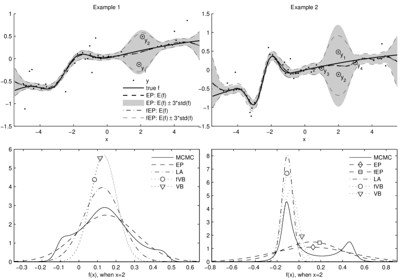
Figure 1 shows two one-dimensional regression problems in which the standard EP may run into problems. In example 1 (the upper left panel) there are two outliers $y_{1}$ and $y_{2}$ providing conflicting information in a region with no regular observations ($1<x<3$). If $\nu$ and $\sigma^{2}$ are sufficiently small, so that the likelihood $p(y_{i}|f_{i})$ is narrow as a function of $f_{i}$, and the length-scale is small inducing small correlation between inputs far apart, there is significant posterior uncertainty about the unknown $f(x)$ when $1<x<3$ and the true posterior is multimodal. The Student-$t$ distribution is able to reject up to $m$ outliers locally, in some neighborhood of an input $\operatorname{\mathbf{x}}$, if there are at least $2m$ observations in that neighborhood. The size of the neighborhood depends on the smoothness properties of the GP prior (governed by the length-scale). In example 1, we have two observations locally which both conflict with $q(f_{1},f_{2}|y_{3},...,y_{n})$ almost equally much and neither one can be labeled as an outlier nor a regular observation. Contrary to the clearly outlying observations for which $\tilde{\tau}_{i}<0$, at convergence the site precisions $\tilde{\tau}_{1}$ and $\tilde{\tau}_{2}$ (corresponding to $y_{1}$ and $y_{2}$) get small positive values, that is, these observations decrease the posterior uncertainty despite being outliers. If the site updates are not damped enough $\tilde{\tau}_{1}$ or $\tilde{\tau}_{2}$ may become negative and cause stability problems.

If the length-scale is sufficiently large in the example 1, the GP prior forces the posterior distribution to become unimodal and both the sequential and the parallel EP converge. This is also the case when the hyperparameters are fixed to their MAP estimates (assuming noninformative priors). The corresponding predictive distribution is visualized in the upper left panel of Figure 1 showing a considerable increase in the posterior uncertainty when $1<x<3$. The lower left panel shows comparison of the predictive distribution of $f(x)$ at $x=2$ obtained with the different approximations described in the section 3. The hyperparameters are estimated separately for each method. The smooth MCMC estimate is calculated by integrating analytically over the latent vector $\operatorname{\mathbf{f}}$ for each posterior draw of the residual variances $\mathbf{V}$ and averaging the resulting Gaussian distributions $q(\tilde{f}|\tilde{x},\mathbf{V},\theta)$. The MCMC estimate (with integration over the hyperparameters) is unimodal but shows small side bumps when the latent function value is close to the observations $y_{1}$ and $y_{2}$. The standard EP estimate (EP1) covers well the posterior uncertainty on the latent value but both the Laplace and fVB underestimate it. At the other input locations where the uncertainty is small, all methods give very similar estimates.

The second one-dimensional regression example, visualized in the upper right panel of Figure 1, is otherwise similar to the example 1 except that the nonlinearity of true function is much stronger when $-5<x<0$, and the observations $y_{1}$ and $y_{2}$ are closer in the input space. The stronger nonlinearity requires a much smaller length-scale for a good data fit and the outliers $y_{1}$ and $y_{2}$ provide more conflicting information (and stronger multimodality) due to the larger prior covariance. The lower right panel shows comparison of the approximative predictive distributions of $f(x)$ when $x=2$. The MCMC estimate has two separate modes near the observations $y_{1}$ and $y_{2}$. The Laplace and fVB approximations are sharply localized at the mode near $y_{1}$ but the standard EP approximation (EP1) is very wide trying to preserve the uncertainty about the both modes. Contrary to the example 1, also the conditional posterior $q(\operatorname{\mathbf{f}}|\operatorname{\mathcal{D}},\theta,\nu,\sigma)$ is two-modal if the hyperparameters are set to their MAP-estimates.

(a) $q(f_{1},f_{2}|y_{3},...,y_{n})$ and $p(y_{1}|f_{1})p(y_{2}|f_{2})$

(b) $q(f_{1},f_{2}|y_{3},...,y_{n})$ $\times p(y_{1}|f_{1})p(y_{2}|f_{2})$

(c) $q(f_{1},f_{2}|y_{3},...,y_{n})$ and $p(y_{1}|f_{1})^{\eta}p(y_{2}|f_{2})^{\eta}$

(d) $q(f_{1},f_{2}|y_{3},...,y_{n})$ $\times p(y_{1}|f_{1})^{\eta}p(y_{2}|f_{2})^{\eta}$

Figure 2: An illustration of a two-dimensional tilted distribution related to the two problematic data points $y_{1}$ and $y_{2}$ in the example 1. Compared to the MAP value used in the Figure 1, shorter lengthscale (0.9) is selected so that the true conditional posterior is multimodal. Panel (a) visualizes the joint likelihood $p(y_{1}|f_{1})p(y_{2}|f_{2})$ together with the approximate marginal $q(f_{1},f_{2}|y_{3},...,y_{n})$ obtained by one round of undamped sequential EP updates on sites $\tilde{t}_{i}(f_{i})$, for $i=3,...,n$. Panel (b) visualizes the corresponding two-dimensional tilted distribution $\hat{p}(f_{1},f_{2})\propto q(f_{1},f_{2}|y_{3},...,y_{n})p(y_{1}|f_{1})p(y_{2}|f_{2})$. Panels (c) and (d) show the same with only a fraction $\eta=0.5$ of the likelihood terms included in the tilted distribution, which corresponds to fractional EP updates on these sites.

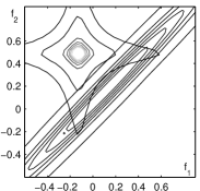
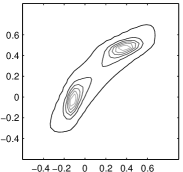
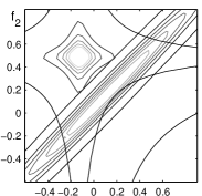
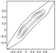
Next we discuss the problems with the standard EP updates with the help of the example 1. Figure 2 illustrates a two-dimensional tilted distribution of the latent values $f_{1}$ and $f_{2}$ related to the observations $y_{1}$ and $y_{2}$ in the example 1. A relatively small lengthscale (0.9) is chosen so that there is large uncertainty on $f_{1}$ and $f_{2}$, but still quite strong prior correlation between them. Suppose that all other sites have already been updated once with the undamped sequential EP starting from a zero initialization ($\tilde{\tau}_{i}=0$ and $\tilde{\nu}_{i}=0$ for $i=1,...,n$). Panel 2(a) visualizes the 2-dimensional marginal approximation $q(f_{1},f_{2}|y_{3},\ldots,y_{n})$ together with the joint likelihood $p(y_{1},y_{2}|f_{1},f_{2})=p(y_{2}|f_{2})p(y_{2}|f_{2})$, and panel 2(b) shows the contours of the resulting two dimensional tilted distribution which has two separate modes. If the site $\tilde{t}_{1}(f_{1})$ is updated next in the sequential manner with no damping, $\tilde{\tau}_{1}$ will get a large positive value and the approximation $q(f_{1},f_{2})$ fits tightly around the mode near the observation $y_{1}$. After this, when the site $\tilde{t}_{2}(f_{2})$ is updated, it gets a large negative precision, $\tilde{\tau}_{2}<0$, since the approximation needs to be expanded toward observation $y_{2}$ which is not at this stage classified as a clear outlier because of the vague prior information. It follows that during the second EP sweep site 1 can no longer be updated because the cavity precision $\tau_{-1}=\sigma_{1}^{-2}-\tilde{\tau_{1}}$ is negative. This happens because there are no other data points supporting the current posterior solution, that is, there are no other sites with positive precision nearby, and the site 2 with negative precision reduces the current marginal precision $\sigma_{1}^{-2}$ too much. If the EP updates were done in parallel, both the cavity and the site precisions would be positive after the first posterior update, but $q(f_{1},f_{2})$ would be tightly centered between the modes. After a couple of parallel loops over all sites, negative cavity variances can emerge as one of the problematic sites gets a too small negative precision because the approximation needs to be expanded to cover all the marginal uncertainty in the tilted distributions.

Skipping updates on the sites with negative cavity variances can keep the algorithm numerically stable (for an example of skipping updates see Minka and Lafferty (2002)), but it is not enough to ensure convergence. In the Figure 2, the large posterior uncertainty about $f_{1}$ and $f_{2}$ requires very small positive precisions $\tilde{\tau}_{i}$ for sites 1 and 2. On the other hand, large differences between the tilted and marginal variances induce large changes on these small site precisions. If the EP updates are not constrained the site parameters may start oscillating between too small and too large values and the algorithm never converges because of too large update steps. One way to reduce the step length is to use damped updates. Decreasing the damping factor $\delta$ sufficiently reduces the oscillations so that the algorithm eventually converges but the convergence can be very slow. Example 2 is more difficult in the sense that convergence requires damping at least with $\delta=0.5$. With the sequential EP the convergence depends also on the update order of the sites and $\delta<0.3$ is needed for convergence with all permutations.

Figures 2(c)–2(d) illustrate the same approximate tilted distribution as Figures 2(a)–2(b) but now only a fraction $\eta=0.5$ of the likelihood terms are included. This corresponds to the first round fractional updates on these sites with zero initialization. Because of the flattened likelihood $p(y_{1}|f_{1})^{\eta}p(y_{2}|f_{2})^{\eta}$ the approximate posterior distribution $q(f_{i},f_{2}|y_{3},...,y_{n})$ is still two-modal but less sharply peaked compared to the standard EP on the left. It follows that also the one-dimensional tilted distributions have smaller variances and the consecutive fractional updates (15) of sites $1$ and $2$ do not widen the marginal variances $\sigma_{1}^{2}$ and $\sigma_{2}^{2}$ as much. The site precisions $\tilde{\tau}_{1}$ and $\tilde{\tau}_{2}$ are larger than with the regular EP and updates on them smaller which requires less damping to keep them positive. This is possible because the different divergence measure allows for a more localized approximation at $1<x<3$. Figure 1 shows a comparison of the standard (EP) and the fractional EP (fEP, $\eta=0.5$) with MAP estimates of the hyperparameters. In the first example both methods produce very similar predictive distribution because the posterior is unimodal. In the second example (lower right panel) the fractional EP gives a much smaller predictive uncertainty estimate when $x=2$ than the standard EP which in turn puts more false posterior mass in the tails when compared to the MCMC.

5.2 Convergence comparisons

Figure 3: A convergence comparison between the sequential and parallel EP as well as the double-loop algorithm in the example 2 (the right panel in Figure 1). For each method both the objective $-\log Z_{EP}$ and the site precisions $\tilde{\tau}_{i}$ related to data points $y_{1},...,y_{4}$ (see Figure 1) are shown. See the text for explanation.

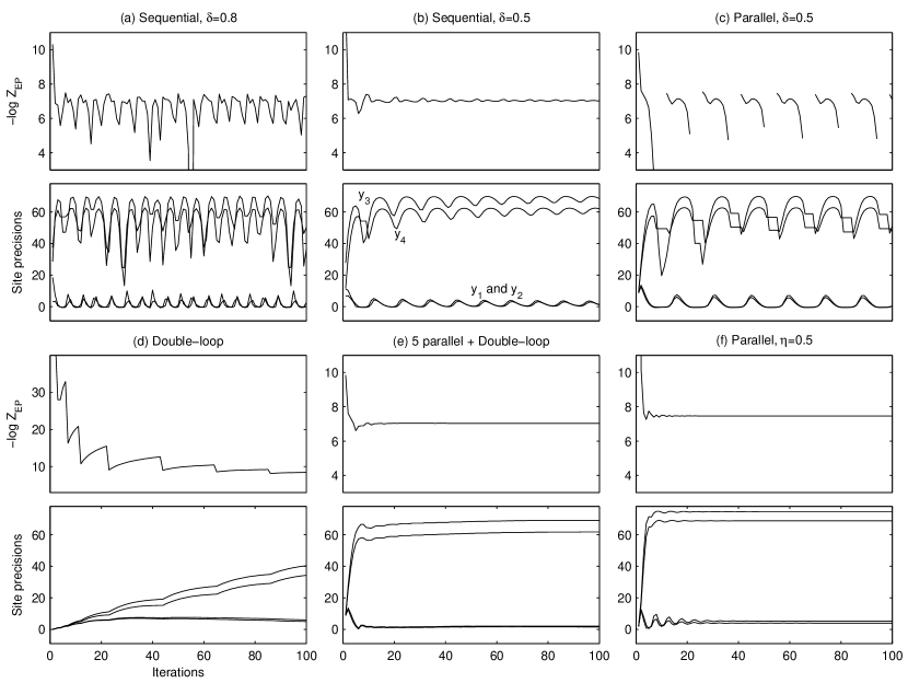
Figure 3 illustrates the convergence properties of the different EP algorithms using the data from the example 2. The hyperparameters were set to: $\nu=2$, $\sigma=0.1$, $\sigma_{se}=3$ and $l_{k}=0.88$. Panel (a) shows the negative marginal likelihood approximation during the first 100 sweeps with the sequential EP and the damping set to $\delta=0.8$. The panel below shows the site precisions corresponding to the observations $y_{1},...,y_{4}$ marked in the upper right panel of Figure 1. With this damping level the site parameters keep oscillating with no convergence and there are also certain parameter values between iterations 50-60 where the marginal likelihood is not defined because of negative cavity precisions (the updates for such sites are skipped until next iteration). Whenever $\tilde{\tau}_{1}$ and $\tilde{\tau}_{2}$ become too small they also inflict large decrease in the nearby sites 3 and 4. These fluctuations affect other sites the more the larger their prior correlations are (defined by the GP prior) with the sites 1 and 2. Panel (b) shows the same graphs with larger amount of damping $\delta=0.5$. Now the oscillations gradually decrease as more iterations are done but convergence is still very slow. Panel (c) shows the corresponding data with the parallel EP and same amount of damping. The algorithm does not converge and the oscillations are much larger compared to the sequential EP. Also the marginal likelihood is not defined at many iterations because of negative cavity precisions.

Panel (d) in Figure 3 illustrates the convergence of the double-loop algorithm with no parallel initialization. There are no oscillations present because the increase of the objective (13) is verified at every iteration and sufficient inner-loop optimality is obtained before proceeding with the outer-loop minimization. However, compared to the sequential or the parallel EP, the convergence is very slow and it takes over 100 iterations to get the site parameters to the level that the sequential EP attains with only a couple of iterations. Panels (e) shows that much faster convergence can be obtained by initializing with 5 parallel iterations and then switching to the double-loop algorithm. There is still some slow drift visible in the site parameters after 20 iterations but changes in the marginal likelihood estimate are very small. Small changes in the site parameters indicate differences in the moment matching conditions (10) and consequently also the gradient of the marginal likelihood estimate may be slightly inaccurate if the implicit derivatives of $\log Z_{EP}$ with respect to $\operatorname{\boldsymbol{\lambda}}_{-}$ and $\operatorname{\boldsymbol{\lambda}}_{s}$ are assumed zero in the gradient evaluations (Opper and Winther, 2005). Panel (f) shows that the parallel EP converges without damping if fractional updates with $\eta=0.5$ are applied. Because of the different divergence measure the posterior approximation is more localized (see Figure 1). It follows that the site precisions related to $y_{1}$ and $y_{2}$ are larger and no damping is required to keep them positive during the updates.

5.3 The marginal likelihood approximation

Figure 4: The approximate log marginal likelihood $\log p(\operatorname{\mathbf{y}}|\operatorname{\mathbf{X}},\theta,\nu,\sigma^{2})$ as a function of the log-length-scale $\log(l_{k}^{2})$ and the log-magnitude $\log(\sigma_{se}^{2})$ in the examples shown in the Figure 1. The marginal likelihood approximation is visualized with both the standard EP ($\eta=1$) and the fractional EP ($\eta=0.5$). The mode of the hyperparameters is marked with $\times$ and $\circ$ for the standard and the fractional EP respectively. For comparison the marginal is also approximated by annealed importance sampling (AIS). For both the standard and the fractional EP the mean absolute errors (MAE) over the region with respect to the AIS estimate are also shown. The noise parameter $\sigma^{2}$ and the degrees of freedom $\nu$ are fixed to the MAP-estimates obtained with $\eta=1$.

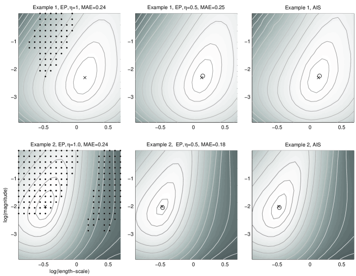
Figure 4 shows contours of the approximate log marginal likelihood with respect to $\log(l_{k})$ and $\log(\sigma^{2}_{se})$ in the examples of Figure 1. The contours in the first column are obtained by applying first the sequential EP with $\delta=0.8$ and using the double-loop algorithm if it does not converge. The hyperparameter values for which the sequential algorithm does not converge are marked with black dots and the maximum marginal likelihood estimate of the hyperparameters is marked with ($\times$). The second column shows the corresponding results obtained with the fractional EP ($\eta=0.5$) and the corresponding hyperparameter estimates are marked with ($\circ$). For comparison, log marginal likelihood estimates determined with the annealed importance sampling (AIS) (Neal, 2001) are shown in the third column.

In the both examples there is an area of problematic EP updates with smaller length-scales which corresponds to the previously discussed ambiguity about the unknown function near data points $y_{1}$ and $y_{2}$ in the Figure 1. There is also a second area of problematic updates at larger length-scale values in example 2. With larger length-scales the model is too stiff and it is unable to explain large proportion of the data points in the strongly nonlinear region ($-4<x<-1$) and consequently there exist no unique unimodal solution. It is clear that with the first artificial example the optimization of the hyperparameters with the sequential EP can fail if not initialized carefully or not enough damping is used. In the second example the sequential EP approximation corresponding to the MAP values cannot even be evaluated because the mode lies in the area of nonconvergent hyperparameter values. In visual comparison with AIS both the standard and fractional EP give very similar and accurate approximations in the first example (the contours are drawn at the same levels for each method). In the second example there are more visible differences: the standard EP tends to overestimate the marginal likelihood due to the larger posterior uncertainties (see Figure 1) whereas fractional EP underestimates it slightly. This is congruent with the properties of the different divergence measure used in the moment matching. The difference between the hyperparameter values at the modes between the standard and fractional EP is otherwise less than 5% except that in the second example $\sigma$ and $\nu$ are ca. 30% larger with the fractional EP.

6 Experiments

Figure 5: A comparison of the approximative predictive means $\operatorname{E}(f_{*}|\operatorname{\mathbf{x}}_{*},\operatorname{\mathcal{D}})$, standard deviations $\text{std}(f_{*}|\operatorname{\mathbf{x}}_{*},\operatorname{\mathcal{D}})$, and probabilities $q(y_{*}|\operatorname{\mathbf{x}}_{*},\operatorname{\mathcal{D}})$ provided by the different approximation methods using 10-fold cross-validation on the Boston housing data. The hyperparameters are fixed to the posterior means obtained by MCMC run on all data. Each dot corresponds to one data point for which the x-coordinate is the MCMC estimate with the fixed hyperparameter values and the y-coordinate the corresponding approximative value obtained with the Laplace’s method (LA), EP, fVB, or VB.

Four data sets are used to compare the approximative methods: 1) An artificial example by Friedman (1991) involving a nonlinear function of 5 inputs. To create a feature selection problem, five irrelevant input variables were added to the data. We generated 10 data sets with 100 training points and 10 randomly selected outliers as described by Kuss (2006). 2) Boston housing data with 506 observations for which the task is to predict the median house prices in the Boston metropolitan area with 13 input variables (see e.g., Kuss, 2006). 3) Data that involves prediction of concrete quality based on 27 input variables for 215 experiments (Vehtari and Lampinen, 2002). 4) Data for which the task is to predict the compressive strength of concrete based on 8 input variables for 1030 observations (Yeh, 1998).

6.1 Predictive comparisons with fixed hyperparameters

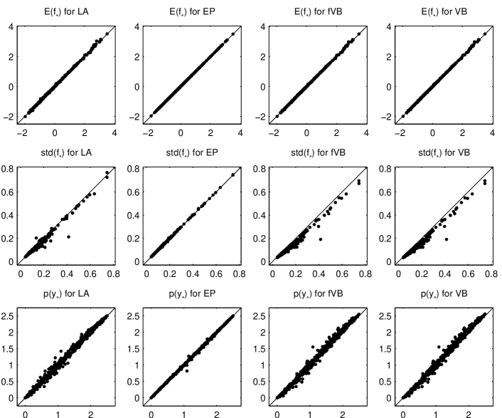
First we compare the quality of the approximate predictive distributions $q(\operatorname{\mathbf{f}}_{*}|\operatorname{\mathbf{x}}_{*},\operatorname{\mathcal{D}},\theta,\nu,\sigma^{2})$, where $x_{*}$ is the prediction location and $f_{*}=f(x_{*})$, between all the approximative methods. We run a full MCMC on the housing data to determine the posterior mean estimates for the hyperparameters. Then the hyperparameters were fixed to these values and a 10-fold cross-validation was done with all the approximations including MCMC. The predictive means and standard deviations of the latent values as well as the predictive densities of the test observations obtained with the Laplace’s method (LA), EP, fVB, and VB are plotted against the MCMC estimate in the Figure 5. Excluding MCMC, the predictive densities were approximated by numerically integrating over the Gaussian approximation of $f_{*}$ in $q(y_{*}|\operatorname{\mathbf{x}}_{*},\operatorname{\mathcal{D}},\theta,\nu,\sigma^{2})=\int p(y_{*}|f_{*},\nu,\sigma^{2})q(f_{*}|\operatorname{\mathbf{x}}_{*},\operatorname{\mathcal{D}},\theta,\nu,\sigma^{2})df_{*}$. EP gives the most accurate estimates for all the predictive statistics, and clear differences to the MCMC can only be seen in the predictive densities which indicates that accurate mean and variance estimates of the latent value may not always be enough when deriving other predictive statistics. This contrast somewhat to the corresponding results in GP classification where Gaussian approximation was shown to be very accurate in estimating predictive probabilities (Nickisch and Rasmussen, 2008). Both fVB and VB approximate the mean well but are overconfident in the sense that they underestimate the standard deviations, overestimate the larger predictive densities, and underestimate smaller predictive densities. LA gives similar mean estimates with the VB approximations but approximates the standard deviations slightly better especially with larger values. Put together, all methods provide decent estimates with fixed hyperparameters but larger performance differences are possible with other hyperparameter values (depending on the non-Gaussianity of the true conditional posterior) and especially when the hyperparameters are optimized.

6.2 Predictive comparisons with estimation of hyperparameter

In this section we compare the predictive performance of LA, EP, fVB, VB, and MCMC with estimation of the hyperparameters. The predictive performance was measured with the mean absolute error (MAE) and the mean log predictive density (MLPD). With the Friedman data these are evaluated using a test set of 1000 latent variables for each of the 10 simulated data sets. For the Boston housing and concrete quality data 10-fold cross validation is used. For the compressive strength data 2-fold cross-validation was used because of the large number observations. To assess the significance of the differences between model performances, 95% credible intervals for the MLPD measures were approximated by Bayesian bootstrap as described by Vehtari and Lampinen (2002). Gaussian likelihood (GA) is selected as a baseline model for comparisons. With GA, LA, EP, and VB the hyperparameters were estimated by optimizing the marginal posterior densities whereas with MCMC all parameters were sampled. The fVB approach was implemented following Kuss (2006) where the hyperparameters are adapted in the M-step of the EM-algorithm. The variational lower bound associated with the M-step was augmented with the same hyperpriors that were used with the other methods.

Since the MAP inference on the degrees of freedom parameter $\nu$ proved challenging due to possible identifiability issues, the LA, EP, fVB, and VB approximations are tested with $\nu$ both fixed to $4$ (LA1, EP1, fVB1, VB1) and optimized together with the other hyperparameters (LA2, EP2, fVB2, VB2). $\nu=4$ was chosen as a robust default alternative to the normal distribution which allows for outliers but still has finite variance compared to the extremely wide-tailed alternatives with $\nu\leq 2$. With EP we also tested a crude but very simple approach (from now on EP3) for improving the robustness of the estimation of $\nu$. We selected 15 values $\nu_{j}$ from the interval $[1.5,20]$ linearly in the log-log scale and ran the optimization of all the other hyperparameters with $\nu$ fixed to these values. The conditional posterior of the latent values was approximated as

$$p(f_{*}|\operatorname{\mathcal{D}},\operatorname{\mathbf{x}})\approx\sum_{j}w_{j}q(\operatorname{\mathbf{f}}|\operatorname{\mathcal{D}},\theta_{j},\sigma_{j}^{2},\nu_{j}),$$

where $\{\theta_{j},\sigma_{j}^{2}\}=\operatorname*{arg\,max}_{\theta,\sigma^{2}}q(\theta,\sigma^{2}|\operatorname{\mathcal{D}},\nu_{j})$ and $w_{j}=q(\theta_{j},\sigma_{j}^{2},\nu_{j}|\operatorname{\mathcal{D}})/\sum_{k}q(\theta_{k},\sigma_{k}^{2},\nu_{k}|\operatorname{\mathcal{D}})$. This can be viewed as a crude approximation of the integration over $\nu$ where $p(\theta,\sigma^{2}|\nu,\operatorname{\mathcal{D}})$ is assumed to be very narrowly distributed around the mode. This approximation requires optimization of $\theta$ and $\sigma^{2}$ with all the preselected values of $\nu$ and to speed up the computations $\theta$ and $\sigma^{2}$ were initialized to the previous mode.

The squared exponential covariance (2) was used for all models. Uniform priors were assumed for $\theta$ and $\sigma^{2}$ on log-scale and for $\nu$ on log-log-scale. The input and target variables were scaled to zero mean and unit variances. The degrees of freedom $\nu$ was initialized to 4, $\sigma$ to 0.5 and the magnitude $\sigma_{se}^{2}$ to 1. The optimization was done with different random initializations for the length-scales $l_{1},...,l_{d}$ and the result with the highest posterior marginal density $q(\theta,\nu,\sigma^{2}|\mathcal{D})$ was chosen. The MCMC inference on the latent values was done with both Gibbs sampling based on the scale-mixture model (3) and direct application of the scaled HMC as described in Vanhatalo and Vehtari (2007). Sampling of the hyperparameters was tested with both slice sampling and HMC. The scale-mixture Gibbs sampling (SM) combined with the slice sampling of the hyperparameters resulted in the best mixing of the chains and gave the best predictive performance and therefore only those results are reported. The convergence and quality of the MCMC runs was checked by both visual inspections as well as by calculating the potential scale reduction factors, effective number of independent samples, and autocorrelation times (Gelman et al., 2004; Geyer, 1992). Based on the convergence diagnostics, burn-in periods were excluded from the beginning of the chains and the remaining draws were thinned to form the final MCMC estimates.

(a) Friedman

(b) Friedman, pairwise

(c) Boston housing

(d) Boston housing, pairwise

(e) Concrete quality

(f) Concrete quality, pairwise

(g) Compressive strength

(h) Compressive strength, pairwise

Figure 6: Left column: The mean log posterior predictive density (MLPD) and its 95% central credible interval. Gaussian observation model (GA) is shown for reference. The Student-$t$ model is inferred with LA, EP, fVB, VB, and scale-mixture based Gibbs sampling (SM). Number 1 after a method means that $\nu$ is fixed, 2 means that it is optimized, and 3 stands for the simple approximative numerical integration over $\nu$. Right column: Pairwise comparisons of the log posterior predictive densities with respect to SM. The mean together with its 95% central credible interval are shown. Values greater than zero indicate that a method is better than SM.

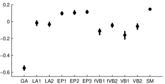
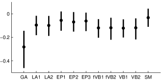
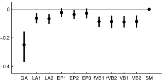
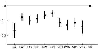
Figures 6(a), 6(c), 6(e) and 6(g) show the MLPD values and their 95% credible intervals for all methods in the four data sets. The Student-$t$ model performs better with all approximations on all data sets compared to the Gaussian model. The differences between the approximations are visible but not very clear. To illustrate the differences more clearly Figures 6(b), 6(d), 6(f) and 6(h) show the pairwise comparisons of the log posterior predictive densities to SM. The mean values of the pairwise differences together with their 95% credible intervals are visualized. The Student-$t$ model with the SM implementation is significantly better than the Gaussian model with higher than 95% probability in all data sets. SM also performs significantly better than all other approximations with the Friedman and compressive strength data and with the Housing data only EP1 is not significantly worse. The differences are much smaller with the concrete quality data and there EP1 performs actually better than SM. One possible explanation for this is a wrong assumption on the noise model (evidence for covariate dependent noise was found in other experiments). Another possibility is the experimental design used in the data collection; there is one input variable that is able to classify large proportion of the observation with very small length scale, and sampling of this parameter may lead to worse performance.

Other pairwise comparisons reveal that either EP1 or EP2 is significantly better than LA, VB, and fVB in all data sets except the compressive strength data for which significant difference is not found when compared to LA1. If the better performing optimization strategy is selected from either LA, fVB, or VB, LA is better than fVB and VB with the Friedman data and the compressive strength data. Between fVB or VB no significant differences were found in pairwise comparisons.

Optimization of $\nu$ proved challenging and sensitive to the initialization of the hyperparameters. The most difficult was fVB for which $\nu$ often drifted slowly towards larger values. This may be due to our implementation that was made following (Kuss, 2006) or more likely to the EM style optimization of the hyperparameters. With LA, EP, and VB the integration over $\operatorname{\mathbf{f}}$ is redone in the inner-loop for all objective evaluations in the hyperparameter optimization, whereas with fVB the optimization is pursued with fixed approximation $q(\operatorname{\mathbf{f}}|\operatorname{\mathcal{D}},\theta,\nu,\sigma^{2})$. The EP-based marginal likelihood estimates were most robust with regards to the hyperparameter initialization. According to pairwise comparisons LA2 was significantly worse than LA1 only in the compressive strength data. EP2 was significantly better than EP1 in the housing and compressive strength data but significantly worse with the housing data. With fVB and VB optimization of $\nu$ gave significantly better performance only with the simulated Friedman data, and significant decrease was observed with VB2 in the housing and compressive strength data. In pairwise comparisons, the crude numerical integration over $\nu$ (EP3) was significantly better than EP1 and EP2 with the housing and compressive strength data, but never significantly worse. These results give evidence that the EP approximation is more reliable in the hyperparameter inference because of the more accurate marginal likelihood estimates which is in line with the results in GP classification (Nickisch and Rasmussen, 2008).

If MAE is considered the Student-$t$ model was significantly better than GA in all other data sets except with the concrete quality data, in which case only EP1 gave better results. If the best performing hyperparameter optimization scheme is selected for each method, EP is significantly better than the others with all data sets except with the compressive strength data in which case the differences were not significant. When compared to SM, EP was better with the Friedman and concrete quality data, otherwise no significant differences were found. LA was significantly better than fVB and VB in the compressive strength data whereas with the simulated Friedman data VB was better than LA and fVB.

Table 1: Two upper rows: The relative CPU times required for the hyperparameter inference. The times are scaled to yield 1 for LA1 separately for each of the four data sets, and both the relative mean (mean) as well as the maximum (max) over the data sets are reported. The third row: The average relative CPU times over the four data sets with the hyperparameters fixed to 28 preselected configurations.

	GA	LA1	LA2	EP1	EP2	EP3	fVB1	fVB2	VB1	VB2	SM
mean	0.07	1.0	0.8	0.8	7.0	13	15	8.9	1.6	1.8	280
max	0.09	1.0	1.2	1.1	16	26	39	22	3.3	3.8	440
fixed	0.1	1.0		5.5			2.4		1.9		–

Table 1 summarizes the total CPU times required for the posterior inference (includes hyperparameter optimization and the predictions). The CPU times are scaled to give one for LA1 and both the mean and maximum over the four data sets are reported. The running times for the fastest Student-$t$ approximations are roughly 10-fold compared to the baseline method GA. EP1, where $\nu=4$, is surprisingly fast compared to the LA but with the optimization of $\nu$ (EP2) it gets much slower. This is explained by the increasing number of double-loop iterations required to achieve convergence with the larger number of difficult posterior distributions as $\nu$ gets smaller values. The EP3 is clearly more demanding compared to EP1 or EP2 because the optimization has to be repeated with every preselected value of $\nu$. The fVB is quite slow compared to LA or VB because of the slowly progressing EM-based hyperparameter adaptation. With the LA and VB the running times are quite similar with $\nu$ both fixed and optimized. The running times are suggestive in the sense that they depend much on the implementations, convergence thresholds and initial guess of the hyperparameters. Table 1 shows also the average relative running times over the four data sets (excluding MCMC) with the hyperparameters fixed to 28 different configurations (fixed). The configurations were created by first including the MCMC mean for each data set and then generating all combinations of three clearly different values of $\nu$, $\sigma$, and $\sigma_{se}$ around the MCMC mean with randomly selected lengthscales. Quite many difficult hyperparameter configurations were created which shows in the larger running time with the EP.

7 Discussion

Much research has been done on the EP and it has been found very accurate and computationally efficient in many practical applications. Non-log-concave site functions may be problematic for the EP but it has been utilized and found effective for many potentially difficult models such as the Gaussian mixture likelihoods (Kuss, 2006; Stegle et al., 2008) and priors (spike and slab, Hernández-Lobato et al., 2008). Modifications such as the damping and the fractional updates as well as alternative double-loop algorithms have been proposed to improve the stability in difficult cases but the practical implementation issues have not been discussed that much. In this work we have given an example of the good predictive performance of the EP in a challenging model but also analyzed the convergence problems and the proposed improvements from a practical point of view. The Student-$t$ model is an interesting example because it gives a natural interpretation for the negative site precisions as the increase of the posterior uncertainty related to the not-so-clear outliers. On the other hand, conflicting outliers in a region with considerable uncertainty about the unknown function values may require very small but positive site precisions, which turned out to be problematic for the regular EP updates in our experiments.

The nonlinear GP regression makes the inference problem even more challenging because the multimodality of the conditional posterior depends on the hyperparameter values. In practical applications, when the hyperparameters are optimized, an estimate of the marginal likelihood is important also with the more difficult cases. As we have demonstrated by examples, standard EP, unless damped sufficiently, may not converge with the maximum marginal likelihood estimate of the hyperparameters, and therefore, one cannot simply discard these hyperparameter values. In our examples these situations were related to two modes in the conditional posterior (caused by two outliers) quite far away from each other which requires a very large local increase of marginal variance from the unimodal posterior approximation. (It should also be noted that moderately damped sequential EP worked fine with many other multimodal posterior distributions.) The globally unimodal assumption is not the best in such cases although the true underlying function is unimodal, but we think that it is important to get some kind of posterior approximation. Whether one prefers the possible false certainty provided by the Laplace or VB approximations, or the possible false uncertainty of the EP, is a matter of taste but we prefer the latter one.

It is also important that the inference procedure gives some clue of the underlying problems so that more elaborate models can be designed. In addition to the examination of the posterior approximation, the need for double-loop iterations in our EP implementation may be one indication of an unsuitable model. One can also compare the cavity distributions which can be regarded as LOO estimates of the latent values. If for certain sites most of the LOO information comes from the corresponding site approximations, i.e., the cavity precisions are close to zero, there is reason to suspect that the approximation is not suitable. Our EP implementation enables a robust way of approaching this limit and in case of problems one can switch to fractional updates.

In this work we have focused on the Student-$t$ model and have omitted comparisons to other robust observations models such as the Laplace distribution and mixtures of Gaussians (Kuss, 2006; Stegle et al., 2008). Laplace distribution and Gaussian mixtures are computationally convenient since the moment evaluations required for the EP updates can be done analytically. However, the Student-$t$ model is more general in the sense that it can be thought of as an infinite mixture of Gaussians and parameter $\nu$ can be used to continuously adjust the degree of robustness. In addition, it contains the Gaussian distribution as a special case. The thickness of the tails could be adjusted also with a finite mixture of Gaussians but the number of parameters increases with the number of mixture components. Inferring a point estimate of $\nu$ from the data turned out to be challenging but EP was the most consistent approximative method for it in our experiments. We showed that fixing $\nu=4$ gives a good baseline model for comparisons and we also described a simple grid based approximation for improving the estimation of $\nu$ based on data. The presented modifications for improving the robustness of the parallel EP are general and they could be applied also for other non-log-concave likelihoods. The presented EP approach for GP regression with a Student-$t$ likelihood will be implemented in the freely available GPstuff software package (http://www.lce.hut.fi/research/mm/gpstuff/).

References

- Bishop (2006) Christopher M. Bishop. Pattern Recognition and Machine Learning. Springer, 2006.
- Cseke and Heskes (2011) Botond Cseke and Tom Heskes. Properties of Bethe free energies and message passing in Gaussian models. Journal of Artificial Intelligence Research, 2011.
- Dawid (1973) A. Philip Dawid. Posterior expectations for large observations. Biometrika, 60(3):664–667, December 1973.
- De Finetti (1961) Bruno De Finetti. The Bayesian approach to the rejection of outliers. In Proceedings of the fourth Berkeley Symposium on Mathematical Statistics and Probability, pages 199–210. University of California Press, 1961.
- Friedman (1991) Jerome H. Friedman. Multivariate adaptive regression splines. Annals of Statistics, 19(1):1–67, 1991.
- Gelman et al. (2004) Andrew Gelman, John B. Carlin, Hal S. Stern, and Donald B. Rubin. Bayesian Data Analysis. Chapman & Hall/CRC, second edition, 2004.
- Geweke (1993) John Geweke. Bayesian treatment of the independent Student- linear model. Journal of Applied Econometrics, 8:519–540, 1993.
- Geyer (1992) C. J. Geyer. Practical Markov chain Monte Carlo. Statistical Science, 7(12):473–483, 1992.
- Gibbs and MacKay (2000) Mark N. Gibbs and David J. C. MacKay. Variational Gaussian process classifiers. In IEEE Transactions on Neural Networks, pages 1458–1464, 2000.
- Goldberg et al. (1998) Paul W. Goldberg, Christopher K.I. Williams, and Christopher M. Bishop. Regression with input-dependent noise: A Gaussian process treatment. In M. I. Jordan, M. J. Kearns, and S. A Solla, editors, Advances in Neural Information Processing Systems 10. MIT Press, Cambridge, MA, 1998.
- Hernández-Lobato et al. (2008) José Miguel Hernández-Lobato, Tjeerd Dijkstra, and Tom Heskes. Regulator discovery from gene expression time series of malaria parasites: a hierarchical approach. In J.C. Platt, D. Koller, Y. Singer, and S. Roweis, editors, Advances in Neural Information Processing Systems 20, pages 649–656, Cambridge, MA, 2008. MIT Press.
- Heskes and Zoeter (2002) Tom Heskes and Onno Zoeter. Expectation propagation for approximate inference in dynamic Bayesian networks. In A. Darwiche and N. Friedman, editors, Uncertainty in Artificial Intelligence: Proceedings of the Eighteenth Conference (UAI-2002), pages 216–233, San Francisco, CA, 2002. Morgan Kaufmann Publishers.
- Heskes et al. (2005) Tom Heskes, Manfred Opper, Wim Wiegerinck, Ole Winther, and Onno Zoeter. Approximate inference techniques with expectation constraints. Journal of Statistical Mechanics: Theory and Experiment, 2005:P11015, 2005.
- Kuss (2006) Malte Kuss. Gaussian Process Models for Robust Regression, Classification, and Reinforcement Learning. PhD thesis, Technische Universität Darmstadt, 2006.
- Minka (2001a) Thomas Minka. Expectation propagation for approximate Bayesian inference. In UAI ’01: Proceedings of the 17th Conference in Uncertainty in Artificial Intelligence, pages 362–369, San Francisco, CA, USA, 2001a. Morgan Kaufmann Publishers Inc.
- Minka (2001b) Thomas Minka. A Family of Algorithms for Approximate Bayesian Inference. PhD thesis, Massachusetts Institute of Technology, 2001b.
- Minka (2004) Thomas Minka. Power EP. Technical report, Microsoft Research, Cambridge, 2004.
- Minka (2005) Thomas Minka. Divergence measures and message passing. Technical report, Microsoft Research, Cambridge, 2005.
- Minka and Lafferty (2002) Thomas Minka and John Lafferty. Expectation-propagation for the generative aspect model. In Proceedings of the 18th Conference on Uncertainty in Artificial Intelligence, pages 352–359. Morgan Kaufmann, 2002.
- Naish-Guzman and Holden (2008) Andrew Naish-Guzman and Sean Holden. Robust regression with twinned Gaussian processes. In J.C. Platt, D. Koller, Y. Singer, and S. Roweis, editors, Advances in Neural Information Processing Systems 20, pages 1065–1072. MIT Press, Cambridge, MA, 2008.
- Neal (1997) Radford M. Neal. Monte Carlo Implementation of Gaussian Process Models for Bayesian Regression and Classification. Technical Report 9702, Dept. of statistics and Dept. of Computer Science, University of Toronto, January 1997.
- Neal (2001) Radford M. Neal. Annealed importance sampling. Statistics and Computing, 11:125–139, 2001.
- Nickisch and Rasmussen (2008) Hannes Nickisch and Carl Edward Rasmussen. Approximations for binary Gaussian process classification. Journal of Machine Learning Research, 9:2035–2078, October 2008.
- O’Hagan (1979) Anthony O’Hagan. On outlier rejection phenomena in Bayes inference. Journal of the Royal Statistical Society. Series B., 41(3):358–367, 1979.
- Opper and Archambeau (2009) Manfred Opper and Cédric Archambeau. The variational Gaussian approximation revisited. Neural Computation, 21(3):786–792, March 2009.
- Opper and Winther (2005) Manfred Opper and Ole Winther. Expectation Consistent Approximate Inference. J. Mach. Learn. Res., 6:2177–2204, December 2005.
- Rasmussen and Nickisch (2010) C. E. Rasmussen and H. Nickisch. Gaussian processes for machine learning (GPML) toolbox. Journal of Machine Learning Research, 11:3011–3015, 2010.
- Rasmussen and Williams (2006) Carl Edward Rasmussen and Christopher K. I. Williams. Gaussian Processes for Machine Learning. The MIT Press, 2006.
- Rue et al. (2009) Håvard Rue, Sara Martino, and Nicolas Chopin. Approximate Bayesian inference for latent Gaussian models by using integrated nested Laplace approximations. Journal of the Royal statistical Society B, 71(2):1–35, 2009.
- Seeger and Nickisch (2011) M. Seeger and H. Nickisch. Fast convergent algorithms for expectation propagation approximate Bayesian inference. Artificial Intelligence and Statistics 14, 2011.
- Seeger (2005) Matthias Seeger. Expectation propagation for exponential families. Technical report, Max Planck Institute for Biological Cybernetics, Tübingen, Germany, 2005.
- Seeger (2008) Matthias Seeger. Bayesian inference and optimal design for the sparse linear model. Journal of Machine Learning Research, 9:759–813, 2008.
- Shampine (2008) Lawrence F. Shampine. Vectorized adaptive quadrature in MATLAB. Journal of Computational and Applied Mathematics, 211:131–140, February 2008.
- Stegle et al. (2008) Oliver Stegle, Sebastian V. Fallert, David J. C. MacKay, and Søren Brage. Gaussian process robust regression for noisy heart rate data. Biomedical Engineering, IEEE Transactions on, 55(9):2143–2151, September 2008.
- Tierney and Kadane (1986) Luke Tierney and Joseph B. Kadane. Accurate approximations for posterior moments and marginal densities. Journal of the American Statistical Association, 81(393):82–86, 1986.
- Tipping and Lawrence (2003) M E Tipping and N D Lawrence. A variational approach to robust Bayesian interpolation. In In Proceedings of the IEEE International Workshop on Neural Networks for Signal Processing, pages 229–238. IEEE, 2003.
- Tipping and Lawrence (2005) Michael E. Tipping and Neil D. Lawrence. Variational inference for Student- models: Robust bayesian interpolation and generalised component analysis. Neurocomputing, 69:123–141, 2005.
- van Gerven et al. (2009) Marcel van Gerven, Botond Cseke, Robert Oostenveld, and Tom Heskes. Bayesian source localization with the multivariate Laplace prior. In Y. Bengio, D. Schuurmans, J. Lafferty, C. K. I. Williams, and A. Culotta, editors, Advances in Neural Information Processing Systems 22, pages 1901–1909, 2009.
- Vanhatalo and Vehtari (2007) Jarno Vanhatalo and Aki Vehtari. Sparse log Gaussian processes via MCMC for spatial epidemiology. JMLR Workshop and Conference Proceedings, 1:73–89, 2007.
- Vanhatalo et al. (2009) Jarno Vanhatalo, Pasi Jylänki, and Aki Vehtari. Gaussian process regression with Student- likelihood. In Y. Bengio, D. Schuurmans, J. Lafferty, C. K. I. Williams, and A. Culotta, editors, Advances in Neural Information Processing Systems 22, pages 1910–1918. 2009.
- Vehtari and Lampinen (2002) Aki Vehtari and Jouko Lampinen. Bayesian model assessment and comparison using cross-validation predictive densities. Neural Computation, 14(10):2439–2468, 2002.
- West (1984) Mike West. Outlier models and prior distributions in Bayesian linear regression. Journal of the Royal Statistical Society. Series B., 46(3):431–439, 1984.
- Williams and Barber (1998) Christopher K. I. Williams and David Barber. Bayesian classification with Gaussian processes. IEEE Transactions on Pattern Analysis and Machine Intelligence, 20(12):1342–1351, 1998.
- Yeh (1998) I-Cheng Yeh. Modeling of strength of high performance concrete using artificial neural networks. Cement and Concrete Research, 28(12):1797–1808, 1998.