The accuracy of stellar atmospheric parameter determinations: a case study with HD 32115 and HD 37594

Abstract

We present detailed parameter determinations of two chemically normal late A-type stars, HD 32115 and HD 37594, to uncover the reasons behind large discrepancies between two previous analyses of these stars performed with a semi-automatic procedure and a “classical” analysis. Our study is based on high resolution, high signal-to-noise spectra obtained at the McDonald Observatory. Our method is based on the simultaneous use of all available observables: multicolor photometry, pressure-sensitive magnesium lines, metallic lines and Balmer line profiles. Our final set of fundamental parameters fits, within the error bars, all available observables. It differs from the published results obtained with a semi-automatic procedure. A direct comparison between our new observational material and the spectra previously used by other authors shows that the quality of the data is not the origin of the discrepancies. As the two stars require a substantial macroturbulence velocity to fit the line profiles, we concluded that neglecting this additional broadening in the semi-automatic analysis is one origin of discrepancy. The use of Fe i excitation equilibrium and of the Fe ionisation equilibrium, to derive effective temperature and surface gravity, respectively, neglecting all other indicators leads to a systematically erroneously high $T_{\mathrm{eff}}$. We deduce that the results obtained using only one parameter indicator might be biased and that those results need to be cautiously taken when performing further detailed analyses, such as modelling of the asteroseismic frequencies or characterising transiting exoplanets.

1 Introduction

The advent of space missions aiming to obtain very accurate photometry for an increasing number of stars (e.g. CoRoT and Kepler) led to the necessity of a large scale work to obtain high precision spectroscopic fundamental parameters, effective temperature in particular, to allow i.e. the modelling of the pulsation frequencies or the characterisation of transiting exoplanets. This large spectroscopic analysis campaign can be performed within reasonable time-scales only with automatic and semi-automatic procedures. It is therefore crucial to critically compare some of the results obtained in this way with other independent, more “classical”, methods and highlight the discrepancies to understand their origin and improve these procedures.

Bruntt et al. (2010) derived fundamental parameters for a set of 23 solar-type stars adopting various different techniques (e.g. asteroseismology, parallax, spectroscopy), concluding that purely spectroscopic methods lead to results comparable to the more robust ones, although small corrections might be necessary. It is important to carefully assess whether there are cases where the spectroscopy fails in recovering the correct set of parameters, and if such erroneous parameters are produced, we need to understand why and correct the methodology.

In this work we concentrate on a few discordant results obtained with the semi-automatic procedure developed by H. Bruntt (see e.g. Bruntt et al. 2002) and adopted by many authors to analyse several different types of stars.

For the solar-type pulsator HD 49933, Gillon & Magain (2006) and Bruntt et al. (2008) (hereafter B08), making use of two very similar semi-automatic procedures, derived an effective temperature ($T_{\mathrm{eff}}$) of about 6750 K. Ryabchikova et al. (2009, hereafter R09) re-analysed this same star applying a “classical” analysis (based on photometry, equivalent widths and hydrogen lines) to higher quality spectra, obtaining a $T_{\mathrm{eff}}$ of 6500 K, demonstrating this is a better value for $T_{\mathrm{eff}}$. Later Bruntt (2009) reanalysed the same spectra of HD 49933 used by R09 with the same method used by B08 obtaining a $T_{\mathrm{eff}}$ of 6570 K, in agreement with R09, but in disagreement with B08. The later analysis did not explain the reason for such disparate results from the same semi-automatic procedure on the same star, leaving open the possibility that different results might be obtained with data from different instruments. This possibility needs to be ruled out and it is important to understand the origin of these discrepancies, furthermore because the code employed by B08 and Bruntt (2009) is adopted for most of the spectroscopic analysis of the CoRoT stars.

To understand the discrepancies, we must examine more than one star, therefore we decided to extend our critical analysis of B08’s methodology for fundamental parameter determination to two other stars: HD 32115 and HD 37594, used as comparison stars by B08. Bikmaev et al. (2002) showed the results of a fundamental parameter determination and abundance analysis of these two stars performed with a classical method, obtaining $T_{\mathrm{eff}}$ of 7250 K and 7170 K, respectively. B08 re-analysed HD 32115 and HD 37594 employing a semi-automatic procedure on a different set of spectra, obtaining 7670 K and 7380 K, respectively. Here we use higher quality data than that previously used by Bikmaev et al. (2002) and B08, focusing on the parameter determination and using only carefully selected spectral lines considering their $\log{gf}$ values, blending, and known non-LTE effects affecting those lines.

HD 32115 is a single line spectroscopic binary for which Fekel et al. (2006) determined an orbital period of about 8 days, and concluded that the companion is either a late K- or an early M-type star. This ensures that the spectral lines of the primary are not affected by the companion at any wavelength and that it is also safe to perform a spectrophotometric analysis to derive the stellar parameters of the primary star (see Sect. 4.1.2).

For HD 32115, Fekel et al. (2006) derived an effective temperature of 7251 K and a surface gravity of 4.26. From the HIPPARCOS parallax and from their orbit analysis, Fekel et al. (2006) derived a stellar mass and radius of 1.5 $M/M_{\odot}$ and 1.5$\pm$0.1 $R/R_{\odot}$, respectively. By means of stellar structure and evolution calculations, Allende Prieto & Lambert (1999) derived an effective temperature of 7413 K and a surface gravity of 4.29$\pm$0.04. They derived also a stellar mass of 1.54$\pm$0.06 $M/M_{\odot}$ and a stellar radius of 1.48$\pm$0.03 $R/R_{\odot}$. We notice that Bikmaev et al. (2002)’s $T_{\mathrm{eff}}$ for HD 32115 coincides with the effective temperatures obtained by Fekel et al. (2006). On the other hand, B08’s $T_{\mathrm{eff}}$ does not agree with any of the previous determinations.

2 Observations

Spectra of HD 32115 and of HD 37594 were obtained on 2010, November 30th with the Robert G. Tull Coudé Spectrograph (TS) attached at the 2.7-m telescope of McDonald Observatory. This is a cross-dispersed échelle spectrograph yielding a resolving power ($R$) of 60 000 for the configuration used here. The signal-to-noise ratio (S/N) per pixel at $\lambda\sim$5000 Å is 490 and 535, respectively for HD 32115 and HD 37594.

Bias and flat-field frames were obtained at the beginning of the night, and a Th-Ar spectrum, for wavelength calibration, was obtained between the two science spectra, which were reduced using the Image Reduction and Analysis Facility (IRAF, Tody 1993). Each spectrum, normalised by fitting a low order polynome to carefully selected continuum points, covers the wavelength range 3633–10849 Å, with several gaps between the orders at wavelengths greater than 5880 Å. Making use of the Th-Ar spectrum we ensured the stability of the resolution. The CCD count rates were well below the saturation level, ensuring linearity and therefore no systematic differences between strong and weak lines. This was also confirmed by the complete absence of any correlation between line abundance and wavelength (see Sect.3.2.3).

The normalisation of the H$\gamma$ line was of crucial importance since we adopted the profile fitting of the H$\gamma$ line wings as one of the temperature indicators. We were unable to use either H$\alpha$ and H$\beta$ because the former was not covered by our spectra and the latter was affected by a spectrograph defect, preventing the normalisation. We were able to perform a reliable normalisation of the H$\gamma$ line using the artificial flat-fielding technique described by Barklem et al. (2002). This normalisation procedure was already successfully applied to data obtained with this spectrograph by Kolenberg et al. (2010).

2.1 Comparing spectrographs

As mentioned in Sect. 1, Bruntt (2009) left open the possibility that the discrepancies obtained for HD 49933 with their previous results (B08) were caused by systematic differences in the observed spectra (Bruntt 2009, analysed HARPS spectra, while B08 analysed CORALIE spectra, where both instruments operate at LaSilla, but on different telescopes). We checked if this is the case. This control is important, to remove the observed spectra as a possible source of systematic uncertainties and also to check the quality of the normalisation, as independently performed on spectra obtained with different instruments.

Here we compare the spectra obtained with TS and CORALIE (used by B08), which is an échelle spectrograph, reaching a resolution of $R\sim$50 000, mounted on the 1.2-m Euler telescope in La Silla, Chile. Details of the CORALIE spectrograph and on the data reduction can be found in De Cat et al. (2006).

Figure 1 shows a comparison between the TS and the CORALIE spectrum of HD 32115 in the wavelength range around the strong Fe ii $\lambda$5018 Å line. In this plot we display also the difference spectrum (in % shifted upwards of 0.9) between the two spectra.

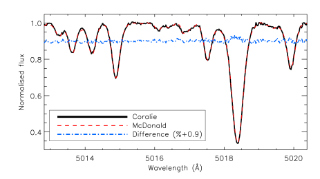
Figure 1: Comparison between the spectra of HD 32115 obtained with the CORALIE spectrograph (dashed red line) and the TS spectrograph (thick black line) in the wavelength region around the $\lambda$5018 Å Fe ii line. The difference (in %) between the two spectra is shown by the dashed- dotted blue line. The difference spectrum is shifted upwards by 0.9. No difference is visible between the two spectra, except for the core of the strong Fe ii line at $\lambda$5018 Å which displays the difference in resolution between the two instruments.

The rms of the difference spectrum (a portion is shown in Fig. 1), calculated on several continuum regions is comparable to the rms of the CORALIE spectrum. We obtained the same conclusion comparing the TS and CORALIE spectra with the ones used by Bikmaev et al. (2002). The spectra of HD 37594 demonstrate an identical behavior.

These comparisons let us conclude that there are no significant differences between the spectra used in the present work and those employed by Bikmaev et al. (2002) and by B08, thus excluding the quality of the data as the origin of the discrepancies described in Sect. 1. In addition, this comparison sets an upper limit of $\sim$1% on the uncertainty due to the normalisation.

3 The fundamental parameters

We adopted photometric indicators to set the starting point in the determination of the fundamental parameters, which we refined making use of hydrogen lines, metal lines, and, as a final check, synthetic colors and the spectral energy distribution. Spectroscopic tuning of the fundamental parameters is needed because different photometric systems and calibrations give different parameters and uncertainties. Spectroscopic analysis, performed with in this way, will produce a parameter set which fits all the indicators consistently, the uncertainties are thus reduced for those derived from photometric analysis alone.

We computed model atmospheres of HD 32115 and HD 37594 using the LLmodels stellar model atmosphere code (Shulyak et al. 2004). For all the calculations Local Thermodynamical Equilibrium (LTE) and plane-parallel geometry were assumed. We used the VALD database (Piskunov et al. 1995; Kupka et al. 1999; Ryabchikova et al. 1999) as a source of atomic line parameters for opacity calculations. Convection was implemented according to the Canuto & Mazzitelli (1991, 1992) model of convection (see Heiter et al. 2002, for more details).

3.1 Photometric indicators

Initial guesses for the effective temperature ($T_{\mathrm{eff}}$) and surface gravity ($\log g$) were obtained from calibrations of different photometric indices for normal stars. The effective temperature and gravity were derived from Strömgren photometry (Hauck & Mermilliod 1998) with calibrations by Moon & Dworetsky (1985), Napiwotzki et al. (1993), Balona (1994), Ribas et al. (1997), Castelli et al. (1997), and from Geneva photometry (Rufener 1988) with calibrations by North & Nicolet (1990).

Table 1 summarises the set of $T_{\mathrm{eff}}$ and $\log g$ obtained with each adopted calibration and photometry, reflecting the scattering due to the use of different calibrations and photometric systems.

Table 1: Set of $T_{\mathrm{eff}}$ and $\log g$ obtained for HD 32115 and HD 37594 using different calibrations for Strömgren (Hauck & Mermilliod 1998) and Geneva (Rufener 1988) photometry. The last two lines give the average values of $T_{\mathrm{eff}}$ and $\log g$, with their uncertainties, calculated without taking into account the results from the Castelli et al. (1997) calibration.

	HD 32115		HD 37594
Photometry	$T_{\mathrm{eff}}$ [K]	$\log g$	$T_{\mathrm{eff}}$ [K]	$\log g$	Calibration
Strömgren	7296	4.23	7171	4.22	Moon & Dworetsky (1985)
	7207	4.13	6899	3.86	Napiwotzki et al. (1993)
	7421	4.11	7276	4.05	Balona (1994)
	7308	4.27	7189	4.32	Ribas et al. (1997)
	6998	3.84	6667	3.47	Castelli et al. (1997)
Geneva	7263	4.47	7157	4.47	North & Nicolet (1990)
	7300$\pm$80	4.24$\pm$0.14	7140$\pm$142	4.18$\pm$0.24

The interstellar reddening plays an important role when converting the observed photometry into fundamental parameters. We calculated the interstellar reddening adopting the galactic extinction maps provided by Amôres & Lépine (2005), obtaining E($B-V$)=0.00 for both stars, which we adopt for the determination of the synthetic colors (see Sect. 4.1.1) and spectral energy distribution (see Sect. 4.1.2). This is also in agreement with other models of interstellar extinction in the solar neighborhood, e.g. Lallement et al. (2003).

Excluding the results obtained with the calibration by Castelli et al. (1997), which gives much lower $T_{\mathrm{eff}}$ and $\log g$ compared to the others, we set the center for the calculation of our model grid to $T_{\mathrm{eff}}$ = 7250 K and $\log g$ = 4.2, for HD 32115 and to $T_{\mathrm{eff}}$ = 7100 K and $\log g$ = 4.2, for HD 37594, adopting steps of 50 K in $T_{\mathrm{eff}}$ and 0.1 in $\log g$.

3.2 Spectroscopic indicators

3.2.1 Hydrogen lines

For a fully consistent abundance analysis, the photometric parameters must be checked and eventually tuned according to spectroscopic indicators, such as hydrogen line profiles. In the temperature range where HD 32115 and HD 37594 lie, the hydrogen line wings are sensitive almost exclusively to $T_{\mathrm{eff}}$ variations. To spectroscopically derive $T_{\mathrm{eff}}$ from hydrogen lines, we fitted synthetic line profiles, calculated with SYNTH3 (Kochukhov 2007), to the observed H$\gamma$ profiles. SYNTH3 incorporates the code by Barklem et al. (2000) that takes into account not only self-broadening but also Stark broadening (see their Sect. 3). For the latter, the default mode of SYNTH3, adopted in this work, uses an improved and extended HLINOP routine (Kurucz 1993).

Figure 2 shows a comparison of the observed H$\gamma$ line profiles of HD 32115 and HD 37594, with two synthetic profiles for each star. One synthetic profile was calculated with our final set of parameters while the other one with the set of parameters by B08.

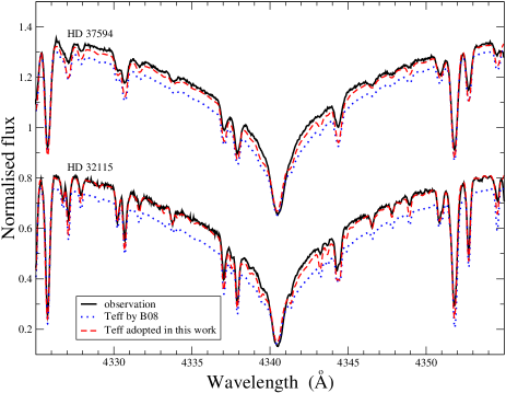
Figure 2: Comparison between the observed H$\gamma$ line profile (black solid line) and synthetic profiles calculated with our final adopted parameters (red dashed line) and with the parameters adopted by B08 (blue dotted line). The upper comparison is for HD 37594, while the lower comparison is for HD 32115. Our final adopted set of parameters is $T_{\mathrm{eff}}$ = 7250$\pm$100 K, $\log g$ = 4.2$\pm$0.1 for HD 32115 and $T_{\mathrm{eff}}$ = 7150$\pm$100 K, $\log g$ = 4.2$\pm$0.1 for HD 37594. B08’s set of parameters is $T_{\mathrm{eff}}$ = 7670$\pm$170 K, $\log g$ = 4.44$\pm$0.13 for HD 32115 and $T_{\mathrm{eff}}$ = 7380$\pm$190 K, $\log g$ = 4.08$\pm$0.16 for HD 37594. The profiles shown for HD 37594 were rigidly shifted upwards by 0.5.

For both stars, the synthetic spectrum corresponding to our final model (see Sect. 4) does not fit the H$\gamma$ profile perfectly, this would require a lower temperature by $\sim$80–100 K. We attribute most of the difference between our final synthetic and observed H$\gamma$ profiles to the normalisation, which is always challenging for hydrogen lines observed with échelle spectra. To quantify the uncertainty introduced by the normalisation, we compared the TS H$\gamma$ profile with the one we obtained from the CORALIE spectrum. The maximum difference between the two profiles (independently normalised) is $\sim$2%, less than the difference introduced in the synthetic spectrum by changing $T_{\mathrm{eff}}$ by 100 K.

Figure 2 shows that the effective temperatures adopted by B08 for the two stars are too high to even remotely fit the hydrogen line profiles.

3.2.2 Gravity from metallic lines with extended wings

The surface gravity was derived from two independent methods based on line profile fitting of Mg i lines with developed wings (analysis described here) and ionisation balance for several elements (analysis performed in Sect. 3.2.3). The first method is described in Fuhrmann et al. (1997) and is based on the fact that the wings of the Mg i lines at $\lambda\lambda$ 5167, 5172 and 5183 Å are very sensitive to $\log g$ variations. In practice, first the Mg abundance is determined from other Mg i lines without developed wings, such as $\lambda$ 5528 Å, and then the wings of the three lines listed above are tuned to the $\log g$ value.

It was not possible to use the Mg i lines at $\lambda\lambda$ 5167 and 5183 Å because the former is blended by a strong Fe i line, while the latter falls at the border of two overlapping spectral orders and the normalisation was not good enough for the required precise fitting of the line wings. In the end, we based our fit for the $\log g$ determination just on the Mg i line at $\lambda$ 5172 Å.

For HD 32115, we used the Mg i line at $\lambda$ 5528 Å and the Mg ii line at $\lambda$ 7877 Å to measure the Mg abundance, while for HD 37594 we used only the former because the latter is blended with a telluric line, making the abundance determination unreliable.

Given the presence of non-LTE effects for Mg, in particular for the Mg ii infrared line (Abia & Mashonkina 2004), we calculated the non-LTE corrections for the Mg lines used. As our synthetic line profiles are in LTE, non-LTE calculations are necessary to make sure that the Mg abundance, we derive from the Mg i $\lambda$ 5528 Å and Mg ii $\lambda$ 7877 Å lines, is correct and therefore applicable for the line profile fitting of the Mg i $\lambda$ 5172 Å line.

Non-LTE corrections for neutral and singly-ionised magnesium were carried out using the codes DETAIL and SURFACE, originally developed by Giddings (1981) and Butler (1984) along with the model atmosphere computed with LLmodels. Our calculations take into account the recent improvements in the atomic data for Mg, the extensive description of the model atom, and non-LTE line formation presented by Przybilla et al. (2001). For both stars the non-LTE abundance correction $\Delta(Mg/N_{tot})=\log(Mg/N_{tot})^{LTE}-\log(Mg/N_{tot})^{NLTE}$ is $+0.02$ dex for the Mg i lines at $\lambda$ 5172 and 5528 Å, while for the Mg ii infrared line at $\lambda$ 7877 Å we obtained a correction of $-0.07$ dex, in agreement with the results by Abia & Mashonkina (2004) and Przybilla et al. (2001).

In HD 32115 for the Mg i $\lambda$ 5528 Å line we obtained a LTE abundance of $\log(Mg/N_{tot})^{LTE}=-4.50$, therefore $\log(Mg/N_{tot})^{NLTE}=-4.48$. Similarly, for the Mg ii line at $\lambda$ 7877 Å we obtained a LTE abundance of $\log(Mg/N_{tot})^{LTE}=-4.39$, therefore $\log(Mg/N_{tot})^{NLTE}=-4.46$. Spectral synthesis in the region of the weaker Mg ii lines at $\lambda\lambda$ 4390 and 4427 Å, are not sensitive to non-LTE effects, requires an abundance in close agreement with that derived from the Mg i lines. Therefore to perform the fit of the line wings of the Mg i $\lambda$ 5172 Å line, we set the Mg abundance for HD 32115 at -4.48, in non-LTE, and -4.50, in LTE.

For HD 37954, non-LTE corrections are similar to those in HD 32115, in particular they are identical for both Mg i lines at $\lambda$ 5528 Å and $\lambda$ 5172 Å. Therefore we applied for the fitting of the Mg i $\lambda$ 5172 Å line wings the LTE Mg abundance derived from the $\lambda$ 5528 Å line: $\log(Mg/N_{tot})^{LTE}=-4.77$.

To derive $\log g$ from the fit of the Mg i lines with extended wings, very accurate $\log{gf}$ values and Van der Waals (log $\mathbf{\gamma_{\rm Waals}}$) damping constants are needed. Two sets of $\log{gf}$ laboratory measurements for the Mg i triplet are available. The first one based on the lifetime laboratory measurements (Anderson et al. 1967) came from the VALD database, while the second set, based on lifetimes and branching ratio measurements was recently published by Aldenius et al. (2007). The accuracy of this set of transition probabilities is $\sigma$($\log{gf}$)$=\pm$0.04 dex. Van der Waals damping constants in VALD are calculated by Barklem & O’Mara (2000). Another estimate of (log $\mathbf{\gamma_{\rm Waals}}$) was given by Fuhrmann et al. (1997), who derived log $\mathbf{\gamma_{\rm Waals}}=-7.42$ from the fitting of the solar lines using the Anderson et al. (1967) oscillator strengths. Fuhrmann et al. (1997) noted that Stark broadening does not practically influence the Mg i line profiles in the solar spectrum and in Procyon, while it might be more significant in hotter stars. For our analysis we employed Stark damping constant log $\mathbf{\gamma_{\rm Stark}}=-5.44$ for the Mg i triplet and log $\mathbf{\gamma_{\rm Stark}}=-4.63$ for the Mg i $\lambda$ 5528 Å line calculated by Dimitrijević & Sahal-Bréchot (1994). Our calculations show that the line profile of the latter line in the spectra of both HD 32115 and HD 37594 is not sensitive to Stark and Van der Waals broadening effects.

First, we checked the atomic parameters on the NSO solar flux atlas (Kurucz et al. 1984). LTE synthetic spectrum calculations in the region of the Mg i triplet and of the Mg i $\lambda$ 5528 Å line were performed for three different models of the solar atmosphere: MARCS (Gustafsson et al. 2008), MAFAGS (Grupp et al 2009), and the one calculated with the LLmodels code. We fit the extended wings, not the cores of these lines which are subject to non-LTE effects. Using log $\mathbf{\gamma_{\rm Waals}}$ from Barklem & O’Mara (2000) for all lines and transition probabilities from Aldenius et al. (2007) we derived the following LTE Mg abundance in the solar atmosphere: $\log(Mg/N_{\rm tot})=-4.54$ (MARCS), $-4.55$ (MAFAGS), and $-4.51$ (LLmodels). It corresponds to 7.50, 7.49 and 7.53 in logarithmic scale where $\log(H)$=12.00. Our estimates are closer to the Mg meteoritic abundance of 7.53$\pm$0.01 (Lodders et al. 2009), then to the most recent published value of the Mg abundance of 7.60$\pm$0.04 in the solar photosphere (Asplund et al. 2009).

For HD 32115 and HD 37594, careful fit of the Mg i $\lambda$ 5172 Å line profile, calculated with the transition probabilities by Aldenius et al. (2007) and damping constants from Barklem & O’Mara (2000) and Dimitrijević & Sahal-Bréchot (1994), results in the final value of $\log g$=4.2$\pm$0.1, in good agreement also with the gravity estimates from the photometric calibrations. Error estimates include the claimed $\pm$30 % error in the Stark damping constant calculations and also the possible errors in other spectral line parameters. The $\log g$ value of 4.2$\pm$0.1 is also in very good agreement with the results obtained by both Fekel et al. (2006) and Allende Prieto & Lambert (1999) for HD 32115.

Figure 3 shows comparisons for HD 32115 and HD 37594 between the observed and synthetic line profile of the $\lambda$ 5172 Å Mg i line, calculated adopting the oscillator strength from Aldenius et al. (2007) and damping constant from Barklem & O’Mara (2000). The synthetic profiles calculated with the parameters and abundances by B08 are also shown (B08 adopted oscillator strength and damping constant given in VALD).

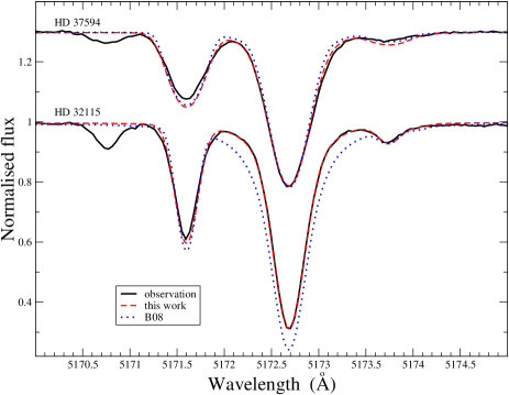
Figure 3: Comparison between the observed Mg i line profile of the line at $\lambda$ 5172 Å (black solid line) and synthetic profiles calculated with our final adopted parameters (red dashed line) and with the parameters adopted by B08 (blue dotted line). The upper comparison is for HD 37594, while the lower comparison is for HD 32115. The profiles shown for HD 37594 were rigidly shifted upwards of 0.3. Our synthetic profiles are calculated adopting the oscillator strength from Aldenius et al. (2007), damping constant from Barklem & O’Mara (2000) and a LTE Mg abundance of -4.50 dex for HD 32115 and -4.77 dex for HD 37594. B08 does not provide a Mg abundance for HD 37594, therefore we derived it from the Mg i line at $\lambda$ 5528 Å, adopting the parameters given in their paper.

Figure 3 shows an excellent agreement between the synthetic profiles calculated with our final adopted parameters and the observed spectrum. On the other hand, the synthetic profiles calculated with B08’s parameters display a disagreement with the observations, in particular for HD 32115. For HD 37594 the discrepancy is rather small: the effect of the higher $T_{\mathrm{eff}}$ is mostly compensated by the lower gravity.

The other two Mg i lines of the triplet ($\lambda\lambda$ 5167 and 5183 Å) will provide the same results we obtained with the $\lambda$ 5172 Å Mg i line, as tested by R09 with the Sun, Procyon and HD 49933.

For HD 32115, we used the stellar mass and bolometric magnitude by Fekel et al. (2006), in addition to our $T_{\mathrm{eff}}$, to derive $\log g$: $\log(g/g_{\odot})=\log(M/M_{\odot})+4\cdot\log(T_{\mathrm{eff}}/T_{eff,\odot})+0.4\cdot(M_{\mathrm{bol}}-4.75).$ We obtained a $\log g$ value of 4.24, in good agreement with our previous estimation and with the results by Fekel et al. (2006) and Allende Prieto & Lambert (1999).

3.2.3 Metallic lines

The metallic-line spectrum provides further constraints on the atmospheric parameters. If no deviation from LTE is expected, there should be no trend in individual line abundances as a function of excitation potential. Examining this for any element/ion therefore provides a check on the determined value of $T_{\mathrm{eff}}$. The balance between different ionisation stages of the same element similarly provides a check on $\log g$. The microturbulent velocity ($\upsilon_{\mathrm{mic}}$) is subsequently determined by minimising any trend between individual abundances and equivalent widths for a certain ion. Determining the fundamental parameters in this way must be done iteratively since, for example, a variation in $T_{\mathrm{eff}}$ leads to a change in the best $\log g$ and $\upsilon_{\mathrm{mic}}$. This methodology of fundamental parameter determination from the metallic line spectrum is adopted in almost all semi-automatic abundance analysis procedures (e.g. Bruntt et al. 2002; Santos et al. 2004; Gillon & Magain 2006).

The analysis of the metallic line spectrum requires the best possible knowledge of atomic line parameters, $\log{gf}$ values in particular. In this work we only use lines of Ca, Ti, Cr, and Fe for which experimental atomic parameters are available (except for Cr ii, as clarified later in the text). Atomic parameters were extracted from the VALD database and from other recent publications, see references in Table 2.

Data for neutral and ionised Ca lines were validated with non-LTE calculations by Mashonkina et al. (2007). For Ti i, Ti ii, Cr i and Fe i lines, accurate laboratory data (lifetimes and branching ratio) are available. For lines of ionised iron the oscillator strengths, selected from VALD, were produced from laboratory data, as explained in Ryabchikova et al. (1999). All corresponding references are given in Table 2. Laboratory data for optical Cr ii lines are scarce, therefore we took into account two different sets of calculated data, the one from semi-empirical orthogonal operator calculations by Raassen & Uylings (1998), and the one from the latest calculations by R. Kurucz. The lifetimes calculated by the two groups agree very well and are very close to recent laboratory lifetime measurements by Nilsson et al. (2006) and Gurell et al. (2010). A small difference between theoretical and experimental lifetimes, converted to a difference in oscillator strength, corresponds to a $\log{gf}$-value uncertainty no larger than $\pm$0.03 dex. However, the two sets of calculated oscillator strengths, for the lines used in our analysis, differ by 0.2 dex, as a result of different branching factors, as the lifetimes are practically identical. From two theoretical sets of oscillator strengths, Raassen & Uylings (1998)’s data provide us with a smaller standard deviation from the mean Cr ii abundance, while Kurucz’s data give a mean abundance closer to that derived from the Cr i lines. Clearly, an extensive laboratory analysis of Cr ii lines in the optical region is needed for the interpretation of the Cr abundance in atmospheres of cool and hot stars.

LTE line abundances were based on equivalent widths, analysed with a modified version (Tsymbal 1996) of the WIDTH9 code (Kurucz 1993). For blended lines and lines situated in the wings of the hydrogen lines we derived the line abundance performing synthetic spectrum calculations with the SYNTH3 code, tuning $\upsilon_{\mathrm{macro}}$ line by line (see Sect. 4.2.2). A line-by-line abundance list with the equivalent width measurements, adopted oscillator strengths, and their sources is given in Table 2 (see the online material for the complete version of the table). Table 2 also gives equivalent width measurements for the lines which we measured via spectral synthesis. In these cases, equivalent widths were tuned to match the abundance obtained with spectral synthesis. Our analysis shows that it is practically impossible to get a unique value of the microturbulent velocity for all considered species, therefore we derive a value that satisfies all the data and still provides a small scatter.

Table 2: Lines used for the parameter determination. Wavelengths and excitation potentials are taken from the VALD database. The adopted $\log{gf}$ values are taken from different sources which are listed in the last column. “S” in the equivalent with column denotes line abundances determined by fitting the observed line profile, with the equivalent width determined from the line abundance. The $\log{gf}$ values by Blackwell et al. (1980) and Baschek et al. (1970) were corrected by +0.2 and +0.16, respectively. For Cr ii the results obtained with two different sets of $\log{gf}$ values are given (see the Sect. 3.2.3). For each ion, the last line gives the average abundance and the standard deviation, with the number of lines in parenthesis. The entire table can be viewed in the electronic version of the Journal.

Element			HD 37594		HD 32115
Wavelength	$\chi_{\mathrm{excit}}$	$\log{gf}$	EQW	abundance	EQW	abundance	Ref $\log{gf}$
Å	eV		mÅ	dex	mÅ	dex
Ca i
4425.4370	1.8790	-0.358	S 100.0	-6.00	112.71	-5.70	SN
4435.6790	1.8860	-0.517	S 90.0	-6.00			SN
4526.9280	2.7090	-0.548			54.80	-5.78	SR
4578.5510	2.5210	-0.697	43.00	-5.99	54.75	-5.75	SR+Sm
4685.2680	2.9330	-0.879	21.46	-5.90	27.60	-5.70	S
5261.7040	2.5210	-0.579	S 46.0	-6.08			SR+Sm
5512.9800	2.9330	-0.464	39.77	-6.00	47.26	-5.83	SR+Sm
5581.9650	2.5230	-0.555	55.26	-5.97	64.10	-5.78	SR+Sm
5588.7490	2.5260	0.358	125.68	-5.84			SR+Sm
…	…	…	…	…	…	…	…

S - Smith (1988);
Sm - Smith (1981);
SN - Smith & O’Neil (1975);
SR - Smith & Raggett (1981);
…

Figures 4 and 5 show the correlations of Fe i and Fe ii abundance with equivalent width (left panels) and with excitation potential (right panels), respectively for HD 32115 and HD 37594. In each Figure, we used our final adopted fundamental parameters for the top panels and B08’s fundamental parameters for the bottom panels. B08 derived the effective temperature by imposing the excitation equilibrium for the Fe i lines only, the surface gravity by imposing the ionisation equilibrium for Fe i only, and the microturbulence velocity by removing the correlation between abundance and equivalent widths for Fe i lines only.

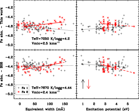
Figure 4: Individual abundances for Fe i (black crosses) and Fe ii (red asterisks) lines versus the equivalent width (left panels) and the excitation energy of the lower level (right panels) for HD 32115, with different model atmospheres. The top panels are for our adopted fundamental parameters, while the bottom panels are for B08’s fundamental parameters. The linear fit to the Fe i (black solid line) and Fe ii (red dashed line) data are also shown. The black cross and red asterisk at negative equivalent widths show respectively the mean Fe i and Fe ii abundance with their standard deviation. The black and red arrows show the direction of the non-LTE corrections for Fe i (upwards/higher abundance) and Fe ii (downwards/lower abundance), respectively.

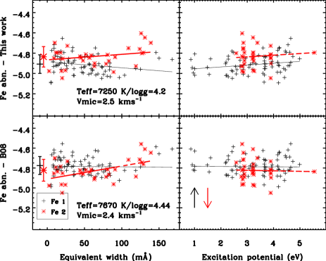
Figure 5: Same as in Fig. 4, but for HD 37594.

With our model parameters for HD 32115, we get a small positive correlation for Fe i abundance, and a small anti-correlation for Fe ii abundance, with the excitation potential. Our adopted $T_{\mathrm{eff}}$ thus accommodates both Fe i and Fe ii. With our model parameters for HD 37594, we get a small positive correlation for both Fe i and Fe ii abundance with the excitation potential. These correlations would change slightly by adopting a different set of Fe lines, even by adding or removing a few lines, making the parameter determination based on these correlations rather sensitive to systematic effects introduced by the line selection. One example is the high excitation energy Fe ii line, shown in Figs. 4 and 5, which has a much larger influence on the Fe ii excitation equilibrium, compared to the other Fe ii lines.

The model parameters obtained by B08 lead to almost perfect equilibria for Fe i, as requested by B08 analysis method; in the case of HD 32115, B08’s $T_{\mathrm{eff}}$ is anyway so high that even the excitation equilibrium for Fe i is not reached, although it is imposed by their analysis method.

The equilibria for Fe i are reached better with B08’s parameters, compared to ours, as it is the only $T_{\mathrm{eff}}$ and $\upsilon_{\mathrm{mic}}$ indicator they used, but it leads to a set of parameters which does not fit all the other parameter indicators, first of all Fe ii.

The average abundances, shown in Figs. 4 and 5, show that we obtain the ionisation equilibrium for Fe, within the error bars. We notice also that our average Fe ii abundance is systematically higher by a few 0.01 dex, compared to Fe i, in agreement with non-LTE calculations by Mashonkina (2011) (the direction of the Fe non-LTE corrections is shown in Figs. 4 and 5). Adopting B08’s parameters, we obtain a systematically lower Fe ii abundance, compared to Fe i, and the non-LTE corrections by Mashonkina (2011) would then worsen the ionisation equilibrium, indicating that B08’s sets of parameters is inappropriate for these stars.

Figure 6 shows the line abundance versus the equivalent widths for Ca, Ti, and Cr, in HD 32115 and HD 37594, adopting our final fundamental parameters. As for Fe, these elements display a variety of small correlations and on average our fundamental parameters are the ones which suit at best all considered ions. The ionisation equilibrium is reached within the error bars for all elements considered here, except Cr, for which the equilibrium is obtained adopting Kurucz’s oscillator strengths, as shown in Table 2. Also with laboratory data for Cr lines, we expect an improvement in the Cr ionisation equilibrium.

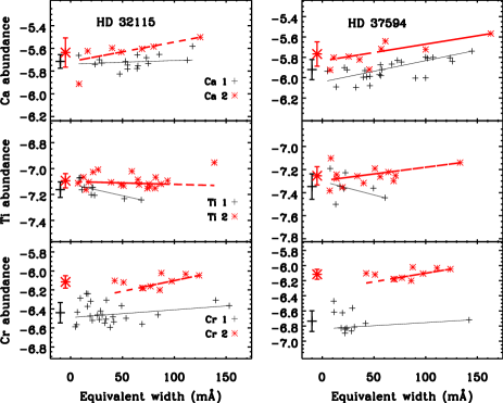
Figure 6: Individual abundances for Ca (top panels), Ti (middle panels), and Cr (bottom panels) lines versus the equivalent width measured for HD 32115 (left panels) and HD 37594 (right panels). In each panel, the black crosses indicate the lines of neutral elements, while the red asterisks indicate the lines of singly ionised elements. All abundances are derived assuming our adopted fundamental parameters. The linear fits to the data are also shown. The black cross and red asterisk at negative equivalent widths show the average abundance respectively for the neutral and singly ionised elements, with their standard deviation. The poor Cr ionisation equilibrium is most likely due to the poor quality line data.

4 Discussion

For HD 32115 our final adopted set of parameters is: $T_{\mathrm{eff}}$ = 7250$\pm$100 K, $\log g$ = 4.2$\pm$0.1 and $\upsilon_{\mathrm{mic}}$ = 2.5$\pm$0.2 $\mathrm{km\,s}^{-1}$. For HD 37594 we derived $T_{\mathrm{eff}}$ = 7150$\pm$100 K, $\log g$ = 4.2$\pm$0.1 and $\upsilon_{\mathrm{mic}}$ = 2.6$\pm$0.2 $\mathrm{km\,s}^{-1}$. The measured projected rotational velocity (${\upsilon}\sin i$) is 8.3 and 17.0 $\mathrm{km\,s}^{-1}$, respectively for HD 32115 and HD 37594. The observed line profiles required also a substantial macroturbulence velocity ($\upsilon_{\mathrm{macro}}$), generally between 8 and 10 $\mathrm{km\,s}^{-1}$ for both stars (see Sect. 4.2.2 for more details). These high values of $\upsilon_{\mathrm{macro}}$ are in line with an extrapolation of the $\upsilon_{\mathrm{macro}}$$T_{\mathrm{eff}}$ correlations given by Valenti & Fisher (2005) and Bruntt et al. (2010).

Our fundamental parameters are not perfect, by definition, but they provide, within the error bars, the best description of all available observables: photometric colors, hydrogen and metallic line profiles.

4.1 Model fluxes and observed photometry

Other methods which should always be used to check the fundamental parameters obtained by spectroscopic means are: i) comparison of synthetic and observed optical colors; ii) comparison between photometry, calibrated in flux, and synthetic spectral energy distribution (SED). We performed these comparisons for HD 32115 and HD 37594, aiming also to estimate the precision which can be reached with these two methods.

4.1.1 Synthetic colors

Table 3 summarises the comparison between observed and theoretical color-indexes for different photometric systems for the two stars, adopting the fundamental parameters obtained in this work and by B08. We highlight the better agreeing theoretical index in each case. Overall out values provide better matches. All colors were calculated using modified computer codes by Kurucz (1993), which take into account transmission curves of individual photometric filters, mirror reflectivity and a photomultiplier response function. In contrast to Kurucz’s procedures (Relyea & Kurucz 1978) which are based on the low resolution theoretical fluxes, our synthetic colors are computed from energy distributions sampled with a fine wavelength step, so integration errors are expected to be small.

Table 3: Observed and calculated photometric parameters of HD 32115 and HD 37594. The values in brackets give the error bars of observations. The better agreeing theoretical index in each case is highlighted.

	HD 32115			HD 37594
Color	Observed	t7250g4.2	t7670g4.44	Observed	t7150g4.20	t7380g4.08
index	photometry	this work	B08	photometry	this work	B08
Johnson
$U$-$B$	0.040	0.0316	0.0368	0.010	0.0002	0.0290
$B$-$V$	0.285	0.2943	0.2432	0.275	0.2964	0.2530
Strömgren
$b$-$y$	0.176	0.1904	0.1463	0.189	0.1982	0.1668
	(0.003)			(0.001)
$m_{\rm 1}$	0.181	0.1787	0.2023	0.160	0.1621	0.1674
	(0.005)			(0.005)
$c_{\rm 1}$	0.689	0.7044	0.7399	0.669	0.6806	0.7832
	(0.003)			(0.007)
$H\beta$	2.753	2.8077	2.8502	2.738	2.7924	2.8180
	(0.004)			(0.005)
Geneva
$U$-$B$	1.389	1.3972	1.4041	1.354	1.3646	1.4298
$V$-$B$	0.611	0.6160	0.6732	0.606	0.6161	0.6658
$B_{\rm 1}$-$B$	0.963	0.9823	0.9769	0.950	0.9728	0.9639
$B_{\rm 2}$-$B$	1.416	1.4190	1.4255	1.423	1.4273	1.4371
$V_{\rm 1}$-$B$	1.328	1.3371	1.3901	1.324	1.3376	1.3844
$G$-$B$	1.734	1.7478	1.8217	1.720	1.7465	1.8077

To fully understand Table 3, it is first necessary to establish more in general how well synthetic colors can reproduce the observations. This can be done by comparing synthetic and observed colors for well known stars. To check the quality of synthetic and observed colors over a large temperature range, we examine three “standard” stars with different temperatures: Procyon ($T_{\mathrm{eff}}$=6530 K; Fuhrmann et al. 1997), Vega ($T_{\mathrm{eff}}$=9550 K; Castelli & Kurucz 1994), and 21 Peg ($T_{\mathrm{eff}}$=10400 K; Fossati et al. 2009).

Figure 7 shows a comparison between synthetic and observed colors for the three reference stars, plus HD 32115 and HD 37594. With a few exceptions, there is general good agreement between synthetic and observed colors throughout the temperature region explored here. For 21 Peg, there is difference of 0.04 mag between synthetic and observed $U-B$ Johnson color, $V_{\rm 1}$-$B$ and $G$-$B$ Geneva colors. This difference is most likely due to incorrect photometry in one (or more) photometric band, as there is a perfect agreement between synthetic spectral energy distribution and spectrophotometry in the whole wavelength region between the near-UV and the near infrared (see Fig. 4 by Fossati et al. 2009). On the other hand we do not have an explanation for the difference of 0.03 mag obtained between synthetic and observed $b-y$ Strömgren color for Procyon, although an error in the photometry is always possible, even for such a bright star. Besides these two exceptions, there is general agreement between synthetic and observed colors at a 0.01–0.02 mag level, which represents then the typical precision that one can expect for the comparison between observed and synthetic colors.

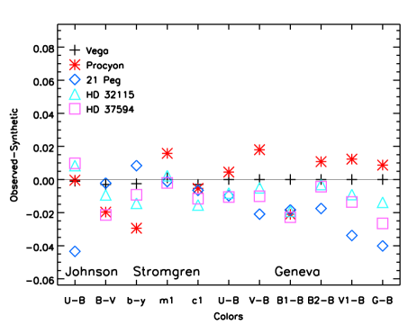
Figure 7: Comparison between observed and synthetic colors for a set of reference stars, plus HD 32115 (bright blue triangles) and HD 37594 (violet squares). The reference stars are: Vega (black crosses), Procyon (red asterisks), and 21 Peg (blue diamonds). Photometric colors are labelled on the X-axis. For all stars we assumed zero interstellar reddening.

Figure 7 shows that for HD 32115 and HD 37594 the difference between synthetic and observed colors is within the typical precision obtained for the “reference” stars, confirming the quality of our fundamental parameters. Figure 8 shows that a comparison between observed and synthetic colors calculated with B08’s stellar parameters clearly demonstrate the inadequacy of the B08 fundamental parameters.

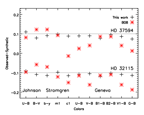
Figure 8: Comparison between observed and synthetic colors for HD 32115 (shifted downwards of 0.1) and HD 37594 (shifted upwards of 0.1). The colors calculated with our final set of parameters and B08’s parameters are shown by black crosses and red asterisks, respectively. Photometric colors are labelled on the xaxis. For both stars we assumed zero interstellar reddening.

4.1.2 Spectral energy distribution

For a complete self-consistent analysis of any star, one should reproduce the observed spectral energy distribution with the adopted parameters for a model atmosphere. For HD 32115 and HD 37594 no spectrophotometry is available, therefore we converted the available Johnson (Johnson et al. 1966), Geneva (Rufener 1988) and 2MASS (Zacharias et al. 2005) photometry into physical units and compared them with the model fluxes calculated with the final set of parameters derived for the two stars. In the case of the Geneva colors, we assumed that Geneva $V_{\rm G}$ index is close to Johnson $V_{\rm J}$, making then possible to recover the Geneva $B$ index and thus $U$, $B_{\rm 1}$, $B_{\rm 2}$, $V_{\rm 1}$, and $G$, and to transform them to absolute fluxes using the calibrations given by Rufener & Nicolet (1988). For the 2MASS ($JHK$) photometry we employed calibrations by van der Bliek et al. (1996), while for the Johnson photometry we employed calibrations by Bessell et al. (1998).

Figure 9 shows the comparison between the observed photometry (in physical units) and the model fluxes calculated with the adopted atmospheric parameters for HD 32115 and HD 37594. There is a good agreement between observed and synthetic fluxes in the visible and infrared regions, providing a further confirmation of our adopted stellar parameters for the two stars.

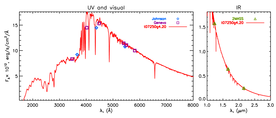
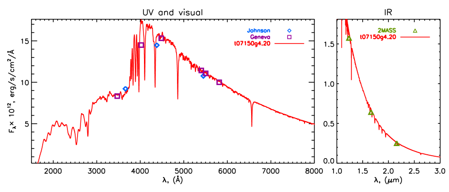
Figure 9: Comparison between LLmodels theoretical fluxes (full red lines) calculated with the fundamental parameters derived for HD 32115 (upper panel) and HD 37594 (lower panel), with Johnson, Geneva (respectively open diamonds and squares in the left panels) and 2MASS (open triangles in the right panels) photometry converted to physical units.

Precise HIPPARCOS parallaxes are available for both stars (van Leeuwen 2007). This allowed us also to estimate their radii: 1.52$\pm$0.04 $R_{\odot}$ for HD 32115 and 1.36$\pm$0.02 $R_{\odot}$ for HD 37594. The radius we derived for HD 32115 is in very good agreement with what previously obtained by Fekel et al. (2006) and Allende Prieto & Lambert (1999), who measured the stellar radius by means of stellar evolution calculations. This comparison increases the confidence on our results.

4.2 Classic vs. semi-automatic procedures

The most evident difference between the analysis performed by B08 and our analysis (including HD 49933 by R09) is that B08 did not add any $\upsilon_{\mathrm{macro}}$ to the line broadening. Since B08 used line profile fitting, instead of equivalent widths, the lack of the additional broadening renders their whole analysis questionable. Bikmaev et al. (2002) also did not use any $\upsilon_{\mathrm{macro}}$ in their analysis, but their spectra were of mid-low resolution and therefore ${\upsilon}\sin i$ was enough to fit the lines and their abundance analysis was based mainly on equivalent widths, independent of $\upsilon_{\mathrm{macro}}$. At the resolution of CORALIE and TS ($R$=50 000 and 60 000, respectively), line profiles clearly require an additional $\upsilon_{\mathrm{macro}}$ broadening.

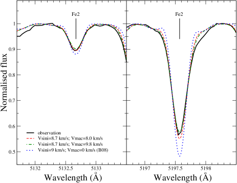
Figure 10: Observed HD 32115 line profiles (black solid line) of two Fe ii lines at $\lambda$5132 Å (left panel) and $\lambda$5197 Å (right panel) in comparison with three synthetic spectra calculated with three different sets of broadening parameters: ${\upsilon}\sin i$=8.7 $\mathrm{km\,s}^{-1}$ and $\upsilon_{\mathrm{macro}}$=8.0 $\mathrm{km\,s}^{-1}$ (red dashed line); vsini=8.7 $\mathrm{km\,s}^{-1}$ and $\upsilon_{\mathrm{macro}}$=9.8 $\mathrm{km\,s}^{-1}$ (green dotted-dashed line); ${\upsilon}\sin i$=9.0 $\mathrm{km\,s}^{-1}$and $\upsilon_{\mathrm{macro}}$=0 $\mathrm{km\,s}^{-1}$(blue dotted line). The first set of parameters fits the weak lines best, the second the strong lines, while the third is the one adopted by B08. For all three synthetic spectra we used our final set of fundamental parameters and abundances.

Figure 10 compares the observed HD 32115 line profiles of two Fe ii lines, one weak and one strong, with three synthetic spectra calculated with our adopted parameters and three different sets of broadening parameters. The three broadening parameter sets are suited to weak lines, strong lines, and one as given by B08, respectively.

The difference in $\upsilon_{\mathrm{macro}}$ between weak and strong lines is found systematically for several lines of the same ion, and for different ions, excluding the possibility that this is due to an error in $\upsilon_{\mathrm{mic}}$, ${\upsilon}\sin i$, or in the damping constants (homogeneous calculations by Barklem et al. 2000; Barklem & Aspelund-Johansson 2005). This systematic difference in $\upsilon_{\mathrm{macro}}$ between weak and strong lines was found also by Fuhrmann et al. (1997) in their analysis of Procyon.

The profiles calculated using the broadening by B08 show too deep cores and too narrow wings. This implies that B08 systematically obtained erroneously high $T_{\mathrm{eff}}$ for the three stars (HD 49933, HD 32115, and HD 37594) to compensate for the deeper line cores, as a result of neglecting $\upsilon_{\mathrm{macro}}$ and fitting line cores to derive the abundances. This is confirmed by the fact that Bruntt (2009) reanalysed HD 49933, adopting a $\upsilon_{\mathrm{macro}}$ of 2 $\mathrm{km\,s}^{-1}$, and obtained a much lower temperature than given in B08. It is still not clear to us where this particular value of $\upsilon_{\mathrm{macro}}$ came from, as R09 measured a $\upsilon_{\mathrm{macro}}$ of 5.2$\pm$0.5 $\mathrm{km\,s}^{-1}$, in agreement with the calibration by Valenti & Fisher (2005). Figure 10 demonstrates that even adopting all the parameters and abundances given by B08, it is impossible to simultaneously fit the line profiles of weak and strong lines, as the wings will always be too narrow and the higher $T_{\mathrm{eff}}$ cannot compensate for it.

One of our main goals was to find and analyse possible sources of discrepancies between the results obtained with a classical method of analysis (e.g. this work and R09) and with a semi-automatic procedure (e.g. Bruntt et al. 2008; Bruntt 2009). We have identified two possible sources of discrepancy. The first arises from semi-automatic procedures often taking into account only Fe i lines to derive $T_{\mathrm{eff}}$ and $\upsilon_{\mathrm{mic}}$, while the second arises from the nature of the line profiles for these stars.

4.2.1 Is Fe i alone good enough for a precise parameter determination?

The upper-left panel of Fig. 4 shows the Fe i and Fe ii line abundance as a function of equivalent width, used for the determination of the microturbulence velocity. It is clear that a perfect equilibrium between the line abundance and equivalent width is not reached, and not simultaneously reachable, as the two ions show opposite correlations: $-5.524\pm 2.407$ and $6.402\pm 3.676$, in units of 10^-4, respectively for Fe i and Fe ii. Something similar is found for the ions of other species, as both Ca and Cr show a positive correlation, while Ti shows a negative correlation (see Fig. 6).

The $\upsilon_{\mathrm{mic}}$ value we adopted considers the effects on all the ions we took into account, whereas the $\upsilon_{\mathrm{mic}}$ value derived from the Fe i lines alone, worsens the situation for Fe ii and Ti, resulting in a systematic underestimation of $\upsilon_{\mathrm{mic}}$. Bruntt et al. (2010) presented a calibration of $\upsilon_{\mathrm{mic}}$ as a function of $T_{\mathrm{eff}}$ for late-type stars, based on the analysis of Fe i lines alone, therefore this calibration could also underestimate $\upsilon_{\mathrm{mic}}$.

Using Fe i lines alone for the determination of $\upsilon_{\mathrm{mic}}$ means that the average Fe ii abundance depends strongly on which lines have been selected. If the selected Fe ii lines are predominantly weak, the Fe ii abundance will be artificially low. This introduces a bias in the determination of the surface gravity, as most semi-automatic procedures employ the Fe ionisation equilibrium alone to measure $\log g$. The use of predominant medium-to-weak Fe ii lines, with the adoption of Fe i lines alone to determine $\upsilon_{\mathrm{mic}}$ consequently leads to a sistematically erroneously low Fe ii abundance, which then causes an erroneously high $\log g$ to be inferred. This of course, then affects the value of $T_{\mathrm{eff}}$.

Another problem connected to the use of Fe i lines as the sole temperature indicator is shown in the top-right panel of Fig. 4. The effective temperature which best fits all available observables does not completely remove the correlation between abundance and excitation potential. For HD 32115, by adopting only Fe i as a $T_{\mathrm{eff}}$ and $\upsilon_{\mathrm{mic}}$ indicator, and only Fe for the ionisation equilibrium, we derived $T_{\mathrm{eff}}$=7400 K, $\log g$=4.2, and $\upsilon_{\mathrm{mic}}$=2.4 $\mathrm{km\,s}^{-1}$. Similarly, for HD 37594 we obtained $T_{\mathrm{eff}}$=7300 K, $\log g$=4.1, and $\upsilon_{\mathrm{mic}}$=2.5 $\mathrm{km\,s}^{-1}$. These temperatures are too high and cannot fit the hydrogen lines or the photometry, with photometric colors revealing the discrepancies.

The adoption of Fe i alone as $T_{\mathrm{eff}}$ and $\upsilon_{\mathrm{mic}}$ indicator might also lead to the presence of systematic errors in the fundamental parameters arising from non-LTE effects. This is particularly true for cool stars, where non-LTE effects are larger for Fe i than Fe ii, with obvious consequences for i.e. $\log g$. Non-LTE effects are generally stronger for stronger lines, implying that systematic errors might be introduced in the determination of $\upsilon_{\mathrm{mic}}$, consequently affecting $T_{\mathrm{eff}}$ as well.

All problems described here can be solved by including other ions in the process of parameter determination. Although fewer lines of ions other than Fe i are usually available, their inclusion in the parameter determination procedure would significantly alleviate the systematic errors introduced by the use of only Fe i lines.

Asplund et al. (2005) shows differences between 3D and 1D LTE abundances for several ions as a function of the excitation potential for the Sun. For Fe i, the 1D models, compared to the 3D models, lead to a deviation as large as 0.2 dex for the low excitation lines, which decreases with increasing excitation potential. Clearly, the use of 1D models introduces a strong bias towards high temperatures. This effect is present, with slightly different strengths, for many other ions. It would be extremely valuable to study this effect for stars hotter than the Sun, where the registered high $\upsilon_{\mathrm{macro}}$ values suggest that hydrodynamical effects might be even stronger than in the Sun.

4.2.2 The effect of macroturbulence

Valenti & Fisher (2005) and Bruntt et al. (2010) showed that for late-type stars the macroturbulence velocity ($\upsilon_{\mathrm{macro}}$) increases with increasing $T_{\mathrm{eff}}$. For HD 32115 and HD 37594, $\upsilon_{\mathrm{macro}}$ reaches rather high values, close to 10 $\mathrm{km\,s}^{-1}$. During the analysis of the spectra of the two stars, we noticed a systematic difference between the line profiles of strong and weak lines, as strong lines require a systematically higher $\upsilon_{\mathrm{macro}}$ compared to weak lines, by $\sim$2 $\mathrm{km\,s}^{-1}$, as shown in Fig. 10. We believe that this difference is due to unmodelled depth-dependent velocities in the atmosphere which become evident for stars with relatively high $\upsilon_{\mathrm{macro}}$ and low ${\upsilon}\sin i$.

This is not a concern if the abundances are derived from equivalent widths, as they are independent of macroturbulence velocity. On the other hand, if the abundances are obtained from line profile fitting, where the abundance is the only free parameter, a systematic abundance difference is introduced between strong and weak lines, affecting the determination of the fundamental parameters.

Semi-automatic abundance analysis procedures first set the broadening parameters to the entire available spectrum and then measure the line abundance from line profile fitting. If strong and weak lines require different broadening, opposing biases are introduced in the abundances derived from weak and strong lines. We estimated that the abundances obtained by fitting the profile of strong lines, adopting a $\upsilon_{\mathrm{macro}}$ typical for weak lines, are systematically lower by 0.10–0.15 dex, compared to the abundances obtained with a $\upsilon_{\mathrm{macro}}$ appropriate to strong lines. Consequently the abundances obtained from weak and strong lines will be systematically over- and under-estimated, respectively.

The systematic effect described above might be temperature and ${\upsilon}\sin i$ dependent as the difference in $\upsilon_{\mathrm{macro}}$ between weak and strong lines could increase with increasing $T_{\mathrm{eff}}$, and be more evident with decreasing ${\upsilon}\sin i$. In fact, the worst situation may be for slowly rotating “cool” early-type stars, such as HD 32115.

The problem described here can be solved using equivalent widths, instead of line profile fitting, as the equivalent widths are broadening independent. Alternatively $\upsilon_{\mathrm{macro}}$ could be treated as a further free parameter in the line profile fitting, although thorough tests on the uniqueness of the derived line abundance and $\upsilon_{\mathrm{macro}}$ should be performed. The adoption of 3D atmosphere models would also partly eliminate this problem, but this is not a viable solution for an abundance analysis of a large sample of stars.

5 Conclusion

On the basis of high resolution, high signal-to-noise ratio spectra, taken at the McDonald observatory, we carried out a precise parameter determination of two late A-type stars, HD 32115 and HD 37594, which Bruntt et al. (2008) adopted as reference stars for their abundance analysis of $\gamma$ Dor stars. Bruntt et al. (2008) analysed these stars with a semi-automatic procedure and their results strongly disagreed with those previously obtained by Bikmaev et al. (2002), by means of a “classical” analysis. This discrepancy, together with that previously highlighted by Ryabchikova et al. (2009) for HD 49933, prompted us to reanalyse HD 32115 and HD 37594 to look for the origin of the discrepancies.

We derived the fundamental parameters making use of all the available observables: multicolor photometry, pressure-sensitive magnesium lines, metallic lines and profiles of hydrogen Balmer lines. For HD 32115 our final adopted set of parameters is: $T_{\mathrm{eff}}$ = 7250$\pm$100 K, $\log g$ = 4.2$\pm$0.1 and $\upsilon_{\mathrm{mic}}$ = 2.5$\pm$0.2 $\mathrm{km\,s}^{-1}$. For HD 37594 we adopted: $T_{\mathrm{eff}}$ = 7150$\pm$100 K, $\log g$ = 4.2$\pm$0.1 and $\upsilon_{\mathrm{mic}}$ = 2.6$\pm$0.2 $\mathrm{km\,s}^{-1}$. We confirmed our final set of parameters by comparing flux calibrated photometry with synthetic spectral energy distributions, and by comparing observed and synthetic photometric colors. Our prefered fundamental parameters fit, within the error bars, all available observables. They are also in agreement with the results by Bikmaev et al. (2002), but disagree with the results by Bruntt et al. (2008). For HD 32115, our set of parameters agrees with that previously obtained by Fekel et al. (2006) and Allende Prieto & Lambert (1999). In addition, the radius of HD 32115, we derived from the analysis of the spectral energy distribution, is in perfect agreement with that derived by Fekel et al. (2006) and Allende Prieto & Lambert (1999) by means of stellar evolution calculations.

We compared our McDonald spectra with those used by Bruntt et al. (2008) and Bikmaev et al. (2002), concluding that the differences between the three set of spectra is well within the given S/N. The quality of the data is not the origin of the discrepancies.

To fit the line profiles of the two stars, we had to adopt rather large $\upsilon_{\mathrm{macro}}$ values, between 8 and 10 $\mathrm{km\,s}^{-1}$. Although the spectra analysed by Bruntt et al. (2008) had enough resolution to require the need of $\upsilon_{\mathrm{macro}}$ to fit line profiles, they adopted only rotational broadening (${\upsilon}\sin i$) in their spectral synthesis. As a consequence, by deriving the line abundance by fitting synthetic line profiles to the observed ones, discarding any $\upsilon_{\mathrm{macro}}$ broadening, they introduced a bias in their analysis, which we believe led them to an erroneous set of fundamental parameters.

We have demonstrated that the determination of $T_{\mathrm{eff}}$ and $\log g$ using only the Fe i excitation equilibrium and the Fe ionisation equilibrium leads to a systematic higher $T_{\mathrm{eff}}$ compared to that suggested by all other indicators. We also believe that this effect might be temperature dependent.

Several automatic and semi-automatic procedures use the Fe i excitation equilibrium and the Fe ionisation equilibrium as only/primary indicators for stellar parameter determination. In this work we show that these procedures do not always provide the correct set of fundamental parameters and their results need to be cautiously taken when performing further analysis, such as modelling of the asteroseismic frequencies or the characterisation of transiting exoplanets.

Table 4: Lines used for the parameter determination. Wavelengths and excitation potentials are taken from the VALD database. The adopted $\log{gf}$ values are taken from different sources which are listed in the last column. “S” in the equivalent with column denotes line abundances determined by fitting the observed line profile, with the equivalent width determined from the line abundance. The $\log{gf}$ values by Blackwell et al. (1980) and Baschek et al. (1970) were corrected by +0.2 and +0.16, respectively. For Cr ii the results obtained with two different sets of $\log{gf}$ values are given (see the Sect. 3.2.3). For each ion, the last line gives the average abundance and the standard deviation, with the number of lines in parenthesis.

Element			HD 37594		HD 32115
Wavelength	$\chi_{\mathrm{excit}}$	$\log{gf}$	EQW	abundance	EQW	abundance	Ref $\log{gf}$
Å	eV		mÅ	dex	mÅ	dex
Ca i
4425.4370	1.8790	-0.358	S 100.0	-6.00	112.71	-5.70	SN
4435.6790	1.8860	-0.517	S 90.0	-6.00			SN
4526.9280	2.7090	-0.548			54.80	-5.78	SR
4578.5510	2.5210	-0.697	43.00	-5.99	54.75	-5.75	SR+Sm
4685.2680	2.9330	-0.879	21.46	-5.90	27.60	-5.70	S
5261.7040	2.5210	-0.579	S 46.0	-6.08			SR+Sm
5512.9800	2.9330	-0.464	39.77	-6.00	47.26	-5.83	SR+Sm
5581.9650	2.5230	-0.555	55.26	-5.97	64.10	-5.78	SR+Sm
5588.7490	2.5260	0.358	125.68	-5.84			SR+Sm
5590.1140	2.5210	-0.571	57.83	-5.92	64.85	-5.75	SR+Sm
5601.2770	2.5260	-0.523	56.75	-5.98	73.14	-5.68	SR+Sm
5857.4510	2.9330	0.240	101.96	-5.81			S+Sm
5867.5620	2.9330	-1.570	4.87	-5.94	7.73	-5.66	S
6122.2170	1.8860	-0.316	123.55	-5.80			SN
6161.2970	2.5230	-1.266	13.42	-6.09	23.49	-5.74	SR+Sm
6162.1730	1.8990	-0.090	144.67	-5.74			SN
6166.4390	2.5210	-1.142	24.02	-5.92	30.20	-5.73	SR+Sm
6169.0420	2.5230	-0.797	32.57	-6.10	52.80	-5.71	SR+Sm
6169.5630	2.5260	-0.478	72.66	-5.83	74.77	-5.73	SR+Sm
6471.6620	2.5260	-0.686	45.97	-5.99	64.32	-5.66	SR+Sm
6493.7810	2.5210	-0.109	99.99	-5.80			SR+Sm
6499.6500	2.5230	-0.818	41.29	-5.93			SR+Sm
6717.6810	2.7090	-0.524	56.24	-5.87			SR
7148.1500	2.7090	0.137	107.26	-5.80	117.58	-5.58	SR
7202.2000	2.7090	-0.262	76.54	-5.85			SR
7326.1450	2.9330	-0.208	67.13	-5.87	85.61	-5.65	S
Average			-5.92$\pm$0.10 (25)		-5.71$\pm$0.06 (16)
Ca ii
5001.4790	7.5050	-0.507	S 36.00	-5.82	48.88	-5.63	TB
5019.9710	7.5150	-0.247	S 45.50	-5.92			TB
5021.1380	7.5150	-1.207	S 7.60	-5.92	8.00	-5.91	TB
5285.2660	7.5050	-1.147	S 11.10	-5.80	S 16.40	-5.62	TB
5339.1880	8.4380	-0.079	S 25.50	-5.79	S 40.00	-5.60	TB
6456.8750	8.4380	0.412	S 61.00	-5.64	80.00	-5.58	TB
8201.7220	7.5050	0.368	S 100.00	-5.72	125.03	-5.50	TB
8248.7960	7.5150	0.556	S 163.00	-5.57			TB
8254.7210	7.5150	-0.398	S 57.00	-5.72	68.79	-5.60	TB
Average			-5.77$\pm$0.12 (9)		-5.64$\pm$0.13 (7)
Ti i
4453.6990	1.8730	-0.010			9.30	-7.07	MFW
4548.7630	0.8260	-0.354	17.07	-7.34	20.80	-7.14	MFW
4617.2690	1.7490	0.389	13.00	-7.50	19.90	-7.20	MFW
4758.1180	2.2490	0.425			10.80	-7.16	MFW
4759.2700	2.2560	0.514			13.38	-7.14	MFW
4981.7310	0.8480	0.504	60.55	-7.44	68.20	-7.24	MFW
4999.5030	0.8260	0.250	49.47	-7.36	51.70	-7.23	MFW
5192.9690	0.0210	-1.006	22.40	-7.23	21.30	-7.15	MFW
5210.3850	0.0480	-0.884	20.84	-7.36	23.10	-7.21	MFW
6261.0980	1.4300	-0.479	7.67	-7.19	8.20	-7.07	MFW
Average			-7.35$\pm$0.11 (7)		-7.16$\pm$0.06 (10)
Ti ii
4394.0510	1.2210	-1.770			93.50	-7.09	BHN
4395.8389	1.2430	-1.970			74.00	-7.15	BHN
4411.9250	1.2240	-2.520	33.86	-7.26	39.00	-7.11	PTP
4417.7136	1.1650	-1.190	133.34	-7.14	138.58	-6.95	PTP
4418.3300	1.2370	-1.990	70.91	-7.25	75.50	-7.12	BHN
4421.9380	2.0610	-1.660	50.88	-7.19	59.00	-7.02	PTP
4444.5545	1.1160	-2.210	63.98	-7.22	66.00	-7.12	BHN
4470.8532	1.1650	-2.020			76.16	-7.14	PTP
4568.3140	1.2240	-2.940			21.63	-7.03	PTP
4609.2640	1.1800	-3.430	8.31	-7.10	7.07	-7.11	BHN
4636.3200	1.1650	-3.230	7.18	-7.38	12.35	-7.07	BHN
4657.2004	1.2430	-2.320			51.03	-7.13	BHN
4708.6621	1.2370	-2.370	40.00	-7.32	48.70	-7.12	BHN
4779.9850	2.0480	-1.260			81.50	-7.15	RHL
5005.1570	1.5660	-2.730	13.78	-7.28	17.44	-7.10	BHN
5185.9018	1.8930	-1.490	S 69.0	-7.30	82.00	-7.07	PTP
5252.0190	2.5900	-1.960	13.79	-7.24	14.86	-7.16	PTP
5336.7710	1.5820	-1.630			87.09	-7.12	BHN
5381.0150	1.5660	-1.970	56.00	-7.26	64.86	-7.09	BHN
7214.7160	2.5900	-1.740	19.60	-7.35	26.44	-7.01	MFW
Average			-7.25$\pm$0.08 (13)		-7.09$\pm$0.05 (20)
Cr i
4274.7970	0.0000	-0.231	S 142.0	-6.72	S 153.0	-6.37	MFW
4545.9530	0.9410	-1.370	22.29	-6.84	S 34.0	-6.51	SLS
4492.3050	3.3750	-0.392			9.32	-6.29	MFW
4616.1240	0.9830	-1.190	28.18	-6.87	41.63	-6.53	SLS
4646.1620	1.0300	-0.740			68.94	-6.56	SLS
4651.2840	0.9830	-1.460	18.32	-6.83	27.65	-6.51	SLS
4652.1570	1.0040	-1.040	41.90	-6.76	53.42	-6.50	SLS
4689.3570	3.1250	-0.400	11.00	-6.47	15.33	-6.24	SLS
4708.0130	3.1680	0.070	19.50	-6.62	20.79	-6.52	SLS
4718.4200	3.1950	0.240	29.00	-6.57	30.42	-6.46	SLS
4752.0870	4.1860	0.440			16.68	-6.24	MFW
4756.1120	3.1040	0.090			34.43	-6.31	MFW
4789.3350	2.5440	-0.330			28.78	-6.42	SLS
4922.2650	3.1040	0.380			49.08	-6.37	SLS
4936.3360	3.1130	-0.250	11.50	-6.61	16.30	-6.37	SLS
5206.0370	0.9410	0.020			140.00	-6.31	SLS
5247.5650	0.9610	-1.590			26.00	-6.46	SLS
5296.6910	0.9830	-1.360	23.50	-6.82	32.78	-6.55	SLS
5297.3770	2.9000	0.167	21.91	-6.89	40.75	-6.48	MFW
5348.3150	1.0040	-1.210	31.00	-6.82	38.04	-6.59	SLS
5409.7840	1.0300	-0.670			84.09	-6.46	SLS
5783.0630	3.3230	-0.500			4.51	-6.59	MFW
5787.9180	3.3220	-0.083			19.30	-6.32	MFW
6925.2720	3.4490	-0.330			5.82	-6.56	MFW
6978.3970	3.4640	0.142			18.87	-6.47	MFW
6979.7950	3.4640	-0.410			6.42	-6.43	MFW
Average			-6.74$\pm$0.14 (12)		-6.44$\pm$0.11 (26)
Cr ii
4145.7810	5.3190	-1.106			S 42.5	-6.10	RU
4252.6320	3.8580	-2.054	S 33.0	-6.44	S 51.0	-6.12	RU
4275.5670	3.8580	-1.736	S 54.0	-6.43	S 69.0	-6.18	RU
4554.9880	4.0710	-1.491	S 56.0	-6.50	S 77.0	-6.16	RU
4588.1990	4.0710	-0.845	S 107.0	-6.39	S 124.0	-6.05	RU
4592.0490	4.0740	-1.473	S 66.0	-6.37	S 87.5	-6.02	RU
4616.6290	4.0720	-1.576	S 56.0	-6.45	S 70.0	-6.18	RU
4618.8030	4.0740	-1.084	S 88.0	-6.45	S 111.0	-6.03	RU
4634.0700	4.0720	-1.236	S 81.0	-6.40	S 97.5	-6.11	RU
5237.3290	4.0730	-1.350	S 71.0	-6.45	S 86.0	-6.20	RU
Average			-6.43$\pm$0.04 (9)		-6.12$\pm$0.07 (10)
4145.7810	5.3190	-1.23			S 42.5	-5.98	K10
4252.6320	3.8580	-1.99	S 33.0	-6.50	S 51.0	-6.18	K10
4275.5670	3.8580	-1.67	S 54.0	-6.50	S 69.0	-6.25	K10
4554.9880	4.0710	-1.28	S 56.0	-6.71	S 77.0	-6.37	K10
4588.1990	4.0710	-0.63	S 107.0	-6.61	S 124.0	-6.27	K10
4592.0490	4.0740	-1.22	S 66.0	-6.64	S 87.5	-6.27	K10
4616.6290	4.0720	-1.36	S 56.0	-6.67	S 70.0	-6.40	K10
4618.8030	4.0740	-0.83	S 88.0	-6.70	S 111.0	-6.28	K10
4634.0700	4.0720	-1.02	S 81.0	-6.62	S 97.5	-6.33	K10
5237.3290	4.0730	-1.14	S 71.0	-6.66	S 86.0	-6.41	K10
Average			-6.62$\pm$0.08 (9)		-6.31$\pm$0.10 (10)
Fe i
4168.9416	3.4170	-1.650			27.60	-4.58	FMW
4189.5550	3.6940	-1.330			25.69	-4.73	FMW
4213.6474	2.8450	-1.290	55.70	-5.01	71.11	-4.69	FMW
4233.6020	2.4820	-0.604			139.12	-4.57	FMW
4248.2240	3.0710	-1.286	48.90	-4.94	61.29	-4.67	BWL
4250.1180	2.4690	-0.405	146.00	-4.79	156.31	-4.58	FMW
4266.9640	2.7270	-1.812	36.67	-4.87	49.96	-4.57	BWL
4267.8260	3.1110	-1.174	56.61	-4.91			BWL
4433.2170	3.6540	-0.700	58.90	-4.95	80.53	-4.58	FMW
4484.2190	3.6020	-0.864	64.40	-4.75			BWL
4485.6750	3.6860	-1.020	35.83	-4.95	50.21	-4.65	FMW
4602.0000	1.6080	-3.154	16.70	-4.86	21.98	-4.61	FMW
4602.9410	1.4850	-2.209	73.70	-4.94	87.52	-4.63	BWL
4630.1200	2.2790	-2.587	18.00	-4.86	24.27	-4.61	BWL
4635.8460	2.8450	-2.358			15.50	-4.63	BWL
4643.4630	3.6540	-1.147	32.90	-4.90	41.41	-4.68	BWL
4683.5597	2.8310	-2.319			15.29	-4.69	BWL
4690.1360	3.6860	-1.645	14.00	-4.83			BWL
4733.5910	1.4850	-2.988			35.18	-4.62	BWL
4736.7720	3.2110	-0.752	85.92	-4.90	94.90	-4.64	BWL
4745.8000	3.6540	-1.270	27.93	-4.88	39.58	-4.59	BWL
4789.6508	3.5460	-0.958			58.77	-4.70	BWL
4962.5719	4.1780	-1.182	17.00	-4.90	24.49	-4.57	BWL
4966.0870	3.3320	-0.871	70.10	-4.90	92.31	-4.48	BWL
4994.1290	0.9150	-3.080	48.70	-4.94	55.75	-4.69	FMW
5014.9410	3.9430	-0.303	76.40	-4.93	87.60	-4.64	BWL
5044.2100	2.8510	-2.038	18.70	-4.96	28.09	-4.66	BWL,BK
5049.8190	2.2790	-1.355	84.50	-5.03	102.0	-4.66	BWL
5054.6420	3.6400	-1.921	5.00	-5.09	10.0	-4.69	BWL
5083.3380	0.9580	-2.958	48.20	-4.99	62.86	-4.68	FMW
5090.7670	4.2560	-0.400	46.49	-4.99	63.00	-4.69	FMW
5127.3580	0.9150	-3.307			41.22	-4.68	FMW
5151.9100	1.0110	-3.322	30.70	-4.95	40.87	-4.59	FMW
5194.9410	1.5570	-2.090	71.06	-5.01	89.29	-4.70	FMW
5198.7110	2.2230	-2.135	35.30	-5.02	50.82	-4.68	FMW
5232.9390	2.9400	-0.058	158.60	-4.85	149.16	-4.76	BWL
5236.2020	4.1860	-1.497	5.00	-5.09	8.38	-4.79	BWL
5242.4910	3.6340	-0.967	50.40	-4.83	55.67	-4.68	BWL
5269.5370	0.8590	-1.321	167.67	-4.86	178.64	-4.56	FMW
5281.7900	3.0380	-0.834	80.31	-5.03	96.56	-4.70	BWL
5283.6210	3.2410	-0.432			111.91	-4.71	BKK
5288.5247	3.6940	-1.508	16.30	-4.91	23.18	-4.65	BWL
5324.1780	3.2110	-0.103	125.00	-4.96			BKK
5364.8580	4.4450	0.228	83.60	-4.96	101.52	-4.66	BWL
5367.4660	4.4150	0.443	96.60	-5.04	112.50	-4.77	BWL,BK
5373.6980	4.4730	-0.860	22.30	-4.79	33.26	-4.51	FMW
5379.5740	3.6940	-1.514	18.51	-4.84	23.33	-4.64	BWL
5386.3330	4.1540	-1.770	7.16	-4.77	8.98	-4.51	FMW
5398.2770	4.4450	-0.670	33.60	-4.78	44.39	-4.54	FMW
5415.1920	4.3860	0.642	118.70	-4.95	137.90	-4.65	BWL
5434.5230	1.0110	-2.122	103.70	-5.02	114.97	-4.72	FMW
5473.9000	4.1540	-0.760	38.99	-4.88	48.57	-4.60	FMW
5497.5160	1.0110	-2.849	68.04	-4.81			FMW
5522.4460	4.2090	-1.550	9.10	-4.75	13.71	-4.49	FMW
5576.0888	3.4300	-1.000	61.30	-4.82	75.26	-4.55	FMW
5618.6310	4.2090	-1.276	11.40	-4.92	19.03	-4.60	BWL
5633.9460	4.9910	-0.270	28.50	-4.85	41.42	-4.57	FMW
5638.2620	4.2200	-0.870	34.02	-4.75	42.79	-4.53	FMW
5662.5160	4.1780	-0.573			63.83	-4.56	BWL
5679.0229	4.6520	-0.920	20.20	-4.65	29.83	-4.38	FMW
5701.5440	2.5590	-2.216			31.85	-4.66	FMW
5753.1210	4.2600	-0.688			46.33	-4.63	BWL
5816.3730	4.5480	-0.601	29.12	-4.93	39.12	-4.62	FMW
5852.2170	4.5480	-1.330	9.10	-4.72	14.00	-4.45	FMW
5905.6710	4.6520	-0.730	19.42	-4.90	27.80	-4.61	FMW
5916.2470	2.4530	-2.994			11.41	-4.50	FMW
5934.6530	3.9280	-1.170	24.08	-4.90	35.43	-4.58	FMW
6065.4820	2.6080	-1.530	60.60	-4.96	75.56	-4.67	FMW
6127.9060	4.1430	-1.399	8.70	-4.99	16.49	-4.61	BWL
6136.6150	2.4530	-1.400	86.11	-4.98	91.65	-4.69	FMW
6136.9930	2.1980	-2.950			16.57	-4.57	FMW
6137.6910	2.5880	-1.403	75.81	-5.00	89.02	-4.62	FMW
6151.6170	2.1760	-3.299			6.51	-4.68	FMW
6165.3600	4.1430	-1.474	10.50	-4.82	14.46	-4.60	BWL
6180.2030	2.7270	-2.586	8.40	-4.93	12.70	-4.65	BK
6187.9870	3.9430	-1.720	8.00	-4.88	12.72	-4.57	FMW
6191.5580	2.4330	-1.417	81.27	-5.05	86.37	-4.77	BWL
6219.2790	2.1980	-2.433	28.82	-4.89	37.39	-4.64	FMW
6230.7220	2.5590	-1.281	83.77	-4.93	96.11	-4.66	FMW
6246.3170	3.6020	-0.733	58.95	-5.00	68.34	-4.79	BKK
6252.5540	2.4040	-1.687	60.75	-4.97	76.18	-4.67	FMW
6265.1310	2.1760	-2.550			33.28	-4.62	FMW
6335.3280	2.1980	-2.177	35.89	-5.02	46.94	-4.76	BWL
6336.8230	3.6860	-0.856	50.37	-4.93	60.57	-4.72	BK
6411.6470	3.6540	-0.595	65.13	-5.01	78.87	-4.62	BKK
6419.9420	4.7330	-0.240	44.53	-4.83	56.25	-4.61	FMW
6421.3490	2.2790	-2.027	54.10	-4.83	63.30	-4.61	FMW
6430.8440	2.1760	-2.006	56.24	-4.91	62.60	-4.73	FMW
6496.4660	4.7950	-0.570			33.86	-4.56	FMW
6677.9850	2.6920	-1.418			79.98	-4.67	BWL
6750.1500	2.4240	-2.621	18.20	-4.78	20.09	-4.64	FMW
6810.2570	4.6070	-0.986	15.00	-4.79	18.84	-4.61	BWL
6858.1450	4.6070	-0.930	12.93	-4.92	21.44	-4.60	BWL
Average			-4.91$\pm$0.09 (75)		-4.63$\pm$0.07 (88)
Fe ii
4178.8620	2.5830	-2.500	S 138.9	-4.80	S 146.7	-4.53	T83av
4416.8300	2.7780	-2.410	126.64	-4.93	136.59	-4.67	BSScor
4491.4050	2.8560	-2.700	116.13	-4.75	127.01	-4.51	KK
4508.2880	2.8560	-2.250	141.01	-4.70	148.78	-4.47	T83av
4515.3390	2.8440	-2.450	129.10	-4.75	144.16	-4.51	T83av
4520.2240	2.8070	-2.600	130.18	-4.60	139.43	-4.41	T83av
4541.5240	2.8560	-2.790	94.57	-4.98	108.72	-4.71	BSScor
4576.3400	2.8440	-2.920	92.81	-4.85	106.02	-4.56	T83av
4620.5210	2.8280	-3.240	63.16	-4.93	79.48	-4.65	T83av
4731.4530	2.8910	-3.000	S 83.0	-4.91	94.20	-4.69	BGHR
4993.3430	2.8070	-3.640	S 50.0	-4.83	S 52.0	-4.66	T83av
5132.6690	2.8070	-3.980	20.63	-4.98	29.97	-4.69	BSScor
5197.5770	3.2300	-2.100	133.73	-4.80	S 141.0	-4.58	KK
5234.6250	3.2210	-2.230	133.14	-4.65	143.70	-4.43	HLGN
5264.8120	3.2300	-3.120	56.62	-4.85	S 74.9	-4.62	T83av
5284.1090	2.8910	-2.990			94.64	-4.71	BSScor
5325.5530	3.2210	-3.120	S 66.6	-4.82	S 82.6	-4.52	BSScor
5414.0730	3.2210	-3.540	S 24.3	-4.96	S 48.6	-4.55	T83av
5425.2570	3.1990	-3.160			68.70	-4.65	BSScor
5525.1250	3.2670	-3.950			S 16.4	-4.68	HLGN
5534.8470	3.2450	-2.730	82.53	-4.88	101.58	-4.56	BSScor
5591.3680	3.2670	-4.590	S 2.8	-4.98	5.71	-4.55	RU
5627.4970	3.3870	-4.130	S 13.0	-4.70	S 15.0	-4.54	T83av
6084.1110	3.1990	-3.780	21.80	-4.85	31.07	-4.59	BSScor
6113.3220	3.2210	-4.110	S 13.7	-4.79	S 19.0	-4.57	BSScor
6149.2580	3.8890	-2.720	51.68	-4.82	S 67.0	-4.57	BSScor
6247.5570	3.8920	-2.310	89.16	-4.82	106.52	-4.57	BSScor
6369.4620	2.8910	-4.160	20.58	-4.80	25.30	-4.63	BSScor
6383.7220	5.5530	-2.210	13.74	-4.80	19.23	-4.62	M
6416.9190	3.8920	-2.790	50.76	-4.85	S 63.6	-4.60	M
6432.6800	2.8910	-3.520	S 48.0	-4.88			T83av
6456.3830	3.9030	-2.100			S 120.0	-4.49	BSScor
7224.4870	3.8890	-3.240	25.60	-4.72	37.85	-4.55	T83av
7449.3350	3.8890	-3.090	S 21.6	-5.05	33.22	-4.74	HLGN
7479.6930	3.8920	-3.680	8.92	-4.85	14.04	-4.60	BSScor
7515.8310	3.9030	-3.460			26.44	-4.54	T83av
7711.7230	3.9030	-2.500	62.34	-4.90			T83av
Average			-4.84$\pm$0.10 (32)		-4.59$\pm$0.08 (35)

Table 4: continued.

BGHR - Baschek et al. (1970);
BHN - Bizzari et al. (1993);
BK - Bard & Kock (1994);
BKK - Bard et al. (1991);
BSScor - Blackwell et al. (1980);
BWL - O’Brian et al. (1991);
FMW - Fuhr et al. (1988);
HLGN - Hannaford et al. (1992);
K10 - http://kurucz.harvard.edu/atoms.html;
KK - Kroll & Kock (1987);
M - Moity (1983);
MFW - Martin et al. (1988);
PTP - Pickering et al. (2001);
RHL - Ryabchikova et al. (1994);
RU - Raassen & Uylings (1998);
S - Smith (1988);
SLS - Sobeck (2007);
Sm - Smith (1981);
SN - Smith & O’Neil (1975);
SR - Smith & Raggett (1981);
T83av - Ryabchikova et al. (1999);
TB - Seaton et al. (1994)

References

- Abia & Mashonkina (2004) Abia, C. & Mashonkina, L. 2004, MNRAS, 350, 1127
- Aldenius et al. (2007) Aldenius, M., Tanner, J.D., Johansson, S., Lundberg, H., & Ryan, S.G. 2007, A&A, 461, 767
- Allende Prieto & Lambert (1999) Allende Prieto, C.& Lambert, D. L. 1999, A&A, 352, 555
- Amôres & Lépine (2005) Amôres, E. B., Lépine, J. R. 2005, AJ, 130, 659
- Anderson et al. (1967) Anderson, E.M., Zilitis, V.A., & Sorokina, E.S. 1967, Opt. Spectr., 23, 102
- Asplund et al. (2005) Asplund, M. 2005, ARA&A, 43, 481
- Asplund et al. (2009) Asplund, M., Grevesse, N., Sauval, A. J. & Scott, P. 2009, ARA&A, 47, 481
- Balona (1994) Balona, L. A., 1994, MNRAS, 268, 119
- Bard et al. (1991) Bard, A., Kock, A. & Kock, M. 1991, A&A, 248, 315
- Bard & Kock (1994) Bard, A. & Kock, M. 1994, A&A, 282, 1014
- Barklem et al. (2000) Barklem, P. S., Piskunov, N. & O’Mara, B. J. 2000, A&A, 363, 1091
- Barklem et al. (2000) Barklem, P. S., Piskunov, N. & O’Mara, B. J. 2000, A&AS, 467, 142
- Barklem & O’Mara (2000) Barklem,P.S., & O’Mara, B.J. 2002, MNRAS, 311, 535
- Barklem et al. (2002) Barklem, P. S., Stempels, H. C., Allende Prieto, C., et al. 2002, A&A, 385, 951
- Barklem & Aspelund-Johansson (2005) Barklem, P. S. & Aspelund-Johansson, J. 2005, A&A, 373, 435
- Baschek et al. (1970) Baschek, B., Garz, T., Holweger, H. & Richter, J. 1970, A&A, 4, 229
- Bessell et al. (1998) Bessell, M. S., Castelli, F. & Plez, B. 1998, A&A, 333, 231
- Bikmaev et al. (2002) Bikmaev, I. F., Ryabchikova, T.A., Bruntt, H., et al. 2002, A&A, 389, 537
- Bizzari et al. (1993) Bizzarri, A., Huber, M.C.E., Noels, A., et al. 1993, A&A, 273, 707
- Blackwell et al. (1980) Blackwell, D. E., Shallis, M. J. & Simmons, G. J. 1980, A&A, 81, 340
- Bruntt et al. (2002) Bruntt, H., Catala, C., Garrido, R., et al. 2002, A&A, 389, 345
- Bruntt et al. (2008) Bruntt, H., De Cat, P., & Aerts, C. 2008, A&A, 478, 487 (B08)
- Bruntt (2009) Bruntt, H. 2009, A&A, 506, 235
- Bruntt et al. (2010) Bruntt, H., Bedding, T. R., Quirion, P.-O., et al. 2010, MNRAS, 405, 1907
- Butler (1984) Butler, K. 1984, Ph. D. Thesis, University of London, UK
- Canuto & Mazzitelli (1991) Canuto, V. M., & Mazzitelli, I. 1991, ApJ, 370, 295
- Canuto & Mazzitelli (1992) Canuto, V. M., & Mazzitelli, I. 1992, ApJ, 389, 724
- Castelli & Kurucz (1994) Castelli, F. & Kurucz, R. L. 1994, A&A, 281, 817
- Castelli et al. (1997) Castelli, F., Gratton, R. G. & Kurucz, R. L. 1997, A&A, 318, 841
- De Cat et al. (2006) De Cat, P., Eyer, L., Cuypers, J., et al. 2006, A&A, 449, 281
- Dimitrijević & Sahal-Bréchot (1994) Dimitrijević, M.S. & Sahal-Bréchot, S. 1994, Bull. Astron. Belgrade, No.149, 31
- Fekel et al. (2006) Fekel, F. C., Williamson, M., Buggs, C., Onuoha, G. & Smith, B. 2006, AJ, 132, 1490
- Fossati et al. (2009) Fossati, L., Ryabchikova, T., Bagnulo, S., et al. 2009, A&A, 503, 945
- Fuhr et al. (1988) Fuhr, J.R., Martin, G.A. & Wiese, W.L. 1988. J. Phys. Chem. Ref. Data 17, Suppl. 4
- Fuhrmann et al. (1997) Fuhrmann, K., Pfeiffer, M., Frank, C., Reetz, J., & Gehren, T. 1997, A&A, 323, 909
- Giddings (1981) Giddings, J. R. 1981, Ph. D. Thesis, University of London, UK
- Gillon & Magain (2006) Gillon, M. & Magain, P. 2006, A&A, 448, 341
- Grupp et al (2009) Grupp, F., Kurucz, R.L. & Tan, K. 2009, A&A, 503, 177
- Gurell et al. (2010) Gurell, J., Nilsson, H., Engström, L., Lundberg, H., Blackwell-Whitehead, R., Nielsen, K. E. & Mannervik, S. 2010, A&A, 511, A68+
- Gustafsson et al. (2008) Gustafsson, B., Edvardsson, B., Eriksson, K., Jörgensen, U. G., Nordlund, & Plez, B. 2008, A&A, 486, 951
- Hannaford et al. (1992) Hannaford, P., Lowe, R. M., Grevesse, N. & Noels, A. 1992, A&A, 259, 301
- Hauck & Mermilliod (1998) Hauck, B. & Mermilliod, M. 1998, A&AS, 129, 431
- Heiter et al. (2002) Heiter, U., Kupka, F., van’t Veer–Menneret, C., Barban, C., et al. 2002, A&A, 392, 619
- Johnson et al. (1966) Johnson, H. L., Iriarte, B., Mitchell, R. I. & Wisniewski, W. Z. 1966, Communications of the Lunar and Planetary Laboratory, 4, 99
- Kochukhov (2007) Kochukhov, O. 2007, Spectrum synthesis for magnetic, chemically stratified stellar atmospheres, in Magnetic Stars 2006, eds I. I. Romanyuk, D. O. Kudryavtsev, O. M. Neizvestnaya, & V. M. Shapoval, 109, 118
- Kolenberg et al. (2010) Kolenberg, K., Fossati, L., Shulyak, D. V., et al. 2010, A&A, 519, 64
- Kroll & Kock (1987) Kroll, S. & Kock, M. 1987, A&AS, 67, 225
- Kupka et al. (1999) Kupka, F., Piskunov, N., Ryabchikova, T. A., Stempels, H. C., & Weiss, W. W. 1999, A&AS, 138, 119
- Kurucz (1993) Kurucz, R. 1993, ATLAS9: Stellar Atmosphere Programs and 2 km/s grid. Kurucz CD-ROM No. 13 (Cambridge: Smithsonian Astrophysical Observatory)
- Kurucz (1993) Kurucz, R. L. 1993, SYNTHE spectrum synthesis programs and line data
- Lallement et al. (2003) Lallement, R., Welsh, B. Y., Vergely, J. L., Crifo, F. & Sfeir, D. 2003, A&A, 411, 447
- Lodders et al. (2009) Lodders, K., Palme. H. & Gail, H.-P. 2009, in Landolt-Börnstein - Group VI Astronomy and Astrophysics Numerical Data and Functional Relationships in Science and Technology Volume 4B: Solar System. Edited by J.E. Trümper, 2009, 4.4.
- Kurucz et al. (1984) Kurucz, R. L., Furenlid, I., Brault, J., & Testerman, L. 1984, NSO Atlas No. 1: Solar Flux Atlas from 296 to 1300 nm, Sunspot, NSO
- Martin et al. (1988) Martin, G.A., Fuhr, J.R., & Wiese, W.L. 1988, J. Phys. Chem. Ref. Data, 17, Suppl.3
- Mashonkina et al. (2007) Mashonkina L., Korn A.J., Przybilla N. 2007, A&A, 461, 261
- Mashonkina (2011) Mashonkina, L. 2011, Magnetic Stars-2010, Proceedings of an international conference held in N. Archyz, Russia, 27-30 August 2010 (in press), arXiv: 1104.4403
- Moity (1983) Moity, J. 1983, A&AS, 52, 37
- Moon & Dworetsky (1985) Moon, T. T. & Dworetsky, M. M. 1985, MNRAS, 217, 305
- Napiwotzki et al. (1993) Napiwotzki, R., Schoenberner, D. & Wenske, V. 1993, A&A, 268, 653
- Nilsson et al. (2006) Nilsson, H., Ljung, G., Lundberg, H. & Nielsen, K. E. 2006, A&A, 445, 1165
- North & Nicolet (1990) North, P. & Nicolet, B. 1990, A&A, 228, 78
- O’Brian et al. (1991) O’Brian, T.R., Wickliffe, M.E., Lawler, J.E., Whaling, W. & Brault, J.W. 1991, JOSA B8, 1185
- Philip & Egret (1980) Philip, A. D. & Egret, D. 1980, A&AS, 40, 199
- Pickering et al. (2001) Pickering, J. C., Thorne, A. P., & Perez, R. 2001, ApJS, 132, 403
- Pinnington et al. (1993) Pinnington, E. H., Ji, Q., Guo, B., Berends, R. W., van Hunen, J. & Biemont, E. 1993, Canadian Journal of Physics, 71, 470
- Piskunov et al. (1995) Piskunov, N. E., Kupka, F., Ryabchikova, T. A., Weiss, W. W., & Jeffery, C. S. 1995, A&AS, 112, 525
- Przybilla et al. (2001) Przybilla, N., Butler, K., Becker, S. R., & Kudritzki, R. P. 2001, A&A, 369, 1009
- Raassen & Uylings (1998) Raassen, A.J.J., & Uylings, P.H.M. 1998, A&A, 340, 300
- Relyea & Kurucz (1978) Relyea, L. J. & Kurucz, R. L. 1978, ApJS, 37, 45
- Ribas et al. (1997) Ribas, I., Jordi, C., Torra, J. & Gimenez, A. 1997, A&A, 327, 207
- Rufener (1988) Rufener, F. 1988, Catalogue of stars measured in the Geneva Observatory photometric system : 4 : 1988, Sauverny: Observatoire de Geneve
- Rufener & Nicolet (1988) Rufener, F. & Nicolet, B. 1988, A&A, 206, 357
- Ryabchikova et al. (1994) Ryabchikova T.A., Hill, G.M., Landstreet J.D., Piskunov, N., & Sigut, T. A. A. 1994, MNRAS, 267, 697
- Ryabchikova et al. (1999) Ryabchikova, T. A., Piskunov, N. E., Stempels, H. C., Kupka, F., & Weiss, W. W. 1999, Phis. Scr., T83, 162
- Ryabchikova et al. (2009) Ryabchikova, T., Fossati, L., & Shulyak, D. 2009, A&A, 506, 203 (R09)
- Santos et al. (2004) Santos, N. C., Israelian, G. & Mayor, M. 2004, A&A, 415, 1153
- Seaton et al. (1994) Seaton, M.J., Mihalas, D., & Pradhan, A.K. 1994, MNRAS, 266, 805
- Shulyak et al. (2004) Shulyak, D., Tsymbal, V., Ryabchikova, T., Stütz Ch., & Weiss, W. W. 2004, A&A, 428, 993
- Smith (1981) Smith, G. 1981, A&A, 103, 351
- Smith (1988) Smith, G. 1988, J. Phys. B., 21, 2827
- Smith & O’Neil (1975) Smith, G., O’Neil, J.A. 1975, A&A, 38, 1
- Smith & Raggett (1981) Smith, G., & Raggett, D.St.J. 1981, J. Phys. B, 14, 4015
- Sobeck (2007) Sobeck, J. S., Lawler, J. E. & Sneden, C. 2007, ApJ, 667, 1267
- Tody (1993) Tody, D. 1993, in ASP Conf. Ser. 52, Astronomical Data Analysis Software and Systems II, ed. R. J. Hanisch, R. J. V. Brissenden, & J. Barnes (San Francisco: ASP), 173
- Tsymbal (1996) Tsymbal, V. V. 1996, in ASP Conf. Ser. 108, Model Atmospheres and Spectral Synthesis, ed. S. J., Adelman, F., Kupka, & W. W., Weiss, 198
- Valenti & Fisher (2005) Valenti, J. A., & Fisher, D. A. 2005, ApJS, 159, 141
- van der Bliek et al. (1996) van der Bliek, N. S., Manfroid, J. & Bouchet, P. 1996, A&AS, 119, 547
- van Leeuwen (2007) van Leeuwen, F. 2007, A&A, 474, 653
- Zacharias et al. (2005) Zacharias, N., Monet, D. G., Levine, S. E., Urban, S. E., Gaume, R. & Wycoff, G. L 2005, BAAS, 36, 1418