Observations of EUV and Soft X-ray Recurring Jets in an Active Region

Abstract

We present simultaneous observations of three recurring jets in EUV and soft X-ray (SXR), which occurred in an active region on 2007 June 5. By comparing their morphological and kinematic characteristics in these two different wavelengths, we found that EUV and SXR jets had similar locations, directions, sizes and velocities. We also analyzed their spectral properties by using six spectral lines from the EUV Imaging Spectrometer (EIS) on board Hinode, and found that these jets had temperatures from 0.05 to 2.0 MK and maximum electron densities from 6.6$\times$10⁹ to 3.4$\times$10¹⁰ cm^-3. For each jet, an elongated blue-shifted component and a red-shifted component at the jet base were simultaneously observed in Fexii $\lambda$195 and Heii $\lambda$256 lines. The three jets had maximum Doppler velocities from 25 to 121 km s^-1 in Fexii $\lambda$195 line and from 115 to 232 km s ^-1 in Heii $\lambda$256 line. They had maximum non-thermal velocities from 98 to 181 km s^-1 in Fexii $\lambda$195 line and from 196 to 399 km s^-1 in Heii $\lambda$256 line. We also examined the relationship between averaged Doppler velocities and maximum ionization temperatures of these three jets, and found that averaged Doppler velocities decreased with the increase of maximum ionization temperatures. In the photosphere, magnetic flux emergences and cancellations continuously took place at the jet base. These observational results were consistent with the magnetic reconnection jet model that magnetic reconnection between emerging magnetic flux and ambient magnetic field occurred in the lower atmosphere.

1 Introduction

Jets are considered to be ubiquitous phenomena on the solar surface (Shibata et al., 2007). They have been extensively observed with various wavelengthes, such as H$\alpha$ (Roy, 1973), Ca ii H (Shibata et al., 2007; Chifor et al., 2008b; Nishizuka et al., 2008), EUV (Alexander & Fletcher, 1999), and soft X-ray (SXR, Shibata et al. (1992)), which reflect their multi-thermal structures (Chifor et al., 2008b). X-ray jets were discovered by the Soft X-ray Telescope (SXT) aboard Yohkoh (Tsuneta et al., 1991), as transitory X-ray enhancements with apparent collimated motions associated with flares (microflares or subflares) in X-ray bright points (XBPs), emerging flux regions (EFRs), or active regions (ARs) (Shibata et al., 1992). Jets from XBPs in ARs tend to appear at the western edge of preceding sunspots (Shimojo et al., 1996) and exhibit a recurrent nature. The XBP-like structures at the jet bases are generally rooted in the mixed or satellite magnetic polarities region (Shimojo et al., 1998). These X-ray jets are typically (1-40) ${\times}$ 10⁴ km in length and have apparent velocities of 10-1000 km s^-1 and lifetimes of 100s-16000s (Shimojo et al., 1996).

EUV jets are straight or slightly curved ejections observed in the transition region. They might be bright (Chae et al., 1999; Chen et al., 2008), dark (Liu & Kurokawa, 2004), or dark-and-bright (Ko et al., 2005; Jiang et al., 2007; Nishizuka et al., 2008) structures. EUV jets have been extensively studied by many researchers, but their prevalent properties have not been obtained due to the large temperature range of the transition region. Previous observations showed that they might be smaller and shorter lived than SXR jets (Chae et al., 1999). The relationship of jets at different wavelengths has been studied for a long time, mainly concentrated on H$\alpha$ and SXR (Rust et al., 1977; Schmieder et al., 1994; Canfield et al., 1996), H$\alpha$ and EUV (Schmahl, 1981; Chae et al., 1999; Jiang et al., 2007; Chen et al., 2008), and EUV and SXR (Alexander & Fletcher, 1999; Kim et al., 2007; Chifor et al., 2008b). In fact, more studies care about the former two issues, which disclose the connections of the typical cool surges and hot jets. However, the associations of EUV and SXR jets are only studied by several researchers. Alexander & Fletcher (1999) made a comparison of jets observed at both EUV and SXR. They found that the geometry, role of hot and cool plasma, ejection speed and blob characteristics were in qualitative agreement with the magnetic reconnection model proposed by Yokoyama & Shibata (1995, 1996). However, their observations were limited in large time cadence and low spatial resolution of the X-ray images. Following their observations, Kim et al. (2007) investigated three AR jets simultaneously observed by Hinode XRT and TRACE, and they discovered that EUV and SXR jets had similar projected speeds, lifetimes and sizes. Recent observations of Chifor et al. (2008b) showed that the EUV jet had the same location, direction and collimated shape as that of the SXR jet. However, more examples referred to the relationship between hot X-ray jets and cooler EUV jets are needed.

Blue-shifted and red-shifted features associated with jet event were early observed in H$\alpha$ (Canfield et al., 1996) or H$\beta$ (Zhang et al., 2000) Dopplergrams. These dynamic features were also observed by spectroscopic instrument, such as the EUV Imaging Spectrometry (EIS) on board the Hinode. Kim et al. (2007) observed an AR jet with four spectral lines of Hinode EIS and found simultaneous blue-shifted (up to -64 km s^-1) and red-shifted (up to 20 km s^-1) motions at the jet base. Then, Chifor et al. (2008a) reported a strong blue-shifted component exceeding 150 km s^-1 associated with an AR jet and a weak red-shifted component at the jet base. The EIS instrument can also provide the diagnostics of density and non-thermal velocity. The recent observations revealed that AR jets had densities up to 10¹¹ cm^-3 (Chifor et al., 2008a). The non-thermal velocity of the jet was found to be about 100 km s^-1, which was slightly smaller than typical non-thermal speed of flares (Kim et al., 2007). The spectroscopic properties of jets can provide useful parameters for establishments of the jet models and need to be further studied.

Previous studies have showed that jets were often associated with some photospheric magnetic activities at their base, such as satellite spots (Jiang et al., 2007; Chen et al., 2008), moving magnetic features (Brooks et al., 2007), moving magnetic bipoles (Canfield et al., 1996), and sunspots decay (Chen et al., 2009). According to Shimojo et al. (1998), jet-producing areas favored regions of evolving magnetic flux (increasing or decreasing). They thus suggested that the difference in the rate of the magnetic flux emergence and photospheric reconnection led to such observed increase or decrease. Chae et al. (1999), Zhang et al. (2000), Liu & Kurokawa (2004), and Jiang et al. (2007) further found that jets and associated H$\alpha$ surges occurred at sites where the pre-existing magnetic flux was canceled with the newly emerging flux of opposite polarity, and they inclined to believe that flux cancellation contributed to the jet production. More recently, Chifor et al. (2008b) studied the properties of a recurring AR jet observed in SXR and EUV and found a rapid decrease of magnetic flux before the production of an SXR jet. They thus concluded that the recurrent jets were powered by magnetic cancellation.

Some models have been developed to explain jets and their associated surges (Schmieder et al., 1995; Canfield et al., 1996). Jets produced by magnetic reconnection is a well acceptable viewpoint (Shibata et al., 2007; Jiang et al., 2011), and is supported by more and more observational results. Usually, magnetic reconnection between newly emerging and pre-existing flux is considered in numerous magnetohydrodynamic numerical simulations (Shibata et al., 1992; Yokoyama & Shibata, 1995, 1996), in which the hot X-ray jet and the cool adjacent H$\alpha$ surge could be simultaneously produced. According to Shibata et al. (1996), there are three possible acceleration mechanisms of jets in the magnetic reconnection process: evaporation flow jets, magnetic twist jets and reconnection jets. Generally, evaporation flow jets are accelerated by the gas pressure gradient force, and has velocities of order of sound velocity. Magnetic twisted and reconnection jets are accelerated by Lorentz force, and have velocities of order of Alf$\grave{e}$n speed.

On 2007 June 5, there were approximately 18 coronal jets continuously spouting from the northwest edge of NOAA AR 10960 (S08E29). Three of them were simultaneously observed by Hinode XRT and EIS, and TRACE or Solar Terrestrial Relations Observatory (STEREO) Extreme UltraViolet Imager (EUVI). In this paper, we compared the morphological and kinetic characteristics of the three jets in SXR and EUV wavelengths, derived their spectral characteristics, and examined the evolution of photospheric magnetic field at their base. This paper is organized as follows. The observational instruments and data analysis are described in Section 2. The main observational results are listed in Section 3, and conclusions and discussions are presented in Section 4.

2 Instruments and data analysis

2.1 Instruments and data

EIS (Culhane et al., 2007) instrument on Hinode observes the solar corona and upper transition region in two EUV narrow wavebands: 170-210 and 250-290 Å, with a spatial resolution along the slit of $1^{\prime\prime}$ pixel^-1 and a spectral resolution of 0.0223 Å pixel^-1. There are two spectral slits ($1^{\prime\prime}$ and $2^{\prime\prime}$) and two spectral imaging slots ($40^{\prime\prime}$ and $266^{\prime\prime}$) for EIS to imaging the Sun. Solar images can be constructed by moving a slit/slot west to east across an interesting area with a given exposure time at each step. The spectrum of each point can be acquired by using the slits, while the monochromatic images can be obtained by using the slots. In the present work, $2^{\prime\prime}$ slit was used to scan an area of 240${\times}$240with 5s exposure times, giving a duration time of 13 minutes. Each spectrum at each location contained 17 spectral windows, and some of them blended with several other lines. Our study primarily concentrated on 6 emission lines, whose maximum ionization temperatures ranged from 0.05 to 2.0 MK. Table 1 lists these emission lines (marked by asterisk in table 1) included in this study and their maximum ionization temperatures. There were three recurrent jets luckily observed by four EIS raster sequences, at 01:51 UT, 04:16 UT, 10:11 UT, and 10:24 UT, respectively, while we only analyzed the first three sequences. The EIS raster scanned each recurring jet in a short time (within 3 minutes). Though propagating directions of these jets were just opposite to the slit scanning orientation, we considered that the final results could not be seriously affected due to short scanning times.

Hinode XRT (Golub et al., 2007) is a grazing-incidence X-ray telescope. It is equipped with nine filters on two filter wheels located in front of the CCD detector, sensitive to plasmas with temperature ranging from 1-30 MK. For the current study, SXR images were provided by one single X-ray filter (Ti/Poly). The cadence of these images was about twenty seconds, and the resolution was $1^{\prime\prime}$ pixel^-1. The field of view was $512^{\prime\prime}$${\times}$$512^{\prime\prime}$.

EUVI of the Sun Earth Connection Coronal and Heliospheric Investigation (SECCHI, Howard et al., 2008) instrument on board STEREO provides full-disk EUV images. The STEREO consists of two space-based observatories, which orbit the sun ahead (STEREO A) and behind (STEREO B) the Earth, respectively. The EUVI images are taken in four spectral bands centered on Fe ix/x (171 Å), Fe xii (195 Å), Fe xv (284 Å), and He ii (304 Å). For the present work, the STEREO A EUVI 171 Å images were used. These images had a pixel size of $1.59^{\prime\prime}$ and an alternative cadence of 2 and 3 minutes. Some 304, 195 and 284 Å images were also employed in our work, which had the same resolution with the 171 Å images.

TRACE (Handy et al., 1999) provided 171 Å images with a 1 minute cadence and a $0.5^{\prime\prime}$ pixel^-1 resolution for our study. We also examined several TRACE white light (WL) and 1600 Å images, and SOHO Michelson Doppler Imager (MDI) (MDI, Scherrer et al., 1995) full-disk 96-minute longitudinal magnetograms.

2.2 Data reduction and Gaussion fitting

Table 1: Hinode EIS Spectral Lines Analyzed in This Study

Ion	Wavelength(Å)	log$T_{max}$(K)
Heii*	256.320	4.7
Feviii*	185.210	5.6
Fex*	184.540	6.0
Fexii	186.850+186.890	6.1
Fexii*	195.120	6.1
Fexiii*	202.040	6.2
Fexv*	284.160	6.3

Firstly, we calibrated the raw EIS data by using the standard processing routine eis_prep in the SolarSoftWare (SSW) packages (Freeland & Handy, 1998). This routine corrected the data for cosmic ray hits, hot pixels, detector bias, and dark current. After this correction, the absolute intensities in ergs cm^-2 s^-1 sr^-1 Å^-1 were obtained. In order to determine the spectral intensity, spectral line width and centroid of each pixel, we approximately fit the Feviii 185.210, Fex 184.540, Fexii 195.120, Fexiii 202.040, and Fexv 284.160 Å lines with a Gaussian profile. Thereinto, the Fexii 195.120 line was blended with a weak Fexii 195.180 line (Li & Ding, 2009). This blend could not affect our results significantly, so we fit the Fexii 195.120 line by a single Gaussian. The Fexii 186.880 line was only used to estimate the electron density. Though it was a blend of Fexii 186.890 and Fexii 186.850 (Young et al., 2007a), we roughly fit it by a single Gaussian. The Heii 256.320 line was very complex, and it was blended with Six 256.370, Fexiii 256.420, and Fexii 256.410 lines (Young et al., 2007a), which could not simply be fit with a Gaussian profile. We adopted two Gaussian fit to reduce the blending effect. In the fitting process, we assumed that the Heii line and the Six line had the same width (Landi & Young, 2009), and the intensity ratio of the two lines was 4 : 1, which was the minimum ratio estimated by Young et al. (2007a). The fitting results revealed that the two-Gaussian fit method was feasible, and it really reduced the chi-square value.

To get believable spectral line centroids, we should note two effects. One effect was slit tilt, which is caused by the tilt of the EIS slits relative to the detector orientation, resulting in line profiles at the bottom of the EIS slit being blue-shifted relative to profiles at the top of the slit. The other effect was an orbital variation of the spectral line position due to the temperature variation, leading to the sinusoidal variation of spectral line centroids. We eliminated the former effect by performing the eis_tilt_correction routine. The latter effect was removed via the eis_orbit_spline routine. This routine averaged the centroids along the quieter region (bottom rows of 0-50) of each slit and got the time variation of the averaged centroid. Then, a spline was fitted to this variation, and the fit, as an orbit variation, was subtracted from the centroids. This processing method dealing with the orbit effect was also mentioned by Chifor et al. (2008a). There was not an absolute wavelength calibration in EIS. To compute the relative Doppler velocities, we assumed that the reference wavelength is equal to the average center of a quiet region, and the reliable Dopplergrams were finally established. We calculated the electron density of the jets by using the line intensity ratio of Fe xii ($\lambda$(186.850+186.890)/$\lambda$195.120) density-sensitive pair. The non-thermal velocity was measured by removing the instrumental width and the thermal width, and it can be calculated by using the eis_width2velocity routine.

2.3 Data alignment

We first corrected the pixel offsets between the long (170-210 Å) and the short (250-290 Å) EIS wavelengths images. By comparison, we shifted the short wavelengths images $17^{\prime\prime}$ ($2^{\prime\prime}$) southward (westward) relative to the long wavelengths images. The offsets were mainly owning to the instrumental offset between the images taken in the two EIS CCDs (Young et al., 2007b), and had the same values as that given by Chifor et al. (2008a). We then co-aligned the data from different instruments by comparing the solar features, such as sunspots or bright patches. In order to co-align TRACE images and MDI magnetograms, we chose a TRACE WL image and an MDI continuum image at the closest time and shifted the WL image in the solar X and Y directions, respectively, until they were identical. With the same method, we also co-aligned the 171 Å TRACE and EUVI images. For EUVI and XRT images, we contrasted the simultaneous EUVI 284 Å and XRT SXR images. We co-aligned the EUVI and EIS data by carefully comparing the EUVI and EIS images at 195 Å.

3 Observational results

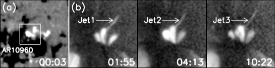
Figure 1: General appearance of the jet region in SOHO MDI magnetogram (a) and the three recurring jets in Hinode XRT SXR images (b). The field of view (FOV) is 135${\times}$135.

On 2007 June 5, the NOAA AR 10960 (S08E29) held a very complex configuration of $\beta$$\gamma$$\delta$-type and was gradually decaying. It is found that there were many coronal jets ejecting from the north of its westernmost sunspot. Here, we mainly examined three of them, which were simultaneously observed by EUV and SXR wavelengths. Figure 1 shows the general appearance of the three recurring jets on SXR images and their location on MDI magnetogram. The NOAA AR 10960 was located at the lower left corner of these images. It is noted that the three jets ejected with bright, nearly collimated morphological structures from the same region, which showed up as point like features on SXR images. Such kind of footpoint was classified to XBP type by Shimojo et al. (1996). They also pointed out that jets from XBPs in ARs tended to appear at the western edge of preceding sunspots, while our three jets appeared at the north edge of preceding sunspot. From the magnetogram, we found that these recurring jets located on a mixed polarities region (marked by white box), which was consistent with the result from Shimojo et al. (1998) that the XBP-like structures at the jet bases were generally rooted in the mixed or satellite magnetic polarities region. In the following section, we demonstrate that magnetic emergences and cancellations take place in this region.

3.1 EUV and SXR jets

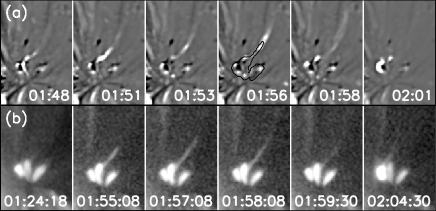
Figure 2: STEREO EUVI 171 Å difference (a) and Hinode XRT SXR direct (b) images showing the evolution of the first jet. In a, all of the images are subtracted by the 00:06 UT image. The black contour plots the soft X-ray jet at 01:57:08 UT. The FOV is 110${\times}$160.

In order to explore morphological and kinetic relationships between EUV and SXR jets, we present evolutions of the three EUV and SXR jets in figure 2-4. Figure 2 shows evolutions of the first jet. In this event, STEREO EUVI 171 Å difference images were used to show EUV jet more clearly. In EUV wavelength (Fig. 2a), we can see a bright, linear jet structure ejected from a bright footpoint. It stretched to the northwest with a converging shape. This jet lasted for about 13 minutes (01:48-02:01 UT), and got the maximum length of 8.1${\times}$10⁴ km at 01:58 UT. We estimated its velocity to be about 135 km s^-1. At the jet base, we observed a very weak brightening, i.e., a small flare. It was a common characteristic of jets and was called subflare or microflare. We note that SXR observations (Fig. 2b) also revealed a bright jet structure with a converging shape. Unfortunately, the XRT observation missed the initial stage of the event due to a data gap (01:24:18-01:55:08 UT). We found that SXR jet also reached the maximum length at 01:58 UT, and its maximum length was about 8.3${\times}$10⁴ km. If we assumed that the SXR and EUV jets had the same start time, then the velocity of the SXR jet was about 138 km s^-1. In addition, the SXR jet at 01:57:08 UT was superposed on the EUV image at 01:56 UT. It is clear that the SXR and EUV jets had the same locations and directions.

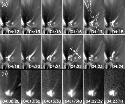
Figure 3: TRACE 171 Å (a) and Hinode XRT SXR (b) direct images showing the evolution of the second jet. The white contour plots the soft X-ray jet at 04:17:40 UT. The FOV is 126${\times}$200.

Evolutions of the second jet were shown in figure 3. In this case, TRACE 171 Å images were used. This event was poorly observed by Hinode XRT SXR observations, and lost data from 04:08:20 to 04:11:13 UT and from 04:17:40 to 04:20:33 UT. Unlike the first jet, its accompanied small flare appeared to be more glaring and its structure seemed to be more complicated. In figure 3a, the EUV jet looked like a single thread before 04:21 UT, while it divided into two threads (marked A and B) after 04:21 UT. Such a bifurcation structure might result from the jet rotation, but we could not identify such rotation from these EUV images. It is noted that such bifurcation could also be seen clearly on the SXR image at 04:22 UT. The EUV jet started at 04:13 UT, reached to the maximum length of 8.7${\times}$10⁴ km at 04:21 UT and completely disappear at 04:24 UT. Its velocity was calculated to be 145 km s^-1. However, due to data gaps, the corresponding SXR jet lost its start time and the time when it elongated to the maximum length. Therefore, we could not give the size and velocity of the SXR jet. We also superposed the SXR jet at 04:17:40 UT on the EUV image at 04:17 UT. As a result, we found that the SXR and EUV jets had the same locations and directions.

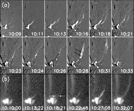
Figure 4: STEREO EUVI 171 Å difference (a) and Hinode XRT SXR direct (b) images showing the evolution of the third jet. In a, all of the images are subtracted by the 10:01 UT image. The black contour plot the soft X-ray jet at 10:27:08 UT. The FOV is 120${\times}$200.

Different from the above two events, the third case contained two jets. In figure 4a, we found that a bright elongated jet first appeared at 10:11 UT. At around 10:12 UT, another jet below it ejected from the jet base. Then, they propagated outward together. At 10:18 UT, the second jet reached to the maximum length of 9.0${\times}$10⁴ km, then quickly faded away and completely disappeared at about 10:23 UT. We estimated its velocity to be about 201 km s^-1. Nevertheless, the first jet got its maximum length of 1.3 ${\times}$ 10⁵ km at 10:31 UT. The velocity of the first jet was about 140 km s^-1. An interesting finding is that the jet at 10:28 UT had two knots (marked by two white arrows), which might indicate that the EUV jet had a twisted structure. The subsequent bifurcation was clearly seen at 10:31 UT. It completely disappeared after 10:33 UT. We also found two jets (marked by two white arrows in figure 4b) in SXR. However, the SXR observations also had many data gaps (10:13:22-10:18:21 UT, 10:18:41-10:22:48 UT and 10:27:08-10:32:07 UT.). Due to these data gaps, we could not calculate the maximum length and velocity of the second jet. If we assumed that the first jet got the maximum lengths of 1.4 ${\times}$ 10⁵ km at 10:32 UT, then its velocity was estimated to be 144 km s^-1. We could not identify the twisted structure and subsequent bifurcation on SXR images. Like the above two events, We superposed the SXR jet at 10:27 UT on the EUV image at 10:26 UT. It is found that the SXR and EUV jets had the same locations and directions.

3.2 Spectral characteristics

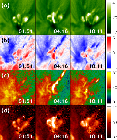
Figure 5: Hinode EIS Fexii $\lambda$195 Å intensity (a), Doppler velocity (b), non-thermal velocity (c), and density (d) maps showing the three recurring jets. The FOV is 110${\times}$110.

The three jets mentioned above were also observed by Hinode EIS, and their spectral characteristics were obtained. Figure 5 shows Fexii $\lambda$195 Å intensity, Doppler velocity, non-thermal velocity, and density maps of the three recurring jets. The Fexii $\lambda$195 Å line has the maximum ionization temperature, i.e., the formation temperature, of 1.3 MK. From intensity maps, three faint elongated jet structures were identified. In the Doppler velocity maps, we note blue-shifted features stretched above red-shifted features at footpoint regions. Clearly, the blue-shifted features were corresponding to the three jets. Maximum blue-shifted velocities and red-shifted velocities for the three jets were calculated. Maximum blue-shifted velocities were 25, 121 and 43 km s^-1 and maximum red-shifted velocities were 11, 38 and 35 km s^-1. We also found non-thermal velocities for the three jets and their footpoint regions. Maximum non-thermal velocities associated with the three jets were 98, 181 and 98 km s^-1, and maximum non-thermal velocities associated with footpoint regions were 90, 130 and 90 km s^-1. Moreover, we also estimated the maximum densities for the three jets, and the values were 2.6${\times}$ 10¹⁰, 3.4${\times}$ 10¹⁰ and 6.6${\times}$ 10⁹ cm^-3. In addition, the three jets could be simultaneously observed by the six spectral lines listed in Table 1. Therefore, we considered that the three jets had temperatures ranged from 0.05 to 2.0 MK.

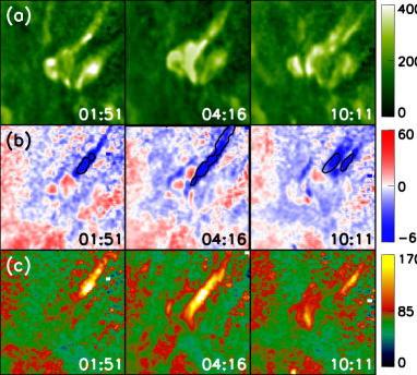
Figure 6: Hinode EIS Heii $\lambda$256 Å intensity (a), Doppler velocity (b), and non-thermal velocity (c) maps showing the three recurring jets. The three black contours outline the three jets in Fexii $\lambda$195 Å velocity maps. The FOV is 110${\times}$110.

We present the spectral characteristics of the three recurring jets obtained by Heii $\lambda$256 Å line (figure 6) to compare with those obtained by Fexii $\lambda$195 Å line. The Heii $\lambda$256 Å line formed at a temperature of 0.05 MK. The three jets in the intensity maps given by Heii $\lambda$256 Å line appeared to be more powerful than that given by Fexii $\lambda$195 Å line. We found blue-shifted features related to the three jets and red-shifted features associated with their footpoint regions. Their maximum blue-shifted velocities were 229, 232, and 115 km s^-1, and maximum red-shifted velocities were 21, 28, and 35 km s^-1. Maximum non-thermal velocities associated with the three jets were 399, 336 and 196 km s^-1, while maximum non-thermal velocities associated with the footpoint regions were 113, 263 and 155 km s^-1. Apparently, maximum blue-shifted and non-thermal velocities associated with the three jets calculated in Heii $\lambda$256 Å line were higher than those calculated in Fexii $\lambda$195 Å.

Figure 7: The maximum ionization temperature dependence of the Doppler velocity in the three jets averaged over the white boxes marked in Fig. 5. The error bars represent the corresponding fitting errors.

Using six emission line listed in table 1, we investigated the relations of averaged Doppler velocities and maximum ionization temperatures for the three jets. For each jet, averaged Doppler velocities were calculated in the white box in Figure 5 and these relations for the three jets were shown in figure 7. We found that the three jets had a common tendency: averaged Doppler velocities decreased with the increase of the maximum ionization temperature. Meanwhile, we superposed blue-shifted feature corresponding to the three jets in Fexii $\lambda$195 Å Doppler velocity maps on Hexii $\lambda$256 Å Doppler velocity maps (see figure 6b) and found that the blue-shifted area also decreased with the increase of the maximum ionization, which was consistent with the result given by Kim et al. (2007). According to these observational results, we infer that magnetic reconnection associated with these recurring jets take place at the lower transition region or chromosphere, i.e., low temperature region.

3.3 Evolutions of longitudinal magnetic fields

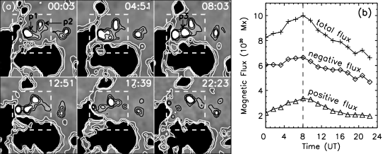
Figure 8: (a) Time sequences of SOHO MDI magnetograms superposed by iso-gauss contours with levels $\pm$50, $\pm$100 and $\pm$150G. White boxes indicate the base of these recurring jets. (b) Evolutions of positive, negative and total magnetic fluxes in white boxes of this figure. The FOV is 80${\times}$80. The dashed vertical bar represent the time boundary of the increase and decrease of the magnetic flux.

The magnetic field evolution at the base of these recurring jets (marked by white boxes) was shown in figure 8a. The positive and negative polarities were represented by white and dark colors, respectively. For clearly exhibiting the magnetic field evolution, we superposed iso-gauss contours with levels $\pm$50, $\pm$100 and $\pm$150G on these magnetograms. We note two emerging magnetic features, ”p1” and ”p2”, at the jet base in the 00:03 UT frame. Before 08:03 UT, their area continuously increased, indicating that new magnetic flux emerged into this region. Meanwhile, these emerging magnetic features moved southeastward, then squeezed and cancelled with their surrounding negative magnetic flux. At 08:03 UT, the positive magnetic flux got the maximum area and another emerging magnetic feature, ”p3”, between p1 and p2 were identified, while the negative magnetic flux east of them clearly decreased. After 08:03 UT, the positive magnetic flux and their surrounding negative magnetic flux apparently decreased. At 22:23 UT, p1 and p3 almost disappeared completely.

We also calculated the positive, negative and total magnetic fluxes in white boxes of Figure 8a and showed their evolutions in figure 8b. It is obvious that the opposite magnetic flux increased asymmetrically before 08:03 UT, with positive magnetic flux increased largely whereas the negative magnetic flux increased slightly. According to our calculation, average flux-gain rates of the positive flux and the negative flux were 4.0 ${\times}$ 10¹⁵ Mx s^-1 and 2.0 ${\times}$ 10¹⁵ Mx s^-1, respectively. After 08:03 UT, the decrease of the opposite magnetic flux also show an asymmetry, and flux-loss rates of the negative magnetic flux and the positive magnetic flux were 3.8 ${\times}$ 10¹⁵ Mx s^-1 and 2.7 ${\times}$ 10¹⁵ Mx s^-1, respectively. For the asymmetry before 08:03 UT, it might be the result that the negative polarity of the emerging bipole was out of the field marked by white boxes. The asymmetry after 08:03 UT can be interpreted as part of negative magnetic flux moving out the white boxes. As a result, the total magnetic flux had a averaged flux-gain rate, 6.1 ${\times}$ 10¹⁵ Mx s^-1, and a averaged flux-loss rate of 6.6 ${\times}$ 10¹⁵ Mx s^-1. According to Shimojo et al. (1998), the difference between the observed increase or decrease in the flux of the jet-producing region was resulted from the difference in the rates of the magnetic flux emergence and photospheric reconnection. Furthermore, we found that these recurring jets occurred not only when total magnetic flux was increasing, but also when it was decreasing, which was similar to observations of Shimojo et al. (1998).

4 Conclusions and discussions

In this paper, we compared three EUV and SXR jets and analyzed their spectral properties, and the main observational results are summarized as follows: (1) These recurring jets were located on a mixed polarities region near a sunspot, and clear magnetic flux emergence and cancellation occurred at their location. (2) These EUV and SXR jets ejected from the same site, and had similar directions, sizes and velocities. The third EUV jet showed an apparent helical structure, but this structure could not be resolved on SXR images. (3) These three jets had temperatures from 0.05 to 2.0 MK and maximum electron densities from 6.6$\times$10⁹ cm^-3 to 3.4 $\times$10¹⁰ cm^-3. (4) Elongated blue-shifted features associated with jets and red-shifted features at the jet bases were simultaneously observed in Fexii $\lambda$195 and Heii $\lambda$256 lines. (5) In Fexii $\lambda$195, the three jets had maximum Doppler velocities from 25 km s^-1 to 121 km s^-1 and maximum non-thermal velocities from 98 km s^-1 to 181 km s^-1; the jet bases had maximum Doppler velocities from 11 to 35 km s ^-1 and the maximum non-thermal velocity from 90 to 130 km s^-1. (6) In Heii $\lambda$256, maximum Doppler velocities and maximum non-thermal velocities of the three jets were from 115 to 232 km s^-1 and from 196 to 399 km s^-1, respectively; maximum Doppler velocities and maximum non-thermal velocities at the jet bases were from 21 to 35 km s ^-1 and from 113 to 263 km s^-1, respectively. (7) averaged Doppler velocities associated with jets decreased with the increase of maximum ionization temperatures.

We compared EUV and SXR jets in an AR, and found that they had similar sizes and velocities. These observational results were consistent with Kim et al. (2007), who discovered that EUV and SXR jets had similar characteristics in terms of projected speed, size and lifetime. However, these characteristics were different from Chae et al. (1999). In their work, the EUV jet had a typical size of 4000-10000km, a transverse velocity of 50-100km s^-1, and a lifetime of 2-4 minutes, smaller and shorter lived than X-ray jets. According to Kim et al. (2007), these differences were probably caused by the different locations of the reconnection points. Magnetic reconnections related to our investigated recurring jets might take place at more higher solar atmosphere than those studied by Kim et al. (2007). In addition, one of the three EUV jets implied a helical structure, while the corresponding SXR jet did not. The differences in morphology between EUV and SXR jets were ever reported by Alexander & Fletcher (1999), Kim et al. (2007) and Chifor et al. (2008b). Alexander & Fletcher (1999) pointed out that EUV jets had twisted structures, Kim et al. (2007) demonstrated multi-structures in EUV jets, while Chifor et al. (2008b) observed expanding loops associated with X-ray jets instead of EUV jets.

For the three jets, their corresponding Doppler velocity maps from EIS revealed apparent blue-shifted features elongated from red-shifted bright points. We interpreted them as jets because all of them were transient. Their maximum Doppler velocities were calculated and it is found that all the derived values were lower than that given by Chifor et al. (2008a), who showed that the upflow velocities associated with an active region jet exceeded 150 km s^-1. In addition, the maximum Doppler velocity obtained by Heii 256.320 line could reach to 232 km s^-1, which was much larger than 62 km s^-1 estimated by Kim et al. (2007). Moreover, We examined the relationship between the averaged Doppler velocity and the maximum ionized temperature near the jet base, and noted that the averaged Doppler velocity decreased with the increase of the maximum ionized temperature. According to this observation, we assumed that magnetic reconnections associated with these three jets might occur in the low-temperature region, i.e., the higher chromosphere or the lower transition region. Kim et al. (2007) simultaneously found blue-shifted and red-shifted motions at the jet base. Different from them, we only observed red-shifted features at the jet base, which were similar to the observations of Kamio et al. (2007) and Chifor et al. (2008b). Because evaporation flow was considered to be an upflow at the coronal temperature, this phenomenon was not consistent with the evaporation scenario (Kamio et al., 2007). We regarded this kind of red-shifted feature as downflows in reconnected flares, downward reconnected loops, or downward streams of bi-directional reconnection outflows.

In this work, obvious magnetic flux emergences and cancellations induced these recurring jets. Such instances were ever reported by Chae et al. (1999), Zhang et al. (2000), Liu & Kurokawa (2004), and Jiang et al. (2007). Recently, Archontiset al. (2010) proposed a 3D numerical simulation, in which a toroidal flux tube emerged into the solar atmosphere and interacted with a pre-existing field of an AR. In their simulation, recurrent coronal jets were produced. They thought that the emergence of new magnetic flux introduced a perturbation to the AR, and caused reconnection between neighboring magnetic fields and the release of the trapped energy in the form of jet-like emissions. Moreover, they also pointed out that when the amount of emerging flux was exhausted, the dynamic rise slowed down and reached an equilibrium. In our case, magnetic emergences first dominated the jet base, the amount of them reached to the maximum at 08:03 UT. Then they began to decay, and their associated jet activities decreased. At 22:23 UT, emerging magnetic features p1 and p3 almost completely disappeared. After 22:23 UT, we could not observed one clear jet activity. These observations strongly support the simulation results given by Archontiset al. (2010).