Lanchester Theory and the Fate of Armed Revolts

Abstract

Major revolts have recently erupted in parts of the Middle East with substantial international repercussions. Predicting, coping with and winning those revolts have become a grave problem for many regimes and for world powers. We propose a new model of such revolts that describes their evolution by building on the classic Lanchester theory of combat. The model accounts for the split in the population between those loyal to the regime and those favoring the rebels. We show that, contrary to classical Lanchesterian insights regarding traditional force-on-force engagements, the outcome of a revolt is independent of the initial force sizes; it only depends on the fraction of the population supporting each side and their combat effectiveness. We also consider the effects of foreign intervention and of shifting loyalties of the two populations during the conflict. The model’s predictions are consistent with the situations currently observed in Afghanistan, Libya and Syria (Spring 2011) and it offers tentative guidance on policy.

1 Introduction

Recent (2011) events in Libya underscore the significant impact of armed revolts on regional and global interests. Armed revolts typically start with demonstrations and civic unrest that quickly turn into local violence and then full-scale combat. (The terms revolt, rebellion, and insurgency are interchangeable in most senses and we use the term revolt throughout for consistency.) As demonstrated in Libya the evolution of the armed revolt has a strong spatial component; individuals in some regions (e.g., parts of Tripoli) may be loyal to the regime because of ideology or economic and social incentives or fear, while other regions (e.g., Benghazi) become bastions of the rebels powered by strong local popular support. Thus, armed revolts, very much like conventional war, are about gaining and controlling populated territory. However, unlike conventional force-on-force engagements, where the civilian population plays a background role, armed revolts are characterized by the active role of the people, who become a major factor in determining the outcome of the conflict: both the rebels and the regime need the support of the population to carry out their campaigns [3, 4, 6].

Our approach to modeling armed revolts is based on Lanchester theory [5] that describes the strength of two opposing military forces by two ordinary differential equations (ODEs). The forces cause mutual attrition that depletes their strengths until one of the forces is defeated. While Lanchester models are stylized and highly abstract, they have been extensively used for analysis for almost a century because they provide profound insights regarding conditions that affect the outcomes of military conflicts [11].

Using our model, we derive the end-state of the revolt, identify stalemate situations and study the effects of foreign intervention and of inconstant support by the population. We show that contrary to classical Lanchesterian insights regarding traditional force-on-force engagements, the outcome of a revolt is independent of the initial force sizes. We also derive conditions for successful foreign interventions. These results are consistent with the situations currently (Spring 2011) observed in Afghanistan, Libya and Syria. We also evaluate policy options facing the international community.

2 Setting and Assumptions

Consider an armed revolt involving two forces, termed Red and Blue, that rely on the population for manpower, intelligence, and most other resources. The population is divided into supporters of the Blue, called henceforth supporters, and supporters of Red, called henceforth contrarians. We initially assume that the support strongly depends on factors such as tribal affiliation, social class, and ideology and therefore remains unchanged during the armed revolt. However, later on we relax this assumption and allow for changes in popular behavior, reflecting pragmatic and opportunistic responses of the population to changes in the force balance.

We assume that the country is divided between Red and Blue and therefore a populated region lost by one force is gained by the other force. A force that fights over a region might be either supported or opposed by the local population, situations which we call liberation or subjugation, respectively. A liberating force fights more effectively than a subjugating force because of population support, ceteris paribus. Moreover, the forces in control of hostile regions are busy policing the population and therefore adopt a defensive posture. Thus, only the forces operating in friendly regions proactively attempt to capture additional territories.

3 Model

Let $S$ and $C$ ($S+C=1$) denote the fraction of the total population who are supporters of Blue and supporters of Red (“contrarians”), respectively. Let also $B$ and $R$ ($B+R=1$) denote the fraction of the population controlled by Blue and Red, respectively. We use the notation $XY$ for the fraction of population $X$ that is controlled by force $Y$, where $X=S,C$ and $Y=B,R$. Hence, $SB+SR=S$ and $CB+CR=C$. When Blue subjugates a $CR$ region it becomes part of $CB$ and when Blue liberates an $SR$ area it becomes part of $SB$. Similar actions are possible by Red, giving a total of four kinds of combat engagements, as shown in Figure 1.

Because Red and Blue operate in populated areas, the outcome of an engagement depends both on the strength of the attacking force but also on the signature (i.e. visibility) of the defending force; smaller attack force (“fewer shooters”) or smaller signature (“fewer targets”) result in a smaller gain/loss rate. Namely, at each interaction, the gain rate of the attacker is given by a scaling constant, called henceforth attrition rate, multiplied by the product of the attacking and defending force sizes. This relationship implies that even a large attacker would struggle to suppress a small defender diffused in the population. The resulting model is an adaptation of the Lanchester Linear Law (see e.g., [11] p. 83) and Deitchman’s guerrilla warfare model [2].

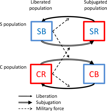
Figure 1: Schematic dynamics of the model. The four variables in the model appear as boxes, where each box represents a possible combination of population behavior and controlling force. Solid lines indicate change in control of population while dashed lines indicate the force causing it. Observe that the population does not change allegiances even under occupation.

The attrition rate constants depend on the tactics and equipment of the parties as well as the behavior of the population. Thus, let $f_{S}$ and $f_{C}$ denote the rates of liberation of friendly regions by Blue and Red forces, respectively. Similarly, let $h_{C}$ and $h_{S}$ denote the rates of subjugation of hostile regions by Blue and Red, respectively. The resulting dynamics are given in Eqs. 1.

$$SB^{\prime} =+f_{S}SB\cdot SR-h_{S}CR\cdot SB$$

$$SR^{\prime} =-f_{S}SB\cdot SR+h_{S}CR\cdot SB$$ (1)

$$CR^{\prime} =+f_{C}CR\cdot CB-h_{C}SB\cdot CR$$

$$CB^{\prime} =-f_{C}CR\cdot CB+h_{C}SB\cdot CR$$

Since it is easier to fight in friendly territory, we make the following dominance assumption:

$$f_{S}>h_{C}\mbox{ and }f_{C}>h_{S}\,.$$ (2)

4 End-State of the Revolt

From solving Eqs. 1 we obtain that the conflict can result in one of three outcomes, corresponding to the stable equilibrium points of the equations:

1. Blue victory: $SB+CB=1$,

2. Red victory: $CR+SR=1$,

3. Stalemate: Both sides control a fraction of the total population.

It can be shown that the evolution of the conflict does not involve cycles where populated regions change sides endlessly; rather, the conflict dissipates and reaches a stable state (proofs of this and all other results are given in the Supporting Information at the end of this article.)

The stable outcomes are not dependent on all four attrition rates but rather on two ratios: $r_{S}=\frac{f_{S}}{h_{S}}$ and $r_{C}=\frac{f_{C}}{h_{C}}$. We call these the “liberation-subjugation effectiveness ratio” (LSER) of supporters and contrarians, respectively. These ratios account for differences in tactics, technology, and information between Blue and Red, and also reflect the ability and commitment of the local population to support its preferred force. The outcomes are:

Blue wins if and only if $$\qquad r_{C}<\frac{S}{1-S}$$ (3)

Red wins if and only if $$\qquad r_{S}<\frac{1-S}{S}$$ (4)

Stalemate occurs otherwise.

These results are summarized in Figure 2(left). It follows from Ineqs. 3–4 that the fate of the armed revolt is completely determined by the LSERs and the population split between supporters $S$ and contrarians $C=1-S$; it does not depend on the initial sizes of the Blue and Red forces. Moreover, the minimum popular support needed to guarantee Blue’s win only depends on the LSER in the contrarians’ territory. Specifically, Blue wins if and only if $r_{C}(1-S)<S,$ that is, if the fraction of its supporters is larger than the fraction of contrarians times the LSER in contrarians’ territory. An equivalent statement applies for Red victory, which happens if and only if $r_{S}(1-C)<C$. The operational implication of these two conditions is that strengthening one’s advantage in friendly territories (e.g., Blue increasing $r_{S}$) may be sufficient to avoid defeat but not to secure a win; if one is not effectively fighting in hostile territory (e.g., Blue cannot sufficiently decrease $r_{C}$) then one cannot win; the best it can hope for is a stalemate. At the stalemate equilibrium, denoted $XY_{b}$

$$CB_{b} =\frac{S(1+r_{S})-1}{r_{S}r_{C}-1}, SR_{b} =\frac{r_{C}-S(1+r_{C})}{r_{S}r_{C}-1},$$ (5)

$$SB_{b} =r_{C}CB_{b}, CR_{b} =r_{S}SR_{b}.$$

Notice that the denominators are always positive because of the dominance assumption (see Ineqs. 2). Eqs. 5 indicate that as $S$ increases an increasing part of the population is controlled by Blue. When $r_{C}$ increases, a larger fraction of the contrarians is able to remain free (i.e. ruled by Red).

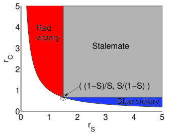
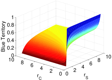
Figure 2: Outcomes of the conflict when $S=40\%$ as a function of $r_{S}$ and $r_{C}$. (left) The possible outcomes are: stalemate (gray), Red victory (red) and Blue victory (blue). The white area is excluded by the dominance assumption (Ineqs. 2). Outright victory is possible only when one party has a low LSER. Increasing $r_{S}$ and $r_{C}$ makes both parties much more entrenched in their areas, leading to a stalemate regardless of the value of $S$. (right) The amount of territory controlled by Blue. Observe that a very sharp change in the outcome is predicted as $r_{C}$ approaches $\frac{2}{3}$, from a balanced stalemate to a Blue victory.

We plot the fraction of the population controlled by Blue during a stalemate (i.e., $CB+SB$) in Figure 2(right). (We only present the plot for $S=0.4$, but other values of $S$ are qualitatively similar.) Near the Blue victory condition defined by Ineq. 3 the fraction of the population controlled by Blue is near one, but quickly decreases as $r_{C}$ increases. Similarly, the fraction of population controlled by Blue rapidly increases as $r_{S}$ moves away from the Red victory condition. However, after the significant initial change in the fraction of Blue’s regions as $r_{S}$ or $r_{C}$ increases, the surface flattens out. As both $r_{S}$ and $r_{C}$ continue to increase, the fraction of Blue’s regions approaches $S$. Therefore, when $r_{S}$ and $r_{C}$ are reasonably bounded away from their thresholds, an entrenched stalemate occurs where Red and Blue control primarily their friendly territories.

5 Extensions of the Basic model

We consider now two extensions of the basic model: the case of foreign intervention and the case of shifting popular support.

5.1 Foreign Military Intervention

Most large revolts in modern times involved foreign military interventions by regional or global powers [8, 9]. Such interventions can be manifested in two ways: direct and indirect. Direct intervention (e.g., air-strike support to ground units, such as the intervention of NATO forces in Libya in 2011) allows the supported side to exercise more firepower against its opponent. Indirect intervention provides the supported side with force multipliers such as intelligence, training, logistical support and advanced weapons, but no additional firepower per se. In both cases we assume that just one side, say Blue, receives the foreign support. We leave for future studies to consider the case of foreign support to both sides.

Direct intervention.

For simplicity, suppose that the foreign constituent is tactically superior and it experiences negligible attrition (e.g., air support for Blue that is subject to ineffective air defense of Red). Therefore, the effectiveness of the foreign constituent remains fixed throughout the armed revolt. However, similarly to the direct engagements discussed above, its ability to target Red diminishes as the size of Red’s forces decreases. In that case, Red targets are harder to find and engage. Let $\lambda_{S},\lambda_{C}>0$ denote the combat power of the foreign constituent when operating in supporters’ $(S)$ regions and contrarians’ $(C)$ regions, respectively. The separation into two combat power parameters allow for the possibility that the foreign constituent only contributes to certain kinds of operations (e.g. only to liberating supporters), and/or is affected by the behavior of the population, just like Blue. In this case Eqs. 1 become

$$SB^{\prime} =+f_{S}SB\cdot SR-h_{S}CR\cdot SB+\lambda_{S}SR$$

$$SR^{\prime} =-f_{S}SB\cdot SR+h_{S}CR\cdot SB-\lambda_{S}SR$$ (6)

$$CR^{\prime} =+f_{C}CR\cdot CB-h_{C}SB\cdot CR-\lambda_{C}CR$$

$$CB^{\prime} =-f_{C}CR\cdot CB+h_{C}SB\cdot CR+\lambda_{C}CR$$

Since the effectiveness of the foreign constituent remains unaffected, it is clear that Red cannot win. The only two outcomes are Blue’s victory and a stalemate. Blue wins if and only if $\lambda_{C}>f_{C}(1-S)-h_{C}S.$ Otherwise, the armed revolt ends in a stalemate. Like in the basic model, the conflict dissipates and reaches a stable state, and no cycles are possible.

An interesting observation is that the value of $\lambda_{S}$ – the combat power of the foreign constituent in friendly regions – plays no role in helping Blue achieve victory; it only ensures that Blue will not lose as long as $\lambda_{S}>0$. The threshold of $\lambda_{C}$ that determines Blue’s victory is the difference between two terms, each a combination of combat effectiveness and popular support: $f_{C}(1-S)$ is Red’s effectiveness fighting on friendly territory times its popular support, and $h_{C}S$ is Blue’s effectiveness fighting on hostile territory times its popular support. Clearly, this threshold decreases as the support to Blue increases. In particular, a sufficient condition for Blue victory is $\lambda_{C}>f_{C}$, which only depends upon the fighting effectiveness of Red. Consequently, even if Blue has limited tactical capabilities or a small amount of popular support, it can still prevail with enough assistance from a foreign constituent.

Indirect intervention.

Indirect intervention (force multiplier) increases the ability of Blue to defend its territory and to attack Red forces. Specifically, the liberation rate $f_{S}$ and the subjugation rate $h_{C}$ are multiplied by factors $\mu_{S},\mu_{C}>1$, respectively, where the structure of Eqs. 1 remains unchanged. The LSER values $r_{S}$ and $r_{C}$ change to $\mu_{S}r_{S}$ and $\frac{r_{C}}{\mu_{C}}$, respectively. Using the conditions in Ineq. 4 we obtain that for Blue to avoid defeat it is sufficient that the intervention be such that:

$$\mu_{S}\geq\frac{1-S}{r_{S}S}.$$

In order to secure a win, it follows from Ineq. 3 that the support for Blue must be such that

$$\mu_{C}>\frac{r_{C}(1-S)}{S}.$$

Because $r_{S}r_{C}>1$, the threshold of $\mu_{C}$ is always larger than the threshold of $\mu_{S}$ – it is more costly to secure a victory than to avoid a loss. Obviously, the indirect intervention is needed to secure a victory only if $S$ is small enough, specifically, if $S<\frac{r_{C}}{1+r_{C}}.$ Note that “small enough” may actually be quite large when Red is very effective on its own turf compared with Blue ($r_{C}$ is large).

5.2 Opportunistic Population

While in some conflicts the behavior of the people is highly polarized and unchanging, in others the population might be quite opportunistic and favor the side that appears more likely to win. It follows that the fraction of the supporters, and hence contrarians, changes according to the state of the conflict. We capture this situation by treating the fraction of supporters $S$ as a dynamic variable, and adding to Eqs. 1 an equation for $S^{\prime}$. The value of $S^{\prime}$ increases with the fraction of population Blue controls ($SB+CB$) and decreases with the fraction controlled by Red ($CR+SR$). Because $C=1-S$, $SR=S-SB$, and $CB=1-S-CR$, we obtain from Eqs. 1 the three independent equations:

$$SB^{\prime} =+f_{S}SB(S-SB)-h_{S}CR\cdot SB$$

$$CR^{\prime} =+f_{C}CR(1-S-CR)-h_{C}SB\cdot CR$$ (7)

$$S^{\prime} =+\alpha(SB+1-S-CR)(1-S)-\alpha(CR+S-SB)S,$$

where $\alpha$ is a parameter that determines the rate at which individuals switch allegiances, which is assumed to be the same for both the supporters and contrarians. With opportunistic population there are only two potential outcomes:

1. Blue victory where the entire population supports Blue, who controls all regions ($SB=1$), and

2. Red victory where the entire population supports Red, who controls all regions ($CR=1$).

These two equilibria are stable for all parameter values. There are also two stalemate equilibria: a balanced stalemate where $SB,CR>0$, and a disarmed stalemate where $SB=CR=0$. Neither of the two stalemate equilibria are stable. The disarmed stalemate is neither realistic nor relevant. The balanced stalemate, given below, is more interesting because it lies on a boundary that separates the basins of attraction for the two victory situations:

$$SB^{\ast} =\frac{r_{C}}{2+r_{S}+r_{C}},$$ (8)

$$CR^{\ast} =\frac{r_{S}}{2+r_{S}+r_{C}},$$ (9)

$$S^{\ast} =\frac{1+r_{C}}{2+r_{S}+r_{C}}.$$ (10)

Thus, the stalemate equilibrium gives a rough metric for the potential outcome of the conflict. For example, the closer the stalemate equilibrium is to the Blue victory point, the more likely Red will win the conflict. This occurs because most of the 3-dimensional $(r_{S},r_{C},S)$ parameter space lies in the basin of attraction corresponding to Red victory.

6 Discussion of Some Armed Revolts

Using the results above, we analyze several ongoing (in 2011) revolts. While we could not access reliable data to empirically validate our model (e.g., estimates of LSERs $r_{S}$ and $r_{C}$ or time-series data of conflicts), we show that many of the ongoing conflicts are at a state consistent with our model. The model suggests how their outcomes might be effected by decisions including those currently on the policy table.

Libya

The available information regarding the revolt in Libya is based mainly on fragmented news reports. As of June 2011, it appears that at least three of the seven largest districts in Libya – Benghazi, Misrata and Az-Zawiya – support the rebels, which amount to at least $40\%$ of the population. The Qaddafi forces (labeled Red) are much better trained, equipped and organized than the rebels (labeled Blue). Therefore, if $S$ denotes the supporters of the rebels, it is reasonable to assume that $f_{S}<h_{S}$ and $f_{C}>h_{C}$ – the regime forces have the upper hand even in hostile regions, which implies that $r_{S}<1$ and $r_{C}>1.$ Ineq. 4 suggests that Qaddafi should have achieved a clear victory, crushing the revolt. Indeed, he appeared to be nearing victory until the intervention of NATO forces that implemented a no-fly zone and later launched a series of air-strikes against Qaddafi’s forces. In our terminology, NATO forces have applied direct intervention. This intervention, if sustained, implies that the rebels now cannot be defeated. From news reports it appears that the rebels have also been provided training and gear to help them repel Qaddafi’s attempts at recapturing rebelling population, i.e. increasing the rebels’ $r_{S}$. At the same time, the rebels have been unable to make inroads into territory currently controlled by Qaddafi, so $r_{C}$ is largely unchanged. Under those conditions the model suggests that the most likely outcome is a protracted stalemate. To achieve victory for the rebels, the foreign intervention must focus on decreasing $r_{C}$ and/or increasing $\lambda_{C}$, that is, attack or help attack the regions supporting the regime.

Afghanistan

One can view the ongoing conflict in Afghanistan (2001-) as a struggle of government and coalition forces (Blue) against Salafists (Red) led by the Taliban. Many observers of the conflict point to the critical need of both parties to win the support of the population, so the conflict is a good application of our model. According to the 2007 report by the International Council on Security and Development, the Taliban have permanent presence in 54% of the country [7]. Suppose, pessimistically, that the Taliban movement has the support of all the people in the regions where it is present. Assuming fixed behavior of the population (no opportunistic shifts) the situation in Afghanistan will continue in its current stalemate form unless $r_{S}<1.17$ (giving Red a victory) or $r_{C}<0.85$ (giving Blue a victory). Thus, the model suggests that the government can avoid a Taliban takeover of the country by nurturing the support of the population it currently controls, and it is not necessary to push back the Taliban from their areas.

Syria

The civil unrest in Syria currently pits the Syrian army and paramilitaries against massive but unarmed demonstrations. If the situation escalates into an armed revolt, what might be its outcome? It would appear that special units of the Syrian army possess superior tactics and weapons sufficient to suppress any domestic military opponent. However, we anticipate the regime to face a strong challenge because of its narrow base of support in the Alawite sect. If we assume that loyalties do not shift, then the rebels (Red) would be victorious against the government (Blue) if $r_{S}<\frac{1-S}{S}$ (Ineq. 4). Assuming $S\approx 10\%$ (the entire Alawite community [1]), the government must have LSER of $r_{S}\geq 9$ to avoid defeat. This seems unlikely given the discontent even within the Alawite community and the ease with which foreign backers of the rebels could provide them with military hardware, such as armor-piercing munitions and air cover to neutralize government forces. The current (June 2011) observed stalemate is a result of small foreign intervention by Iranian and Hezbollah combatants. This intervention is covert and therefore very fragile. Thus, we expect that in an armed revolt along the lines of our model, Syria’s Assad regime would be defeated.

7 Conclusions and Policy Implications

We present a new Lanchester-type model that represents the dynamics of liberating and subjugating populated regions in the setting of an armed revolt. We identify winning and stalemate conditions and obtain some general insights regarding the revolt’s end state. Many revolts do not have a decisive outcome, with both sides entrenched in a prolonged stalemate. Our model explicitly identifies this realistic outcome, which is not captured in classical Lanchester theory. Our model also illustrates that it is not sufficient to ably control friendly regions; for victory it is crucial to be able to effectively fight in hostile regions.

We also study the effect of foreign intervention (e.g., NATO intervention in Libya) on the outcome of a revolt. We find that while direct intervention to support one side will prevent defeat of that side and can facilitate a win even if that side has very little popular support, indirect intervention cannot guarantee this. If the opponent (Red) has strong popular support and the supported force (Blue) has a poor LSER such that $\frac{1-S}{r_{S}S}>1$, then if $1<\mu_{S}<\frac{1-S}{r_{S}S},$ the supported force will actually lose – the indirect support is simply not large enough. The level of foreign intervention (either direct or indirect) required to defeat an opponent depends on the popular support $(S)$ and the attrition coefficients ($f_{C}$ and $h_{C}$) in the contrarians’ territory; it does not depend on the capabilities of the forces in supporters’ regions.

Finally if the population can shift its support, then a stalemate is not possible. A bandwagon-type effect will occur where the population increases its support to the apparent winner, which strengthens it and leads to more support, which further strengthens it and so on until the side achieves victory. Unlike the case of fixed population behavior, the results of this scenario are sensitive to the initial conditions.

8 Supporting Information

We present here the mathematical proofs of the results presented in the main text.

8.1 Victory Conditions

In general, dynamical systems may exhibit stable oscillations. We now show that the system of equations in Eqs. 1 does not have those oscillations (no limit cycles). This means that the state variables will always reach one of the equilibrium points (by the Poincaré-Bendixon Theorem [10]).

Theorem 1 (Dulac’s Criterion [10]).

Let $\dot{x}=f(x)$ be a smooth system on a simply-connected set $S\subset\mathbb{R}^{2}.$ Let $w:S\to\mathbb{R}$ be smooth on $S$. Suppose on $S$ the expression $\nabla\cdot\left(f(x)w(x)\right)$ does not change sign. Then the system has no limit cycle on $S$.

Proposition 1.

The system of Eqs. 1 does not have limit cycles.

Proof.

We first write the model as a system of two independent equations by removing the mixed variables:

$$SB^{\prime} =+f_{S}SB(S-SB)-h_{S}CR\cdot SB$$ (11)

$$CR^{\prime} =+f_{C}CR(C-CR)-h_{C}SB\cdot CR$$ (12)

Let

$$w(SB,CR)=\frac{1}{SB(S-SB)CR(C-CR)}.$$

Both the system and $w$ are smooth on the set $(0,S)\times(0,C)$ (points on the boundary of this space move to one of the fixed points and do not oscillate.)

$$\nabla\cdot\left(fw\right) =\nabla\cdot\left(\frac{f_{S}(S-SB)-h_{S}CR}{(S-SB)CR(C-CR)},\frac{f_{C}(C-CR)-h_{C}SB}{SB(S-SB)(C-CR)}\right)$$

$$=\frac{-h_{S}}{(S-SB)^{2}(C-CR)}+\frac{-h_{C}}{(S-SB)(C-CR)^{2}}<0.$$

∎

We next show that the victory conditions in 3, 4 correspond to the stability conditions for the equilibria points. Throughout, we assume that $0<S<1$, i.e. $S$ is not on its boundary.

Theorem 2.

The following four statements hold for the system of differential equations defined by Eqs. 1:

• The equilibrium $CR=SB=0$ and $SR=1-CB=S$ is never stable.

• The Blue victory equilibrium ($CR=SR=0$ and $SB=1-CB=S$) is stable if and only if $r_{C}<\frac{S}{1-S}$.

• The Red victory equilibrium ($SB=CB=0$ and $CR=1-SB=1-S$) is stable if and only if $r_{S}<\frac{1-S}{S}$.

• The stalemate equilibrium (defined by Eqs. 5)) is stable if and only if $r_{C}\geq\frac{S}{1-S}$ and $r_{S}\geq\frac{1-S}{S}$.

Proof.

The model is fully specified based on two variables: $SB$ and $CR$, Eqs. 11-12. We first compute the Jacobian of the right hand size of differential equation

$$\mathbf{J}(SB,CR)=\begin{pmatrix}f_{S}(S-2SB)-h_{S}CR&-h_{S}SB\\ -h_{C}CR&f_{C}(1-S-2CR)-h_{C}SB\end{pmatrix}$$

A solution $(SB^{*},CR^{*})$ to the differential equation is stable if the two eigenvalues of $\mathbf{J}(SB^{*},CR^{*})$ have negative real parts [10]. By inspection the equilibrium with $SB=CR=0$ is not stable for any parameter values.

Blue Victory
The characteristic polynomial in this case is

$$(-f_{S}S-\lambda)(f_{C}(1-S)-h_{C}S-\lambda)=0\,.$$

The first eigenvalue, $-f_{S}S$, is always negative and the second eigenvalue, $f_{C}(1-S)-h_{C}S$, is negative if $r_{C}<\frac{S}{1-S}$.

Red Victory
The characteristic polynomial in this case is

$$(-f_{C}(1-S)-\lambda)(f_{S}S-h_{S}(1-S)-\lambda)=0\,.$$

The first eigenvalue, $-f_{C}(1-S)$, is always negative and the second eigenvalue, $f_{S}S-h_{S}(1-S)$, is negative if $r_{S}<\frac{1-S}{S}$. By the dominance assumption (i.e., Ineq. 2)) $r_{S}r_{C}>1$ and thus $\frac{1}{1+r_{S}}<\frac{r_{C}}{1+r_{C}}$. Therefore it is not possible for both the Blue victory and Red victory to be stable equilibria for the same values of $r_{S}$ and $r_{C}$. This also implies that if $r_{S}<\frac{1-S}{S}$ a Blue victory cannot occur and if $r_{C}<\frac{S}{1-S}$ a Red victory cannot occur.

Stalemate
At the stalemate equilibrium in section 4, the variables have the values $SB_{b}$, $SR_{b}$, $CR_{b}$, and $CB_{b}$. We next present a lemma, and then prove that the stalemate equilibrium is stable if and only if $\frac{1}{1+r_{S}}<S<\frac{r_{C}}{1+r_{C}}$, which is equivalent to the two conditions $r_{C}\geq\frac{S}{1-S}$ and $r_{S}\geq\frac{1-S}{S}$

Lemma 1.

The product $SB_{b}CR_{b}$ is positive if and only if $\frac{1}{1+r_{S}}<S<\frac{r_{C}}{1+r_{C}}$.

Proof.

By Eqs. 5, $SB_{b}$ is positive if $\frac{1}{1+r_{S}}<S$, and $CR_{b}$ is positive if $S<\frac{r_{C}}{1+r_{C}}$. By the dominance assumption (Ineq. 2) $\frac{1}{1+r_{S}}<\frac{r_{C}}{1+r_{C}}$, and therefore it is impossible for $SB_{b}$ and $CR_{b}$ to both be negative. ∎

Lemma 1 and Eqs. 5 imply that if $\frac{1}{1+r_{S}}<S<\frac{r_{C}}{1+r_{C}}$, then $SB_{b}$, $SR_{b}$, $CR_{b}$, and $CB_{b}$ are all positive (and by conservation of total population, less than 1). The Jacobian matrix for the stalemate equilibrium is

$$\mathbf{J}(SB_{b},CR_{b})=\begin{pmatrix}-f_{S}SB_{b}&-h_{S}SB_{b}\\ -h_{C}CR_{b}&-f_{C}CR_{b}\end{pmatrix}$$

We derive the upper left hand element of this Jacobian below

$$\mathbf{J}_{11}(SB_{b},CR_{b}) =f_{S}(S-2SB_{b})-h_{S}CR_{b}$$

$$=h_{S}(r_{S}(S-2SB_{b})-r_{S}SR_{b})$$

$$=f_{S}\left(S-\frac{2Sr_{C}(1+r_{S})-2r_{C}}{r_{S}r_{C}-1}-\frac{r_{C}-S(1+r_{C})}{r_{S}r_{C}-1}\right)$$

$$=-f_{S}SB_{b}$$

The lower right hand element of $\mathbf{J}(SB_{b},CR_{b})$ can be derived in a similar fashion and we omit the details. The eigenvalues of $\mathbf{J}(SB_{b},CR_{b})$ will both have a negative real component if the trace of $\mathbf{J}(SB_{b},CR_{b})$ is negative and the determinant is positive. The determinant of $\mathbf{J}(SB_{b},CR_{b})$ is $SB_{b}CR_{b}h_{C}h_{S}(r_{S}r_{C}-1)$. If $\frac{1}{1+r_{S}}<S<\frac{r_{C}}{1+r_{C}}$, then by Lemma 1 the trace is negative and the determinant is positive and thus the stalemate equilibrium is stable. If $S\notin\left(\frac{1}{1+r_{S}},\frac{r_{C}}{1+r_{C}}\right)$ then by Lemma 1 the determinant of $\mathbf{J}(SB_{b},CR_{b})$ is negative and thus one of the eigenvalues has a positive real component and the stalemate equilibrium is not stable. ∎

8.2 Direct Foreign Intervention

Let us rewrite the direct intervention dynamics of Eqs. 6:

$$SB^{\prime} =+f_{S}\left(SB+\frac{\lambda_{S}}{f_{S}}\right)SR-h_{S}CR\cdot SB$$

$$SR^{\prime} =-f_{S}\left(SB+\frac{\lambda_{S}}{f_{S}}\right)SR+h_{S}CR\cdot SB$$ (13)

$$CR^{\prime} =+f_{C}CR\cdot CB-h_{C}\left(SB+\frac{\lambda_{C}}{h_{C}}\right)CR$$

$$CB^{\prime} =-f_{C}CR\cdot CB+h_{C}\left(SB+\frac{\lambda_{C}}{h_{C}}\right)CR$$

Furthermore let us define $A_{S}\equiv\frac{\lambda_{S}}{f_{S}}$ and $A_{C}\equiv\frac{\lambda_{C}}{h_{C}}$. The stalemate equilibrium of these equations is denoted with a subscript $fi$ (“foreign intervention”) and we present them below.

$$SB_{fi} =\frac{SB_{b}}{2}-\frac{A_{S}}{2}+\frac{A_{C}-A_{S}}{2(r_{S}r_{C}-1)} +\sqrt{\left(\frac{SB_{b}}{2}-\frac{A_{S}}{2}+\frac{A_{C}-A_{S}}{2(r_{S}r_{C}-1)}\right)^{2}+\frac{r_{S}r_{C}A_{S}S}{r_{S}r_{C}-1}}$$ (14)

$$SR_{fi} =S-SB_{fi}$$ (15)

$$CB_{fi} =\frac{SB_{fi}+A_{C}}{r_{C}}$$ (16)

$$CR_{fi} =1-S-CB_{fi}$$ (17)

($SB_{b}$ is the value at stalemate of the variable $SB$ in the basic model, Eqs. 5.) To derive these expressions we first write the analog of Eqs. 11–12:

$$SB^{\prime} =+f_{S}(SB+A_{S})(S-SB)-h_{S}CR\cdot SB$$ (18)

$$CR^{\prime} =+f_{C}CR(1-S-CR)-h_{C}(SB+A_{C})CR$$ (19)

Solving Eqs. 18–19 for the stalemate equilibrium root results in two equations

$$f_{S}(SB+A_{S})(S-SB) =h_{S}CR\cdot SB$$ (20)

$$f_{C}(1-S-CR) =h_{C}(SB+A_{C})$$ (21)

Solving Eq. 20 for $CR$ and substituting into Eq. 21 produces a quadratic in $SB$. Solving for the positive root of that quadratic yields the expression for $SB_{fi}$ in Eq. 14. Substituting $SB_{fi}$ into Eq. 21 gives $CB_{fi}$ in Eq. 16. Similarly to the basic model, it is possible to exclude cycles, as follows.

Proposition 2.

The set of Eqs. 6 does not have limit cycles.

Proof.

We will work with the two independent Eqs. 18 and 19.

Let

$$w(SB,CR)=\frac{1}{(SB+A_{S})CR(1-S-CR)}.$$

Both the system and $w$ are smooth on the set $(0,S)\times(0,1-S)$.

$$wSB^{\prime} =\frac{f_{S}(SB+A_{S})(S-SB)-h_{S}CR\cdot SB}{(SB+A_{S})CR(1-S-CR)}$$

$$=\frac{f_{S}(S-SB)}{CR(1-S-CR)}-\frac{h_{S}}{(1-S-CR)}\left(1+\frac{A_{S}}{SB}\right)^{-1}$$

$$wCR^{\prime} =\frac{f_{C}CR(1-S-CR)-h_{C}(SB+A_{C})CR}{(SB+A_{S})CR(1-S-CR)}$$

$$=\frac{f_{C}}{SB+A_{S}}-\frac{h_{C}(SB+A_{C})}{(SB+A_{S})(1-S-CR)}.$$

Note that $1-S-CR=C-CR>0$ in the strictly positive quadrant. Therefore,

$$\nabla\cdot\left(fw\right) =\frac{-f_{S}}{CR(1-S-CR)}-\frac{h_{S}}{(1-S-CR)}(-1)\left(1+\frac{A_{S}}{SB}\right)^{-2}\frac{-A_{S}}{{SB}^{2}}$$

$$+0-\frac{h_{C}(SB+A_{C})}{(SB+A_{S})(1-S-CR)^{2}}<0.$$

∎

Before proceeding to examine the stability properties of the victory equilibrium and the stalemate equilibrium, we note there are two other equilibrium points to the system defined by Eqs. 6: $CR=0$, $SB=-\frac{\lambda_{S}}{f_{S}}$ and an equilibrium similar to Eqs. 14–17, but with $SB_{fi}$ the negative root of the quadratic that produced Eq. 14. Because both of these equilibria consist of negative values, which cannot be realized, we do not analyze them further. We next show that the victory condition defined in section 5.1 corresponds to the stability conditions for the equilibria points.

Theorem 3.

For the system of differential equations defined by Eqs. 13, the Blue victory equilibrium ($CR=SR=0$) is stable if and only if $\frac{r_{C}-A_{C}}{1+r_{C}}<S$.

Proof.

We first compute the Jacobian of the right hand size of differential equation defined in Eqs. 18–19

$$\mathbf{J_{fi}}(SB,CR)=\begin{pmatrix}f_{S}(S-2SB-A_{S})-h_{S}CR&-h_{S}SB\\ -h_{C}CR&f_{C}(1-S-2CR)-h_{C}(SB+A_{C})\end{pmatrix}$$

For the Blue victory equilibrium ($SB=S,CR=0$), the characteristic polynomial is

$$(-f_{S}(S+A_{S})-\lambda)(f_{C}(1-S)-h_{C}(S+A_{C})-\lambda)=0\,.$$

The first eigenvalue, $-f_{S}(S+A_{S})$, is always negative and the second eigenvalue, $f_{C}(1-S)-h_{C}(S+A_{C})$, is negative if $\frac{r_{C}-A_{C}}{1+r_{C}}<S$. Writing out this condition in terms of the direct foreign intervention parameter $\lambda_{C}=A_{C}h_{C}$ produces the condition: $\lambda_{C}>f_{C}(1-S)+h_{C}S$. ∎

Theorem 3 provides a necessary condition for Blue victory. We have not been able to prove the stability characteristics for the stalemate equilibrium analytically, which would provide the sufficient conditions for Blue victory. This is given in Conjecture 1 and extensive numerical experimentation makes us confident that this conjecture does hold.

Conjecture 1.

The stalemate equilibrium defined in Eqs. 14–17 is stable if and only if $\frac{r_{C}-A_{C}}{1+r_{C}}>S$.

8.3 Opportunistic Population

We next show that victory is the only possible outcome of the opportunistic population model of section 5.2.

Theorem 4.

The following four statements hold for the system of differential equations defined by Eqs. 7:

• The equilibrium $CR=SB=0$ and $S=\frac{1}{2}$ is never stable.

• The Blue victory equilibrium ($CR=0$ and $SB=S=1$ ) is always stable.

• The Red victory equilibrium ($SB=S=0$ and $CR=1$) is always stable.

• The stalemate equilibrium defined in Eqs. 8–10 is never stable.

Proof.

We first compute the Jacobian of Eqs. 7

$$\mathbf{J}_{op}(SB,CR,S)=\begin{pmatrix}f_{S}(S-2SB)-h_{S}CR&-h_{S}SB&f_{S}SB\\ -h_{C}CR&f_{C}(1-S-2CR)-h_{C}SB&-f_{C}CR\\ \alpha&\alpha&-2\alpha\\ \end{pmatrix}$$

A solution $(SB^{*},CR^{*},S^{*})$ to the differential equation is stable if the three eigenvalues of $\mathbf{J}_{op}(SB^{*},CR^{*},S^{*})$ have negative real parts. By inspection the equilibrium with $(SB^{*},CR^{*},S^{*})=(0,0,\frac{1}{2})$ is not stable for any parameter values.

Blue Victory
For the equilibrium $(SB^{*},CR^{*},S^{*})=(1,0,1)$ the characteristic polynomial is

$$(-h_{C}-\lambda)(\lambda^{2}+\lambda(2\alpha+f_{S})+\alpha f_{S})=0\,.$$

The first eigenvalue, $-h_{C}$, is always negative and the second and third eigenvalues are always negative by appealing to the quadratic formula for the second term.

Red Victory
For the equilibrium $(SB^{*},CR^{*},S^{*})=(0,1,0)$ the characteristic polynomial is

$$(-h_{S}-\lambda)(\lambda^{2}+\lambda(2\alpha+f_{C})+\alpha f_{C})=0\,.$$

The first eigenvalue, $-h_{S}$, is always negative and the second and third eigenvalues are always negative by appealing to the quadratic formula for the second term.

Stalemate

Substituting the equilibrium points Eqs. 8–10 into the Jacobian yields

$$\mathbf{J}_{op}(SB^{*},CR^{*},S^{*})=\begin{pmatrix}-\frac{f_{S}r_{C}}{2+r_{S}+r_{C}}&-\frac{h_{S}r_{C}}{2+r_{S}+r_{C}}&\frac{f_{S}r_{C}}{2+r_{S}+r_{C}}\\ -\frac{h_{C}r_{S}}{2+r_{S}+r_{C}}&-\frac{f_{C}r_{S}}{2+r_{S}+r_{C}}&-\frac{f_{C}r_{S}}{2+r_{S}+r_{C}}\\ \alpha&-\alpha&-2\alpha\\ \end{pmatrix}$$

To calculate the eigenvalues, we need to find the roots of the characteristic polynomial

$$g(\lambda)=\det\left(\mathbf{J}_{op}(SB^{*},CR^{*},S^{*})-\lambda I\right)\,.$$

Because $\lim_{\lambda\to\infty}g(\lambda)=-\infty$, if $g(0)=\det\left(\mathbf{J}_{op}(SB^{*},CR^{*},S^{*})\right)>0$, then by the Intermediate Value Theorem there must be a positive eigenvalue and the stalemate equilibrium must be unstable. We will now show that this is the case for all possible parameter values. Computing the determinant:

$$\det\left(\mathbf{J}_{op}(SB^{*},CR^{*},S^{*})\right) =\frac{\alpha\left(-2f_{S}r_{C}f_{C}r_{S}+h_{S}r_{C}f_{C}r_{S}+f_{S}r_{C}h_{C}r_{S}+f_{S}r_{C}f_{C}r_{S}+f_{S}r_{C}f_{C}r_{S}+2h_{S}r_{C}h_{C}r_{S}\right)}{(2+r_{S}+r_{C})^{2}}$$

$$=\frac{\alpha r_{S}r_{C}\left(h_{S}f_{C}+f_{S}h_{C}+2h_{S}h_{C}\right)}{(2+r_{S}+r_{C})^{2}}>0$$

Therefore there will always be a positive eigenvalue associated with the stalemate equilibrium defined by Eqs. 8–10, and so it cannot be stable. ∎

References

- [1] Central Intelligence Agency. The World Factbook. U.S. Government online, Washington, DC, 2009.
- [2] Seymour J. Deitchman. A lanchester model of guerrilla warfare. Operations Research, 10(6):818–827, 1962.
- [3] Thomas X. Hammes. Countering Evolved Insurgent Networks. Military Review, 86(4):18–26, July-August 2006.
- [4] Moshe Kress and Roberto Szechtman. Why defeating insurgencies is hard: The effect of intelligence in counterinsurgency operations–a best-case scenario. Operations Research, 57(3):578–585, 2009.
- [5] Frederick W. Lanchester. Aircraft in warfare: the dawn of the fourth arm. Constable and Company limited, London, UK, 1916.
- [6] John A. Lynn. Patterns of insurgency and counterinsurgency. Military Review, 85(4):22–27, July-August 2005.
- [7] International Council on Security and Development. Stumbling into chaos: Afghanistan on the brink, 2007. Accessed at http://www.icosgroup.net/2007/report/stumbling-into-chaos/ on May 26, 2011.
- [8] Meredith Reid Sarkees and Frank Wayman. Resort to War: 1816 - 2007. CQ Press, Washington, DC, 2010. The full database is available at http://www.correlatesofwar.org.
- [9] Melvin Small and J. David Singer. Resort to Arms: International and Civil War, 1816-1980. Sage, Beverly Hills, 1982.
- [10] S.H. Strogatz. Nonlinear Dynamics and Chaos: With applications to Physics, Biology, Chemistry, and Engineering. Studies in nonlinearity. Westview Press, Boulder, Colorado, 2000.
- [11] Alan Washburn and Moshe Kress. Combat Modeling. International Series in Operations Research and Management Science. Springer Verlag, New York, 2009.