Solving eigenvalue problems on curved surfaces using the Closest Point Method

Abstract

Eigenvalue problems are fundamental to mathematics and science. We present a simple algorithm for determining eigenvalues and eigenfunctions of the Laplace–Beltrami operator on rather general curved surfaces. Our algorithm, which is based on the Closest Point Method, relies on an embedding of the surface in a higher-dimensional space, where standard Cartesian finite difference and interpolation schemes can be easily applied. We show that there is a one-to-one correspondence between a problem defined in the embedding space and the original surface problem. For open surfaces, we present a simple way to impose Dirichlet and Neumann boundary conditions while maintaining second-order accuracy. Convergence studies and a series of examples demonstrate the effectiveness and generality of our approach.

1 Introduction

The study of eigenvalues and eigenfunctions of the Laplacian operator has long been a subject of interest in mathematics, physics, engineering, computer science and other disciplines. Of considerable importance is the case where the underlying domain is a curved surface, $S$, in which case the problem becomes one of finding eigenvalues and eigenfunctions of the corresponding Laplace–Beltrami operator

$$-\nabla_{\!\mathcal{S}}\cdot\nabla_{\!\mathcal{S}}u=\lambda u,$$ (1)

or, more generally, the elliptic operator

$$-\nabla_{\!\mathcal{S}}\cdot(a(x)\nabla_{\!\mathcal{S}}u)=\lambda u.$$

The Laplace–Beltrami eigenvalue problem has played a prominent role in recent years in data analysis. For example, in [1], eigenvalues of the Laplace–Beltrami operator were used to extract “fingerprints” which characterize surfaces and solid objects. In [2, 3], Laplace–Beltrami eigenvalues and eigenfunctions were used for dimensionality reduction and data representation. Other application areas include smoothing of surfaces [4] and the segmentation and registration of shape [5].

Analytical solutions to the Laplace–Beltrami eigenvalue problem are rarely available, so it is crucial to be able to numerically approximate them in an accurate and efficient manner. Partial differential equations on surfaces, including eigenvalue problems, have traditionally been approximated using either (a) discretizations based on a parameterization of the surface [6], (b) finite element discretizations on a triangulation of the surface [7], or (c) embedding techniques which solve some embedding PDE in a small region near the surface [8] (see also the related works [9, 10, 11, 12, 13, 14, 15]).

Parameterization methods (a) are often effective for simple surfaces [6], but for more complicated geometries have the deficiency of introducing distortions and singularities into the method through the parameterization [16]. Approaches based on the finite element method can be deceptively difficult to implement; as described in [7], “even though this method seems to be very simple, it is quite tricky to implement”. Embedding methods (c) have gained a considerable following because they permit PDEs on surfaces to be solving using standard finite differences.

This paper proposes a simple and effective embedding method for the Laplace–Beltrami eigenvalue problem based on the Closest Point Method. The Closest Point Method is a recent embedding method that has been used to compute the numerical solution to a variety of partial differential equations [17, 18, 19, 20], including in-surface heat flow, reaction-diffusion equations, and higher-order motions involving biharmonic and “surface diffusion” terms. Unlike traditional embedding methods, which are built around level set representatives of the surface, the Closest Point Method is built around a closest point representation of the surface. This allows for general smooth surfaces with boundaries and does not require the surface to have an inside/outside [17]. In addition, the method does not introduce artificial boundary conditions at the edge of the computation band. Such artificial boundary conditions typically lead to low-order accuracy [12].

Here we apply the Closest Point Method to the problem of determining the eigenvalues and eigenmodes of the Laplace–Beltrami operator on a surface. We begin by demonstrating that, for closed surfaces, there is a one-to-one correspondence between the eigenvalues of the embedding problem and the original surface problem. Later, we consider open surfaces and present simple techniques for achieving high-order accurate approximations to Dirichlet and homogeneous Neumann boundary conditions. Our proposed method retains the usual advantages of the Closest Point Method, namely generality with respect to the surface, high-order accuracy and simplicity of implementation.

The paper unfolds as follows. Section 2 provides key background on the Closest Point Method. Section 3 proposes an embedding problem used to solve the Laplace–Beltrami eigenvalue problem and explains why a similar embedding problem leads to spurious eigenvalues. Section 4 provides discretization details. In Section 5, a second-order discretization of boundary conditions is described for open surfaces. Section 6 validates the method with a number of convergence studies and examples on complex shapes. Finally, Section 7 gives a summary and conclusions.

2 The Closest Point Method

We now review the ideas behind the Closest Point Method [17] which are relevant to the problem of finding Laplace-Beltrami eigenvalues and eigenfunctions.

The representation of the underlying surface is fundamental to any numerical method for PDEs on surfaces. The Closest Point Method relies on a closest point representation of the underlying surface.

Definition 1 (Closest point function)

Given a surface $\mathcal{S}$, $\textup{cp}(\boldsymbol{x})$ refers to a (possibly non-unique) point belonging to $\mathcal{S}$ which is closest to $\boldsymbol{x}$.

The closest point function, defined in a neighborhood of a surface, gives a representation of the surface. This closest point representation allows for general surfaces with boundaries and does not require the surface to have an inside/outside. The surface can be of any codimension [17], or even of mixed codimension [20].

The goal of the Closest Point Method is to replace a surface PDE by a related PDE in the embedding space which can be solved using finite difference, finite element or other standard methods. In the case of the Laplace-Beltrami eigenvalue problem, this approach relies on the following result, which states that the Laplace–Beltrami operator $\Delta_{\mathcal{S}}$ may be replaced by the standard Laplacian $\Delta$ in the embedding space $\mathbb{R}^{d}$ under certain conditions.

Theorem 1

Let $\mathcal{S}$ be a smooth closed surface in $\mathbb{R}^{d}$ and $u:\mathcal{S}\to\mathbb{R}$ be a smooth function. Assume the closest point function $\textup{cp}(\boldsymbol{x})$ is defined in a neighborhood $\Omega\subset\mathbb{R}^{d}$ of $\mathcal{S}$. Then

$$\Delta_{\mathcal{S}}u(\boldsymbol{x}) =\Delta(u(\textup{cp}(\boldsymbol{x})))\quad\text{for $\boldsymbol{x}\in\mathcal{S}$.}$$ (2)

Note that the right-hand side is well-defined because $u(\textup{cp}(\cdot))$ can be evaluated at points both on and off the surface.

This result follows from the principles in [17].

Because the function $u(\textup{cp}(\boldsymbol{x}))$, known as the closest point extension of $u$, is used throughout this paper, we make the following definition.

Definition 2 (Closest point extension)

Let $\mathcal{S}$ be a smooth surface in $\mathbb{R}^{d}$. The closest point extension of a function $u:\mathcal{S}\to\mathbb{R}$ to a neighborhood $\Omega$ of $\mathcal{S}$ is the function $v:\Omega\to\mathbb{R}$ defined by

$$v(\boldsymbol{x})=u(\textup{cp}(\boldsymbol{x})).$$ (3)

3 The embedded eigenfunction problem

Our objective is to develop a simple, effective method for solving the following surface eigenvalue problem:

Problem 1 (Laplace–Beltrami eigenvalue problem)

Given a surface $\mathcal{S}$, determine the eigenfunctions $u:\mathcal{S}\to\mathbb{R}$ and eigenvalues $\lambda$ satisfying

$$-\Delta_{\mathcal{S}}(u(\boldsymbol{x}))=\lambda u(\boldsymbol{x}),\quad\text{for $\boldsymbol{x}\in\mathcal{S}$.}$$ (4)

If the surface $\mathcal{S}$ is open, then the problem will also have boundary conditions: we address this in Section 5.

In this section, we assume that a closest point representation of the surface is available and consider two associated embedding problems. We will see that the first, a direct extension of (2), leads to an ill-posed problem. However a straightforward modification of this problem leads to our second embedding problem, which we show is equivalent to (4).

3.1 A first try

We first consider the following embedded eigenvalue problem, which is directly motivated by (2).

Problem 2 (Ill-posed embedded eigenvalue problem)

Determine the eigenfunctions $v:\Omega\subset\mathbb{R}^{d}\to\mathbb{R}$ and eigenvalues $\lambda$ satisfying

$$-\Delta(v(\textup{cp}(\boldsymbol{x})))=\lambda v(\boldsymbol{x}),$$ (5)

in a neighborhood $\Omega\subset\mathbb{R}^{d}$ of $\mathcal{S}$.

Solutions to Problem 1 and Problem 2 are closely related. Every solution to the embedding problem, restricted to the surface, is a solution to the surface problem. Conversely, except for the $\lambda=0$ case, every surface eigenfunction corresponds to a unique solution of Problem 2. These results are established in A.

Notably, the one-to-one correspondence between solutions breaks down for the $\lambda=0$ case (the null-eigenspace). Not only is this case significant in theory, in practice it makes Problem 2 ill-posed.

3.1.1 The null-eigenspace

The constant eigenfunction $u(\boldsymbol{x})=c$ and $\lambda=0$ is a solution to (4). Now consider a function on $\Omega$ which agrees with $u$ on the surface (but differs off the surface)

$$v:\Omega\to\mathbb{R} v(\boldsymbol{x})=c \boldsymbol{x}\in\mathcal{S}$$, such that for ,

and note that $v(\boldsymbol{x})$ is a null-eigenfunction of (5). Because $v(\boldsymbol{x})$ is arbitrary for $\boldsymbol{x}\in\Omega\backslash\mathcal{S}$, the set of null-eigenfunctions for (5) is much larger than the set of null-eigenfunctions for (4). In fact, the set of null-eigenfunctions for (5) is infinite-dimensional: any (linearly independent) change off the surface gives a new linearly independent eigenfunction. For points off of the surface, these null-eigenfunctions need not even be smooth.

This example demonstrates the essential flaw of Problem 2: when $\lambda=0$, only the surface values of eigenfunctions are determined by (5) (i.e., eigenfunctions can take on arbitrary values elsewhere). Not surprisingly, the infinite-dimensionality of the null-eigenspace causes problems for numerical methods based on approximating (5). For example, a large number of eigenfunctions with near-zero eigenvalues are observed in the numerical experiment of Figure 2 in Section 4.3 below.

3.2 The fix: a modified embedded eigenvalue problem

To avoid the null-eigenspace found in Problem 2, we consider a modified embedded eigenvalue problem. Our approach uses the split operator introduced in [20]:

Definition 3 (Operator $\Delta^{\!\#}_{\varepsilon}$)

Given $\Omega\subset\mathbb{R}^{d}$ containing a surface $\mathcal{S}$ and a function $v:\Omega\to\mathbb{R}$, the operator $\Delta^{\!\#}_{\varepsilon}$ is defined as

$$\Delta^{\!\#}_{\varepsilon}v(\boldsymbol{x}):=\Delta(v(\textup{cp}(\boldsymbol{x})))-\frac{2d}{\varepsilon^{2}}\Big{[}v(\boldsymbol{x})-v(\textup{cp}(\boldsymbol{x}))\Big{]}.$$ (6)

where $0<\varepsilon\ll 1$.

The factor $2d$ (twice the dimension of the embedding space $\Omega$) is for later notational convenience. We can view $\Delta^{\!\#}_{\varepsilon}v$ as $\Delta(v(\textup{cp}))$ plus a penalty for large change in the normal direction: specifically $\Delta^{\!\#}_{\varepsilon}v$ will be large if $|v(\boldsymbol{x})-v(\textup{cp}(\boldsymbol{x}))|$ is not $O(\varepsilon^{2})$. Using this operator, we pose another embedded eigenvalue problem:

Problem 3 (Regularized embedded eigenvalue problem)

Determine all eigenfunctions $v:\Omega\subset\mathbb{R}^{d}\to\mathbb{R}$ and eigenvalues $\lambda$ satisfying

$$-\Delta^{\!\#}_{\varepsilon}v(\boldsymbol{x})=\lambda v(\boldsymbol{x}),$$ (7)

in an embedding space $\Omega\subset\mathbb{R}^{d}$ containing the surface $\mathcal{S}$.

For eigenvalues $\lambda<\frac{2d}{\varepsilon^{2}}$, we can show a one-to-one correspondence between Problem 1 and Problem 3.

Theorem 2 (Equivalence of two eigenvalue problems)

Suppose $\mathcal{S}$ is a smooth surface embedded in $\mathbb{R}^{d}$ and that $\Omega\subset\mathbb{R}^{d}$ is a neighborhood of the surface. Then, for every eigenfunction $u:C^{2}(\mathcal{S})\to\mathbb{R}$ of (4) with eigenvalue $\lambda<\frac{2d}{\varepsilon^{2}}$, there exists a unique eigenfunction $v:\Omega\to\mathbb{R}$ of (7) with eigenvalue $\lambda$ which agrees with $u$ on $\mathcal{S}$. The eigenfunction $v$ is given by

$$v(\boldsymbol{x})=\frac{\Delta(u(\textup{cp}(\boldsymbol{x})))+\frac{2d}{\varepsilon^{2}}u(\textup{cp}(\boldsymbol{x}))}{-\lambda+\frac{2d}{\varepsilon^{2}}}.$$ (8)

Conversely, for every eigenfunction $v(\boldsymbol{x})$ of (7) with eigenvalue $\lambda$, the restriction of $v(x)$ to $\mathcal{S}$ is an eigenfunction of (4) with eigenvalue $\lambda$.

Proof 1

Existence and uniqueness of $v$ follow directly from the condition that $v$ agrees with $u$ on $\mathcal{S}$ and the definition of $\Delta^{\!\#}_{\varepsilon}v$. The converse follows by choosing $x\in\mathcal{S}$ in (7) and applying Theorem 1.

Remark 1

Note that when $\lambda=0$ in (7), $v$ is determined in $\Omega$ by its values on the surface, avoiding the null-eigenspace problem of (5).

Remark 2

If one tries to compute the eigenvalues $\lambda\geq\frac{2d}{\varepsilon^{2}}$ of Problem 3, one encounters ill-posedness similar to the ill-posed embedded eigenvalue problem (5). This is confirmed by the numerical results in Section 6.1.3. The shift of the null-space by $\frac{2d}{\varepsilon^{2}}$ is due to the additional term $\frac{2d}{\varepsilon^{2}}\big{(}v(\boldsymbol{x})-v(\textup{cp}(\boldsymbol{x}))\big{)}$ in Problem 3. As we shall see in the next section and Section 6.1.3, this ill-posedness will not be an issue for practical purposes since the parameter $\epsilon$ can be chosen proportional to the grid spacing.

Example 1

Let $\mathcal{S}$ be a circle of radius $R$ embedded in 2D and consider the eigenfunction $u=\cos(\sqrt{\lambda}R\theta)$ with eigenvalue $\lambda$. Applying Theorem 2, we get

$$v(\boldsymbol{x})=\left(\frac{\lambda\varepsilon^{2}\left(1-R^{2}/r^{2}\right)}{-\lambda\varepsilon^{2}+4}+1\right)\cos(\sqrt{\lambda}R\theta),$$

and we note that indeed $v(\boldsymbol{x})=u(\boldsymbol{x})$ on the surface.

3.2.1 Discretizing the regularized operator: choice of $\varepsilon$

In this work, we choose $\varepsilon=\Delta x$, where $\Delta x$ is the underlying grid spacing. In two dimensions, with this choice of $\varepsilon$ and a centered five-point discretization of the Laplacian operator, we begin discretizing the regularized operator (6) to obtain

$$\Delta^{\!\#}_{\varepsilon}u(x,y)\approx\frac{1}{\Delta x^{2}}\big{[}-4u(x,y)+u(\textup{cp}(x+\Delta x,y))+u(\textup{cp}((x-\Delta x,y))\,+\\ u(\textup{cp}(x,y+\Delta x))+u(\textup{cp}(x,y-\Delta x))\big{]},$$ (9)

and analogously in higher dimensions. Note that by choosing $\varepsilon=\Delta x$, the resulting diagonal term (i.e., the “center” of the finite difference stencil) is without a closest point extension: where diagonal terms appear in the discretization, consistency does not require an interpolation to the closest point on the surface. See [20] for details.

While (9) is an approximation to the regularized operator (6), it is not completely discrete since, for example, $\textup{cp}(x+\Delta x,y)$ is generally not a grid point. In Section 4.3 we will complete this discretization and solve the resulting eigenvalue problem.

4 Numerical Discretization

In this section, we discretize $\Delta^{\!\#}_{\varepsilon}u$ following the approach given in [20]. The eigenvalues of the resulting matrix, computed using standard techniques, approximate the eigenvalues of (4).

Following [20], our computational domain is a narrow band of $m$ grid points $L=\{\boldsymbol{x}_{1},\boldsymbol{x}_{2},\ldots,\boldsymbol{x}_{m}\}$ enveloping the surface $\mathcal{S}$. We approximate a function $u$ at all points in $L$ as the vector $\boldsymbol{u}\in\mathbb{R}^{m}$ where $u_{i}\approx u(\boldsymbol{x}_{i})$ for each $\boldsymbol{x}_{i}\in L$.

4.1 Discrete closest point extensions

To choose the list of points $L$, we consider the problem of evaluating $u(\textup{cp}(\boldsymbol{x}_{j}))$ for a particular point $\boldsymbol{x}_{j}$. As shown in Figure 1, $\textup{cp}(\boldsymbol{x}_{j})$ is not typically a grid point, so we approximate the value of $u(\textup{cp}(\boldsymbol{x}_{j}))$ using interpolation of the values of $u$ at neighboring grid points. This interpolation has a certain stencil associated with it [20] and we choose $L$ such that it contains the union of all the required interpolation stencils (an algorithm for doing this is given in [20]).

Figure 1: A discrete closest point extension being applied to extend $u(\textup{cp}(\boldsymbol{x}))$ using degree $p=3$ (bicubic) interpolation. The shaded region indicates the interpolation stencil for $\textup{cp}(\boldsymbol{x})$.

In this work, we use Barycentric Lagrange polynomial interpolation [21] which is linear in the values of $\boldsymbol{u}$. This allows us to express the closest point extension to any chosen set of points as a multiplication by an extension matrix E, where each row of E represents one discrete closest point extension.

4.2 Discretizing the Laplace operator

Combining the interpolation step, given by the matrix E, with a standard, symmetric finite difference discretization of $\Delta$ (e.g., the standard five-point stencil in 2D or the standard nine-point stencil in 3D), yields a discretization of $\Delta\left(u(\textup{cp}(L))\right)$:

$$\Delta\left(u(\textup{cp}(L))\right)\approx\mathbf{\Delta}_{h}\textup{{E}}\boldsymbol{u}=\raisebox{-27.88358pt}{\includegraphics{fig_block_DEu}}=\raisebox{-10.81218pt}{\includegraphics{fig_block_Mu}}=\widetilde{\textup{{M}}}\boldsymbol{u},$$

where $\widetilde{\textup{{M}}}=\mathbf{\Delta}_{h}\textup{{E}}$ is an $m\times m$ matrix intended to approximate the Laplace–Beltrami operator.

However, the matrix $\widetilde{\textup{{M}}}$ is based on discretizing $\Delta(u(\textup{cp}(\cdot)))$ and we know the latter cannot capture the eigenmodes of $\Delta_{\mathcal{S}}$ correctly because of the issue of the null-eigenspace discussed in Section 3.1.1. Thus, it is not surprising to find that the discrete operator $\widetilde{\textup{{M}}}$ also does a poor job of approximating the Laplace–Beltrami operator. For example, Figure 2 shows that $\widetilde{\textup{{M}}}$ has many eigenvalues close to zero, including some with imaginary parts and negative real parts. Notably, the matrix $\widetilde{\textup{{M}}}$ is also ill-suited for time-dependent calculations; for example, [20, 19] show that implicit methods built on the matrix $\widetilde{\textup{{M}}}$ have very strict stability time-stepping restrictions and are not competitive with explicit schemes.

4.3 A modified discretization

We will approximate the operator $\Delta^{\!\#}_{\varepsilon}$ using a matrix M as described next. This approach will yield a convergent algorithm for the eigenfunctions and eigenvalues of the Laplace–Beltrami operator $\Delta_{\mathcal{S}}$.

Approximating $\Delta^{\!\#}_{\varepsilon}$ is straightforward and follows from the definition (6). When approximating $\Delta_{\mathcal{S}}$ at the point $\boldsymbol{x}_{i}$ with a finite difference scheme, we map only the neighboring points $\boldsymbol{x}_{j}$ of the stencil back to their closest points $\textup{cp}(\boldsymbol{x}_{j})$ and use $u_{i}$ itself instead of $u(\textup{cp}(\boldsymbol{x}_{i}))$ [20]. This special treatment of the diagonal elements (which corresponds to $\varepsilon=\Delta x$) yields a new $m\times m$ matrix [20]

$$\textup{{M}}:=\mathrm{diag}(\mathbf{\Delta}_{h})+(\mathbf{\Delta}_{h}-\mathrm{diag}(\mathbf{\Delta}_{h}))\textup{{E}}=\raisebox{-29.87547pt}{\includegraphics{fig_block_stab}}\,.$$

Figure 2 gives the results of an experiment which contrasts the behavior of M and $\widetilde{\textup{{M}}}$. We find that the spectrum of M matches that of $\Delta_{\mathcal{S}}$ on a semi-circular domain in $\mathbb{R}^{2}$, whereas the spectrum of $\widetilde{\textup{{M}}}$ does not.

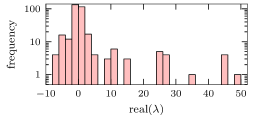
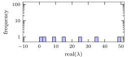
Figure 2: Eigenvalues and histograms of their distribution for the matrices $\widetilde{\textup{{M}}}$ (left) and M (right). The geometry is a unit semi-circle in 2D with homogeneous Dirichlet boundary conditions, E with bicubic interpolation ($p=3$), and a mesh spacing of $\Delta x=\frac{1}{32}$. Note the large number of eigenvalues near zero for $\widetilde{\textup{{M}}}$, whereas M correctly captures the spectrum of $1,4,9,16,25,\ldots$.

Remark

The computational band $L$ must be chosen so that it contains the interpolation stencil for $\textup{cp}(\boldsymbol{x})$ for all $\boldsymbol{x}$ needed in the calculation. Figure 3 shows the computational grid for an egg-shaped curve $\mathcal{S}$ illustrating the list of grid points $L$. An algorithm for the construction of the list $L$ is given in [20].

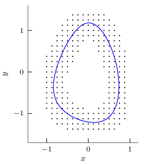
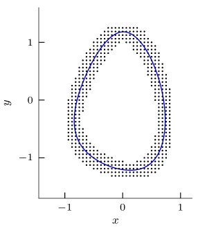
Figure 3: Computational grids for the Closest Point Method for an egg-shaped surface $\mathcal{S}$ with $\Delta x=0.125$ (left) and $\Delta x=0.0625$ (right). Second-order finite differences and degree $p=3$ interpolation.

4.4 Computing eigenvalues and eigenmodes

Given the discrete operator M which approximates the Laplace–Beltrami operator on a surface $\mathcal{S}$, we compute a spectral decomposition

$$\textup{{M}}=\textup{{Q}}\Lambda\textup{{Q}}^{-1},$$ (10)

where $\mathrm{diag}(\Lambda)$ are the eigenvalues of M and the columns of Q are the eigenvectors. These eigenvalues and eigenvectors are the respective approximations of the eigenvalues and eigenfunctions of the Laplace–Beltrami operator on $\mathcal{S}$.

4.4.1 Implementation

The final step of our algorithm—computing the spectral decomposition of a matrix M—is a well-known problem in numerical linear algebra (e.g., [22, 23]). For example, in Matlab we can use the function eig() to compute the complete decomposition or the function eigs() to compute only part of the spectrum. Matlab’s eig() calls LAPACK routines [24] and eigs() calls ARPACK [25] which makes use of the sparsity of the matrix M (in fact, it only requires a function which returns a matrix-vector product, although in this work we explicitly form the matrix M). Many of our calculations are performed in Python using SciPy [26] and NumPy [27] where we also make use of ARPACK via scipy.sparse.linalg.eigen.arpack.

The eigenfunctions are returned as vectors over the list of points $L$. In practice, the interpolation scheme from the closest point extension can be reused to evaluate the eigenfunctions at any desired points on the surface for plotting or other purposes.

4.4.2 Degree of interpolation

For the Closest Point Method to achieve the full order of accuracy of the underlying finite difference scheme (say $q$), the degree of interpolation $p$ must be chosen large enough so that the interpolant itself can be differentiated sufficiently accurately. For the second-order Laplace–Beltrami problems in this work, we need $p\geq q+1$ [17, 20].

5 Boundary conditions

When applied to an open surface, the Closest Point Method propagates boundary values into the embedding space along directions normal to the boundary, yielding homogeneous Neumann boundary conditions [17]. An analogous method for Dirichlet boundary conditions is similarly straightforward: instead of propagating out the interpolated values at boundary points the prescribed boundary conditions are propagated out [17]. While these methods are simple, they are only first-order accurate, which is lower-order than the discretizations of the Laplace–Beltrami operator discussed in this paper. Fortunately, a simple modification of the closest point function can be introduced to obtain a second-order accurate discretization for boundary conditions of Neumann or Dirichlet type.

Assume a smooth surface, and consider the following modification of the closest point function,

$$\bar{\textup{cp}}(\boldsymbol{x}):=\textup{cp}\big{(}\boldsymbol{x}+2(\textup{cp}(\boldsymbol{x})-\boldsymbol{x})\big{)}=\textup{cp}\big{(}2\textup{cp}(\boldsymbol{x})-\boldsymbol{x}\big{)}.$$ (11)

As is illustrated in Figure 4, whenever $\textup{cp}(\boldsymbol{x})$ is a point in the interior of the surface, the line between $2\textup{cp}(\boldsymbol{x})-\boldsymbol{x}$ and $\textup{cp}(\boldsymbol{x})$ is orthogonal to the surface. This implies that $\bar{\textup{cp}}(\boldsymbol{x})=\textup{cp}(2\textup{cp}(\boldsymbol{x})-\boldsymbol{x})=\textup{cp}(\boldsymbol{x})$, at least in a neighborhood of the surface. Conversely, if $\bar{\textup{cp}}(\boldsymbol{x}_{g})\neq\textup{cp}(\boldsymbol{x}_{g})$ for a point $\boldsymbol{x}_{g}$ then $\bar{\textup{cp}}(\boldsymbol{x}_{g})$ is an interior point of the surface and $\textup{cp}(\boldsymbol{x}_{g})$ is a boundary point. For a straight line or a planar surface, $u(\bar{\textup{cp}}(\boldsymbol{x}_{g}))$ gives the mirror value for $\boldsymbol{x}_{g}$, while for a general, curved surface it gives an approximate mirror value. In correspondence to the terminology for codimension-zero regions with boundaries, we call a point $\boldsymbol{x}_{g}$ a ghost point if $\textup{cp}(\boldsymbol{x}_{g})\neq\bar{\textup{cp}}(\boldsymbol{x}_{g})$ (and note this terminology differs slightly from [20]).

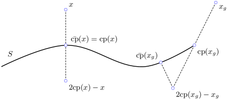
Figure 4: The function $\bar{\textup{cp}}$. For the point $\boldsymbol{x}$, the closest point $\textup{cp}(\boldsymbol{x})$ lies in the interior of the surface and for such a point, $\bar{\textup{cp}}(\boldsymbol{x})=\textup{cp}(\boldsymbol{x})$. However, for $\boldsymbol{x}_{g}$, the closest point $\textup{cp}(\boldsymbol{x}_{g})$ lies on the boundary of the surface and $\bar{\textup{cp}}(\boldsymbol{x}_{g})$ lies in the interior, with $\bar{\textup{cp}}(\boldsymbol{x}_{g})$ and $\boldsymbol{x}_{g}$ roughly equidistant from $\textup{cp}(\boldsymbol{x}_{g})$.

Thus, replacing $\textup{cp}(\boldsymbol{x})$ by $\bar{\textup{cp}}(\boldsymbol{x})$ in the Closest Point Method does not change the treatment of interior points. At ghost points, however, (approximate) mirror values are used. This yields a second-order approximation of homogeneous Neumann conditions; no other modification of the method is required. Homogeneous Dirichlet boundary conditions are obtained by extending the function at ghost points by $-u(\bar{\textup{cp}}(\boldsymbol{x}_{g}))$. By analogy to second-order boundary conditions for codimension-zero regions, we observe that an approximation of non-homogeneous Dirichlet conditions is obtained by extending at ghost points by $u(\boldsymbol{x}_{g})=2u(\textup{cp}(\boldsymbol{x}_{g}))-u(\bar{\textup{cp}}(\boldsymbol{x}_{g}))$, where $u(\textup{cp}(\boldsymbol{x}_{g}))$ is a prescribed value on the boundary.

We emphasize that the previous discussion relates to boundaries of the surface and the treatment of boundary conditions imposed thereat, not to the boundary of the narrow band of points (e.g., in Figure 3) where no artificial boundary condition need be applied [17, 20].

6 Numerical Results

We present a series of numerical examples to demonstrate the effectiveness of our approach.

6.1 Numerical convergence studies

We consider the egg-shaped curve in Figure 3 with arclength $2\pi$ as a test case. The Laplace–Beltrami eigenfunctions and eigenvalues in this case are the same as those of $u^{\prime\prime}=\lambda u$, where $u$ is $2\pi$ periodic, namely $u=\cos\left(ns+\beta\right)$ and $\lambda=n^{2}$ for $n\in\mathbb{Z}\geq 0$ where $s$ represents arclength and $\beta$ is a phase shift. The closest point function for this curve was determined using a numerical optimization procedure based on Newton’s method.

Figure 5 shows convergence studies in $\Delta x$ for the first few eigenvalues on the egg-shaped domain. For second-order finite differences and degree-three interpolation we observe second-order convergence. That is, the Closest Point Method approximates the eigenvalues with error $O(\Delta x^{2})$. Note that the error increases (and this is true even if one measures relative error) for the larger eigenvalues, but still shows second-order convergence. Figure 5 also shows that using fourth-order finite differences and degree-five interpolation, we get fourth-order accurate approximation to the eigenvalues.

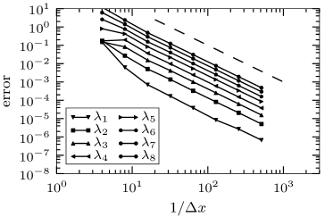
(a) 2nd-order FD, $p=3$ interp.

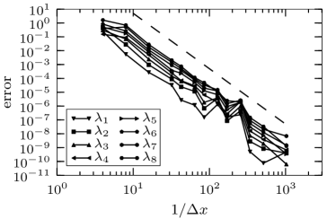
(b) 4th-order FD, $p=5$ interp.

Figure 5: Numerical convergence studies for eight of the Laplace–Beltrami eigenvalues ($\lambda_{n}=n^{2}$) of a closed egg-shaped curve in 2D. The dashed reference lines have slope two (left) and four (right). Note second-order accuracy using second-order finite differences with degree $p=3$ interpolation (left) and fourth-order accuracy using fourth-order finite differences with degree $p=5$ interpolation (right). The lack of smoothness in the fourth-order results plot may be because the underlying spline curve itself is only $C^{2}$ smooth; results on a circle (not included) are smoother.

In further numerical tests (not included), we found that degree $p=2$ interpolation with second-order finite differences, and degree $p=4$ interpolation with fourth-order finite differences, give approximately second- and fourth-order convergence, respectively. These are better than expected by one order of accuracy, as originally observed in [20].

6.1.1 Boundary Conditions

In this section we verify using convergence studies that our treatment of boundary conditions introduced in Section 5 achieves the expected order of accuracy. For our tests, we use the curve shown in Figure 6 parameterized as $(x(t),y(t))=(t,\cos t)$ for $t\in[1/4,4]$. We apply homogeneous Neumann and Dirichlet boundary conditions to the ends. Again, the exact eigenvalues and eigenfunctions can be determined analytically by considering the corresponding problem on an interval. For the former, the arclength of the curve is required and can be determined in terms of elliptic integrals.

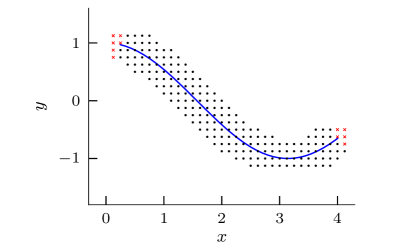
(a) 2nd-order FD, $p=3$ interp.

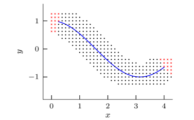
(b) 4th-order FD, $p=5$ interp.

Figure 6: A curve and the corresponding computational grids for the Closest Point Method with second-order (left) and fourth-order (right) finite difference schemes with $\Delta x=0.125$. Grid points marked with small crosses are the ghost points involved in implementing boundary conditions.

The original Closest Point Method, which does not explicitly treat boundaries, gives a first-order approximation to homogeneous boundary conditions [17]. See, for example, Figure 7 where it is observed that this trivial treatment of the boundaries limits the overall accuracy in the eigenvalues to first-order. Figure 7 also gives results using the new “$\bar{\textup{cp}}$” approach for Neumann boundary conditions described in Section 5; we find that this method attains the second-order accuracy of the underlying Cartesian finite difference scheme. Note that the $\bar{\textup{cp}}$ approach is also effective for Dirichlet boundary conditions. For example, in Figure 8 we find second-order results for homogeneous Dirichlet boundary conditions using $-u(\bar{\textup{cp}}(\boldsymbol{x}_{g})$ for ghost points (as in Section 5).

The $\bar{\textup{cp}}$ approach is designed to give second-order approximations to boundary conditions. Thus it is expected, and observed in Figure 8, that even with higher-order finite difference schemes and high-degree interpolation, the results will generally be second-order accurate in the presence of boundary conditions. Third- and higher-order approximation of boundary conditions may also be contemplated; while we do not investigate such methods here we note that approximations of this type will require a replacement for $\bar{\textup{cp}}$ that incorporates the curvature of the surface near the boundary.

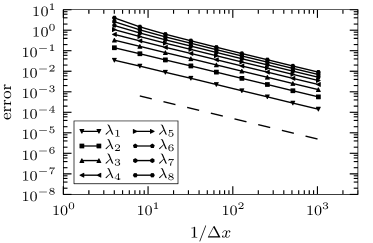
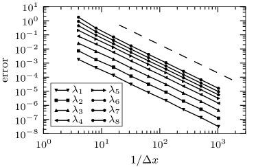
Figure 7: Numerical convergence studies for the first eight non-zero Laplace–Beltrami eigenvalues of a curve in 2D with Neumann boundary conditions applied at both ends. The left figure uses the original closest point function to impose a homogeneous Neumann boundary condition, and we note the results are only first-order accuracy (dashed reference line has slope one). The right figure uses the modified “$\bar{\textup{cp}}$” approach and exhibits second-order accuracy (dashed reference line has slope two). Both computations use second-order finite differences and degree $p=3$ interpolation.

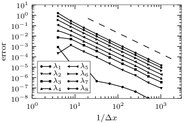
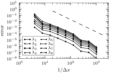
Figure 8: Numerical convergence study for the first few eigenvalues on a curve with Dirichlet boundary conditions applied at both ends. The boundaries are dealt with using the “$\bar{\textup{cp}}$” and $-u$ discretization with degree $p$ interpolation. The left figure uses second-order finite differences (and degree $p=3$ interpolation) and achieves second-order accuracy (the dashed reference lines have slope two). The right figure uses fourth-order finite differences (and degree $p=5$ interpolation) but the overall accuracy is limited by the second-order treatment of the boundary conditions.

6.1.2 Conditioning

Table 1 shows that the condition number of the matrices used in our computations scales like $O(\frac{1}{\Delta x^{2}})$. Thus the conditioning is the same as for standard Cartesian finite difference schemes. The “$\bar{\textup{cp}}$” treatment of boundary conditions does not have a significant effect on conditioning.

Table 1: Condition numbers (2-norm) for the matrix M. Tested for the Laplace–Beltrami operator on a open curve embedded in 2D with Dirichlet boundary conditions at both ends, using second-order finite differences, degree $p=3$ interpolation, and the “$\bar{\textup{cp}}$” treatment of the boundary conditions.

$\Delta x$	size of M	$\kappa(\textup{{M}})$
0.25	76 $\times$ 76	289
0.125	140 $\times$ 140	1154
0.0625	268 $\times$ 268	4608
0.03125	524 $\times$ 524	19304
0.015625	1036 $\times$ 1036	75543
0.0078125	2060 $\times$ 2060	326633

6.1.3 Behavior for high-frequency modes

The large number of spurious eigenvalues near $\frac{2d}{\Delta x^{2}}$ in Figure 9 reflect the singular behavior of Equation (8) at $\lambda=\frac{2d}{\Delta x^{2}}$ (c.f., Figure 2 where the problem instead occurs near the origin). Notably, it is these spurious eigenvalues which possess nonzero imaginary components, reflecting the fact that the eigenvalue problem (7) is not self-adjoint. Because these spurious eigenvalues correspond to highly oscillatory eigenfunctions which are quite close to the Nyquist frequency (i.e., with eigenvalues near $\frac{\pi^{2}}{\Delta x^{2}}$), it is not surprising that numerical difficulties arise for such modes. Nonetheless, any particular higher-frequency modes may be resolved by appropriately refining $\Delta x$.

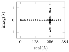
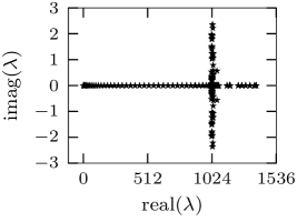
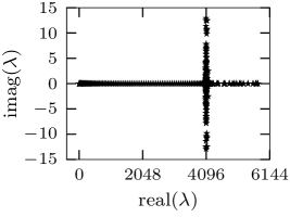
Figure 9: Computed spectra of the Laplace–Beltrami operator on a unit circle using $\Delta x=\frac{1}{8},\frac{1}{16}$, and $\frac{1}{32}$ (from left-to-right). The method uses second-order finite differences and degree $p=3$ interpolation. Note a large number of extraneous complex eigenvalues near $\frac{4}{\Delta x^{2}}$ (i.e., 256, 1024, and 4096): these correspond to the singularity in (8) and can be controlled by further resolving $\Delta x$.

6.2 Eigenfunction computations

The following computations were performed in Matlab and SciPy [26]. Visualizations were carried out with Matlab, VTK [28] and MayaVi [29].

6.2.1 Hemispherical harmonics

Figure 10 shows several Laplace–Beltrami eigenmodes of a unit hemisphere with homogeneous Neumann boundary conditions on the equator.

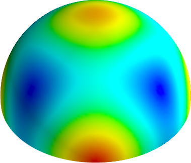
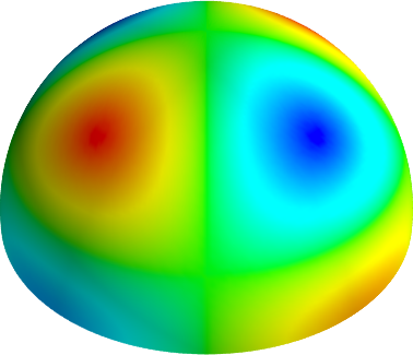
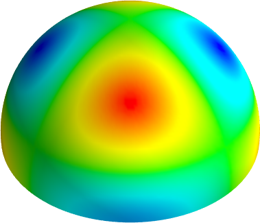
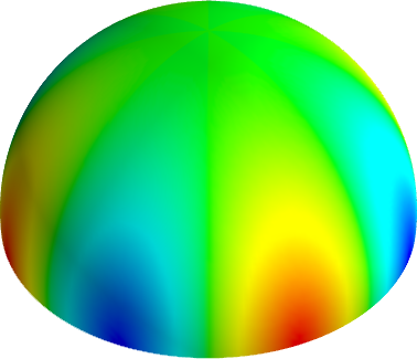
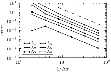
Figure 10: The left image shows several hemispherical harmonics with eigenvalue 20 computed with second-order finite differences, degree $p=3$ interpolation, and $\Delta x=\frac{1}{64}$. The right image is a convergence study for the first six eigenvalues ($\lambda_{n}=n(n+1)$), also using second-order finite differences and degree $p=3$ interpolation (the dashed reference line has slope two).

6.2.2 Eigenkaninchen

Figure 11 shows Laplace–Beltrami eigenmodes of the surface of the Stanford Bunny [30]. The closest point function for this and other triangulated surfaces can be computed in an efficient, straightforward manner [18].

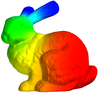
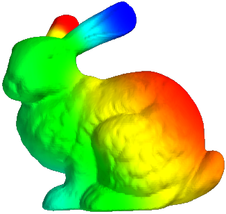
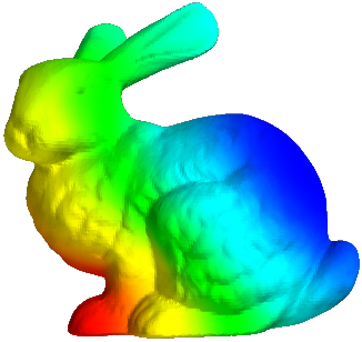
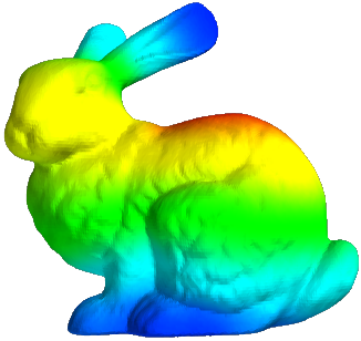
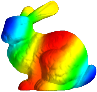
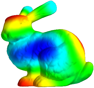
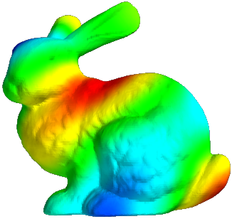
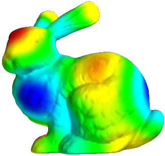
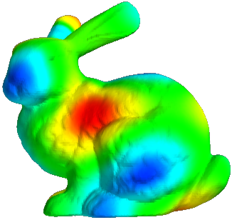
Figure 11: A selection of eigenkaninchen: Laplace–Beltrami eigenmodes on the surface of the Stanford Bunny [30]. The results are computed via the Closest Point Method using second-order finite differences, degree $p=3$ interpolation, and $\Delta x=0.1$, where the bunny is roughly two units long.

6.2.3 Möbius strip

Figure 12 shows some Laplace–Beltrami eigenmodes of a Möbius strip. Dirichlet boundary conditions are applied at the boundary of the Möbius strip. The surface is embedded in $\mathbb{R}^{3}$ and the closest point function for each grid point is computed from a parameterization using a numerical optimization procedure minimizing the square of the distance function. Note that the non-orientable nature of the Möbius strip poses no difficultly for the Closest Point Method.

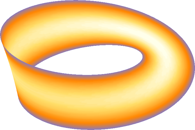
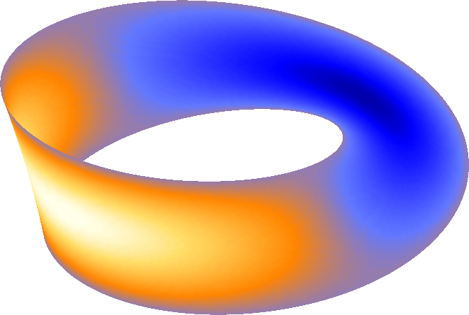
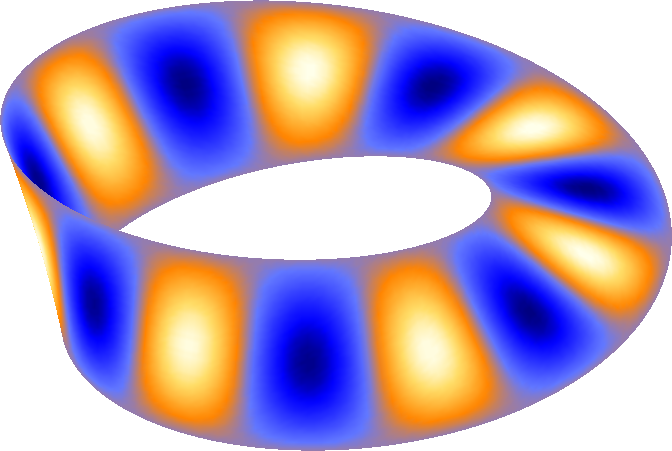
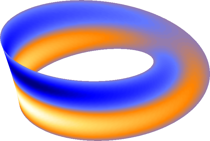
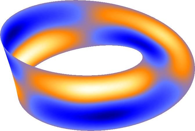
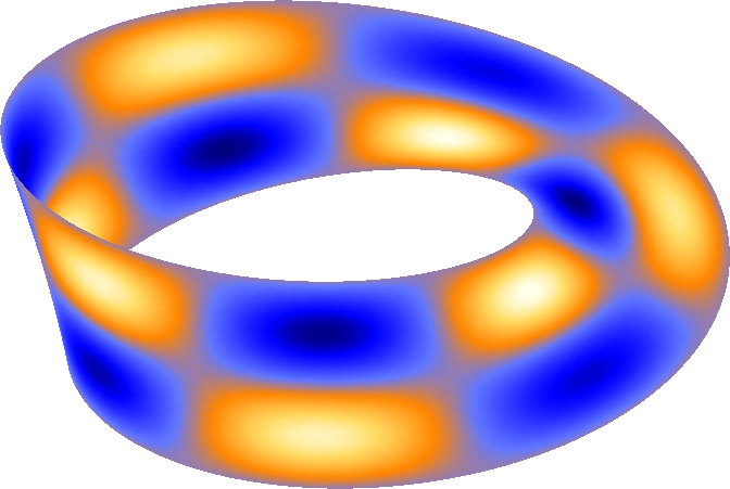
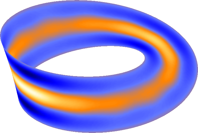
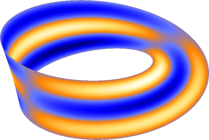
Figure 12: A selection of Laplace–Beltrami eigenmodes of a Möbius strip computed with the Closest Point Method. Calculations use second-order finite differences, $p=3$, $\Delta x=0.1$, and the Möbius strip is about 2 units in “diameter”.

6.2.4 L-shaped Domain

The Closest Point Method works on surfaces of various codimension [17, 20] and indeed solid shapes in $\mathbb{R}^{2}$ or $\mathbb{R}^{3}$ are surfaces of codimension-zero. Figure 13 shows an eigenmode computation on an L-shaped domain, where zero Dirichlet boundary conditions are imposed using the “$\bar{\textup{cp}}$” technique described in Section 5. In the interior of a solid, $\textup{cp}(\boldsymbol{x})=\boldsymbol{x}$ and so no interpolations are needed. Furthermore, for a grid-aligned L-shaped domain, for any $\boldsymbol{x}_{i}$ outside the domain, $\bar{\textup{cp}}(\boldsymbol{x}_{i})$ turns out to be another grid point $\boldsymbol{x}_{j}$ (located inside the domain as if the perimeter were a mirror) so no interpolation step is necessary. Thus in this special “corner case”, the Closest Point Method reduces to a standard finite difference computation using ghost points to mirror the values along the perimeter. Interestingly, these reductions happen automatically: no change in the code is needed.

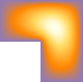
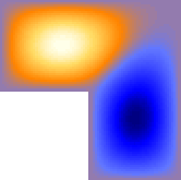
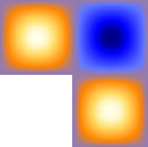
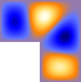
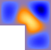
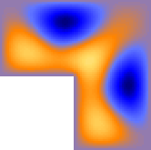
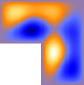
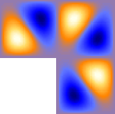
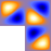
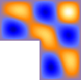
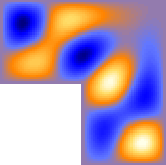
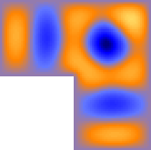
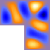
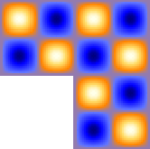
Figure 13: The first 15 Laplacian eigenmodes of an L-shaped domain with Dirichlet boundary conditions. The results are computed using the Closest Point Method with second-order finite differences using $\Delta x=1/40$ (the domain is two units wide).

6.2.5 Continental Africa

Some Laplace–Beltrami eigenmodes of continental Africa are shown in Figure 14. The results are computed directly on the surface of the Earth (assumed to be a sphere). Homogeneous Dirichlet boundary conditions are applied to the coastline. Finding the closest point function involves projecting onto a bitmapped image of the Earth [31] where the continent was first manually segmented. It is interesting to note that these eigenmodes match very closely the first ten eigenmodes of the L-shaped domain in Figure 13.

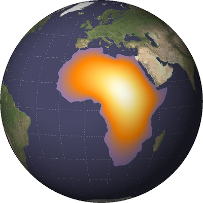
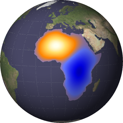
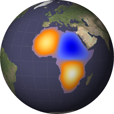
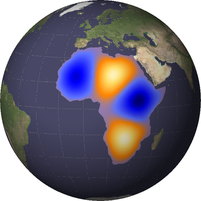
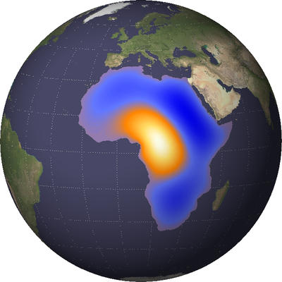
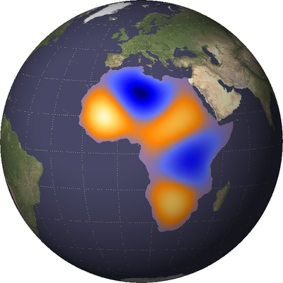
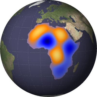
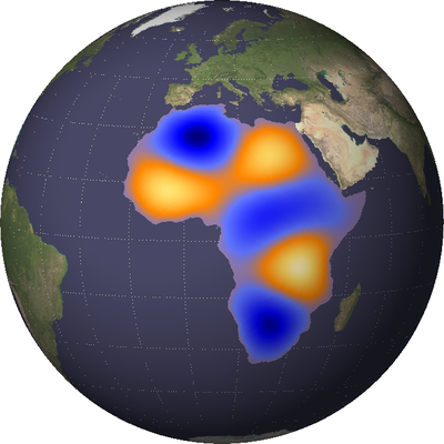
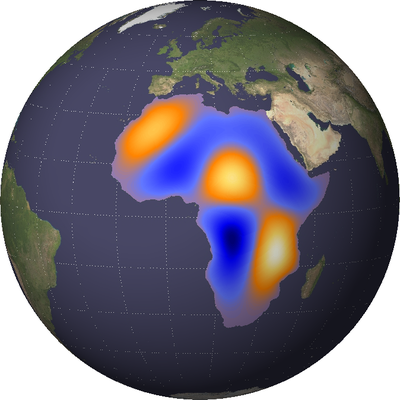
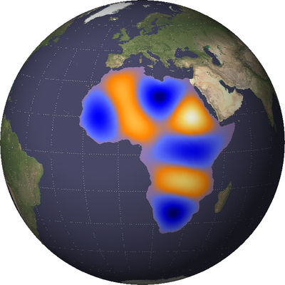
Figure 14: First ten eigenmodes of continental Africa. The Earth has unit diameter and the computation uses second-order finite differences with $\Delta x=1/40$ and degree $p=3$ interpolation.

7 Summary and Conclusions

Through a series of convergence studies and computational examples, we have shown that the Closest Point Method is an effective method for computing the spectra and eigenfunctions of the Laplace–Beltrami operator on rather general surfaces. The basis of our approach is the embedded eigenvalue problem (7) which, when discretized using standard, centered finite difference methods and Lagrange interpolation, yields a nonsymmetric matrix eigenvalue problem which can be solved using standard software. Fortunately, this lack of symmetry is not a concern in many practical situations since only the highest frequency modes have a significant imaginary component. We are currently investigating a finite element Closest Point Method which would lead to symmetric matrices.

For eigenvalue problems on open surfaces with Dirichlet or homogeneous Neumann boundary conditions, we have introduced second-order accurate schemes. These methods require only a simple change to the closest point extension and are straightforward to implement.

Although we have focused on the Laplace–Beltrami operator in this work, the Closest Point Method is applicable to many other surface differential operators [17, 18, 19, 20]. This suggests that the approach presented here may be applicable to a larger class of eigenvalue problems.

Finally, the techniques developed here are quite general and are applicable beyond surface eigenvalue problems. For example, future work will include solving surface Poisson problems of the form $-\Delta_{\mathcal{S}}u=f$.

Acknowledgments

The authors thank Bin Dong (UCSD), who motivated this work by asking if the Closest Point Method could be used for surface eigenvalue calculations.

Appendix A Additional theorems

As mentioned in Section 3.1, every solution to the ill-posed embedding problem (5), restricted to the surface, is a solution to the surface eigenvalue problem. Conversely, except for the $\lambda=0$ case, every surface eigenfunction corresponds to a unique solution of the embedding problem. These results are established by the following theorems.

Theorem 3

Suppose $v(\boldsymbol{x})$ and $\lambda$ are a solution to the embedding eigenvalue problem (5) and $\mathcal{S}$ is a smooth surface. Then $u:\mathcal{S}\to\mathbb{R}$ defined by $u(\boldsymbol{x})=v(\boldsymbol{x})$ for $\boldsymbol{x}\in\mathcal{S}$ is an eigenfunction of (4) with eigenvalue $\lambda$.

Proof 2

This is a direct consequence of Theorem 1.

Theorem 4

Let $\mathcal{S}$ be a smooth surface. For every non-constant solution $u$ and $\lambda$ of (4), there exists a unique (up to a multiplicative constant) eigenfunction $v$ of (5) with eigenvalue $\lambda$ which agrees with $u$ on $\mathcal{S}$. This eigenfunction is given by $v(\boldsymbol{x})=-\frac{1}{\lambda}\Delta(u(\textup{cp}(\boldsymbol{x}))).$

Proof 3

Using our hypothesis that $v$ agrees with $u$ on $\mathcal{S}$, we may solve for $v$ in (5) to obtain the result.

References

- [1] M. Reuter, F.-E. Wolter, N. Peinecke, Laplace-spectra as fingerprints for shape matching, in: Proceedings of the 2005 ACM symposium on Solid and physical modeling, SPM ’05, 2005, pp. 101–106. doi:10.1145/1060244.1060256.
- [2] M. Belkin, P. Niyogi, Laplacian eigenmaps for dimensionality reduction and data representation, Neural Computation 15 (6) (2003) 1373–1396. doi:10.1162/089976603321780317.
- [3] R. R. Coifman, S. Lafon, Diffusion maps, Applied and Computational Harmonic Analysis 21 (1) (2006) 5–30. doi:10.1016/j.acha.2006.04.006.
- [4] S. Seo, M. Chung, H. Vorperian, Heat kernel smoothing using Laplace–Beltrami eigenfunctions, in: T. Jiang, N. Navab, J. Pluim, M. Viergever (Eds.), Medical Image Computing and Computer-Assisted Intervention - MICCAI 2010, Vol. 6363 of Lecture Notes in Computer Science, Springer Berlin / Heidelberg, 2010, pp. 505–512. doi:10.1007/978-3-642-15711-0_63.
- [5] M. Reuter, S. Biasotti, D. Giorgi, G. Patanè, M. Spagnuolo, Discrete Laplace–Beltrami operators for shape analysis and segmentation, Computers & Graphics 33 (3) (2009) 381–390, iEEE International Conference on Shape Modelling and Applications 2009. doi:10.1016/j.cag.2009.03.005.
- [6] R. Glowinski, D. C. Sorensen, Computing the eigenvalues of the Laplace–Beltrami operator on the surface of a torus: A numerical approach, in: E. Oñate, R. Glowinski, P. Neittaanmäki (Eds.), Partial Differential Equations, Vol. 16 of Computational Methods in Applied Sciences, Springer Netherlands, 2008, pp. 225–232. doi:10.1007/978-1-4020-8758-5_12.
- [7] M. Reuter, F.-E. Wolter, N. Peinecke, Laplace–Beltrami spectra as ‘Shape-DNA’ of surfaces and solids, Computer-Aided Design 38 (4) (2006) 342–366. doi:10.1016/j.cad.2005.10.011.
- [8] J. Brandman, A level-set method for computing the eigenvalues of elliptic operators defined on compact hypersurfaces, J. Sci. Comput. 37 (2008) 282–315. doi:10.1007/s10915-008-9210-z.
- [9] M. Bertalmío, L.-T. Cheng, S. Osher, G. Sapiro, Variational problems and partial differential equations on implicit surfaces, J. Comput. Phys. 174 (2) (2001) 759–780.
- [10] J. Xu, H. Zhao, An Eulerian formulation for solving partial differential equations along a moving interface, J. Sci. Comput. 19 (1) (2003) 573–594. doi:10.1023/A:1025336916176.
- [11] J. B. Greer, A. L. Bertozzi, G. Sapiro, Fourth order partial differential equations on general geometries, J. Comput. Phys. 216 (1) (2006) 216–246.
- [12] J. B. Greer, An improvement of a recent Eulerian method for solving PDEs on general geometries, J. Sci. Comput. 29 (3) (2006) 321–352.
- [13] O. Nemitz, M. B. Nielsen, M. Rumpf, R. Whitaker, Finite element methods on very large, dynamic tubular grid encoded implicit surfaces, SIAM J. Sci. Comput.
- [14] G. Dziuk, C. M. Elliott, Eulerian finite element method for parabolic PDEs on implicit surfaces, Interf. Free Bound. 10 (2008) 119–138.
- [15] S. Leung, J. Lowengrub, H. Zhao, A grid based particle method for solving partial differential equations on evolving surfaces and modeling high order geometrical motion, J. Comput. Phys. 230 (7) (2011) 2540–2561. doi:10.1016/j.jcp.2010.12.029.
- [16] M. Floater, K. Hormann, Surface parameterization: a tutorial and survey, in: Advances in Multiresolution for Geometric Modelling, Springer, 2005, pp. 157–186.
- [17] S. J. Ruuth, B. Merriman, A simple embedding method for solving partial differential equations on surfaces, J. Comput. Phys. 227 (3) (2008) 1943–1961. doi:10.1016/j.jcp.2007.10.009.
- [18] C. B. Macdonald, S. J. Ruuth, Level set equations on surfaces via the Closest Point Method, J. Sci. Comput. 35 (2–3) (2008) 219–240. doi:10.1007/s10915-008-9196-6.
- [19] C. B. Macdonald, The Closest Point Method for time-dependent processes on surfaces, Ph.D. thesis, Simon Fraser University (August 2008).
- [20] C. B. Macdonald, S. J. Ruuth, The implicit Closest Point Method for the numerical solution of partial differential equations on surfaces, SIAM J. Sci. Comput. 31 (6) (2009) 4330–4350. doi:10.1137/080740003.
- [21] J.-P. Berrut, L. N. Trefethen, Barycentric Lagrange interpolation, SIAM Rev. 46 (3) (2004) 501–517.
- [22] G. H. Golub, C. F. van Loan, Matrix Computations, Johns Hopkins University Press, 1996.
- [23] L. N. Trefethen, D. Bau, Numerical Linear Algebra, SIAM, 1997.
- [24] E. Anderson, Z. Bai, C. Bischof, S. Blackford, J. Demmel, J. Dongarra, J. Du Croz, A. Greenbaum, S. Hammarling, A. McKenney, D. Sorensen, LAPACK Users’ Guide, 3rd Edition, SIAM, 1999.
- [25] R. Lehoucq, D. Sorensen, C. Yang, ARPACK Users’ Guide: Solution of Large-Scale Eigenvalue Problems with Implicitly Restarted Arnoldi Methods, SIAM, 1998.
- [26] E. Jones, T. Oliphant, P. Peterson, et al., SciPy: Open source scientific tools for Python, http://www.scipy.org, accessed 2008-07-15 (2001).
- [27] T. E. Oliphant, Python for scientific computing, Computing in Science & Engineering 9 (3) (2007) 10–20.
- [28] W. Schroeder, K. Martin, B. Lorensen, The Visualization Toolkit: an object-oriented approach to 3D graphics, Prentice Hall, 1998.
- [29] P. Ramachandran, G. Varoquaux, Mayavi: Making 3D data visualization reusable, in: G. Varoquaux, T. Vaught, J. Millman (Eds.), Proceedings of the 7th Python in Science Conference, 2008, pp. 51–56, http://code.enthought.com/projects/mayavi/.
- [30] G. Turk, M. Levoy, The Stanford Bunny, the Stanford 3D scanning repository, http://www-graphics.stanford.edu/data/3Dscanrep, accessed 2008-06-18 (1994).
- [31] NASA, Visible Earth website, http://visibleearth.nasa.gov, accessed 2010-12-05 (2010).