Tight conditions for consistency of variable selection in the context of high dimensionality

Abstract

We address the issue of variable selection in the regression model with very high ambient dimension, that is, when the number of variables is very large. The main focus is on the situation where the number of relevant variables, called intrinsic dimension, is much smaller than the ambient dimension $d$. Without assuming any parametric form of the underlying regression function, we get tight conditions making it possible to consistently estimate the set of relevant variables. These conditions relate the intrinsic dimension to the ambient dimension and to the sample size. The procedure that is provably consistent under these tight conditions is based on comparing quadratic functionals of the empirical Fourier coefficients with appropriately chosen threshold values.

The asymptotic analysis reveals the presence of two quite different re gimes. The first regime is when the intrinsic dimension is fixed. In this case the situation in nonparametric regression is the same as in linear regression, that is, consistent variable selection is possible if and only if $\log d$ is small compared to the sample size $n$. The picture is different in the second regime, that is, when the number of relevant variables denoted by $s$ tends to infinity as $n\to\infty$. Then we prove that consistent variable selection in nonparametric set-up is possible only if $s+\log\log d$ is small compared to $\log n$. We apply these results to derive minimax separation rates for the problem of variable selection.

T1Supported by the French Agence Nationale de la Recherche (ANR) under the grant PARCIMONIE.

and

1 Introduction

Real-world data such as those obtained from neuroscience, chemometrics, data mining or sensor-rich environments are often extremely high-dimensional, severely underconstrained (few data samples compared to the dimensionality of the data) and interspersed with a large number of irrelevant or redundant features. Furthermore, in most situations the data is contaminated by noise, making it even more difficult to retrieve useful information from the data. Relevant variable selection is a compelling approach for addressing statistical issues in the scenario of high-dimensional and noisy data with small sample size. Starting from Mallows Mallows , Akaike Akaike , Schwarz Schwarz who introduced, respectively, the famous criteria $C_{p}$, AIC and BIC, the problem of variable selection was extensively studied in the statistical and machine learning literature both from the theoretical and algorithmic viewpoints. It appears, however, that the theoretical limits of performing variable selection in the context of nonparametric regression are still poorly understood, especially when the number of variables, denoted by $d$ and referred to as ambient dimension, is much larger than the sample size $n$. The purpose of the present work is to explore this setting under the assumption that the number of relevant variables, hereafter called intrinsic dimension and denoted by $d^{*}$, may grow with the sample size but remains much smaller than $d$.

In the important particular case of linear regression, the latter scenario was the subject of a number of recent studies. Many of them rely on $\ell_{1}$-norm penalization Tibsh , Zhao , Meinshausen and constitute an attractive alternative to iterative variable selection procedures alquier , Zhang09 and to marginal regression or correlation screening Wass09 , Fan09 . Promising results for feature selection are also obtained by conformal prediction Hebiri2010 , (minimax) concave penalties Fan01 , Fan11 , ZhangCH10 , Bayesian approach Scott10 and higher criticism Donoho09 . Extensions to other settings including logistic regression, generalized linear model and Ising model were carried out in Bunea09 , Ravik , Fan09 , respectively. Variable selection in the context of groups of variables with disjoint or overlapping groups was studied by Yuan06 , svssin , Pontil , Obozinski , Huang10 . Hierarchical procedures for selection of relevant variables were proposed by Bach09 , Bickeletal , BinYu09 .

It is now well understood that in the Gaussian sequence model and in the high-dimensional linear regression with a Gram matrix satisfying some variant of irrepresentable condition, consistent estimation of the pattern of relevant variables—also called the sparsity pattern—is possible under the condition $d^{*}\log(d/d^{*})=o(n)$ as $n\to\infty$ Wainwright09 . Furthermore, it is well known that if $(d^{*}\log(d/d^{*}))/n$ remains bounded from below by some positive constant when $n\to\infty$, then it is impossible to consistently recover the sparsity pattern Verzelen10 . Thus, a tight condition exists that describes in an exhaustive manner the interplay between the quantities $d^{*}$, $d$ and $n$ that guarantees the existence of consistent estimators. The situation is very different in the case of nonlinear regression, since, to our knowledge, there is no result providing tight conditions for consistent estimation of the sparsity pattern.

Lafferty and Wasserman LaffertyWasserman and Bertin and Lecué BertinLecue , in papers closely related to the present work, considered the problem of variable selection in nonparametric Gaussian regression model. They proved the consistency of the proposed procedures under some assumptions that—in the light of the present work—turn out to be suboptimal. More precisely, Lafferty and Wasserman LaffertyWasserman assumed the unknown regression function to be four times continuously differentiable with bounded derivatives. The algorithm they proposed, termed Rodeo, is a greedy procedure performing simultaneously local bandwidth choice and variable selection. Rodeo is shown to converge when the ambient dimension $d$ is $O({\log n}/{\log\log n})$ while the intrinsic dimension $d^{*}$ does not increase with $n$. On the other hand, Bertin and Lecué BertinLecue proposed a procedure based on the $\ell_{1}$-penalization of local polynomial estimators and proved its consistency when $d^{*}=O(1)$, but $d$ is allowed to be as large as $\log n$, up to a constant. They also had a weaker assumption on the regression function merely assumed to belong to the Holder class with smoothness $\beta>1$. To complete the picture, let us mention that estimation and hypotheses testing problems for high-dimensional nonparametric regression under sparse additive modeling were recently addressed in Koltchinskii10 , Raskuttietal , GayraudIngster .

This brief review of the literature reveals that there is an important gap in consistency conditions for the linear regression and for the nonlinear one. For instance, if the intrinsic dimension $d^{*}$ is fixed, then the condition guaranteeing consistent estimation of the sparsity pattern is $(\log d)/n\to 0$ in linear regression, whereas it is $d=O(\log n)$ in the nonparametric case. While it is undeniable that the nonparametric regression is much more complex than the linear one, it is, however, not easy to find a justification to such an important gap between two conditions. The situation is even worse in the case where $d^{*}\to\infty$. In fact, for the linear model with at most polynomially increasing ambient dimension $d=O(n^{k})$, it is possible to estimate the sparsity pattern for intrinsic dimensions $d^{*}$ as large as $n^{1-\varepsilon}$, for some $\varepsilon>0$. In other words, the sparsity index can be almost on the same order as the sample size. In contrast, in nonparametric regression, there is no procedure that is proved to converge to the true sparsity pattern when both $n$ and $d^{*}$ tend to infinity, even if $d^{*}$ grows extremely slowly.

In the present work, we fill this gap by introducing a simple variable selection procedure that selects the relevant variables by comparing some quadratic functionals of empirical Fourier coefficients to prescribed significance levels. Consistency of this procedure is established under some conditions on the triplet $(d^{*},d,n)$, and the tightness of these conditions is proved. The main take-away messages deduced from our results are the following:

• When the number of relevant variables $d^{*}$ is fixed and the sample size $n$ tends to infinity, there exist positive real numbers ${c}_{*}$ and ${c}^{*}$ such that (a) if $(\log d)/n\leq{c}_{*}$ the estimator proposed in Section 3 is consistent and (b) no estimator of the sparsity pattern may be consistent if $(\log d)/n\geq{c}^{*}$.

• When the number of relevant variables $d^{*}$ tends to infinity with $n\to\infty$, then there exist real numbers $\underline{c}_{i}$ and $\bar{c}_{i}$, $i=1,2$ such that $\underline{c}_{1}>0$, $\bar{c}_{1}>0$ and (a) if $\underline{c}_{1}d^{*}+\log\log(d/d^{*})-\log n<\underline{c}_{2}$ the estimator proposed in Section 3 is consistent and (b) no estimator of the sparsity pattern may be consistent if $\bar{c}_{1}d^{*}+\log\log(d/d^{*})-\log n>\bar{c}_{2}$.

• In particular, if $d$ grows not faster than a polynomial in $n$, then there exist positive real numbers ${c}_{0}$ and ${c}^{0}$ such that (a) if $d^{*}\leq{c}_{0}\log n$, the estimator proposed in Section 3 is consistent, and (b) no estimator of the sparsity pattern may be consistent if $d^{*}\geq{c}^{0}\log n$.

In the regime of a growing intrinsic dimension $d^{*}\to\infty$ and a moderately large ambient dimension $d=O(n^{C})$, for some $C>0$, we make a concentrated effort to get the constant $c_{0}$ as close as possible to the constant $c^{0}$. This goal is reached for the model of Gaussian white noise and, very surprisingly, it required from us to apply some tools from complex analysis, such as the Jacobi $\theta$-function and the saddle point method, in order to evaluate the number of lattice points lying in a ball of an Euclidean space with increasing dimension.

The rest of the paper is organized as follows. The notation and assumptions necessary for stating our main results are presented in Section 2. In Section 3, an estimator of the set of relevant variables is introduced and its consistency is established, in the case where the data come from the Gaussian white noise model. The main condition required in the consistency result involves the number of lattice points in a ball of a high-dimensional Euclidean space. An asymptotic equivalent for this number is presented in Section 4. Results on impossibility of consistent estimation of the sparsity pattern are derived in Section 5. Section 6 is devoted to exploring adaptation to the unknown parameters (smoothness and degree of significance) and recovering minimax rates of separation. Then, in Section 7, we show that some of our results can be extended to the model of nonparametric regression. The relations between consistency and inconsistency results are discussed in Section 8. The technical parts of the proofs are postponed to the Appendix.

2 The problem formulation and the assumptions

We are interested in the variable selection task (also known as model selection, feature selection, sparsity pattern estimation) in the context of high-dimensional nonlinear regression. Let $\mathsf{f}\dvtx[0,1]^{d}\to\mathbb{R}$ denote the unknown regression function. We assume that the number of variables $d$ is very large, possibly much larger than the sample size $n$, but only a small number of these variables contribute to the fluctuations of the regression function $\mathsf{f}$.

To be more precise, we assume that for some small subset $J$ of the index set $\{1,\ldots,d\}$ satisfying $\operatorname{Card}(J)\leq d^{*}$, there is a function $\bar{\mathsf{f}}\dvtx\mathbb{R}^{\mathrm{Card}(J)}\to\mathbb{R}$ such that

$$\mathsf{f}(\mathbf{x})=\bar{\mathsf{f}}(\mathbf{x}_{J})\qquad\forall\mathbf{x}\in\mathbb{R}^{d},$$

where $\mathbf{x}_{J}$ stands for the subvector of $\mathbf{x}$ obtained by removing from $\mathbf{x}$ all the coordinates with indices lying outside $J$. In what follows, we allow $d$ and $d^{*}$ to depend on $n$, but we will not always indicate this dependence in notation. Note also that the genuine intrinsic dimension is $\operatorname{Card}(J)$; $d^{*}$ is merely a known upper bound on the intrinsic dimension. In what follows, we use the standard notation for the vector and sequence norms:

$$\|\mathbf{x}\|_{0} = \sum_{j}\mathbf{1}(x_{j}\not=0),\qquad\|\mathbf{x}\|_{p}^{p}=\sum_{j}|x_{j}|^{p}\qquad\forall p\in[1,\infty),$$

$$\|\mathbf{x}\|_{\infty} = \sup_{j}|x_{j}|$$

for every $\mathbf{x}\in\mathbb{R}^{d}$ or $\mathbf{x}\in\mathbb{R}^{\mathbb{N}}$.

Let us stress right away that the primary aim of this work is to understand when it is possible to estimate the sparsity pattern $J$ (with theoretical guarantees on the convergence of the estimator) and when it is impossible. The estimator that we will define in the next sections is intended to show the possibility of consistent estimation, rather than to provide a practical procedure for recovering the sparsity pattern. Therefore, the estimator will be allowed to depend on different constants appearing in conditions imposed on the regression function $\mathsf{f}$ and on some characteristics of the noise.

To make the consistent estimation of the set $J$ realizable, we impose some smoothness and identifiability assumptions on $\mathsf{f}$. In order to describe the smoothness assumption imposed on $\mathsf{f}$, let us introduce the trigonometric Fourier basis, $\varphi_{\mathbf{0}}\equiv 1$ and

$$\varphi_{\mathbf{k}}(\mathbf{x})=\cases{\sqrt{2}\cos(2\pi\mathbf{k}\cdot\mathbf{x}),&\quad$\mathbf{k}\in\bigl{(}\mathbb{Z}^{d}\bigr{)}_{+},$\vspace*{2pt}\cr\sqrt{2}\sin(2\pi\mathbf{k}\cdot\mathbf{x}),&\quad$-\mathbf{k}\in\bigl{(}\mathbb{Z}^{d}\bigr{)}_{+},$}$$ (1)

where $(\mathbb{Z}^{d})_{+}$ denotes the set of all $\mathbf{k}\in\mathbb{Z}^{d}\setminus\{0\}$ such that the first nonzero element of $\mathbf{k}$ is positive, and $\mathbf{k}\cdot\mathbf{x}$ stands for the usual inner product in $\mathbb{R}^{d}$. In what follows, we use the notation $\langle\cdot,\cdot\rangle$ for designing the scalar product in $L^{2}([0,1]^{d};\mathbb{R})$, that is, $\langle\mathsf{h},\tilde{\mathsf{h}}\rangle=\int_{[0,1]^{d}}\mathsf{h}(\mathbf{x})\tilde{\mathsf{h}}(\mathbf{x})\,d\mathbf{x}$ for every $\mathsf{h},\tilde{\mathsf{h}}\in L^{2}([0,1]^{d};\mathbb{R})$. Using this orthonormal Fourier basis, we define

$$\Sigma_{L}=\biggl{\{}f\dvtx\sum_{\mathbf{k}\in\mathbb{Z}^{d}}k_{j}^{2}\langle\mathsf{f},\varphi_{\mathbf{k}}\rangle^{2}\leq L;\forall j\in\{1,\ldots,d\}\biggr{\}}.$$

To ease notation, we set $\theta_{\mathbf{k}}[\mathsf{f}]=\langle\mathsf{f},\varphi_{\mathbf{k}}\rangle$ for all $\mathbf{k}\in\mathbb{Z}^{d}$. In addition to the smoothness, we need also to require that the relevant variables are sufficiently relevant for making their identification possible. This is done by means of the following condition. [[C1$(\kappa,L)$]]

The regression function $\mathsf{f}$ belongs to $\Sigma_{L}$. Furthermore, for some subset $J\subset\{1,\ldots,d\}$ of cardinality $\leq d^{*}$, there exists a function $\bar{\mathsf{f}}\dvtx\mathbb{R}^{\mathrm{Card}(J)}\to\mathbb{R}$ such that $\mathsf{f}(\mathbf{x})=\bar{\mathsf{f}}(\mathbf{x}_{J})$, $\forall\mathbf{x}\in\mathbb{R}^{d}$, and it holds that

$$Q_{j}[\mathsf{f}]=\sum_{\mathbf{k}:k_{j}\neq 0}\theta_{\mathbf{k}}[\mathsf{f}]^{2}\geq\kappa\qquad\forall j\in J.$$ (2)

One easily checks that $Q_{j}[\mathsf{f}]=0$ for every $j$ that does not lie in the sparsity pattern. This provides a characterization of the sparsity pattern as the set of indices of nonzero coefficients of the vector $\mathbf{Q}[\mathsf{f}]=(Q_{1}[\mathsf{f}],\ldots,Q_{d}[\mathsf{f}])$.

Prior to describing the procedures for estimating $J$, let us comment on condition [C1]. It is important to note that the identifiability assumption (2) can be rewritten as $\int_{[0,1]^{d}}(\mathsf{f}(\mathbf{x})-\int_{0}^{1}\mathsf{f}(\mathbf{x})\,dx_{j})^{2}\,d\mathbf{x}\geq\kappa$ and, therefore, is not intrinsically related to the basis we have chosen. In the case of continuously differentiable and $1$-periodic function $\mathsf{f}$, the smoothness assumption $\mathsf{f}\in\Sigma_{L}$ as well can be rewritten without using the trigonometric basis, since $\sum_{\mathbf{k}\in\mathbb{Z}^{d}}k_{j}^{2}\theta_{\mathbf{k}}[\mathsf{f}]^{2}=(2\pi)^{-2}\int_{[0,1]^{d}}[\partial_{j}\mathsf{f}(\mathbf{x})]^{2}\,d\mathbf{x}$. Thus condition [C1] is essentially a constraint on the function $\mathsf{f}$ itself and not on its representation in the specific basis of trigonometric functions.

The results of this work can be extended with minor modifications to other types of smoothness conditions imposed on $\mathsf{f}$, such as Hölder continuity or Besov-regularity. In these cases the trigonometric basis (1) should be replaced by a basis adapted to the smoothness condition (spline, wavelet, etc.). Furthermore, even in the case of Sobolev smoothness, one can replace the set $\Sigma_{L}$ corresponding to smoothness order $1$ by any Sobolev ellipsoid of smoothness $\beta>0$; see, for instance, LaetCRASS where the case $\beta=2$ is explored. Roughly speaking, the role of the smoothness assumption is to reduce the statistical model with infinite-dimensional parameter $\mathsf{f}$ to a finite-dimensional model having good approximation properties. Any value of smoothness order $\beta>0$ leads to this reduction. The value $\beta=1$ is chosen for simplicity of exposition only.

3 Idealized setup: Gaussian white noise model

To convey the main ideas without taking care of some technical details, we start by focusing our attention on the Gaussian white noise model that was proved to be asymptotically equivalent to the model of regression BrownLow96 , Reiss08 , as well as to other nonparametric models Brown04 , DalReiss06 . Thus, we assume that the available data consists of the Gaussian process $\{\mathbf{Y}(\phi)\dvtx\phi\in L^{2}([0,1]^{d};\mathbb{R})\}$ such that

$$\mathbb{E}_{\mathsf{f}}\bigl{[}\mathbf{Y}(\phi)\bigr{]}=\int_{[0,1]^{d}}\mathsf{f}(\mathbf{x})\phi(\mathbf{x})\,d\mathbf{x},\qquad\operatorname{Cov}_{f}\bigl{(}\mathbf{Y}(\phi),\mathbf{Y}\bigl{(}\phi^{\prime}\bigr{)}\bigr{)}=\frac{1}{n}\int_{[0,1]^{d}}\phi(\mathbf{x})\phi^{\prime}(\mathbf{x})\,d\mathbf{x}.$$

It is well known that these two properties uniquely characterize the probability distribution of a Gaussian process. An alternative representation of $\mathbf{Y}$ is

$$dY(\mathbf{x})=\mathsf{f}(\mathbf{x})\,d\mathbf{x}+n^{-1/2}\,dW(\mathbf{x}),\qquad\mathbf{x}\in[0,1]^{d},$$

where $W(\mathbf{x})$ is a $d$-parameter Brownian sheet. Note that minimax estimation and detection of the function $\mathsf{f}$ in this set-up (but without sparsity assumption) was studied by Ingster07 .

3.1 Estimation of $J$ by multiple hypotheses testing

We intend to tackle the variable selection problem by multiple hypotheses testing; each hypothesis concerns a group of the Fourier coefficients of the observed signal and suggests that all the elements within the group are zero. The rationale behind this approach is the following simple observation: since the trigonometric basis is orthonormal and contains the constant function,

$$j\notin J\quad\Longleftrightarrow\quad\theta_{\mathbf{k}}[\mathsf{f}]=\langle f,\varphi_{\mathbf{k}}\rangle=0\qquad\forall\mathbf{k}\mbox{ s.t. }k_{j}\not=0.$$ (3)

This observation entails that if the intrinsic dimension $|J|$ is small as compared to $d$, then the sequence of Fourier coefficients is sparse. Furthermore, as explained below, there is a sort of group sparsity with overlapping groups.

For every $\ell\in\{1,\ldots,d^{*}\}$, we denote by $P_{\ell}^{d}$ the set of all subsets $I$ of $\{1,\ldots,d\}$ having exactly $\ell$ elements: $P_{\ell}^{d}=\{I\subset\{1,\ldots,d\}\dvtx\operatorname{Card}(I)=\ell\}$. For every multi-index $\mathbf{k}\in\mathbb{Z}^{d}$, we denote by $\mathop{\operatorname{supp}}(\mathbf{k})$ the set of indices corresponding to nonzero entries of $\mathbf{k}$. To define the blocks of coefficients $\theta_{\mathbf{k}}$ that will be tested for significance, we introduce the following notation: for every $I\subset\{1,\ldots,d\}$ and for every $j\in I$, we set

$$V_{I}^{j}[\mathsf{f}]=\bigl{(}\theta_{\mathbf{k}}[\mathsf{f}]\dvtx j\in\mathop{\operatorname{supp}}(\mathbf{k})\subset I\bigr{)}.$$

It follows from (3) that the characterization

$$j\notin J\quad\Longleftrightarrow\quad\max_{I}\bigl{\|}V_{I}^{j}[\mathsf{f}]\bigr{\|}_{p}=0,$$ (4)

holds true for every $p\in[0,+\infty]$. Furthermore, again in view of (3), the maximum over $I$ of the norms $\|V_{I}^{j}[\mathsf{f}]\|_{p}$ is attained when $I=J$ and is equal to the maximum over all subsets $I$ such that $\operatorname{Card}(I)\leq d^{*}$. Summarizing these arguments, we can formulate the problem of variable selection as a problem of testing $d$ null hypotheses

$$H_{0j}\dvtx\bigl{\|}V_{I}^{j}[\mathsf{f}]\bigr{\|}_{p}=0\qquad\forall I\subset\{1,\ldots,d\}\mbox{ such that }\operatorname{Card}(I)\leq d^{*}.$$ (5)

If the hypothesis $H_{0j}$ is rejected, then the $j$th covariate is declared as relevant. Note that by virtue of assumption [C1], the alternatives can be written as

$$H_{1j}\dvtx\bigl{\|}V_{I}^{j}[\mathsf{f}]\bigr{\|}_{2}^{2}\geq\kappa\qquad\mbox{for some }I\subset\{1,\ldots,d\}\mbox{ such that }\operatorname{Card}(I)\leq d^{*}.$$ (6)

Our estimator is based on this characterization of the sparsity pattern. If we denote by $y_{\mathbf{k}}$ the observable random variable $\mathbf{Y}(\varphi_{\mathbf{k}})$, we have

$$y_{\mathbf{k}}=\theta_{\mathbf{k}}[\mathsf{f}]+n^{-1/2}\xi_{\mathbf{k}},\qquad\theta_{\mathbf{k}}=\langle f,\varphi_{\mathbf{k}}\rangle,\mathbf{k}\in\mathbb{Z}^{d},$$ (7)

where $\{\xi_{\mathbf{k}};\mathbf{k}\in\mathbb{Z}^{d}\}$ form a countable family of independent Gaussian random variables with zero mean and variance equal to one. According to this property, $y_{\mathbf{k}}$ is a good estimate of $\theta_{\mathbf{k}}[\mathsf{f}]$: it is unbiased and with a mean squared error equal to $1/n$. Using the plug-in argument, this suggests to estimate $V_{I}^{j}$ by $\widehat{V}_{I}^{j}=(y_{\mathbf{k}}\dvtx j\in\mathop{\operatorname{supp}}(\mathbf{k})\subset I)$ and the norm of $V_{I}^{j}$ by the norm of $\widehat{V}_{I}^{j}$. However, since this amounts to estimating an infinite-dimensional vector, the error of estimation will be infinitely large. To cope with this issue, we restrict the set of indices for which $\theta_{\mathbf{k}}$ is estimated by $y_{\mathbf{k}}$ to a finite set, outside of which $\theta_{\mathbf{k}}$ will be merely estimated by $0$. Such a restriction is justified by the fact that $\mathsf{f}$ is assumed to be smooth: Fourier coefficients corresponding to very high frequencies are very small.

Let us fix an integer $m>0$, the cut-off level, and denote, for $j\in I\subset\{1,\ldots,d\}$,

$$S^{j}_{m,I}=\bigl{\{}\mathbf{k}\in\mathbb{Z}^{d}\dvtx\|\mathbf{k}\|_{2}\leq m\mbox{ and }\{j\}\subset\operatorname{supp}(\mathbf{k})\subset I\bigr{\}}.$$

Since the alternatives $H_{1j}$ are concerned with the 2-norm, we build our test statistic on an estimate of the norm $\|V_{I}^{j}[\mathsf{f}]\|_{2}$. To this end, we introduce

$$\widehat{Q}_{m,I}^{j}=\sum_{\mathbf{k}\in S^{j}_{m,I}}\biggl{(}y_{\mathbf{k}}^{2}-\frac{1}{n}\biggr{)},$$

which is an unbiased estimator of $Q_{m,I}^{j}=\sum_{\mathbf{k}\in S^{j}_{m,I}}\theta_{\mathbf{k}}^{2}$. Note that when $m\to\infty$, the quantity $Q_{m,I}^{j}$ approaches $\|V_{I}^{j}[\mathsf{f}]\|_{2}^{2}$. It is clear that larger values of $m$ lead to a smaller bias while the variance get increased. Moreover, the variance of $\widehat{Q}_{m,I}^{j}$ is proportional to the cardinality of the set $S^{j}_{m,I}$. The latter is an increasing function of $\operatorname{Card}(I)$. Therefore, if we aim at getting comparable estimation accuracies when estimating the functionals $\|V_{I}^{j}[\mathsf{f}]\|_{2}^{2}$ by $\widehat{Q}_{m,I}^{j}$ for various $I$’s, it is reasonable to make the cut-off level $m$ vary with the cardinality of $I$.

Thus, we consider a multivariate cut-off $\mathbf{m}=(m_{1},\ldots,m_{d^{*}})\in\mathbb{N}^{d^{*}}$. For a subset $I$ of cardinality $\ell\leq d^{*}$, we test significance of the vector $V_{I}^{j}[\mathsf{f}]$ by comparing its estimate $\widehat{Q}_{m_{\ell},I}^{j}$ with a prescribed threshold $\lambda_{\ell}$. This leads us to define an estimator of the set $J$ by

$$\widehat{J}_{n}(\mathbf{m},\bolds{\lambda})=\Bigl{\{}j\in\{1,\ldots,d\}\dvtx\max_{\ell\leq d^{*}}\lambda_{\ell}^{-1}\max_{I\in P^{d}_{\ell}}\widehat{Q}_{m_{\ell},I}^{j}\geq 1\Bigr{\}},$$

where $\mathbf{m}=(m_{1},\ldots,m_{d^{*}})\in\mathbb{N}^{d^{*}}$ and $\bolds{\lambda}=(\lambda_{1},\ldots,\lambda_{d^{*}})\in\mathbb{R}^{d^{*}}_{+}$ are two vectors of tuning parameters. As already mentioned, the role of $\mathbf{m}$ is to ensure that the truncated sums $Q_{m,J}^{j}$ do not deviate too much from the complete sums $Q_{J}^{j}$. Quantitatively speaking, for a given $\tau>0$, we would like to choose $m_{\ell}$’s so that $Q_{m_{s},J}^{j}\geq\kappa\tau/\tau+1$, where $s=\operatorname{Card}(J)$. This guarantee can be achieved due to the smoothness assumption. Indeed, as proved in (B) (cf. Appendix B), it holds that

$$Q_{m_{s},J}^{j}\geq\kappa-m_{s}^{-2}Ls\qquad\forall j\in J.$$

Therefore, choosing $m_{\ell}=(\ell L(1+\tau)/\kappa)^{1/2}$, for every $\ell=1,\ldots,d^{*}$, entails the inequality $Q_{m_{s},J}^{j}\geq\kappa\tau/\tau+1$, which indicates that the relevance of variables is not affected too much by the truncation.

Pushing further the analogy with the hypotheses testing, we define type I error of an estimator $\widehat{J}_{n}$ of $J$ as the one of having $\widehat{J}_{n}\not\subset J$, that is, classifying some irrelevant variables as relevant. The type II error is then that of having $J\not\subset\widehat{J}$, which amounts to classifying some relevant variables as irrelevant. As in the testing problem, handling the type I error is easier since the distribution of the test statistic is independent of $\mathsf{f}$. In fact, this is the max of a finite family of random variables drawn from translated and scaled $\chi^{2}$-distributions. Using the Bonferroni adjustment leads to the following control of the first kind error.

Proposition 1

Let us denote by $N(\ell,\gamma)$ the cardinality of the set $\{\mathbf{k}\in\mathbb{Z}^{\ell}\dvtx\|\mathbf{k}\|_{2}^{2}\leq\gamma\ell\ \&\ k_{1}\not=0\}$. If for some $A>1$ and for every $\ell=1,\ldots,d^{*}$,

$$\lambda_{\ell}\geq\frac{2\sqrt{AN(\ell,m_{\ell}^{2}/\ell)d^{*}\log(2ed/d^{*})}+2Ad^{*}\log(2ed/d^{*})}{n},$$ (8)

then the type I error $\mathbf{P}(\widehat{J}_{n}(\mathbf{m},\bolds{\lambda})\not\subset J)$ is upper-bounded by $(2ed/d^{*})^{-d^{*}(A-1)}$, and therefore tends to 0 as $d\to+\infty$.

This proposition shows that the type I error of a variable selection procedure may be made small by choosing a sufficiently high threshold. By doing this, we run the risk to reject $H_{0j}$ very often and to drastically underestimate the set of relevant variables. The next result establishes a necessary condition, which will be shown to be tight, ensuring that such an underestimation does not occur.

Theorem 1

Let condition [C1$(\kappa,L)$] be satisfied with some known constants $\kappa>0$ and $L<\infty$, and let $s=\operatorname{Card}(J)$. For some real numbers $\tau>0$ and $A>1$, set $m_{\ell}=(\ell L(1+\tau)/\kappa)^{1/2}$, $\ell=1,\ldots,d^{*}$, and define $\lambda_{\ell}$ to be equal to the right-hand side of (8). If the condition

$$4\lambda_{s}\leq{\kappa\tau}/{(1+\tau)}$$ (9)

is fulfilled, then $\widehat{J}_{n}(\mathbf{m},\bolds{\lambda})$ is consistent and satisfies the inequalities $\mathbf{P}(\widehat{J}_{n}(\mathbf{m},\break\bolds{\lambda})\not\supset J)\leq 2(2ed/d^{*})^{-d^{*}(A-1)}$ and $\mathbf{P}(\widehat{J}_{n}(\mathbf{m},\bolds{\lambda})\not=J)\leq 3(2ed/d^{*})^{-d^{*}(A-1)}$.

Condition (9), ensuring the consistency of the variable selection procedure $\widehat{J}_{n}$, admits a very natural interpretation: It is possible to detect relevant variables if the degree of relevance $\kappa$ is larger than a multiple of the threshold $\lambda_{s}$, the latter being chosen according to the noise level.

A first observation is that this theorem provides interesting insight to the possibility of consistent recovery of the sparsity pattern $J$ in the context of fixed intrinsic dimension. In fact, when $d^{*}$ remains bounded from above when $n\!\to\!\infty$ and $d\!\to\!\infty$, then we get that $\mathbf{P}(\widehat{J}_{1}(m,\lambda)=J)\!\to\!_{n,d\to\infty}1$ provided that

$$\log d\leq\operatorname{Const}\cdot n.$$ (10)

Although we did not find (exactly) this result in the statistical literature on variable selection, it can be checked that (10) is a necessary and sufficient condition for recovering the sparsity pattern $J$ in linear regression with fixed sparsity $d^{*}$ and growing dimension $d$ and sample size $n$. Thus, in the regime of fixed or bounded $d^{*}$, the sparsity pattern estimation in nonparametric regression is not more difficult than in the parametric linear regression, as far as only the consistency of estimation is considered and the precise value of the constant in (10) is neglected. Furthermore, there is a simple estimator $\widehat{J}_{n}^{(1)}$ of $J$ (cf. equation (3) in LaetCRASS ), which is provably consistent under condition (10). This estimator can be seen as a procedure of testing hypotheses $H_{0j}$ of form (5) with $p=\infty$ and, therefore, it does not really exploit the structure of the Fourier coefficients of the regression function. To some extent, this is the reason why in the regime of growing intrinsic dimension $d^{*}\to\infty$, the estimator $\widehat{J}_{n}^{(1)}$ proposed by LaetCRASS is no longer optimal.

In fact, when $d^{*}\to\infty$, the term $N(s,m^{2}_{s}/s)$ present in (9) tends to infinity as well. Furthermore, as we show in Section 4, this convergence takes place at an exponential rate in $d^{*}$. Therefore, in this asymptotic set-up it is crucial to have the right order of $N(s,m^{2}_{s}/s)$ in the condition that ensures the consistency. As shown in Section 5, this is the case for condition (9).

Remark 1.

An apparent drawback of the estimator $\widehat{J}_{n}$ is the large dimensionality of tuning parameters involved in $\widehat{J}_{n}$. However, Theorem 1 reveals that for achieving good selection power, it is sufficient to select the $2d^{*}$-dimensional tuning parameter $(\mathbf{m},\bolds{\lambda})$ on a one-dimensional curve parameterized by $\vartheta=L(1+\tau)/\kappa$. Indeed, once the value of $\vartheta$ is given, Theorem 1 advocates for choosing

$$m_{\ell} = (\ell\vartheta)^{1/2}\quad\mbox{and}$$

$$\lambda_{\ell} = \frac{2\sqrt{AN(\ell,\vartheta)d^{*}\log(2ed/d^{*})}+2Ad^{*}\log(2ed/d^{*})}{n}$$

for every $\ell=1,\ldots,d^{*}$. As discussed in Section 6.1, this property allows us to relax the requirement that the values $L$ and $\kappa$ involved in [C1] are known in advance.

Remark 2.

The result of the last theorem is in some sense adaptive w.r.t. the unknown sparsity. Indeed, while the estimator $\widehat{J}_{n}$ involves $d^{*}$, which is merely a known upper bound on the true sparsity $s=\operatorname{Card}(J)$ and may be significantly larger than $s$, it is the true sparsity $s$ that appears in condition (9) as a first argument of the quantity $N(\cdot,\vartheta)$. This point is important given the exponential rate of divergence of $N(\cdot,\vartheta)$ when its first argument tends to infinity. On the other hand, if condition (9) is satisfied with $N(d^{*},\vartheta)$ instead of $N(\operatorname{Card}(J),\vartheta)$, then the consistent estimation of $J$ can be achieved by a slightly simpler procedure,

$$\widetilde{J}_{n}(\mathbf{m},\bolds{\lambda})=\Bigl{\{}j\in\{1,\ldots,d\}\dvtx\max_{I\in P^{d}_{d^{*}}}\widehat{Q}_{m_{d^{*}},I}^{j}\geq\lambda_{d^{*}}\Bigr{\}}.$$

The proof of this statement is similar to that of Theorem 1 and will be omitted.

4 Counting lattice points in a ball

The aim of the present section is to investigate the properties of the quantity $N(d^{*},\gamma)$ that is involved in the conditions ensuring the consistency of the proposed procedures. Quite surprisingly, the asymptotic behavior of $N(d^{*},\gamma)$ turns out to be related to the Jacobi $\theta$-function. To show this, let us introduce some notation. For a positive number $\gamma$, we set

$$\mathcal{C}_{1}\bigl{(}d^{*},\gamma\bigr{)} = \bigl{\{}\mathbf{k}\in\mathbb{Z}^{d^{*}}\dvtx k_{1}^{2}+\cdots+k_{d^{*}}^{2}\leq\gamma d^{*}\bigr{\}},$$

$$\mathcal{C}_{2}\bigl{(}d^{*},\gamma\bigr{)} = \bigl{\{}\mathbf{k}\in\mathcal{C}_{1}\bigl{(}d^{*},\gamma\bigr{)}\dvtx k_{1}=0\bigr{\}}$$

along with $N_{1}(d^{*},\gamma)=\operatorname{Card}\mathcal{C}_{1}(d^{*},\gamma)$ and $N_{2}(d^{*},\gamma)=\operatorname{Card}\mathcal{C}_{2}(d^{*},\gamma)$. In simple words, $N_{1}(d^{*},\gamma)$ is the number of lattice points lying in the $d^{*}$-dimensional ball with radius $(\gamma d^{*})^{1/2}$ and centered at the origin, while $N_{2}(d^{*},\gamma)$ is the number of (integer) lattice points lying in the $(d^{*}-1)$-dimensional ball with radius $(\gamma d^{*})^{1/2}$ and centered at the origin; see Figure 1 for an illustration. With this notation, the quantity $N(\ell,\cdot)$ of Theorem 1 can be written as $N_{1}(\ell,\cdot)-N_{2}(\ell,\cdot)$. By volumetric arguments, one can check that $V(d^{*})(\sqrt{\gamma}-1)^{d^{*}}(d^{*})^{d^{*}/2}\leq N_{1}(d^{*},\gamma)\leq V(d^{*})(\sqrt{\gamma}+1)^{d^{*}}(d^{*})^{d^{*}/2}$, where $V(d^{*})=\pi^{d^{*}/2}/\Gamma(1+d^{*}/2)$ is the volume of the unit ball in $\mathbb{R}^{d^{*}}$. Furthermore, similar bounds hold true for $N_{2}(d^{*},\gamma)$ as well. Unfortunately, when $d^{*}\to\infty$, these inequalities are not accurate enough to yield nontrivial results in the problem of variable selection we are dealing with. This is especially true for the results on impossibility of consistent estimation stated in Section 5.

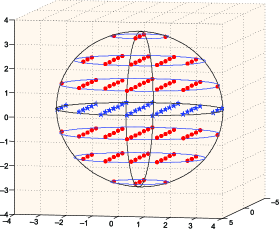
Figure 1: Lattice points in a ball of radius $R=\gamma d^{*}=3.2$ in the three dimensional space ($d^{*}=3$). Red points are those of $\mathcal{C}_{1}(d^{*},\gamma)\setminus\mathcal{C}_{2}(d^{*},\gamma)$ while blue stars are those of $\mathcal{C}_{2}(d^{*},\gamma)$. In this example, $N(d^{*},\gamma)=N(3,1.07)=110$.

In order to determine the asymptotic behavior of $N_{1}(d^{*},\gamma)$ and $N_{2}(d^{*},\gamma)$ when $d^{*}$ tends to infinity, we will rely on their integral representation through Jacobi’s $\theta$-function. Recall that the latter is given by $\mathsf{h}(z)=\sum_{r\in\mathbb{Z}}z^{r^{2}}$, which is well defined for any complex number $z$ belonging to the unit ball $|z|<1$. To briefly explain where the relation between $N_{i}(d^{*},\gamma)$ and the $\theta$-function comes from, let us denote by $\{a_{r}\}$ the sequence of coefficients of the power series of $\mathsf{h}(z)^{d^{*}}$, that is, $\mathsf{h}(z)^{d^{*}}=\sum_{r\geq 0}a_{r}z^{r}$. One easily checks that $\forall r\in\mathbb{N}$, $a_{r}=\operatorname{Card}\{\mathbf{k}\in\mathbb{Z}^{d^{*}}\dvtx k_{1}^{2}+\cdots+k_{d^{*}}^{2}=r\}$. Thus, for every $\gamma$ such that $\gamma d^{*}$ is integer, we have $N_{1}(d^{*},\gamma)=\sum_{r=0}^{\gamma d^{*}}a_{r}$. As a consequence of Cauchy’s theorem, we get

$$N_{1}\bigl{(}d^{*},\gamma\bigr{)}=\frac{1}{2\pi i}\oint\frac{\mathsf{h}(z)^{d^{*}}}{z^{\gamma d^{*}}}\frac{dz}{z(1-z)},$$

where the integral is taken over any circle $|z|=w$ with $0<w<1$. Exploiting this representation and applying the saddle-point method thoroughly described in Dieudonne , we get the following result.

Proposition 2

Let $\gamma>0$ be an integer and let $\mathsf{l}_{\gamma}(z)=\log{\mathsf{h}(z)}-\gamma\log z$.

[(1)]

There is a unique solution $z_{\gamma}$ in $(0,1)$ to the equation $\mathsf{l}_{\gamma}^{\prime}(z)=0$. Furthermore, the function $\gamma\mapsto z_{\gamma}$ is increasing and $\mathsf{l}_{\gamma}^{\prime\prime}(z)>0$.

For $i=1,2$, the following equivalences hold true:

$$N_{i}\bigl{(}d^{*},\gamma\bigr{)}=\biggl{(}\frac{\mathsf{h}(z_{\gamma})}{z_{\gamma}^{\gamma}}\biggr{)}^{d^{*}}\frac{1+o(1)}{\mathsf{h}(z_{\gamma})^{i-1}z_{\gamma}(1-z_{\gamma})(2\mathsf{l}_{\gamma}^{\prime\prime}(z_{\gamma})\pi d^{*})^{1/2}}$$

as $d^{*}$ tends to infinity.

Hereafter, it will be useful to note that the second part of Proposition 2 yields

$$\log\bigl{(}N_{1}\bigl{(}d^{*},\gamma\bigr{)}-N_{2}\bigl{(}d^{*},\gamma\bigr{)}\bigr{)}=d^{*}\mathsf{l}_{\gamma}(z_{\gamma})-\tfrac 12\log d^{*}+c_{\gamma}+o(1)$$

(12)

$$\eqntext{\mbox{as }d^{*}\to\infty,}$$ (13)

with $c_{\gamma}=\log(\frac{\mathsf{h}(z_{\gamma})-1}{\mathsf{h}(z_{\gamma})z_{\gamma}(1-z_{\gamma})\sqrt{2\pi\mathsf{l}^{\prime\prime}_{\gamma}(z_{\gamma})}})$. Furthermore, while the asymptotic equivalences of Proposition 2 are established for integer values of $\gamma>0$, relation $\log(N_{1}(d^{*},\gamma)-N_{2}(d^{*},\gamma))=d^{*}\mathsf{l}_{\gamma}(z_{\gamma})(1+o(1))$ holds true for any positive real number $\gamma$ Mazo . In order to get an idea of how the terms $z_{\gamma}$ and $\mathsf{l}_{\gamma}(z_{\gamma})$ depend on $\gamma$, we depicted in Figure 2 the plots of these quantities as functions of $\gamma>0$.

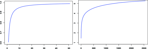
Figure 2: The plots of mappings $\gamma\mapsto z_{\gamma}$ and $\gamma\mapsto\mathsf{l}_{\gamma}(z_{\gamma})$. One can observe that both functions are increasing, the first one converges to $1$ very rapidly, while the second one seems to diverge very slowly.

Combining relation (4) with Theorem 1, we get the following result.

Corollary 3

Let condition [C1$(\kappa,L)$] be satisfied with some known constants $\kappa>0$ and $L<\infty$. Consider the asymptotic set-up in which both $d=d_{n}$ and $d^{*}=d^{*}_{n}$ tend to infinity as $n\to\infty$. Assume that $d$ grows at a sub-exponential rate in $n$, that is, $\log\log d=o(\log n)$. If

$$\limsup_{n\to\infty}\frac{d^{*}}{\log n}<\frac{2}{\mathsf{l}_{\gamma}(z_{\gamma})}$$

with $\gamma=L/\kappa$, then consistent estimation of $J$ is possible and can be achieved, for instance, by the estimator $\widehat{J}_{n}$.

5 Tightness of the assumptions

In this section, we focus our attention on the functional class $\Sigma(\kappa,L)$ of all functions satisfying assumption [C1($\kappa,L$)]. For emphasizing that $J$ is the sparsity pattern of the function $\mathsf{f}$, we write $J_{\mathsf{f}}$ instead of $J$. We assume that $s=\operatorname{Card}(J)=d^{*}$. The goal is to provide conditions under which the consistent estimation of the sparsity support is impossible, that is, there exists a constant $c>0$ and an integer $n_{0}\in\mathbb{N}$ such that, if $n\geq n_{0}$,

$$\inf_{\widetilde{J}}\sup_{\mathsf{f}\in\Sigma(\kappa,L)}\mathbf{P}_{\mathsf{f}}(\widetilde{J}\neq J_{\mathsf{f}})\geq c,$$

where the $\inf$ is over all possible estimators of $J_{\mathsf{f}}$. To this end, we introduce a set of $M+1$ probability distributions $\mu_{0},\ldots,\mu_{M}$ on $\Sigma(\kappa,L)$ and use the fact that

$$\inf_{\widetilde{J}}\sup_{\mathsf{f}\in\widetilde{\Sigma}(\kappa,L)}\mathbf{P}_{\mathsf{f}}(\widetilde{J}\neq J_{\mathsf{f}})\geq\inf_{\widetilde{J}}\frac{1}{M}\sum_{\ell=1}^{M}\int_{\Sigma(\kappa,L)}\mathbf{P}_{\mathsf{f}}(\widetilde{J}\neq J_{\mathsf{f}})\mu_{\ell}(d\mathsf{f}).$$ (14)

These measures $\mu_{\ell}$ will be chosen in such a way that for each $\ell\geq 1$ there is a set $J_{\ell}$ of cardinality $d^{*}$ such that $\mu_{\ell}\{J_{\mathsf{f}}=J_{\ell}\}=1$ and all the sets $J_{1},\ldots,J_{M}$ are distinct. The measure $\mu_{0}$ is the Dirac measure in $0$. Considering these $\mu_{\ell}$s as “priors” on $\Sigma(\kappa,L)$ and defining the corresponding “posteriors” $\mathbb{P}_{0},\mathbb{P}_{1},\ldots,\mathbb{P}_{M}$ by

$$\mathbb{P}_{\ell}(A)=\int_{\Sigma(\kappa,L)}\mathbf{P}_{\mathsf{f}}(A)\mu_{\ell}(d\mathsf{f})\qquad\mbox{for every measurable set }A\subset\mathbb{R}^{n},$$

we can write inequality (14) as

$$\inf_{\widetilde{J}}\sup_{\mathsf{f}\in\Sigma(\kappa,L)}\mathbf{P}_{\mathsf{f}}(\widetilde{J}\neq J_{\mathsf{f}})\geq\inf_{\psi}\frac{1}{M}\sum_{\ell=1}^{M}\mathbb{P}_{\ell}(\psi\not=\ell),$$ (15)

where the $\inf$ is taken over all random $\psi$ taking values in $\{0,\ldots,M\}$. The latter $\inf$ will be controlled using a suitable version of the Fano lemma. To state it, we denote by $\mathcal{K}(P,Q)$ the Kullback–Leibler divergence between two probability measures $P$ and $Q$ defined on the same probability space.

Lemma 4 ((Corollary 2.6 of Tsybakov09 ))

Let $M\geq 3$ be an integer, $(\mathcal{X},\mathcal{A})$ be a measurable space and let $P_{0},\ldots,P_{M}$ be probability measures on $(\mathcal{X},\mathcal{A})$. Let us set $\bar{p}_{e,M}=\inf_{\psi}M^{-1}\sum_{\ell=1}^{M}P_{\ell}(\psi\not=\ell)$, where the $\inf$ is taken over all measurable functions $\psi\dvtx\mathcal{X}\to\{1,\ldots,M\}$. If for some $0<\alpha<1$, $\frac{1}{M+1}\sum_{\ell=1}^{M}\mathcal{K}(P_{\ell},\break P_{0})\leq\alpha\log M$, then $\bar{p}_{e,M}\geq\frac{1}{2}-\alpha$.

We apply this lemma with $\mathcal{X}$ being the set of all arrays $\mathbf{y}=\{y_{\mathbf{k}}\dvtx\mathbf{k}\in\mathbb{Z}^{d}\}$ such that for some $K>0$ the entries $y_{\mathbf{k}}=0$ for every $\mathbf{k}$ larger than $K$ in $\ell_{2}$-norm. It follows from Fano’s lemma that one can deduce a lower bound on $\bar{p}_{e,M}$, the quantity we are interested in, from an upper bound on the average Kullback–Leibler divergence between $\mathbb{P}_{\ell}$ and $\mathbb{P}_{0}$. With these tools at hand, we are in a position to state the main result on the impossibility of consistent estimation of the sparsity pattern in the case when the conditions of Theorem 1 are violated.

Theorem 2

Assume that $\vartheta=L/\kappa>1$ and $({{d}\atop{d^{*}}})\geq 3$. Let $\gamma_{\vartheta}$ be the largest integer satisfying $\gamma(1+(\mathsf{h}(z_{\gamma})-1)^{-1})\leq\vartheta$, where the Jacobi $\theta$-function $\mathsf{h}$ and $z_{\gamma}$ are those defined in Section 4. [(ii)]

If for some $\alpha\in(0,1/2)$,

$$\frac{N(d^{*},\gamma_{\vartheta})d^{*}\log(d/d^{*})}{n^{2}}\geq\frac{\vartheta}{\alpha\gamma_{\vartheta}}\kappa^{2},$$ (16)

then, for $d^{*}$ large enough, $\inf_{\widetilde{J}}\sup_{\mathsf{f}\in\Sigma}\mathbf{P}_{\mathsf{f}}(\widetilde{J}\neq J_{\mathsf{f}})\geq\frac{1}{2}-\alpha$.

If for some $\alpha\in(0,1/2)$,

$$\frac{d^{*}\log(d/d^{*})}{n}\geq\frac{\kappa}{\alpha},$$ (17)

then $\inf_{\widetilde{J}}\sup_{\mathsf{f}\in\Sigma}\mathbf{P}_{\mathsf{f}}(\widetilde{J}\neq J_{\mathsf{f}})\geq\frac{1}{2}-\alpha$.

It is worth stressing here that condition (16) is the converse of condition (9) of Theorem 1 in the case $d^{*}\to\infty$, in the sense that condition (9) amounts to requiring that the left-hand side of (16) is smaller than some constant. There is, however, one difference between the quantities involved in these conditions: the term $N(d^{*},\vartheta(1+\tau))$ of (9) is replaced by $N(d^{*},{\gamma_{\vartheta}})$ in condition (16). One can wonder how close ${\gamma_{\vartheta}}$ is to $\vartheta$. To give a qualitative answer to this question, we plotted in Figure 3 the curve of the mapping $\vartheta\mapsto{\gamma_{\vartheta}}$ along with the bisector $\vartheta\mapsto\vartheta$. We observe that the difference between two curves is small compared to $\vartheta$. As we discuss it later, this property shows that the constants involved in the necessary condition and in the sufficient condition for consistent estimation of $J$ are very close, especially for large values of $\vartheta$.

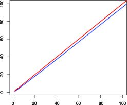
Figure 3: The curve of the function $L\mapsto{\gamma_{L}}$ (blue) and the bisector (red).

6 Adaptivity and minimax rates of separation

6.1 Adaptation with respect to $L$ and $\kappa$

The estimator $\widehat{J}(\mathbf{m},\bolds{\lambda})$ we have introduced in Section 3 is clearly nonadaptive: the tuning parameters $(\mathbf{m},\bolds{\lambda})$ recommended by the developed theory involve the values $L$ and $\kappa$, which are generally unknown. Fortunately, we can take advantage of the fact that the choice of $\mathbf{m}$ and $\bolds{\lambda}$ is governed by the one-dimensional parameter $\vartheta=L(1+\tau)/\kappa$. Therefore, it is realistic to assume that a finite grid of values $1<\vartheta_{1}\leq\cdots\leq\vartheta_{K}<\infty$ is available containing a true value of $\vartheta$. The following result provides an adaptive procedure of variable selection with guaranteed control of the error.

Proposition 5

Let $1<\vartheta_{1}\leq\cdots\leq\vartheta_{K}<\infty$ and $\tau>0$ be given values, and set

$$i^{*}=\min\biggl{\{}i\dvtx(1+\tau)\frac{\max_{j=1,\ldots,d}\sum_{\mathbf{k}\in\mathbb{Z}^{d}}k_{j}^{2}\theta_{\mathbf{k}}^{2}}{\min_{j\in J}\sum_{\mathbf{k}\dvtx k_{j}\neq 0}\theta_{\mathbf{k}}^{2}}\leq\vartheta_{i}\biggr{\}}\leq K.$$

For every $i,\ell\in\mathbb{N}$, let us denote $\widehat{J}_{n}(i)=\widehat{J}_{n}(\mathbf{m}(\vartheta_{i}),\bolds{\lambda}(\vartheta_{i}))$ with $m_{\ell}(\vartheta)=(\vartheta\ell)^{1/2}$ and

$$\lambda_{\ell}(\vartheta)=\frac{2\sqrt{2N(\ell,\vartheta)d^{*}\log(2ed/d^{*})}+4d^{*}\log(2ed/d^{*})}{n}.$$

If the condition $4\lambda_{s}(\vartheta_{i^{*}})<\kappa\tau/(1+\tau)$ is fulfilled, then the estimator $\widehat{J}_{n}^{\mathrm{ad}}=\bigcup_{i=1}^{K}\widehat{J}_{n}(i)$ satisfies $\mathbf{P}(\widehat{J}_{n}^{\mathrm{ad}}\not=J)\leq(K+2)(d^{*}/2ed)^{d^{*}}$.

In simple words, if the grid of possible values $\{\vartheta_{i}\}$ has a cardinality $K$ which is not too large [i.e., $K(d^{*}/d)^{d^{*}}\to 0$], then declaring a variable relevant if at least one of the procedures $\widehat{J}_{n}(i)$ suggests its relevance provides a consistent and adaptive variable selection strategy. The proof of this statement follows immediately from Proposition 1 and Theorem 1. Indeed, applying Proposition 1 with $A=2$ yields $\mathbf{P}(\widehat{J}_{n}^{\mathrm{ad}}\not\subset J)\leq\sum_{i=1}^{K}\mathbf{P}(\widehat{J}_{n}(i)\not\subset J)\leq K(d^{*}/2ed)^{d^{*}}$, while Theorem 1 ensures that $\mathbf{P}(\widehat{J}_{n}^{\mathrm{ad}}\not\supset J)\leq\mathbf{P}(\widehat{J}_{n}(i^{*})\not\supset J)\leq 2(d^{*}/2ed)^{d^{*}}$.

6.2 Minimax rates of separation

Since the methodology of Section 3 takes its roots in the theory of hypotheses testing, one naturally wonders what are the minimax rates of separation in the problem of variable selection. The results stated in foregoing sections allow us to answer this question in the case of Sobolev smoothness 1 and alternatives separated in $L^{2}$-norm. The following result, the proof of which is postponed to the Appendix E provides minimax rates. We assume herein that the true sparsity $s=\operatorname{Card}(J)$ and its known upper estimate $d^{*}$ are such that $d^{*}/s$ is bounded from above by some constant.

Proposition 6

There is a constant $D^{*}$ depending only on $L$ such that if

$$\kappa\geq D^{*}\biggl{\{}\biggl{(}\frac{\log(d/s)}{n^{2}}\biggr{)}^{2/(4+s)}\vee\frac{s\log(d/s)}{n}\biggr{\}},$$

then there exists a consistent estimator of $J$. Furthermore, the consistency is uniform in $\mathsf{f}\in\Sigma(\kappa,L)$. On the other hand, there is a constant $D_{*}$ depending only on $L$ such that if

$$\kappa\leq D_{*}\biggl{\{}\biggl{(}\frac{\log(d/s)}{n^{2}}\biggr{)}^{2/(4+s)}\vee\frac{s\log(d/s)}{n}\biggr{\}},$$

then uniformly consistent estimation of $J$ is impossible.

Borrowing the terminology of the theory of hypotheses testing, we say that $(\frac{\log(d/s)}{n^{2}})^{2/(4+s)}\vee\frac{s\log(d/s)}{n}$ is the minimax rate of separation in the problem of variable selection for Sobolev smoothness one. These results readily extend to Sobolev smoothness of any order $\beta\geq 1$, in which case the rate of separation takes the form $(\frac{\log(d/s)}{n^{2}})^{2\beta/(4\beta+s)}\vee\frac{s\log(d/s)}{n}$. The first term in this maximum coincides, up to the logarithmic term, with the minimax rate of separation in the problem of detection of an $s$-dimensional signal IngsterStepanova11 . Note, however, that in our case this logarithmic inflation is unavoidable. It is the price to pay for not knowing in advance which $s$ variables are relevant.

7 Nonparametric regression with random design

So far, we have analyzed the situation in which noisy observations of the regression function $\mathsf{f}(\cdot)$ are available at all points $\mathbf{x}\in[0,1]^{d}$. Let us turn now to the more realistic model of nonparametric regression, when the observed noisy values of $\mathsf{f}$ are sampled at random in the unit hypercube $[0,1]^{d}$. More precisely, we assume that $n$ independent and identically distributed pairs of input-output variables $(\mathbf{X}_{i},Y_{i})$, $i=1,\ldots,n$ are observed that obey the regression model

$$Y_{i}=\mathsf{f}(\mathbf{X}_{i})+\sigma\varepsilon_{i},\qquad i=1,\ldots,n.$$

The input variables $\mathbf{X}_{1},\ldots,\mathbf{X}_{n}$ are assumed to take values in $\mathbb{R}^{d}$ while the output variables $Y_{1},\ldots,Y_{n}$ are scalar. As usual, $\varepsilon_{1},\ldots,\varepsilon_{n}$ are such that $\mathbf{E}[\varepsilon_{i}|\mathbf{X}_{i}]=0$, $i=1,\ldots,n$; additional conditions will be imposed later. Without requiring from $\mathsf{f}$ to be of a special parametric form, we aim at recovering the set $J\subset\{1,\ldots,d\}$ of its relevant variables. The noise magnitude $\sigma$ is assumed to be known.

It is clear that the estimation of $J$ cannot be accomplished without imposing some further assumptions on $\mathsf{f}$ and on the distribution $P_{X}$ of the input variables. Roughly speaking, we will assume that $\mathsf{f}$ is differentiable with a squared integrable gradient and that $P_{X}$ admits a density which is bounded from below. More precisely, let $\mathsf{g}$ denote the density of $P_{X}$ w.r.t. the Lebesgue measure. [[C2]]

$\mathsf{g}(\mathbf{x})=0$ for any $\mathbf{x}\notin[0,1]^{d}$ and that $\mathsf{g}(\mathbf{x})\geq{g_{\min}}$ for any $\mathbf{x}\in[0,1]^{d}$.

The next assumptions imposed to the regression function and to the noise require their boundedness in an appropriate sense. These assumptions are needed in order to prove, by means of a concentration inequality, the closeness of the empirical coefficients to the true ones. [[C3]]

The $L^{\infty}([0,1]^{d},\mathbb{R},P_{X})$ and $L^{2}([0,1]^{d},\mathbb{R},P_{X})$ norms of the function $\mathsf{f}$ are bounded from above, respectively, by $L_{\infty}$ and $L_{2}$, that is, $\mathbf{P}(|\mathsf{f}(\mathbf{X})|\leq L_{\infty})=1$ and $\mathbf{E}[\mathsf{f}(\mathbf{X})^{2}]\leq L_{2}^{2}$.

The noise variables satisfy a.e. $\mathbf{E}[e^{t\varepsilon_{i}}|\mathbf{X}_{i}]\leq e^{t^{2}/2}$ for all $t>0$.

We stress once again that the primary aim of this work is merely to understand when it is possible to consistently estimate the sparsity pattern. The estimator that we will define is intended to show the possibility of consistent estimation, rather than being a practical procedure for recovering the sparsity pattern. Therefore, the estimator will be allowed to depend on the parameters $g_{\min}$, $L$, $\kappa$ and $L_{2}$ appearing in conditions [C1]–[C3].

7.1 An estimator of $J$ and its consistency

The estimator of the sparsity pattern $J$ that we are going to introduce now is based on the following simple observation: if $j\notin J$, then $\theta_{\mathbf{k}}[\mathsf{f}]=0$ for every $\mathbf{k}$ such that $k_{j}\not=0$. In contrast, if $j\in J$, then there exists $\mathbf{k}\in\mathbb{Z}^{d}$ with $k_{j}\not=0$ such that $|\theta_{\mathbf{k}}[\mathsf{f}]|>0$. To turn this observation into an estimator of $J$, we start by estimating the Fourier coefficients $\theta_{\mathbf{k}}[\mathsf{f}]$ by their empirical counterparts,

$$\widehat{\theta}_{\mathbf{k}}=\frac{1}{n}\sum_{i=1}^{n}\frac{\varphi_{\mathbf{k}}(\mathbf{X}_{i})}{\mathsf{g}(\mathbf{X}_{i})}Y_{i},\qquad\mathbf{k}\in\mathbb{Z}^{d}.$$

Then, for every $\ell\in\mathbb{N}$ and for any $\gamma>0$, we introduce the notation $S^{j}_{m,\ell}=\{\mathbf{k}\in\mathbb{Z}^{d}\dvtx\|\mathbf{k}\|_{2}\leq m,\|\mathbf{k}\|_{0}\leq\ell,k_{j}\neq 0\}$. The estimator of $J$ is defined by

$$\widehat{J}_{n}^{(1)}(m,\lambda)=\bigl{\{}j\in\{1,\ldots,d\}\dvtx\operatorname{max}_{\mathbf{k}\in S_{m,d^{*}}^{j}}|\widehat{\theta}_{\mathbf{k}}|>{\lambda}\bigr{\}},$$ (18)

where $m$ and ${\lambda}$ are some parameters to be defined later. The next result, the proof of which is placed in the supplementary material CDsupp , provides consistency guarantees for $\widehat{J}_{n}^{(1)}(m,\lambda)$.

Theorem 3

Let conditions [C1]–[C4] be fulfilled with some known values $g_{\min}$, $\vartheta=2L/\kappa$ and $L_{2}$. Assume furthermore that the design density $\mathsf{g}$ and an upper estimate on the noise magnitude $\sigma$ are available. Set $m=(\vartheta d^{*})^{1/2}$ and $\lambda=4(\sigma+L_{2})({d^{*}\log(24\sqrt{\vartheta}d/d^{*})}/{ng_{\min}^{2}})^{1/2}$. If the following conditions are satisfied:

$$\frac{d^{*}\log(24\sqrt{\vartheta}d/d^{*})}{n} \leq \frac{L_{2}^{2}}{L_{\infty}^{2}},$$

$$\frac{128({\sigma}+L_{2})^{2}d^{*}N(d^{*},\vartheta)\log(24\sqrt{\vartheta}d/d^{*})}{ng_{\min}^{2}} < \kappa,$$

then the estimator $\widehat{J}^{(1)}(m,\lambda)$ satisfies $\mathbf{P}(\widehat{J}^{(1)}(m,\lambda)\neq J)\leq(8d/d^{*})^{-d^{*}}$.

If we take a look at the conditions of Theorem 3 ensuring the consistency of $\widehat{J}_{n}^{(1)}$, it becomes clear that the strongest requirement is the second inequality in (3). Roughly speaking, this condition requires that $d^{*}N(d^{*},\vartheta)\log(d/d^{*})/n$ is bounded from above by some constant. According to results stated in Section 4, $N(d^{*},\vartheta)$ diverges exponentially fast, making inequality (3) impossible for $d^{*}$ larger than $\log n$ up to a multiplicative constant.

It is also worth stressing that although we require the $P_{X}$-a.e. boundedness of $\mathsf{f}$ by some constant $L_{\infty}$, this constant is not needed for computing the estimator proposed in Theorem 3. Only constants related to some quadratic functionals of the sequence of Fourier coefficients $\theta_{\mathbf{k}}[\mathsf{f}]$ are involved in the tuning parameters $m$ and $\lambda$. This point might be important for designing practical estimators of $J$, since the estimation of quadratic functionals is more realistic (see, e.g., LaurentMassart , Cai06 ) than the estimation of $\sup$-norm.

Theorem 3 can be reformulated to characterize the level of relevance $\kappa$ for the relevant components of $\mathbf{X}$ making their identification possible. In fact, an alternative way of stating Theorem 3 is the following: under conditions [C1]–[C4] if $\vartheta$ is an arbitrary tuning parameter satisfying the first inequality in (3), then the estimator $\widehat{J}_{n}^{(1)}(m,\lambda)$—with $m$ and $\lambda$ chosen as in Theorem 3—satisfies $\mathbf{P}(\widehat{J}_{n}^{(1)}(m,\lambda)\not=J)\leq(8d/d^{*})^{-d^{*}}$ if the smallest level of relevance $\kappa$ for components $X_{j}$ of $\mathbf{X}$ with $j\in J$ is not smaller than $8\lambda^{2}N(d^{*},m^{2}/d^{*})$. This statement can be easily deduced from the proof of Theorem 3; cf. the supplementary material CDsupp .

7.2 Tightness of the assumptions

A natural question is now to check that the assumptions of Theorem 3 are tight in the asymptotic regimes of fixed sparsity and increasing ambient dimension, as well as increasing sparsity. We will only establish an analogue of claim (ii) of Theorem 2. An attempt to prove a result similar to claim (i) of Theorem 2 was done in ComDal11 , Theorem 2. However, the result of ComDal11 involves a stringent assumption on the empirical Gram matrix (cf. condition (6) in ComDal11 ) and, unfortunately, we are unable to prove the existence of a sampling scheme for which this assumption is fulfilled.

We assume that the errors $\varepsilon_{i}$ are i.i.d. standard Gaussian, and we focus our attention on the functional class $\Sigma(\kappa,L)$. The following simple result shows that the conditions of Theorem 3 are tight in the case of fixed intrinsic dimension.

Proposition 7

Let the design $\mathbf{X}_{1},\ldots,\mathbf{X}_{n}\in[0,1]^{d}$ be either deterministic or random. If for some positive $\alpha<1/2$, the inequality

$$\frac{d^{*}\log(d/d^{*})}{n}\geq\kappa\alpha^{-1}$$

holds true, then there is a constant $c\!>\!0$ such that $\inf_{\widetilde{J}_{n}}\sup_{\mathsf{f}\in\Sigma(\kappa,L)}\!\mathbf{P}_{\mathsf{f}}(\widetilde{J}_{n}\!\neq\!J_{\mathsf{f}})\!\geq\!c$.

8 Concluding remarks

The results proved in previous sections almost exhaustively answer the questions on the existence of consistent estimators of the sparsity pattern in the model of Gaussian white noise and, to a smaller extent, in nonparametric regression. In fact as far as only rates of convergence are of interest, the result obtained in Theorem 1 is shown in Section 5 to be unimprovable. Thus only the problem of finding sharp constants remains open. To make these statements more precise, let us consider the simplified set-up $\sigma=\kappa=1$ and define the following two regimes:

• The regime of fixed sparsity, that is, when the sample size $n$ and the ambient dimension $d$ tend to infinity but the intrinsic dimension $d^{*}$ remains constant or bounded.

• The regime of increasing sparsity, that is, when the intrinsic dimension $d^{*}$ tends to infinity along with the sample size $n$ and the ambient dimension $d$. For simplicity, we will assume that $d^{*}=O(d^{1-\varepsilon})$ for some $\varepsilon>0$.

In the fixed sparsity regime, in view of Theorems 1 and 3, consistent estimation of the sparsity pattern can be achieved both in the Gaussian white noise model and nonparametric regression as soon as $\limsup_{n\to\infty}(d^{*}\log d)/n<c_{\star}$, where $c_{\star}$ is the constant defined by $c_{*}=1/8$ for the Gaussian white noise model and

$$c_{\star}=\min\biggl{(}\frac{L_{2}^{2}}{2L_{\infty}^{2}},\frac{g_{\min}^{2}}{2^{8}(1+L_{2})^{2}N(d^{*},2L)}\biggr{)}$$

for the regression model. On the other hand, by Theorem 2 and Proposition 7, consistent estimation of the sparsity pattern is impossible if$\liminf_{n\to\infty}(d^{*}\log d)/n>c^{\star}$ with $c^{\star}=2$. Thus, up to multiplicative constants $c_{\star}$ and $c^{\star}$ (which are clearly not sharp), the results of Theorems 1 and 3 cannot be improved in the regime of fixed sparsity.

In the regime of increasing sparsity, the results we get in the model of Gaussian white noise are much stronger than those for nonparametric regression. In the former model, taking the logarithm of both sides of inequality (9) and using formula (4) for $N(d^{*},\cdot)=N_{1}(d^{*},\cdot)-N_{2}(d^{*},\cdot)$, we see that consistent estimation of $J$ is possible when, for some $\tau>0$ and for all $n$, the following two conditions are fulfilled:

$$\cases{\mathsf{l}_{L+\tau}(z_{L+\tau})d^{*}+\frac{1}{2}\log d^{*}+\log\log\bigl{(}d/d^{*}\bigr{)}-2\log n<\underline{c}_{1},\vspace*{2pt}\cr\log d^{*}+\log\log\bigl{(}d/d^{*}\bigr{)}-\log n\leq\underline{c}^{\prime}_{1}}$$ (20)

with some constants $\underline{c}_{1}=\underline{c}_{1}(L,\tau)$ and $\underline{c}_{1}^{\prime}=\underline{c}_{1}^{\prime}(L,\tau)$. On the other hand, Theorem 2 yields that there are some constants $\bar{c}_{1}$ and $\bar{c}_{1}^{\prime}$ such that it is impossible to consistently estimate $J$ if either one of the conditions

$$\mathsf{l}_{{\gamma_{L}}}(z_{{\gamma_{L}}})d^{*}+\tfrac 12\log d^{*}+\log\log\bigl{(}d/d^{*}\bigr{)}-2\log n \geq \bar{c}_{1},$$ (21)

$$\log d^{*}+\log\log\bigl{(}d/d^{*}\bigr{)}-\log n \geq \bar{c}^{\prime}_{1},$$ (22)

is satisfied. First note that the left-hand side of the second condition in (20) is exactly the same as the left-hand side of (22). If we compare now the left-hand side of the first condition in (20) with the left-hand side of (21), we see that only the coefficients of $d^{*}$ differ. To measure the degree of difference of these two coefficients we draw in Figure 4 the plots of the functions $L\mapsto\mathsf{l}_{L}(z_{L})$ and $L\mapsto\mathsf{l}_{{\gamma_{L}}}(z_{{\gamma_{L}}})$, with ${\gamma_{L}}$ as is Theorem 2. One can observe that the two curves are very close, especially for relatively large values of $L$. This implies that the conditions in (20) are tight. A simple consequence of inequalities (20) and (21) is that the consistent recovery of the sparsity pattern is possible under the condition $d^{*}/\log n\to 0$ and impossible for $d^{*}/\log n\to\infty$ as $n\to\infty$, provided that $\log\log(d/d^{*})=o(\log n)$.

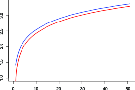
Figure 4: The curves of functions $L\mapsto\mathsf{l}_{L}(z_{L})$ (blue curve) and $L\mapsto\mathsf{l}_{{\gamma_{L}}}(z_{{\gamma_{L}}})$ (red curve).

Still in the regime of increasing sparsity, but for nonparametric regression, we proved that consistent estimation of the sparsity pattern is possible whenever

$$\cases{\mathsf{l}_{L+\tau}(z_{L+\tau})d^{*}+\frac{1}{2}\log d^{*}+\log\log\bigl{(}d/d^{*}\bigr{)}-\log n<\underline{c}_{2},\vspace*{2pt}\cr\log d^{*}+\log\log d-\log n<\underline{c}^{\prime}_{2}}$$ (23)

with some constants $\underline{c}_{2}=\underline{c}_{2}(g_{\min},\sigma,L_{2},L)$ and $\underline{c}^{\prime}_{2}=2\log(L_{2}/L_{\infty})$. As we have already mentioned, the second condition in (23) is tight, up to the choice of $\underline{c}_{2}^{\prime}$, in view of Proposition 7. It is natural to expect that the first condition is tight as well, since it is in the model of Gaussian white noise, which has the reputation of being simpler than the model of nonparametric regression. However, we do not have a mathematical proof of this statement.

Let us stress now that, all over this work, we have deliberately avoided any discussion on the computational aspects of the variable selection in nonparametric regression. The goal in this paper was to investigate the possibility of consistent recovery without paying attention to the complexity of the selection procedure. This lead to some conditions that could be considered a benchmark for assessing the properties of sparsity pattern estimators. As for the estimators proposed in Section 3, it is worth noting that their computational complexity is not always prohibitively large. A recommended strategy is to compute the coefficients $\widehat{\theta}_{\mathbf{k}}$ in a stepwise manner; at each step $K=1,2,\ldots,d^{*}$ only the coefficients $\widehat{\theta}_{\mathbf{k}}$ with $\|\mathbf{k}\|_{0}=K$ need to be computed and compared with the threshold. If some $\widehat{\theta}_{\mathbf{k}}$ exceeds the threshold, then all the variables $X^{j}$ corresponding to nonzero coordinates of $\mathbf{k}$ are considered as relevant. We can stop this computation as soon as the number of variables classified as relevant attains $d^{*}$. While the worst-case complexity of this procedure is exponential, there are many functions $\mathsf{f}$ for which the complexity of the procedure will be polynomial in $d$. For example, this is the case for additive models in which $\mathsf{f}(\mathbf{x})=\mathsf{f}_{1}(x_{i_{1}})+\cdots+\mathsf{f}_{d^{*}}(x_{i_{d^{*}}})$ for some univariate functions $\mathsf{f}_{1},\ldots,\mathsf{f}_{d^{*}}$.

Note also that in the present study we focused exclusively on the consistency of variable selection without paying any attention to the consistency of regression function estimation. A thorough analysis of the latter problem being left to a future work, let us simply remark that in the case of fixed $d^{*}$, under the conditions of Theorem 3, it is straightforward to construct a consistent estimator of the regression function. In fact, it suffices to use a projection estimator with a properly chosen truncation parameter on the set of relevant variables. The situation is much more delicate in the case when the sparsity $d^{*}$ grows to infinity along with the sample size $n$. Presumably, condition (20) is no longer sufficient for consistently estimating the regression function. The rationale behind this conjecture is that the minimax rate of convergence for estimating $\mathsf{f}$ in our context, if we assume in addition that the set of relevant variables is known, is equal to $n^{-2/(2+d^{*})}=\exp(-2\log n/(2+d^{*}))$. If the left-hand side of (20) is equal to a constant and $\log\log d=o(\log n)$, then the aforementioned minimax rate does not tend to zero, making thus the estimator inconsistent.

Finally, we would like to mention that the selection of relevant variables is a challenging statistical task, which might be useful to perform independently of the task of regression function estimation. Indeed, if we succeed in identifying relevant variables on a data-set having a small sample size, we can continue the data collection process more efficiently by recording only the values of relevant variables. This may considerably reduce the memory costs related to the data storage and the financial costs necessary for collecting new data. Then, the regression function may be estimated more accurately on the base of this new (larger) data-set.

Appendix A Proof of Proposition 1

To ease notation, we write $\widehat{J}_{n}$ instead of $\widehat{J}_{n}(\mathbf{m},\bolds{\lambda})$. It is clear that $\widehat{J}_{n}\not\subset J$ if and only if $\exists j\in J^{c}$ such that $\max_{\ell\leq d^{*}}\lambda_{\ell}^{-1}\max_{I\in P_{\ell}^{d}}\widehat{Q}_{m,I}^{j}\geq 1$, where $Q_{m,I}^{j}=\sum_{\mathbf{k}\in S_{m,I}^{j}}\theta_{\mathbf{k}}^{2}$. For every $j\in\{1,\ldots,d\}$, let us set $R_{m,I}^{j}=\sum_{\mathbf{k}\in S_{m,I}^{j}}(\xi_{\mathbf{k}}^{2}-1)$ and $N_{m,I}^{j}=(Q_{m,I}^{j})^{-1/2}\sum_{\mathbf{k}\in S_{m,I}^{j}}\theta_{\mathbf{k}}\xi_{\mathbf{k}}$ so that

$$\widehat{Q}_{m,I}^{j}=\sum_{\mathbf{k}\in S_{m,I}^{j}}\biggl{(}y_{\mathbf{k}}^{2}-\frac{1}{n}\biggr{)}=Q_{m,I}^{j}+\frac{2\sqrt{Q_{m,I}^{j}}}{\sqrt{n}}N_{m,I}^{j}+\frac{1}{n}R_{m,I}^{j}.$$ (24)

For $j\in J^{c}$, the first two terms of the last sum vanish and, therefore, we have

$$\{\widehat{J}_{n}\not\subset J\}=\bigcup_{j\in J^{c}}\bigcup_{\ell\leq d^{*}}\bigcup_{I\in P_{\ell}^{d}}\bigl{\{}R_{m,I}^{j}\geq n\lambda_{\ell}\bigr{\}}=\bigcup_{\ell\leq d^{*}}\bigcup_{I\in P_{\ell}^{d}}\bigcup_{j\in J^{c}\cap I}\bigl{\{}R_{m,I}^{j}\geq n\lambda_{\ell}\bigr{\}},$$

where the last equality results from the fact that $R^{j}_{m,I}=0$ if $j\notin I$. The random variable $R^{j}_{m,I}$, being a centered sum of squares of independent standard Gaussian random variables, follows a translated $\chi^{2}$-distribution. The tails of this distribution can be evaluated using the following result.

Lemma 8 ((cf. Lemma 1 in LaurentMassart ))

Let $\xi_{1},\ldots,\xi_{D}$ be independent standard Gaussian random variables. For every $x\geq 0$ and for every vector $\mathbf{a}=(a_{1},\ldots,a_{D})\in\mathbb{R}^{D}_{+}$, the following inequalities hold true:

$$\mathbf{P}\Biggl{(}\sum_{i=1}^{D}a_{i}\bigl{(}\xi_{i}^{2}-1\bigr{)}\geq 2\|\mathbf{a}\|_{2}\sqrt{x}+2\|\mathbf{a}\|_{\infty}x\Biggr{)} \leq \exp(-x),$$

$$\mathbf{P}\Biggl{(}\sum_{i=1}^{D}a_{i}\bigl{(}\xi_{i}^{2}-1\bigr{)}\leq-2\|\mathbf{a}\|_{2}\sqrt{x}\Biggr{)} \leq \exp(-x).$$

We apply this lemma to $R^{i}_{m_{\ell},I}$, for which $\|\mathbf{a}\|_{\infty}=1$ and $\|\mathbf{a}\|_{2}^{2}={N(\ell,m_{\ell}^{2}/\ell)}$. Setting $n\lambda_{\ell}=2\sqrt{N(\ell,m_{\ell}^{2}/\ell)x}+2x$ and using the union bound, we get

$$\mathbf{P}(\widehat{J}_{n}\not\subset J) \leq \mathbf{P}\Biggl{(}\bigcup_{\ell=1}^{d^{*}}\Bigl{\{}\max_{I\in P_{\ell}^{d};i\in I}R^{i}_{m_{\ell},I}\geq n\lambda_{\ell}\Bigr{\}}\Biggr{)}$$

$$\leq \sum_{\ell=1}^{d^{*}}\ell\operatorname{Card}\bigl{(}P_{\ell}^{d}\bigr{)}\max_{I\in P_{\ell}^{d};i\in I}\mathbf{P}\bigl{(}R^{i}_{m_{\ell},I}>n\lambda_{\ell}\bigr{)}\leq e^{-x}\sum_{\ell=1}^{d^{*}}\ell\pmatrix{{d}\cr{\ell}}.$$

One checks that $\sum_{\ell=1}^{d^{*}}\ell({{d}\atop{\ell}})\leq(2ed/d^{*})^{d^{*}}$ holds true for every pair of integers $(d^{*},d)$ such that $1\leq d^{*}\leq d$; cf. the supplementary material CDsupp for a proof. Hence, for $x=Ad^{*}\log(2ed/d^{*})$, we get $\mathbf{P}(\widehat{J}_{n}\not\subset J)\leq(2ed/d^{*})^{-(A-1)d^{*}}$.

Appendix B Proof of Theorem 1

We begin with proving a stronger result that implies the claim of Theorem 1.

Proposition 9

Let $\alpha$ be a real number from $(0,1)$. If for every $j\in J$ and for $s=\operatorname{Card}(J)$ the inequality

$$Q_{m_{s},J}^{j}\geq\biggl{\{}\biggl{[}\lambda_{s}+\frac{2\sqrt{N(s,m_{s}^{2}/s)\log(2s/\alpha)}+1}{n}\biggr{]}^{1/2}+\biggl{[}\frac{2\log(2s/\alpha)}{n}\biggr{]}^{1/2}\biggr{\}}^{2}$$ (25)

holds true, then $\mathbf{P}(J\not\subset\widehat{J}_{n})\leq\alpha$.

To bound from above the probability of type II error, we rely on the equivalence: $J\not\subset\widehat{J}_{n}$ if and only if $\exists j\in J$ such that$\max_{\ell\leq d^{*}}\lambda_{\ell}^{-1}\max_{I\in P_{\ell}^{d}}\widehat{Q}_{m,I}^{j}\leq 1$. Recall that $s=\operatorname{Card}(J)$. Using Bonferroni’s inequality, we get

$$\mathbf{P}(J\not\subset\widehat{J}_{n}) \leq \sum_{j\in J}\mathbf{P}\Bigl{(}\max_{\ell\leq d^{*}}\lambda_{\ell}^{-1}\max_{I\in P_{\ell}^{d}}\widehat{Q}_{m,I}^{j}\leq 1\Bigr{)}$$

$$\leq \sum_{j\in J}\mathbf{P}\bigl{(}\widehat{Q}_{m_{s},J}^{j}\leq\lambda_{s}\bigr{)}\leq s\max_{j\in J}\mathbf{P}\bigl{(}\widehat{Q}_{m_{s},J}^{j}\leq\lambda_{s}\bigr{)}.$$

By virtue of decomposition (24),

$$\mathbf{P}\bigl{(}\widehat{Q}_{m_{s},J}^{j}\leq\lambda_{s}\bigr{)}=\mathbf{P}\biggl{(}\biggl{(}{\sqrt{Q_{m_{s},J}^{j}}}+\frac{1}{\sqrt{n}}N_{m_{s},J}^{j}\biggr{)}^{2}+\frac{1}{n}\bigl{(}R_{m_{s},J}^{j}-\bigl{(}N_{m_{s},J}^{j}\bigr{)}^{2}\bigr{)}\leq\lambda_{s}\biggr{)}.$$

One checks that $R_{m_{s},J}^{j}-(N_{m_{s},J}^{j})^{2}+N(s,m_{s}^{2}/s)$ is a drawn from $\chi^{2}$-distribution with $N(s,m_{s}^{2}/s)-1$ degrees of freedom. Therefore, using Lemma 8 stated in previous section, we get $\mathbf{P}(\frac{1}{n}(R_{m_{s},J}^{j}-(N_{m_{s},J}^{j})^{2})+\frac{1}{n}\leq\break-2\sqrt{N(s,m_{s}^{2}/s)\log(2s/\alpha)})\leq\frac{\alpha}{2s}$. Therefore, $\mathbf{P}(\widehat{Q}_{m_{s},J}^{j}\leq\lambda_{s})$ is upper-bounded by

$$\frac{\alpha}{2s}+\mathbf{P}\biggl{(}\biggl{(}{\sqrt{Q_{m_{s},J}^{j}}}+\frac{1}{\sqrt{n}}N_{m_{s},J}^{j}\biggr{)}^{2}\leq\lambda_{s}+\frac{2\sqrt{N(s,m_{s}^{2}/s)\log(2s/\alpha)}+1}{n}\biggr{)}.$$

Using the condition of the proposition, we get $\mathbf{P}(\widehat{Q}_{m_{s},J}^{j}\leq\lambda_{s})\leq\frac{\alpha}{2s}+\break\mathbf{P}(N_{m_{s},J}^{j}\leq-\sqrt{2\log(2s/\alpha)})\leq\frac{\alpha}{s}$. Combining this inequality with (B), we get the result of Proposition 9.

To deduce the claim of Theorem 1 from that of Proposition 9, we use the following lower bound:

$$Q_{m_{s},J}^{j} = Q^{j}-\sum_{j\in\mathop{\operatorname{supp}}(\mathbf{k})\subset J}\theta_{\mathbf{k}}^{2}\mathbf{1}_{\{\|\mathbf{k}\|_{2}\geq m_{s}\}}\geq\kappa-\sum_{j\in\mathop{\operatorname{supp}}(\mathbf{k})\subset J}\theta_{\mathbf{k}}^{2}\mathbf{1}_{\{\|\mathbf{k}\|_{2}\geq m_{s}\}}$$

$$\geq \kappa-m_{s}^{-2}\sum_{j\in\mathop{\operatorname{supp}}(\mathbf{k})\subset J}\theta_{\mathbf{k}}^{2}\|\mathbf{k}\|_{2}^{2}\geq\kappa-m_{s}^{-2}Ls$$

for every $j\in J$. Our choice of $m_{s}$, $m_{s}=\sqrt{sL(1+\tau)/\kappa}$, ensures that $Q_{m_{s},J}^{j}\geq\kappa\tau/(1+\tau)$. Finally, using a very rough bound (which is sufficient for our purposes), the right-hand side in (25) can be upper-bounded by $4\lambda_{s}$ if $\alpha$ is chosen to be equal to $2(2ed/d^{*})^{-(A-1)d^{*}}$. Therefore, if $\frac{\kappa\tau}{1+\tau}\geq 4\lambda_{s},$ then (25) holds true with $\alpha=2(2ed/d^{*})^{-(A-1)d^{*}}$ and, therefore, the type II error has a probability less than or equal to $2(2ed/d^{*})^{-(A-1)d^{*}}$.

Appendix C Proof of Proposition 2

Proof of the first assertion. This proof can be found in Mazo ; we repeat here the arguments therein for the sake of keeping the paper self-contained. Recall that $N_{1}(d^{*},\gamma)$ admits an integral representation with the integrand

$$\frac{\mathsf{h}(z)^{d^{*}}}{z^{\gamma d^{*}}}\frac{1}{z(1-z)}=\frac{1}{z(1-z)}\exp\biggl{[}d^{*}\log\biggl{(}\frac{\mathsf{h}(z)}{z^{\gamma}}\biggr{)}\biggr{]}.$$

For any $y>0$, we define $\phi(y)=e^{-y}\mathsf{h}^{\prime}(e^{-y})/\mathsf{h}(e^{-y})=\sum_{k\in\mathbb{Z}}k^{2}e^{-yk^{2}}/\break\sum_{k\in\mathbb{Z}}e^{-yk^{2}}$ in such a way that

$$\phi(y)=\gamma\quad\Longleftrightarrow\quad\frac{\mathsf{h}^{\prime}(e^{-y})}{\mathsf{h}(e^{-y})}=\frac{\gamma}{e^{-y}}\quad\Longleftrightarrow\quad\mathsf{l}_{\gamma}^{\prime}\bigl{(}e^{-y}\bigr{)}=0.$$

By virtue of the Cauchy–Schwarz inequality, it holds that $\sum\!k^{4}e^{-yk^{2}}\sum\!e^{-yk^{2}}>(\sum k^{2}e^{-yk^{2}})^{2}$, $\forall y\in(0,\infty)$, implying that $\phi^{\prime}(y)<0$ for all $y\in(0,\infty)$, that is, $\phi$ is strictly decreasing. Furthermore, $\phi$ is obviously continuous with $\lim_{y\to 0}\phi(y)=+\infty$ and $\lim_{y\to\infty}\phi(y)=0$. These properties imply the existence and the uniqueness of $y_{\gamma}\in(0,\infty)$ such that ${\phi(y_{\gamma})}=\gamma$. Furthermore, as the inverse of a decreasing function, the function $\gamma\mapsto y_{\gamma}$ is decreasing as well. We set $z_{\gamma}=e^{-y_{\gamma}}$ so that $\gamma\mapsto z_{\gamma}$ is increasing. We also have

$$\mathsf{l}_{\gamma}^{\prime\prime}(z_{\gamma}) = \frac{\mathsf{h}^{\prime\prime}\mathsf{h}-(\mathsf{h}^{\prime})^{2}}{\mathsf{h}^{2}}(z_{\gamma})+\frac{\gamma}{z_{\gamma}^{2}}=z_{\gamma}^{-2}\biggl{\{}\frac{\sum_{k}(k^{4}-k^{2})z_{\gamma}^{k^{2}}}{\sum_{k}z_{\gamma}^{k^{2}}}-\biggl{(}\frac{\sum_{k}k^{2}z_{\gamma}^{k^{2}}}{\sum_{k}z_{\gamma}^{k^{2}}}\biggr{)}^{2}+\gamma\biggr{\}}$$

$$= z_{\gamma}^{-2}\bigl{\{}-\phi^{\prime}(y_{\gamma})-\phi(y_{\gamma})+\gamma\bigr{\}}=-z_{\gamma}^{-2}\phi^{\prime}(y_{\gamma})>0.$$

Proof of the second assertion. We apply the saddle-point method to the integral representing $N_{1}$; see, for example, Chapter IX in Dieudonne . It holds that

$$N_{1}\bigl{(}d^{*},\gamma\bigr{)} = \frac{1}{2\pi i}\oint_{|z|=z_{\gamma}}\frac{\mathsf{h}(z)^{d^{*}}}{z^{\gamma d^{*}}}\frac{dz}{z(1-z)}$$

$$= \frac{1}{2\pi i}\oint_{|z|=z_{\gamma}}\bigl{\{}z(1-z)\bigr{\}}^{-1}e^{d^{*}\mathsf{l}_{\gamma}(z)}{\,dz}.$$

The first assertion of the proposition provided us with a real number $z_{\gamma}$ such that $\mathsf{l}_{\gamma}^{\prime}(z_{\gamma})=0$ and $\mathsf{l}_{\gamma}^{\prime\prime}(z_{\gamma})>0$. The tangent to the steepest descent curve at $z_{\gamma}$ is vertical. The path we choose for integration is the circle with center 0 and radius $z_{\gamma}$. As this circle and the steepest descent curve have the same tangent at $z_{\gamma}$, applying formula (1.8.1) of Dieudonne [with $\alpha=0$ since $\mathsf{l}^{\prime\prime}(z_{\gamma})$ is real and positive], we get that

$$\oint_{|z|=z_{\gamma}}\bigl{\{}z(1-z)\bigr{\}}^{-1}e^{d^{*}\mathsf{l}_{\gamma}(z)}{\,dz}$$

$$\qquad=\sqrt{\frac{2\pi}{d^{*}\mathsf{l}_{\gamma}^{\prime\prime}(z_{\gamma})}}e^{{{i}\pi/2}}\bigl{\{}z_{\gamma}(1-z_{\gamma})\bigr{\}}^{-1}e^{d^{*}\mathsf{l}_{\gamma}(z_{\gamma})}\bigl{(}1+o(1)\bigr{)},$$

when $d^{*}\to\infty$, as soon as the condition $\Re[\mathsf{l}_{\gamma}(z)-\mathsf{l}_{\gamma}(z_{\gamma})]\leq-\mu$ is satisfied for some $\mu>0$ and for any $z$ belonging to the circle $|z|=|z_{\gamma}|$ and lying not too close to $z_{\gamma}$. To check that this is indeed the case, we remark that $\Re[\mathsf{l}_{\gamma}(z)]=\log|\frac{\mathsf{h}(z)}{z^{\gamma}}|$. Hence, if $z=z_{\gamma}e^{{{i}}\omega}$ with $\omega\in[\omega_{0},2\pi-\omega_{0}]$ for some $\omega_{0}\in]0,\pi[$, then

$$\biggl{|}\frac{\mathsf{h}(z)}{z^{\gamma}}\biggr{|} = \frac{|1+2z+2\sum_{k>1}z^{k^{2}}|}{z_{\gamma}^{\gamma}}\leq\frac{|1+z|+z_{\gamma}+2\sum_{k>1}z_{\gamma}^{k^{2}}}{z_{\gamma}^{\gamma}}$$

$$\leq \frac{|1+e^{{{i}}\omega_{0}}z_{\gamma}|+z_{\gamma}+2\sum_{k>1}z_{\gamma}^{k^{2}}}{z_{\gamma}^{\gamma}}.$$

Therefore $\Re[\mathsf{l}_{\gamma}(z)-\Re\mathsf{l}_{\gamma}(z_{\gamma})]\leq-\mu$ with $\mu=\log(\frac{1+2z_{\gamma}+2\sum_{k>1}z_{\gamma}^{k^{2}}}{|1+z_{\gamma}e^{{{i}}\omega_{0}}|+z_{\gamma}+2\sum_{k>1}z_{\gamma}^{k^{2}}})>0$. This completes the proof for the term $N_{1}(d^{*},\gamma)$. The term $N_{2}(d^{*},\gamma)$ can be dealt in the same way.

Appendix D Proof of Theorem 2

To prove (i) we apply Lemma 4 with $M=({{d}\atop{d^{*}}})$ in conjunction with a standard result, the proof of which can be found in ComDal11 and in the supplementary material CDsupp .

Lemma 10

Let $S$ be a subset of $\mathbb{Z}^{d}$ of cardinality ${|S|}$ and $A$ be a constant. Define $\mu_{S}$ as a discrete measure supported on the finite set of functions $\{\mathsf{f}_{\bolds{\omega}}=\sum_{\mathbf{k}\in S}A\omega_{\mathbf{k}}\varphi_{\mathbf{k}}\dvtx\bolds{\omega}\in\{\pm 1\}^{S}\}$ such that $\mu_{S}(\mathsf{f}=\mathsf{f}_{\bolds{\omega}})=2^{-{|S|}}$ for every $\bolds{\omega}\in\{\pm 1\}^{S}$. If we define the probability measure $\mathbb{P}_{S}$ by $\mathbb{P}_{S}(A)=\int_{\Sigma(\kappa,L)}\mathbf{P}_{\mathsf{f}}(A)\mu_{S}(d\mathsf{f})$, for every measurable set $A\subset\mathbb{R}^{n}$, and $\mathbb{P}_{0}=\mathbf{P}_{\mathsf{f}_{0}}$, then $\mathcal{K}(\mathbb{P}_{S},\mathbb{P}_{0})\leq|S|A^{4}n^{2}$.

Without loss of generality, we can assume $\kappa=1$ (the general case can be reduced to this one by replacing $L$ and $n$, respectively, by $L/\kappa$ and $n\kappa$). Thus, $\vartheta=L$. We denote the set $\Sigma(1,L)$ by $\Sigma_{L}$ and choose $\mu_{0},\ldots,\mu_{M}$ as follows: $\mu_{0}$ is the Dirac measure $\delta_{0}$, $\mu_{1}$ is defined as in Lemma 10 with $S=\mathcal{C}_{1}(d^{*},\gamma_{L})$ and $A={[N(d^{*},\gamma_{L})]}^{-1/2}$. The measures $\mu_{2},\ldots,\mu_{M}$ are defined similarly and correspond to the $M-1$ remaining sparsity patterns of cardinality $d^{*}$.

In view of inequality (15) and Lemma 4, it suffices to show that the measures $\mu_{\ell}$ satisfy $\mu_{\ell}(\Sigma_{L})=1$ and $\sum_{\ell=0}^{M}\mathcal{K}(\mathbb{P}_{\ell},\mathbb{P}_{0})\leq(M+1)\alpha\log M$. Combining Lemma 10 with $\operatorname{Card}(S)=N_{1}(d^{*},\gamma_{L})$ and inequality (16), we get $\mathcal{K}(\mathbb{P}_{\ell},\mathbb{P}_{0})\leq\frac{n^{2}N_{1}(d^{*},\gamma_{L})}{N(d^{*},\gamma_{L})^{2}}\leq\frac{n^{2}L}{\gamma_{L}N(d^{*},\gamma_{L})}\leq\alpha\log M$. Now, let us show that$\mu_{1}(\Sigma_{L})=1$. By symmetry, this will imply that $\mu_{\ell}(\Sigma_{L})=1$ for every $\ell$. Since $\mu_{1}$ is supported by the set $\{\mathsf{f}_{\bolds{\omega}}\dvtx\bolds{\omega}\in\{\pm 1\}^{\mathcal{C}_{1}(d^{*},\gamma_{L})}\}$, it is clear that $\sum_{k_{1}\neq 0}\theta_{\mathbf{k}}^{2}[\mathsf{f}_{\bolds{\omega}}]=A^{2}[N_{1}(d^{*},\gamma_{L})-N_{2}(d^{*},\gamma_{L})]=1$ and

$$\sum_{\mathbf{k}\in\mathbb{Z}^{d}}k_{j}^{2}\theta_{\mathbf{k}}^{2}[\mathsf{f}_{\bolds{\omega}}] = \sum_{\mathbf{k}\in\mathcal{C}_{1}(d^{*},\gamma_{L})}k_{j}^{2}A^{2}=\frac{1}{d^{*}}\sum_{j=1}^{d^{*}}\sum_{\mathbf{k}\in\mathcal{C}_{1}(d^{*},\gamma_{L})}k_{j}^{2}A^{2}\leq A^{2}\gamma_{L}N_{1}\bigl{(}d^{*},\gamma_{L}\bigr{)}$$

$$\leq \gamma_{L}\frac{N_{1}(d^{*},\gamma_{L})}{N(d^{*},\gamma_{L})},\qquad j=1,\ldots,d^{*}.$$

The results stated in Section 4 imply that $N_{1}(d^{*},\gamma_{L})/N(d^{*},\gamma_{L})\sim_{d^{*}\to\infty}1+(\mathsf{h}(z_{\gamma})-1)^{-1}$. Our choice of $\gamma_{L}$ ensures that, for $d^{*}$ large enough, $\mathsf{f}_{\bolds{\omega}}\in\Sigma_{L}$. This completes the proof of claim (i). To prove (ii), we still use Lemma 4 with $\mu_{0}=\delta_{0}$ and $\mu_{\ell}=\delta_{\mathsf{f}_{\ell}}$, where for every $\ell\in\{1,\ldots,M\}$, $\mathsf{f}_{\ell}$ is chosen as follows. Let $I_{1},\ldots,I_{M}$ be all the subsets of $\{1,\ldots,d\}$ containing exactly $d^{*}$ elements. We define $\mathsf{f}_{\ell}$, for $\ell\neq 0$, by its Fourier coefficients $\{\theta^{\ell}_{\mathbf{k}}\dvtx\mathbf{k}\in\mathbb{Z}^{d}\}$ as follows:

$$\theta^{\ell}_{\mathbf{k}}=\cases{1,&\quad$\mathbf{k}=(k_{1},\ldots,k_{d})=(\mathbf{1}_{1\in I_{\ell}},\ldots,\mathbf{1}_{d\in I_{\ell}}),$\vspace*{2pt}\cr 0,&\quad$\mbox{otherwise}.$}$$

Obviously, all the functions $\mathsf{f}_{\ell}$ belong to $\Sigma$ and, moreover, each $\mathsf{f}_{\ell}$ has $I_{\ell}$ as sparsity pattern. One easily checks that our choice of $\mathsf{f}_{\ell}$ implies $\mathcal{K}(\mathbf{P}_{\mathsf{f}_{\ell}},\mathbf{P}_{\mathsf{f}_{0}})=n\|\mathsf{f}_{\ell}-\mathsf{f}_{0}\|_{2}^{2}=n$. Therefore, if $\alpha\log M=\alpha\log({{d}\atop{d^{*}}})\geq n$, the desired inequality is satisfied. To conclude, it suffices to note that $\log({{d}\atop{d^{*}}})\geq d^{*}\log(d/d^{*})$.

Appendix E Proof of Proposition 6

In view of Theorem 1, applied with $A=2$ and $\tau=1$, the consistent [uniformly in $\mathsf{f}\in\Sigma(\kappa,L)$] estimation of $J$ is possible if

$$\frac{8\sqrt{2N(s,2L/\kappa)d^{*}\log(d/d^{*})}+16d^{*}\log(d/d^{*})}{n}\leq\frac{\kappa}{2}.$$

Since $d^{*}/s$ is upper-bounded by some constant, there is a constant $D^{*}_{1}$ such that the left-hand side of the last display is upper-bounded by

$$D^{*}_{1}\biggl{\{}\frac{\sqrt{N(s,2L/\kappa)s\log(d/s)}}{n}\vee\frac{s\log(d/s)}{n}\biggr{\}}.$$

As proved in Lemma 11 below, $N(s,2L/\kappa)\leq 0.3(18\pi eL/\kappa)^{s/2}$. Thus there is a constant $D_{2}$ such that

$$\biggl{\{}\frac{\sqrt{N(s,2L/\kappa)s\log(d/s)}}{n}\vee\frac{s\log(d/s)}{n}\biggr{\}}\leq\frac{D_{2}^{s}\kappa^{-s/4}\sqrt{s\log(d/s)}}{n}\vee\frac{s\log(d/s)}{n}.$$

Combining these results, we see that under the conditions $2D_{1}^{*}s\log(d/s)/n\leq\kappa$ and

$$2D_{1}^{*}\frac{D_{2}^{s}\sqrt{s\log(d/s)}}{n}\leq\kappa^{1+{s}/4},$$

consistent estimation of $J$ is possible. Taking $D^{*}=2D_{1}^{*}(1+D_{2}^{4})$, we complete the proof of the first claim of the proposition. To prove the second assertion, we apply Theorem 2. Since it holds that $2\gamma_{\vartheta}\geq\gamma_{\vartheta}+1\geq\frac{\vartheta}{1+(\mathsf{h}(z_{\gamma_{\vartheta}+1})-1)^{-1}}\geq\frac{\vartheta}{1+(2z_{1})^{-1}}$, we deduce from Theorem 2 that there are some constants $D_{3}$ and $D_{4}$ such that if

$$D_{3}\biggl{\{}\frac{\sqrt{N(s,D_{4}/{\kappa})s\log(d/s)}}{n}\vee\frac{s\log(d/s)}{n}\biggr{\}}\geq\kappa,$$

then consistent estimation of $J$ is impossible. Since the $s$-dimensional $L_{2}$ ball with radius $\sqrt{s\gamma}$ contains the $L_{\infty}$ ball of radius $\sqrt{\gamma}$, $N(s,D_{4}/{\kappa})\geq(D_{5})^{s}\kappa^{-s/2}$ for some constant $D_{5}$. By rearranging different terms, we get the desired result.

Lemma 11

For every $\gamma\geq 1$ and $d^{*}\in\mathbb{N}$, $N_{1}(d^{*},\gamma)\leq 0.3(9\pi e\gamma)^{d^{*}/2}$.

One readily checks that if $\|\mathbf{k}\|_{2}^{2}\leq d^{*}\gamma$, then the hypercube centered at $\mathbf{k}$ with side of length $1$ is included in the ball centered at the origin and having radius $\sqrt{d^{*}\gamma}+0.5\sqrt{d^{*}}$. Therefore, $N_{1}(d^{*},\gamma)\leq(\sqrt{d^{*}\gamma}+0.5{\sqrt{d^{*}}})^{d^{*}}\operatorname{Vol}[B_{d^{*}}(0;1)]$, where $\operatorname{Vol}[B_{d^{*}}(0;1)]$ stands for the volume of the unit ball in $\mathbb{R}^{d^{*}}$. Using the well-known formula for the latter and the Stirling approximation, for every $d^{*}\geq 1$, we get $\operatorname{Vol}[B_{d^{*}}(0;1)]=\frac{2\pi^{d^{*}/2}}{d^{*}\Gamma(d^{*}/2)}\leq 0.4\frac{(4\pi e/d^{*})^{d^{*}/2}}{\sqrt{2d^{*}}}$. This implies that $N_{1}(d^{*},\gamma)\leq 0.4(\frac{9\gamma d^{*}}{4})^{d^{*}/2}\frac{(4\pi e/d^{*})^{d^{*}/2}}{\sqrt{2d^{*}}}\leq\break 0.3(9\pi e\gamma)^{d^{*}/2}$ and the result follows.

References

- (1) {bincollection}[mr] \bauthor\bsnmAkaike, \bfnmH.\binitsH. (\byear1973). \btitleInformation theory and an extension of the maximum likelihood principle. In \bbooktitleSecond International Symposium on Information Theory (Tsahkadsor, 1971) \bpages267–281. \bpublisherAkadémiai Kiadó, \blocationBudapest. \bidmr=0483125 \bptokimsref \endbibitem
- (2) {barticle}[mr] \bauthor\bsnmAlquier, \bfnmPierre\binitsP. (\byear2008). \btitleIterative feature selection in least square regression estimation. \bjournalAnn. Inst. Henri Poincaré Probab. Stat. \bvolume44 \bpages47–88. \biddoi=10.1214/07-AIHP106, issn=0246-0203, mr=2451571 \bptokimsref \endbibitem
- (3) {bmisc}[auto:STB—2012/11/05—08:49:14] \bauthor\bsnmBach, \bfnmFrancis\binitsF. (\byear2009). \bhowpublishedHigh-dimensional non-linear variable selection through hierarchical kernel learning. Technical report. Available at arXiv:\arxivurl0909.0844. \bptokimsref \endbibitem
- (4) {barticle}[mr] \bauthor\bsnmBertin, \bfnmKarine\binitsK. and \bauthor\bsnmLecué, \bfnmGuillaume\binitsG. (\byear2008). \btitleSelection of variables and dimension reduction in high-dimensional non-parametric regression. \bjournalElectron. J. Stat. \bvolume2 \bpages1224–1241. \biddoi=10.1214/08-EJS327, issn=1935-7524, mr=2461900 \bptokimsref \endbibitem
- (5) {bincollection}[mr] \bauthor\bsnmBickel, \bfnmPeter J.\binitsP. J., \bauthor\bsnmRitov, \bfnmYa’acov\binitsY. and \bauthor\bsnmTsybakov, \bfnmAlexandre B.\binitsA. B. (\byear2010). \btitleHierarchical selection of variables in sparse high-dimensional regression. In \bbooktitleBorrowing Strength: Theory Powering Applications—a Festschrift for Lawrence D. Brown. \bseriesInst. Math. Stat. Collect. \bvolume6 \bpages56–69. \bpublisherIMS, \blocationBeachwood, OH. \bidmr=2798511 \bptokimsref \endbibitem
- (6) {barticle}[mr] \bauthor\bsnmBrown, \bfnmLawrence D.\binitsL. D., \bauthor\bsnmCarter, \bfnmAndrew V.\binitsA. V., \bauthor\bsnmLow, \bfnmMark G.\binitsM. G. and \bauthor\bsnmZhang, \bfnmCun-Hui\binitsC.-H. (\byear2004). \btitleEquivalence theory for density estimation, Poisson processes and Gaussian white noise with drift. \bjournalAnn. Statist. \bvolume32 \bpages2074–2097. \biddoi=10.1214/009053604000000012, issn=0090-5364, mr=2102503 \bptokimsref \endbibitem
- (7) {barticle}[mr] \bauthor\bsnmBrown, \bfnmLawrence D.\binitsL. D. and \bauthor\bsnmLow, \bfnmMark G.\binitsM. G. (\byear1996). \btitleAsymptotic equivalence of nonparametric regression and white noise. \bjournalAnn. Statist. \bvolume24 \bpages2384–2398. \biddoi=10.1214/aos/1032181159, issn=0090-5364, mr=1425958 \bptokimsref \endbibitem
- (8) {barticle}[mr] \bauthor\bsnmBunea, \bfnmFlorentina\binitsF. and \bauthor\bsnmBarbu, \bfnmAdrian\binitsA. (\byear2009). \btitleDimension reduction and variable selection in case control studies via regularized likelihood optimization. \bjournalElectron. J. Stat. \bvolume3 \bpages1257–1287. \biddoi=10.1214/09-EJS537, issn=1935-7524, mr=2566187 \bptokimsref \endbibitem
- (9) {barticle}[mr] \bauthor\bsnmCai, \bfnmT. Tony\binitsT. T. and \bauthor\bsnmLow, \bfnmMark G.\binitsM. G. (\byear2006). \btitleOptimal adaptive estimation of a quadratic functional. \bjournalAnn. Statist. \bvolume34 \bpages2298–2325. \biddoi=10.1214/009053606000000849, issn=0090-5364, mr=2291501 \bptokimsref \endbibitem
- (10) {barticle}[mr] \bauthor\bsnmComminges, \bfnmLaetitia\binitsL. (\byear2011). \btitleConditions minimales de consistance pour la sélection de variables en grande dimension. \bjournalC. R. Math. Acad. Sci. Paris \bvolume349 \bpages469–472. \biddoi=10.1016/j.crma.2011.02.014, issn=1631-073X, mr=2788392 \bptokimsref \endbibitem
- (11) {bmisc}[auto:STB—2012/11/05—08:49:14] \bauthor\bsnmComminges, \bfnmLaetitia\binitsL. and \bauthor\bsnmDalalyan, \bfnmArnak\binitsA. (\byear2012). \bhowpublishedSupplement to “Tight conditions for consistency of variable selection in the context of high dimensionality.” DOI:\doiurl10.1214/12-AOS1046SUPP. \bptokimsref \endbibitem
- (12) {barticle}[auto:STB—2012/11/05—08:49:14] \bauthor\bsnmComminges, \bfnmLaëtitia\binitsL. and \bauthor\bsnmDalalyan, \bfnmArnak S.\binitsA. S. (\byear2011). \btitleTight conditions for consistent variable selection in high dimensional nonparametric regression. \bjournalJ. Mach. Learn. Res. \bvolume19 \bpages187–206. \bptokimsref \endbibitem
- (13) {barticle}[mr] \bauthor\bsnmDalalyan, \bfnmArnak\binitsA. and \bauthor\bsnmReiß, \bfnmMarkus\binitsM. (\byear2006). \btitleAsymptotic statistical equivalence for scalar ergodic diffusions. \bjournalProbab. Theory Related Fields \bvolume134 \bpages248–282. \biddoi=10.1007/s00440-004-0416-1, issn=0178-8051, mr=2222384 \bptokimsref \endbibitem
- (14) {bbook}[mr] \bauthor\bsnmDieudonné, \bfnmJean\binitsJ. (\byear1968). \btitleCalcul Infinitésimal. \bpublisherHermann, \blocationParis. \bidmr=0226971 \bptnotecheck related\bptokimsref \endbibitem
- (15) {barticle}[mr] \bauthor\bsnmDonoho, \bfnmDavid\binitsD. and \bauthor\bsnmJin, \bfnmJiashun\binitsJ. (\byear2009). \btitleFeature selection by higher criticism thresholding achieves the optimal phase diagram. \bjournalPhilos. Trans. R. Soc. Lond. Ser. A Math. Phys. Eng. Sci. \bvolume367 \bpages4449–4470. \biddoi=10.1098/rsta.2009.0129, issn=1364-503X, mr=2546396 \bptokimsref \endbibitem
- (16) {barticle}[mr] \bauthor\bsnmFan, \bfnmJianqing\binitsJ. and \bauthor\bsnmLi, \bfnmRunze\binitsR. (\byear2001). \btitleVariable selection via nonconcave penalized likelihood and its oracle properties. \bjournalJ. Amer. Statist. Assoc. \bvolume96 \bpages1348–1360. \biddoi=10.1198/016214501753382273, issn=0162-1459, mr=1946581 \bptokimsref \endbibitem
- (17) {barticle}[mr] \bauthor\bsnmFan, \bfnmJianqing\binitsJ. and \bauthor\bsnmLv, \bfnmJinchi\binitsJ. (\byear2011). \btitleNonconcave penalized likelihood with NP-dimensionality. \bjournalIEEE Trans. Inform. Theory \bvolume57 \bpages5467–5484. \biddoi=10.1109/TIT.2011.2158486, issn=0018-9448, mr=2849368 \bptokimsref \endbibitem
- (18) {barticle}[mr] \bauthor\bsnmFan, \bfnmJianqing\binitsJ., \bauthor\bsnmSamworth, \bfnmRichard\binitsR. and \bauthor\bsnmWu, \bfnmYichao\binitsY. (\byear2009). \btitleUltrahigh dimensional feature selection: Beyond the linear model. \bjournalJ. Mach. Learn. Res. \bvolume10 \bpages2013–2038. \bidissn=1532-4435, mr=2550099 \bptokimsref \endbibitem
- (19) {barticle}[auto:STB—2012/11/05—08:49:14] \bauthor\bsnmGayraud, \bfnmGhislaine\binitsG. and \bauthor\bsnmIngster, \bfnmYuri\binitsY. (\byear2012). \btitleDetection of sparse variable functions. \bjournalElectron. J. Stat. \bvolume6 \bpages1409–1448. \bptokimsref \endbibitem
- (20) {barticle}[mr] \bauthor\bsnmHebiri, \bfnmMohamed\binitsM. (\byear2010). \btitleSparse conformal predictors. \bjournalStat. Comput. \bvolume20 \bpages253–266. \biddoi=10.1007/s11222-009-9167-2, issn=0960-3174, mr=2610776 \bptokimsref \endbibitem
- (21) {barticle}[mr] \bauthor\bsnmHuang, \bfnmJunzhou\binitsJ. and \bauthor\bsnmZhang, \bfnmTong\binitsT. (\byear2010). \btitleThe benefit of group sparsity. \bjournalAnn. Statist. \bvolume38 \bpages1978–2004. \biddoi=10.1214/09-AOS778, issn=0090-5364, mr=2676881 \bptokimsref \endbibitem
- (22) {barticle}[mr] \bauthor\bsnmIngster, \bfnmYuri\binitsY. and \bauthor\bsnmStepanova, \bfnmNatalia\binitsN. (\byear2011). \btitleEstimation and detection of functions from anisotropic Sobolev classes. \bjournalElectron. J. Stat. \bvolume5 \bpages484–506. \biddoi=10.1214/11-EJS615, issn=1935-7524, mr=2813552 \bptokimsref \endbibitem
- (23) {barticle}[mr] \bauthor\bsnmIngster, \bfnmYu. I.\binitsY. I. and \bauthor\bsnmSuslina, \bfnmI. A.\binitsI. A. (\byear2007). \btitleEstimation and hypothesis testing for functions from tensor products of spaces. \bjournalZap. Nauchn. Sem. S.-Peterburg. Otdel. Mat. Inst. Steklov. (POMI) \bvolume351 \bpages180–218, 301–302. \biddoi=10.1007/s10958-008-9107-2, issn=0373-2703, mr=2742908 \bptokimsref \endbibitem
- (24) {barticle}[mr] \bauthor\bsnmJenatton, \bfnmRodolphe\binitsR., \bauthor\bsnmAudibert, \bfnmJean-Yves\binitsJ.-Y. and \bauthor\bsnmBach, \bfnmFrancis\binitsF. (\byear2011). \btitleStructured variable selection with sparsity-inducing norms. \bjournalJ. Mach. Learn. Res. \bvolume12 \bpages2777–2824. \bidissn=1532-4435, mr=2854347 \bptokimsref \endbibitem
- (25) {barticle}[mr] \bauthor\bsnmKoltchinskii, \bfnmVladimir\binitsV. and \bauthor\bsnmYuan, \bfnmMing\binitsM. (\byear2010). \btitleSparsity in multiple kernel learning. \bjournalAnn. Statist. \bvolume38 \bpages3660–3695. \biddoi=10.1214/10-AOS825, issn=0090-5364, mr=2766864 \bptokimsref \endbibitem
- (26) {barticle}[mr] \bauthor\bsnmLafferty, \bfnmJohn\binitsJ. and \bauthor\bsnmWasserman, \bfnmLarry\binitsL. (\byear2008). \btitleRodeo: Sparse, greedy nonparametric regression. \bjournalAnn. Statist. \bvolume36 \bpages28–63. \biddoi=10.1214/009053607000000811, issn=0090-5364, mr=2387963 \bptokimsref \endbibitem
- (27) {barticle}[mr] \bauthor\bsnmLaurent, \bfnmB.\binitsB. and \bauthor\bsnmMassart, \bfnmP.\binitsP. (\byear2000). \btitleAdaptive estimation of a quadratic functional by model selection. \bjournalAnn. Statist. \bvolume28 \bpages1302–1338. \biddoi=10.1214/aos/1015957395, issn=0090-5364, mr=1805785 \bptokimsref \endbibitem
- (28) {barticle}[mr] \bauthor\bsnmLounici, \bfnmKarim\binitsK., \bauthor\bsnmPontil, \bfnmMassimiliano\binitsM., \bauthor\bsnmTsybakov, \bfnmAlexandre B.\binitsA. B. and \bauthor\bparticlevan de \bsnmGeer, \bfnmSara\binitsS. (\byear2011). \btitleOracle inequalities and optimal inference under group sparsity. \bjournalAnn. Statist. \bvolume39 \bpages2164–2204. \biddoi=10.1214/11-AOS896, issn=0090-5364, mr=2893865 \bptokimsref \endbibitem
- (29) {barticle}[auto:STB—2012/11/05—08:49:14] \bauthor\bsnmMallows, \bfnmColin L.\binitsC. L. (\byear1973). \btitleSome comments on . \bjournalTechnometrics \bvolume15 \bpages661–675. \bptokimsref \endbibitem
- (30) {barticle}[mr] \bauthor\bsnmMazo, \bfnmJ. E.\binitsJ. E. and \bauthor\bsnmOdlyzko, \bfnmA. M.\binitsA. M. (\byear1990). \btitleLattice points in high-dimensional spheres. \bjournalMonatsh. Math. \bvolume110 \bpages47–61. \biddoi=10.1007/BF01571276, issn=0026-9255, mr=1072727 \bptokimsref \endbibitem
- (31) {barticle}[mr] \bauthor\bsnmMeinshausen, \bfnmNicolai\binitsN. and \bauthor\bsnmBühlmann, \bfnmPeter\binitsP. (\byear2010). \btitleStability selection. \bjournalJ. R. Stat. Soc. Ser. B Stat. Methodol. \bvolume72 \bpages417–473. \biddoi=10.1111/j.1467-9868.2010.00740.x, issn=1369-7412, mr=2758523 \bptokimsref \endbibitem
- (32) {barticle}[mr] \bauthor\bsnmObozinski, \bfnmGuillaume\binitsG., \bauthor\bsnmWainwright, \bfnmMartin J.\binitsM. J. and \bauthor\bsnmJordan, \bfnmMichael I.\binitsM. I. (\byear2011). \btitleSupport union recovery in high-dimensional multivariate regression. \bjournalAnn. Statist. \bvolume39 \bpages1–47. \biddoi=10.1214/09-AOS776, issn=0090-5364, mr=2797839 \bptokimsref \endbibitem
- (33) {barticle}[mr] \bauthor\bsnmRaskutti, \bfnmGarvesh\binitsG., \bauthor\bsnmWainwright, \bfnmMartin J.\binitsM. J. and \bauthor\bsnmYu, \bfnmBin\binitsB. (\byear2012). \btitleMinimax-optimal rates for sparse additive models over kernel classes via convex programming. \bjournalJ. Mach. Learn. Res. \bvolume13 \bpages389–427. \bidissn=1532-4435, mr=2913704 \bptnotecheck year\bptokimsref \endbibitem
- (34) {barticle}[mr] \bauthor\bsnmRavikumar, \bfnmPradeep\binitsP., \bauthor\bsnmWainwright, \bfnmMartin J.\binitsM. J. and \bauthor\bsnmLafferty, \bfnmJohn D.\binitsJ. D. (\byear2010). \btitleHigh-dimensional Ising model selection using -regularized logistic regression. \bjournalAnn. Statist. \bvolume38 \bpages1287–1319. \biddoi=10.1214/09-AOS691, issn=0090-5364, mr=2662343 \bptokimsref \endbibitem
- (35) {barticle}[mr] \bauthor\bsnmReiß, \bfnmMarkus\binitsM. (\byear2008). \btitleAsymptotic equivalence for nonparametric regression with multivariate and random design. \bjournalAnn. Statist. \bvolume36 \bpages1957–1982. \biddoi=10.1214/07-AOS525, issn=0090-5364, mr=2435461 \bptokimsref \endbibitem
- (36) {barticle}[mr] \bauthor\bsnmSchwarz, \bfnmGideon\binitsG. (\byear1978). \btitleEstimating the dimension of a model. \bjournalAnn. Statist. \bvolume6 \bpages461–464. \bidissn=0090-5364, mr=0468014 \bptokimsref \endbibitem
- (37) {barticle}[mr] \bauthor\bsnmScott, \bfnmJames G.\binitsJ. G. and \bauthor\bsnmBerger, \bfnmJames O.\binitsJ. O. (\byear2010). \btitleBayes and empirical-Bayes multiplicity adjustment in the variable-selection problem. \bjournalAnn. Statist. \bvolume38 \bpages2587–2619. \biddoi=10.1214/10-AOS792, issn=0090-5364, mr=2722450 \bptokimsref \endbibitem
- (38) {barticle}[mr] \bauthor\bsnmTibshirani, \bfnmRobert\binitsR. (\byear1996). \btitleRegression shrinkage and selection via the lasso. \bjournalJ. Roy. Statist. Soc. Ser. B \bvolume58 \bpages267–288. \bidissn=0035-9246, mr=1379242 \bptokimsref \endbibitem
- (39) {bbook}[mr] \bauthor\bsnmTsybakov, \bfnmAlexandre B.\binitsA. B. (\byear2009). \btitleIntroduction to Nonparametric Estimation. \bpublisherSpringer, \blocationNew York. \biddoi=10.1007/b13794, mr=2724359 \bptokimsref \endbibitem
- (40) {barticle}[mr] \bauthor\bsnmVerzelen, \bfnmNicolas\binitsN. (\byear2012). \btitleMinimax risks for sparse regressions: Ultra-high dimensional phenomenons. \bjournalElectron. J. Stat. \bvolume6 \bpages38–90. \biddoi=10.1214/12-EJS666, issn=1935-7524, mr=2879672 \bptokimsref \endbibitem
- (41) {barticle}[mr] \bauthor\bsnmWainwright, \bfnmMartin J.\binitsM. J. (\byear2009). \btitleInformation-theoretic limits on sparsity recovery in the high-dimensional and noisy setting. \bjournalIEEE Trans. Inform. Theory \bvolume55 \bpages5728–5741. \biddoi=10.1109/TIT.2009.2032816, issn=0018-9448, mr=2597190 \bptokimsref \endbibitem
- (42) {barticle}[mr] \bauthor\bsnmWasserman, \bfnmLarry\binitsL. and \bauthor\bsnmRoeder, \bfnmKathryn\binitsK. (\byear2009). \btitleHigh-dimensional variable selection. \bjournalAnn. Statist. \bvolume37 \bpages2178–2201. \biddoi=10.1214/08-AOS646, issn=0090-5364, mr=2543689 \bptokimsref \endbibitem
- (43) {barticle}[mr] \bauthor\bsnmYuan, \bfnmMing\binitsM. and \bauthor\bsnmLin, \bfnmYi\binitsY. (\byear2006). \btitleModel selection and estimation in regression with grouped variables. \bjournalJ. R. Stat. Soc. Ser. B Stat. Methodol. \bvolume68 \bpages49–67. \biddoi=10.1111/j.1467-9868.2005.00532.x, issn=1369-7412, mr=2212574 \bptokimsref \endbibitem
- (44) {barticle}[mr] \bauthor\bsnmZhang, \bfnmCun-Hui\binitsC.-H. (\byear2010). \btitleNearly unbiased variable selection under minimax concave penalty. \bjournalAnn. Statist. \bvolume38 \bpages894–942. \biddoi=10.1214/09-AOS729, issn=0090-5364, mr=2604701 \bptokimsref \endbibitem
- (45) {barticle}[mr] \bauthor\bsnmZhang, \bfnmTong\binitsT. (\byear2009). \btitleOn the consistency of feature selection using greedy least squares regression. \bjournalJ. Mach. Learn. Res. \bvolume10 \bpages555–568. \bidissn=1532-4435, mr=2491749 \bptokimsref \endbibitem
- (46) {barticle}[mr] \bauthor\bsnmZhao, \bfnmPeng\binitsP., \bauthor\bsnmRocha, \bfnmGuilherme\binitsG. and \bauthor\bsnmYu, \bfnmBin\binitsB. (\byear2009). \btitleThe composite absolute penalties family for grouped and hierarchical variable selection. \bjournalAnn. Statist. \bvolume37 \bpages3468–3497. \biddoi=10.1214/07-AOS584, issn=0090-5364, mr=2549566 \bptokimsref \endbibitem
- (47) {barticle}[mr] \bauthor\bsnmZhao, \bfnmPeng\binitsP. and \bauthor\bsnmYu, \bfnmBin\binitsB. (\byear2006). \btitleOn model selection consistency of Lasso. \bjournalJ. Mach. Learn. Res. \bvolume7 \bpages2541–2563. \bidissn=1532-4435, mr=2274449 \bptokimsref \endbibitem