Continuum Limits of Markov Chains with Application to Network Modeling

Abstract

In this paper we investigate the continuum limits of a class of Markov chains. The investigation of such limits is motivated by the desire to model very large networks. We show that under some conditions, a sequence of Markov chains converges in some sense to the solution of a partial differential equation. Based on such convergence we approximate Markov chains modeling networks with a large number of components by partial differential equations. While traditional Monte Carlo simulation for very large networks is practically infeasible, partial differential equations can be solved with reasonable computational overhead using well-established mathematical tools.

I Introduction

Network modeling is an important tool in the analysis and design of networks. Many network characteristics of interest can be modeled by Markov chains, where Monte Carlo simulation has been the traditional approach [1]. With the enormous growth in the size and complexity of today’s networks, their simulation becomes more computationally expensive in both time and hardware. Some effort has been made to exploit the computing powers of distributed computer networks, such as parallel simulation techniques, where the number of processors needed in the simulation increases with the number of nodes in the network [2, 3]. However, for networks involving a very large number of nodes, Monte Carlo simulation eventually becomes practically infeasible.

In this paper we address this problem by focusing on the global characteristics of an entire network rather than those of its individual components. The idea is to approximate the underlying Markov chain modeling a certain network characteristic by a partial differential equation (PDE).

As a concrete familiar example, which we present in Section II, consider multiple i.i.d. (independent and identically distributed) random walks of $M$ particles on a network consisting of $N$ points. For any vector $x$, let $x^{T}$ be its transpose. Let the Markov chain modeling the network characteristic be $X_{N}(k)=[X_{N}(k,1),\ldots,X_{N}(k,N)]^{T}\in{\mathbb{R}}^{N}$, where $X_{N}(k,n)$ is the number of particles at point $n$ at time $k$. If we treat $N$ and $M$ as indices that grow, this defines a family of Markov chains indexed by $N$ and $M$. We show that as $M\rightarrow\infty$ and $N\rightarrow\infty$, $X_{N}(k)$ converges in some sense to its continuum limit, a deterministic function with continuous time and space variables. Under certain conditions, it is possible to characterize such a function as the solution of a PDE [4, 5, 6]. This itself is not a new result, but helps to illustrate our aim.

Indeed, our development here is motivated by the network modeling strategy in [7] and the need for a rigorous description of its underlying limiting process. We illustrate in Section III the convergence of the sequence of Markov chains to the PDE in a two-step procedure. Suppose the evolution of $X_{N}(k)$ is governed by a certain stochastic difference equation with a “normalizing” parameter $M$. Let $x_{N}(k)$ be the normalized deterministic sequence governed by the corresponding “expected” and deterministic difference equation. First, we show in Section III-B that $X_{N}(k)/M$ is close to $x_{N}(k)$, in the sense that as $M\to\infty$, both their continuous-time extensions converge to the solution of an ordinary differential equation (ODE). Second, we show in Section III-C that as $N\to\infty$, $x_{N}(k)$ converges to the solution of a PDE. Therefore, as $M\to\infty$ and $N\to\infty$, $X_{N}(k)/M$ converges to the PDE solution.

Our procedure provides an approach to approximating Markov chains that model large networks by PDEs. PDEs are widely used to formulate time-space phenomena in physics, chemistry, ecology, and economics (e.g., [8, 9, 10, 11]), and there are well-established mathematical tools for solving them such as Matlab and Comsol, which use finite element method [12] or finite difference method [13]. In contrast to Monte Carlo simulation, our approach enables us to use these tools to greatly reduce computation time, which makes it possible to carry out the analysis, design, and optimization for very large networks. We present in Section IV an example of the application of our approach to the modeling of a large wireless sensor network. In this example, we derive an explicit nonlinear diffusion-convection PDE, whose solution captures the dynamic behavior of the data message queues in the network. We show that although the PDE approximation takes only a tiny fraction of the computation time of the Monte Carlo simulation, there is a strong agreement between their simulation results.

Continuum modeling has been well-established in fields such as physics, mechanics, transportation, and biology (e.g., [14, 15, 16, 17]). Its applications in communication networks, however, are relatively new and rare. Among these, to our best knowledge, our approach is the first to address the time-space characteristics of communication networks with a large number of nodes. In contrast, for example, [18, 19, 20] deal with networks with heavy traffic instead of large number of nodes; [21, 22] present scaling laws of the network traffic without characterizing the actual traffic over time and space; and [23, 24], which use mean field methods, only keep track of the statistical features of the networks such as the fraction of nodes in each network state.

II Continuum Limit of Multiple Random Walks

In this section we present an illustrative example of approximating multiple i.i.d. random walks by a PDE. First consider a single random walk on a one-dimensional network consisting of $N$ points uniformly placed over $\mathcal{D}=[0,1]$, as shown in Fig. 1. Hence the distance between two neighboring point is $ds=1/(N+1)$. At each time instant, the particle at point $n$, where $n=1,\ldots,N$, randomly chooses to move to its left or right neighboring point with probability $P_{r}(n)$ and $P_{l}(n)$, respectively. Let the length between two time instants be $dt=1/M$. We set $dt=ds^{2}$, which is a standard time-space scaling approach to ensuring the convergence of the difference equation to a PDE. We assume a “sink” boundary condition, i.e., the particle vanishes when it reaches the ends of $\mathcal{D}$ (though “walls” at the boundary are equally treatable).

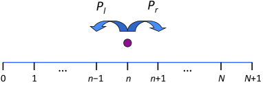
Figure 1: An illustration of a one-dimensional single random walk.

Now consider $M$ random walks on the same network, where the particle in each random walk behaves independently identically as in the single random walk described above. Let $B_{i}(k,n)$ be the Bernoulli random variable representing the presence of the $i$th particle at point $n$ at time instant $k$, where $k=0,1,\ldots$ and $n=1,\ldots,N$. Define $B_{i}(k)=[B_{i}(k,1),\ldots,B_{i}(k,N)]^{T}\in{\mathbb{R}}^{N}$. According to the behavior of the particle in the single random walk, for $i=1,\ldots,M$,

$$B_{i}(k+1,n)-B_{i}(k,n)$$

$$=\left\{\begin{array}[]{lr}B_{i}(k,n-1),&\mbox{ with probability }P_{r}(n-1);\\ B_{i}(k,n+1),&\mbox{ with probability }P_{l}(n+1);\\ -B_{i}(k,n),&\mbox{ with probability }P_{r}(n)+P_{l}(n);\\ 0,&\mbox{ otherwise},\\ \end{array}\right.$$

where $B_{i}(k,n)$ with $n\leq 0$ or $n\geq N+1$ are defined to be zero. Let the function $F_{N}(x,U(k))$, where $U(k)$ are i.i.d. and do not depend on $x$, be such that for $i=1,\ldots,M$,

$$B_{i}(k+1)=B_{i}(k)+F_{N}(B_{i}(k),U(k)).$$ (1)

Then for $x=[x_{1},\ldots,x_{N}]^{T}$, the $n$th component of $F_{N}(x,U(k))$, where $n=1,\ldots,N$, is

$$\left\{\begin{array}[]{lr}x_{n-1},&\mbox{ with probability }P_{r}(n-1);\\ x_{n+1},&\mbox{ with probability }P_{l}(n+1);\\ -x_{n},&\mbox{ with probability }P_{r}(n)+P_{l}(n);\\ 0,&\mbox{ otherwise},\end{array}\right.$$ (6)

where $x_{n}$ with $n\leq 0$ or $n\geq N+1$ are defined to be zero.

Let $X_{N}(k,n)$ be the number of particles at point $n$ at time $k$. Then

$$X_{N}(k,n)=\sum_{i=1}^{M}B_{i}(k,n).$$ (7)

Define $X_{N}(k)=[X_{N}(k,1),\ldots,X_{N}(k,N)]^{T}$, which forms a discrete-time Markov chain with state space ${\mathbb{R}}^{N}$. Since $F_{N}$ is linear, it follows from (7) that

$$X_{N}(k+1)=X_{N}(k)+F_{N}(X_{N}(k),U(k)).$$

Let

$$f_{N}(x)=EF_{N}(x,U(k)),\quad x\in{\mathbb{R}}^{N}.$$

It follows from (6) that for $x=[x_{1},\ldots,x_{N}]^{T}$, the $n$th component of $f_{N}(x)$, where $n=1,\ldots,N$, is

$$P_{r}(n-1)x_{n-1}+P_{l}(n+1)x_{n+1}-(P_{r}(n)+P_{l}(n))x_{n},$$ (8)

where $x_{n}$ with $n\leq 0$ or $n\geq N+1$ are defined to be zero. By (1) and the linearity of $F_{N}$, for $i=1,\ldots,M$,

$$EB_{i}(k+1)=EB_{i}(k)+f_{N}(EB_{i}(k)).$$ (9)

Notice that, since the random walks are i.i.d., $EB_{i}$ does not depend on $i$. Define a deterministic sequence $x_{N}(k)$ by

$$x_{N}(k+1)=x_{N}(k)+f_{N}(x_{N}(k)),$$ (10)

where

$$x_{N}(0)=\frac{X_{N}(0)}{M},\mbox{ a.s.\ (almost surely).}$$ (11)

We seek to approximate $X_{N}(k)$ by a continuum model, where the time and space indices $k$ and $n$ are made continuous as $N\rightarrow\infty$ and $M\rightarrow\infty$ in the following two steps: First, define

$$X_{oN}(\tilde{t})=\frac{X_{N}(\lfloor M\tilde{t}\rfloor)}{M},$$

the continuous-time extension of $X_{N}(k)$ by piecewise-constant time extensions with interval length $dt=1/M$ and scaled by $1/M$. Second, define $X_{pN}(t,s)$ to be the continuous-space extension of $X_{oN}(\tilde{t})$ by piecewise-constant space extensions on $\mathcal{D}$ with interval length $ds$. Notice that as $N\rightarrow\infty$, $ds\rightarrow 0$. Thus $X_{pN}$ is the continuous-time-space extension of $X_{N}(k)$. Similarly, define $x_{oN}(\tilde{t})=x_{N}(\lfloor M\tilde{t}\rfloor)$, the piecewise-constant continuous-time extension of $x_{N}(k)$, and $x_{pN}(t,s)$, the piecewise-constant continuous-space extension of $x_{oN}(\tilde{t})$. Thus $x_{pN}$ is the continuous-time-space extension of $x_{N}(k)$.

Now we show that for $M$ sufficiently large, $X_{pN}$, the continuous-time-space extension of $X_{N}(k)$, is close to $x_{pN}$, the continuous-time-space extension of $x_{N}(k)$. By (7) and the strong law of large numbers (SLLN), for each $k$,

$$\lim_{M\rightarrow\infty}\frac{X_{N}(k)}{M}=EB_{i}(k)\mbox{ a.s.}$$

By this and (11),

$$\lim_{M\rightarrow\infty}x_{N}(0)=EB_{i}(0)\mbox{ a.s.}$$

By (9) and (10), $x_{N}(k)$ and $EB_{i}(k)$ satisfy the same difference equation. Then we have for each $k$,

$$\lim_{M\rightarrow\infty}x_{N}(k)=EB_{i}(k)\mbox{ a.s.}$$

Hence for each $k$,

$$\lim_{M\rightarrow\infty}\frac{X_{N}(k)}{M}=x_{N}(k)\mbox{ a.s.}$$

Therefore, $X_{oN}$ and $x_{oN}$ are close for large $M$ in the sense that

$$\lim_{M\rightarrow\infty}\|X_{oN}(\tilde{t})-x_{oN}(\tilde{t})\|_{\infty}^{(N)}=0\mbox{ a.s.},$$ (12)

where $\|\cdot\|_{\infty}^{(N)}$ is the $\infty$-norm on ${\mathbb{R}}^{N}$. Note that

$$\|X_{pN}(\cdot,t)-x_{pN}(\cdot,t)\|_{\infty}^{(\mathcal{D})}=\|X_{oN}-x_{oN}\|_{\infty}^{(N)},$$

where $\|\cdot\|_{\infty}^{(\mathcal{D})}$ is the $\infty$-norm on ${\mathbb{R}}^{\mathcal{D}}$, the space of functions of $\mathcal{D}\to{\mathbb{R}}$. Then by (12), $X_{pN}$ and $x_{pN}$ are close to each other for large $M$ in the sense that

$$\lim_{M\rightarrow\infty}\|X_{pN}(\cdot,t)-x_{pN}(\cdot,t)\|_{\infty}^{(\mathcal{D})}=0\mbox{ a.s.}$$ (13)

Therefore, we can approximate $X_{pN}$ by $x_{pN}$ for $M$ sufficiently large.

Next we show that as $N\rightarrow\infty$, $x_{pN}$ satisfies a certain PDE that is easily solvable. By (8) we have for $n=1,\ldots,N$,

$$x_{N}(k+1,n)-x_{N}(k,n)$$

$$=P_{r}(n-1)x_{N}(k,n-1)+P_{l}(n+1)x_{N}(k,n+1)$$

$$\quad-(P_{r}(n)+P_{l}(n))x_{N}(k,n),$$

where $x_{N}(k,n)$ with $n\leq 0$ or $n\geq N+1$ are defined to be zero. Assume $P_{l}(n)=p_{l}(nds)$ and $P_{r}(n)=p_{r}(nds)$, where $p_{l}(s)$ and $p_{r}(s)$ are real-valued functions defined on $\mathcal{D}$. Then by the definition of $x_{pN}$, it follows that for $s\in\mathcal{D}$ and $t>0$,

$$x_{pN}(t+dt,s)-x_{pN}(t,s)$$

$$=p_{r}(s-ds)x_{pN}(t,s-ds)+p_{l}(s+ds)x_{pN}(t,s+ds)$$

$$\quad-(p_{r}(s)+p_{l}(s))x_{pN}(t,s).$$ (14)

To ensure a finite non-degenerate limit, we assume

$$p_{l}(s)=b(s)+c_{l}(s)ds\mbox{ and }p_{r}(s)=b(s)+c_{r}(s)ds.$$

Define $c=c_{l}-c_{r}.$ We call $b$ the diffusion coefficient and $c$ the convection coefficient, for a greater $b$ means more rapid diffusion and a greater $c$ means a larger directional bias. Assume that $b\in\mathcal{C}^{2}$ and $c\in\mathcal{C}^{1}$. Assume that $x_{pN}$ is twice continuously differentiable in $s$. Put into (14) the Taylor expansions

$$x_{pN}(t,s\pm ds) =x_{pN}(t,s)\pm\frac{\partial x_{pN}}{\partial s}(t,s)ds$$

$$\quad+\frac{\partial^{2}x_{pN}}{\partial s^{2}}(t,s)\frac{ds^{2}}{2}+o(ds^{2}),$$ (15)

$$b(s\pm ds)=b(s)\pm b_{s}(s)ds+b_{ss}(s)\frac{ds^{2}}{2}+o(ds^{2}),$$ (16)

and

$$c(s\pm ds)=c(s)\pm c_{s}(s)ds+o(ds),$$ (17)

where a single subscript $s$ represents first derivative and a double subscript $ss$ represents second derivative. Then we have

$$x_{pN}(t+dt,s)-x_{pN}(t,s)=b(s)\frac{\partial^{2}x_{pN}}{\partial s^{2}}(t,s)ds^{2}$$

$${}+(2b_{s}(s)+c(s))\frac{\partial x_{pN}}{\partial s}(t,s)ds^{2}$$

$${}+(b_{ss}(s)+c_{s}(s))x_{pN}(t,s)ds^{2}+o(ds^{2}).$$ (18)

Divide both sides of (18) by $dt=ds^{2}$ and get

$$\frac{x_{pN}(t+dt,s)-x_{pN}(t,s)}{dt}$$

$$=b(s)\frac{\partial^{2}x_{pN}}{\partial s^{2}}(t,s)+(2b_{s}(s)+c(s))\frac{\partial x_{pN}}{\partial s}(t,s)$$

$$\quad+(b_{ss}(s)+c_{s}(s))x_{pN}(t,s)+\frac{o(ds^{2})}{ds^{2}}.$$

As $N\rightarrow\infty$, $ds\rightarrow 0$, and hence $dt=ds^{2}\rightarrow 0.$ Assume that $x_{pN}$ is continuously differentiable in $t$. Then by taking the limit as $N\rightarrow\infty$ and rearranging, we get a PDE that $x_{pN}$ satisfies:

$$\dot{x}_{pN}(t,s) =\frac{\partial}{\partial s}\left(b(s)\frac{\partial x_{pN}}{\partial s}(t,s)\right)$$

$$\quad+\frac{\partial}{\partial s}((b_{s}(s)+c(s))x_{pN}(t,s)),$$

for $t>0$ and $s\in\mathcal{D}$, with boundary condition $x_{pN}(t,s)=0$.

As $N\rightarrow\infty$, $dt=ds^{2}\rightarrow 0$, and hence $M=1/dt=1/ds^{2}\rightarrow\infty$. Then by (13), for $N$ sufficiently large, $X_{pN}$, the continuous-time-space extension of $X_{N}(k)$, is close to $x_{pN}$, the continuous-time-space extension of $x_{N}(k)$. Therefore, we can approximate $X_{N}(k)$ by the solution of the above PDE called the one-dimensional diffusion-convection equation, which can be easily solved [25]. Note that our derivation here differs from that of the well-studied Fokker-Planck equation (also known as the Kolmogorov forward equation) [26], whereas the latter originates from the study of the probability density of a Wiener process.

This motivational example raises some questions that must be answered by the convergence analysis of the underlying limiting process. First, general networks may exhibit more complex behaviors. For example, $F_{N}$ might no longer be linear; and SLLN might not apply in many scenarios since node behaviors are not necessarily i.i.d. Specifically, the analysis above does not apply to the network Markov chain in [7]. To find the conditions under which (12) holds in more general setting, in Section III-B we apply Kushner’s weak convergence theorem in [4] to a more general class of systems modeled by Markov chains. Moreover, we need to show in what sense and under what conditions $X_{pN}$ converges to the solution of the PDE. We analyze such convergence and provide its sufficient conditions in Section III-C.

III Continuum Limits of Markov Chains

In this section we analyze the convergence of a sequence of Markov chains to the solution of a PDE in a two-step procedure. We provide sufficient conditions for this convergence.

III-A General Setting

Consider $N$ points placed over a Euclidean domain $\mathcal{D}$ representing a spatial region. We assume that these points form a uniform grid, though our approach can later be generalized to nonuniform cases. We will refer to these $N$ points in $\mathcal{D}$ as grid points and denote the distance between any two neighboring grid points by $ds_{N}$.

Consider a discrete-time Markov chain

$$X_{N}(k)=[X_{N}(k,1),\ldots,X_{N}(k,N)]^{T}$$ (19)

with state space ${\mathbb{R}}^{N}$. Here $X_{N}(k,n)$ is the real-valued state of point $n$ at time $k$, where $n=1,\ldots,N$ is a spatial index and $k=0,1,\ldots$ is a temporal index.

Suppose that the evolution of $X_{N}(k)$ is described by the stochastic difference equation

$$X_{N}(k+1)=X_{N}(k)+F_{N}(X_{N}(k)/M,U(k)),$$ (20)

where $U(k)$ are i.i.d. and do not depend on the state $X_{N}(k)$, $M$ is a “normalizing” parameter, and $F_{N}$ is a given function. Let

$$f_{N}(x)=EF_{N}(x,U(k)),\quad x\in{\mathbb{R}}^{N}.$$ (21)

Define a deterministic sequence $x_{N}(k)$ by

$$x_{N}(k+1)=x_{N}(k)+\frac{1}{M}f_{N}(x_{N}(k)),$$ (22)

where $x_{N}(0)=X_{N}(0)/M$ a.s. In the next subsection, we show that under certain conditions, $X_{N}(k)/M$ and $x_{N}(k)$ are close in some sense.

III-B Convergence to ODE

Let $X_{oN}(\tilde{t})$ be the continuous-time extension of $X_{N}(k)$ by piecewise-constant time extensions with interval length $1/M$ and scaled by $1/M$, i.e., for arbitrary $\tilde{t}\in{\mathbb{R}}$,

$$X_{oN}(\tilde{t})=X_{N}(\lfloor M\tilde{t}\rfloor)/M.$$ (23)

It follows that for each $k$, $X_{oN}(k/M)=X_{N}(k)/M$. Similarly we define $x_{oN}(\tilde{t})$, the continuous-time extension of $x_{N}(k)$ by

$$x_{oN}(\tilde{t})=x_{N}(\lfloor M\tilde{t}\rfloor).$$ (24)

For fixed $\tilde{T}_{N}>0$, let $D^{N}[0,\tilde{T}_{N}]$ be the space of ${\mathbb{R}}^{N}$-valued Càdlàg functions on $[0,\tilde{T}_{N}]$, i.e., functions that are right-continuous at each $t\in[0,\tilde{T}_{N})$ and have left-hand limits at each $t\in(0,\tilde{T}_{N}]$. As defined in (23) and (24) respectively, both $X_{oN}(\tilde{t})$ and $x_{oN}(\tilde{t})$ with $\tilde{t}\in[0,\tilde{T}_{N}]$ are in $D^{N}[0,\tilde{T}_{N}].$ Since both $X_{oN}(\tilde{t})$ and $x_{oN}(\tilde{t})$ depend on $M$, each one of them forms a sequence of functions in $D^{N}[0,\tilde{T}_{N}]$ indexed by $M=1,2,\ldots$.

Define the $\infty$-norm $\|\cdot\|_{\infty}^{(o)}$ on $D^{N}[0,\tilde{T}_{N}]$, i.e., for $x\in D^{N}[0,\tilde{T}_{N}]$,

$$\|x\|_{\infty}^{(o)}=\max_{n=1,\ldots,N}\sup_{t\in[0,\tilde{T}_{N}]}|x^{n}(t)|,$$

where $x^{n}$ is the $n$th components of $x$. A sequence of functions $x_{M}\in D^{N}[0,\tilde{T}_{N}]$ is said to converge uniformly to a function $x\in D^{N}[0,\tilde{T}_{N}]$ if as $M\rightarrow\infty$, $\|x_{M}-x\|_{\infty}^{(o)}\to 0$. In this paper, we use the notation “$\Rightarrow$” for weak convergence and “$\xrightarrow{P}$” for convergence in probability.

Let $f_{N}$ be defined as in (21). Now we present a lemma stating that under some conditions, as $M\rightarrow\infty$, $X_{oN}$ converges uniformly to a limiting function $y$, the solution of the ODE $\dot{y}=f_{N}(y)$, on $[0,\tilde{T}_{N}]$, and $X_{oN}$ converges uniformly to the same solution on $[0,\tilde{T}_{N}]$.

Lemma 1

Assume:

1. There exists an identically distributed sequence $\{\lambda(k)\}$ of integrable random variables such that for each $k$ and $x$, $|F_{N}(x,U(k))|\leq\lambda(k)$ a.s.;

2. the function $F_{N}(x,U(k))$ is continuous in $x$ a.s.; and

3. the ODE $\dot{y}=f_{N}(y)$ has a unique solution on $[0,\tilde{T}_{N}]$ for any initial condition $y(0)$.

Suppose that as $M\to\infty$,

$$X_{oN}(0)\xrightarrow{P}y(0)\mbox{ and }x_{oN}(0)\to y(0).$$

Then, as $M\to\infty$,

$$\|X_{oN}-y\|_{\infty}^{(o)}\xrightarrow{P}0\mbox{ and }\|x_{oN}-y\|_{\infty}^{(o)}\to 0$$

on $[0,\tilde{T}_{N}]$, where $y$ is the unique solution of $\dot{y}=f_{N}(y)$ with initial condition $y(0)$.

To prove Lemma 1, we first present a lemma on weak convergence due to Kushner [4].

Lemma 2

Assume:

1. The set

   $$\{|F_{N}(x,U(k))|:k\geq 0\}$$

   is uniformly integrable;

2. for each $k$ and each bounded random variable $X$,

   $$\lim_{\delta\rightarrow 0}E\sup_{|Y|\leq\delta}|F_{N}(X,U(k))-F_{N}(X+Y,U(k))|=0;$$

   and

3. there is a function $\hat{f}_{N}(\cdot)$ [continuous by (b)] such that as $n\rightarrow\infty$,

   $$\frac{1}{n}\sum^{n}_{k=0}{F_{N}(x,U(k))\xrightarrow{P}\hat{f}_{N}(x)}.$$

Suppose that $\dot{y}=\hat{f}_{N}(y)$ has a unique solution on $[0,\tilde{T}_{N}]$ for each initial condition, and that $X_{oN}(0)\Rightarrow y(0)$. Then as $M\to\infty$,

$$\|X_{oN}-y\|_{\infty}^{(o)}\Rightarrow 0\mbox{ on }[0,\tilde{T}_{N}].$$

We note that in Kushner’s work, the convergence of $X_{oN}$ to $y$ is stated in terms of Skorokhod norm [4], but it is equivalent to the $\infty$-norm in our case where the functions are defined on finite time intervals [27].

We now prove Lemma 1 by showing that the assumptions (2a)–(2c) in Lemma 2 hold under the assumptions (1a)–(1c) in Lemma 1.

• Proof of Lemma 1:

  1. Since $\lambda(k)$ is integrable, as $a\rightarrow\infty$,

     $$E|\lambda(k)|1_{\{|\lambda(k)|>a\}}\rightarrow 0,$$

     where $1_{A}$ is the indicator function of set $A$. By Assumption (1a), for each $k$ and $x$,

     $$F_{N}(x,U(k))\leq\lambda(k)\mbox{ a.s.}$$

     Therefore for each $x$ and $a>0$,

     $$E|F_{N}(x,U(k))|1_{\{|F_{N}(x,U(k))|>a\}}$$

     $$\leq E|\lambda(k)|1_{\{|F_{N}(x,U(k))|>a\}}$$

     $$\leq E|\lambda(k)|1_{\{|\lambda(k)|>a\}}.$$

     Hence as $a\rightarrow\infty$,

     $$\sup_{k\geq 0}E|F_{N}(x,U(k))|1_{\{|F_{N}(x,U(k))|>a\}}\rightarrow 0,$$

     i.e., the family $\{|F_{N}(x,U(k))|:k\geq 0\}$ is uniformly integrable and Assumption (2a) holds.

  2. By Assumption (1b), $F_{N}(x,U(k))$ is continuous in $x$ a.s. Then for each bounded $X$ and each $k$,

     $$\lim_{\delta\rightarrow 0}\sup_{|Y|\leq\delta}|F_{N}(X,U(k))-F_{N}(X+Y,U(k))|=0\mbox{ a.s.}$$

     By Assumption (1a), for each $x$ and each $k$, there exists an integrable random variable $\lambda(k)$ such that $|F_{N}(x,U(k))|\leq\lambda(k)$ a.s. It follows that for each bounded $X$, each $k$, and each $Y$ such that $|Y|\leq\delta$,

     $$|F_{N}(X,U(k))-F_{N}(X+Y,U(k))|$$

     $$\leq|F_{N}(X,U(k))|+|F_{N}(X+Y,U(k))|\leq 2\lambda(k).$$

     Hence for each $\delta$,

     $$\left|\sup_{|Y|\leq\delta}|F_{N}(X,U(k))-F_{N}(X+Y,U(k))|\right|\leq 2\lambda(k),$$

     an integrable random variable. By the dominant convergence theorem,

     $$\lim_{\delta\rightarrow 0}E\sup_{|Y|\leq\delta}|F_{N}(X,U(k))-F_{N}(X+Y,U(k))|$$

     $$=E\lim_{\delta\rightarrow 0}\sup_{|Y|\leq\delta}|F_{N}(X,U(k))-F_{N}(X+Y,U(k))|$$

     $$=0.$$

     Hence Assumption (2b) holds.

  3. Since $U(k)$ are i.i.d., by the weak law of large numbers and the definition of $f_{N}$ in (21), as $n\rightarrow\infty$,

     $$\frac{1}{n}\sum^{n}_{k=0}{F_{N}(x,U(k))\xrightarrow{P}f_{N}(x)}.$$

     Hence Assumption (2c) holds.

  Then, by Lemma 2, as $M\to\infty$, $\|X_{oN}-y\|_{\infty}^{(o)}\Rightarrow 0$ on $[0,\tilde{T}_{N}]$. For each sequence of random processes $\{X_{n}\}$, if $A$ is a constant, $X_{n}\Rightarrow A$ if and only if $X_{n}\xrightarrow{P}A$. Therefore, as $M\to\infty$, $\|X_{oN}-y\|_{\infty}^{(o)}$$\xrightarrow{P}0$ on $[0,\tilde{T}_{N}]$. The same argument implies the deterministic convergence of $x_{oN}$: as $M\rightarrow\infty$, $\|x_{oN}-y\|_{\infty}^{(o)}\to 0$ on $[0,\tilde{T}_{N}]$.  

Based on Lemma 1, we get the following lemma, which states that $X_{oN}$ and $x_{oN}$ are close with high probability when $M$ is large.

Lemma 3

Let the assumptions in Lemma 1 hold. Then for any sequence $\{\zeta_{N}\}$, for each $N$, and for $M$ sufficiently large, we have

$$P\{\|X_{oN}-x_{oN}\|_{\infty}^{(o)}>\zeta_{N}\}\leq 1/N^{2}\mbox{ on }[0,\tilde{T}_{N}].$$

Proof:

By Lemma 1, for each $N$, as $M\to\infty$,

$$\|X_{oN}-y\|_{\infty}^{(o)}\xrightarrow{P}0\mbox{ and }\|x_{oN}-y\|_{\infty}^{(o)}\to 0\mbox{ on }[0,\tilde{T}_{N}].$$

By the triangle inequality

$$\|X_{oN}-x_{oN}\|_{\infty}^{(o)}\leq\|X_{oN}-y\|_{\infty}^{(o)}+\|x_{oN}-y\|_{\infty}^{(o)},$$

it follows that as $M\to\infty$, $\|X_{oN}-x_{oN}\|_{\infty}^{(o)}\xrightarrow{P}0$ on $[0,\tilde{T}_{N}]$. This finishes the proof. ∎

Since $X_{oN}$ and $x_{oN}$ are the piecewise continuous-time extensions of $X_{N}$ and $x_{N}$ by constant interpolation, respectively, we have the following corollary.

Corollary 1

Fix $\tilde{T}_{N}$ and let $\tilde{K}_{N}=\lfloor\tilde{T}_{N}M\rfloor$. Let the assumptions in Lemma 1 hold. Then for any sequence $\{\zeta_{N}\}$, for each $N$, and for $M$ sufficiently large, we have

$$P\left\{\max_{{k=0,\ldots,\tilde{K}_{N}}\atop{n=1,\ldots,N}}\left|\frac{X_{N}(k,n)}{M}-x_{N}(k,n)\right|>\zeta_{N}\right\}\leq\frac{1}{N^{2}}.$$

We use Lemma 3 and Corollary 1 in the next subsection.

III-C Convergence to PDE

In the last subsection, we stated conditions under which the continuous-time extensions of $X_{N}(k)$ and $x_{N}(k)$ are close asymptotically (as $M\to\infty$) with high probability. In this subsection, we further let $N\to\infty$ and state conditions under which $x_{N}(k)$ is close asymptotically to the solution of a PDE. This leads to the convergence of $X_{N}(k)/M$ to the PDE solution as $M\to\infty$ and $N\to\infty$.

Assume that the domain $\mathcal{D}$ introduced in Section III-A is compact and convex, and let $w:\mathcal{D}\to{\mathbb{R}}$ be in $\mathcal{C}^{2}$. Given a fixed $N$, let $V_{N}$ be the set of the $N$ grid points in $\mathcal{D}$. Let $y_{N}$ be the vector in ${\mathbb{R}}^{N}$ composed of the values of $w$ at the grid points $v_{N}(n)\in V_{N}$, $n=1,\ldots,N$, i.e., $y_{N}=[w(v_{N}(1)),\ldots,w(v_{N}(N))]^{T}.$

Given $s\in\mathcal{D}$, let $\{s_{N}\}\subset\mathcal{D}$ be a sequence of grid points in $\mathcal{D}$ such that as $N\rightarrow\infty$, $s_{N}\rightarrow s$, where for each $N$, $s_{N}$ is a grid point in $V_{N}$. Let $f_{N}(y_{N},s_{N})$ be the component of the vector $f_{N}(y_{N})$ corresponding to the location $s_{N}$. For example, for $N=5$, if $s_{5}=v_{5}(4)$ in $V_{5}$, then $f_{5}(y_{5},s_{5})$ is the 4th component of the vector $f_{5}(y_{5})$.

Assume that there exist sequences $\{\delta_{N}\}$, $\{\beta_{N}\}$, $\{\gamma_{N}\}$, and $\{\rho_{N}\}$, functions $f$ and $h$, and $0<c<\infty$, such that as $N\rightarrow\infty,\delta_{N}\rightarrow 0,\delta_{N}/\beta_{N}\rightarrow 0,\gamma_{N}\to 0,\rho_{N}\to 0$, and:

• for any $s_{N}$ such that $s_{N}\to s$, where $s$ is in the interior of $\mathcal{D}$, there exists a sequence of functions $\phi_{N}:\mathcal{D}\to{\mathbb{R}}$ such that

  $$f_{N}(y_{N},s_{N})/\delta_{N} =f(s_{N},w(s_{N}),\nabla w(s_{N}),\nabla^{2}w(s_{N}))$$

  $$\quad+\phi_{N}(s_{N}),$$ (25)

  and for $N$ sufficiently large,

  $$|\phi_{N}(s_{N})|\leq c\gamma_{N};$$ (26)

  and

• for any $s_{N}$ such that $s_{N}\to s$, where $s$ is on the boundary of $\mathcal{D}$, there exists a sequence of functions $\varphi_{N}:\mathcal{D}\to{\mathbb{R}}$ such that

  $$f_{N}(y_{N},s_{N})/\beta_{N} =h(s_{N},w(s_{N}),\nabla w(s_{N}),\nabla^{2}w(s_{N}))$$

  $$\quad+\varphi_{N}(s_{N}),$$ (27)

  and for $N$ sufficiently large, $|\varphi_{N}(s_{N})|\leq c\rho_{N}$.

Here, $\nabla^{i}w$ represents all the $i$th order derivatives of $w$, where $i=1,2$.

These assumptions are technical conditions on the asymptotic behavior of the sequence of functions $f_{N}$. The basic idea is that $f_{N}(y_{N},s_{N})$ is asymptotically close to some function of terms that look like the right-hand side of a time-dependent PDE. Typically, checking these conditions amounts to simply an algebraic exercise. A concrete example of this is given in the next section.

The basic idea underlying the analysis in the remainder of this subsection is this. Recall that $x_{N}(k)$ is defined by (22). Suppose we associate the discrete time $k$ with points on the real line spaced apart by a distance proportional to $\delta_{N}$. Then, the above technical assumption implies that $x_{N}(k)$ is, in some sense, close to the solution of a PDE of the form $\dot{z}=f(s,z,\nabla z,\nabla^{2}z)$ with boundary condition $h(s,z,\nabla z,\nabla^{2}z)=0$. Because the Markov chain $X_{N}(k)/M$ is close to $x_{N}(k)$, as established in the last subsection, it is also close to the solution of the PDE. The remainder of this subsection is devoted to developing this argument rigorously.

Fix $T>0$. Assume that there exists a function $z:[0,T]\times\mathcal{D}\to{\mathbb{R}}$ that solves the PDE

$$\dot{z}(t,s)=f(s,z(t,s),\nabla z(t,s),\nabla^{2}z(t,s)),$$ (28)

with boundary condition

$$\ h(s,z(t,s),\nabla z(t,s)\nabla^{2}z(t,s))=0$$

and initial condition $z(0,s)=z_{0}(s)$. Here, $\nabla^{i}z(t,s)$ represents all the $i$th order partial derivatives of $z(t,s)$ with respect to $s$, where $i=1,2$.

Define

$$dt_{N}=\delta_{N}/M.$$ (29)

Define

$$K_{N}=\lfloor T/dt_{N}\rfloor\mbox{ and }t_{N}(k)=kdt_{N}.$$

Define

$$z_{N}(k,n)=z(t_{N}(k),v_{N}(n))$$

and let $z_{N}(k)=[z_{N}(k,1),\ldots,z_{N}(k,N)]^{T}\in{\mathbb{R}}^{N}$.

Denote the $\infty$-norm on ${\mathbb{R}}^{N}$ by $\|\cdot\|^{(N)}_{\infty}$. That is, for $x\in{\mathbb{R}}^{N}$, with the $n$th element being $x(n)$,

$$\|x\|^{(N)}_{\infty}=\max_{1\leq n\leq N}|x(n)|.$$

Denote the $\infty$-norm on ${\mathbb{R}}^{N\times K_{N}}$ also by $\|\cdot\|^{(N)}_{\infty}$. That is, for $x=[x(1),\ldots,x(K_{N})]\in{\mathbb{R}}^{N\times K_{N}}$, where for $k=1,\ldots,K_{N}$, $x(k)=[x(k,1),\ldots,x(k,N)]^{T}\in{\mathbb{R}}^{N}$, we have

$$\|x\|_{\infty}^{(N)}=\max_{{k=1,\ldots,K_{N}}\atop{n=1,\ldots,N}}|x(k,n)|.$$

Now we present a lemma on the relationship between the $z_{N}(k)$ and $f_{N}$.

Lemma 4

Assume that $z$ is continuously differentiable in $t$. Then for each $N$, there exists $u_{N}(k)\in{\mathbb{R}}^{N}$ such that for $k=0,\ldots,K_{N}-1$,

$$z_{N}(k+1)-z_{N}(k)=\frac{1}{M}f_{N}(z_{N}(k))+dt_{N}u_{N}(k),$$ (30)

and

$$\|u_{N}\|^{(N)}_{\infty}=O(\max\{\gamma_{N},dt_{N}\}),$$ (31)

where $u_{N}=[u_{N}(0),\ldots,u_{N}(K_{N}-1)]\in{\mathbb{R}}^{N\times K_{N}}.$

Proof:

Since $z$ is continuously differentiable in $t$, there exists $0<c_{1}<\infty$ such that for each $N$, for $k=0,\ldots,K_{N}-1$ and $n=1,\ldots,N$, there exists a function $r_{N}:[0,T]\times\mathcal{D}\to{\mathbb{R}}$ such that

$$\frac{z_{N}(k+1,n)-z_{N}(k,n)}{dt_{N}}$$

$$=\frac{z(t_{N}(k),v_{N}(n))-z(t_{N}(k),v_{N}(n))}{dt_{N}}$$

$$=\dot{z}(t_{N}(k),v_{N}(n))+r_{N}(t_{N}(k),v_{N}(n)),$$ (32)

and for $N$ sufficiently large, $|r_{N}(t_{N}(k),v_{N}(n))|<c_{1}dt_{N}$.

By (25) and (28), there exists $0<c_{2}<\infty$, such that for each $N$, for $k=0,\ldots,K_{N}-1$ and $n=1,\ldots,N$, there exists a function $\phi_{N}:[0,T]\times\mathcal{D}\to{\mathbb{R}}$ such that

$$\dot{z}(t_{N}(k),v_{N}(n))$$

$$=f(v_{N}(n),z_{N}(k,n),\nabla z_{N}(k,n),\nabla^{2}z_{N}(k,n))$$

$$=f_{N}(z_{N}(k),v_{N}(n))/\delta_{N}+\phi_{N}(t_{N}(k),v_{N}(n)),$$ (33)

and for $N$ sufficiently large, $|\phi_{N}(t_{N}(k),v_{N}(n))|<c_{2}\gamma_{N}$, where $\{\gamma_{N}\}$ is as defined in (26).

For each $N$, for $k=0,\ldots,K_{N}-1$ and $n=1,\ldots,N$, let

$$u_{N}(k,n)=\phi_{N}(t_{N}(k),v_{N}(n))+r_{N}(t_{N}(k),v_{N}(n)),$$

and $u_{N}(k)=[u_{N}(k,1),\ldots,u_{N}(k,N)]^{T}\in{\mathbb{R}}^{N}$. Then there exists $0<c<\infty$ such that for each $N$,

$$\|u_{N}\|^{(N)}_{\infty}<c\max\{\gamma_{N},dt_{N}\}.$$

Hence (31) follows.

By (32) and (33), for each $N$, for $k=0,\ldots,K_{N}-1$ and $n=1,\ldots,N$,

$$\frac{z_{N}(k+1)-z_{N}(k)}{dt_{N}}=\frac{f_{N}(z_{N}(k))}{\delta_{N}}+u_{N}(k).$$

By this and (29), we have (30). ∎

In the following we show that under some conditions, $x_{N}(k)$ and $z_{N}(k)$ are asymptotically close for large $N$.

For each $N$, for $k=0,\ldots,K_{N}$ and $n=1,\ldots,N$, define

$$\varepsilon_{N}(k,n)=z_{N}(k,n)-x_{N}(k,n),$$ (34)

and let $\varepsilon_{N}(k)=[\varepsilon_{N}(k,1),\ldots,\varepsilon_{N}(k,N)]^{T}\in{\mathbb{R}}^{N}$.

By (22), (30), and (34), we have that for each $N$, for $k=0,\ldots,K_{N}$, there exists $u_{N}(k)$ as defined in Lemma 4 such that

$$\varepsilon_{N}(k+1) =\varepsilon_{N}(k)+\frac{1}{M}(f_{N}(z_{N}(k))-f_{N}(x_{N}(k)))$$

$$\quad+dt_{N}u_{N}(k).$$ (35)

Suppose that for each $N$, $f_{N}\in\mathcal{C}^{1}$. Let $Df_{N}(x)$ be the derivative matrix of the function $f_{N}$ at $x$. Then we have that for each $N$, for $k=1,\ldots,K_{N}$ and $n=1,\ldots,N$, there exists a function $\tilde{f}_{N}:{\mathbb{R}}^{N}\to{\mathbb{R}}^{N}$ such that

$$f_{N}(z_{N}(k))-f_{N}(x_{N}(k))=Df_{N}(z_{N}(k))\varepsilon_{N}(k)+\tilde{f}_{N}(\varepsilon_{N}(k))$$

and

$$\tilde{f}_{N}(0)=0.$$ (36)

Then we have from (35)

$$\varepsilon_{N}(k+1) =\varepsilon_{N}(k)+\frac{1}{M}(Df_{N}(z_{N}(k))\varepsilon_{N}(k)$$

$$\quad+\tilde{f}_{N}(\varepsilon_{N}(k)))+dt_{N}u_{N}(k).$$ (37)

Further suppose that for each $N$,

$$\|\varepsilon_{N}(0)\|_{\infty}^{(N)}=0.$$ (38)

Define $\varepsilon_{N}=[\varepsilon_{N}(1),\ldots,\varepsilon_{N}(K_{N})]\in{\mathbb{R}}^{N\times K_{N}}$. Then by  (36), (37), and (38), for each $N$, there exists a function $H_{N}:{\mathbb{R}}^{N\times K_{N}}\to{\mathbb{R}}^{N\times K_{N}}$ such that

$$\varepsilon_{N}=H_{N}(u_{N}).$$ (39)

It follows that $H_{N}(0)=0$ and $H_{N}\in\mathcal{C}^{1}$.

For each $N$, define

$$\mu_{N}=\lim_{\alpha\to 0}\sup_{\|u\|_{\infty}^{(N)}\leq\alpha}\frac{\|H_{N}(u)\|_{\infty}^{(N)}}{\|u\|_{\infty}^{(N)}}.$$

Lemma 5

Assume that

• $z$ is continuously differentiable in $t$;

• for each $N$, $f_{N}\in\mathcal{C}^{1}$;

• for each $N$, (38) holds; and

• the sequence $\{\mu_{N}\}$ is bounded.

Then

$$\|\varepsilon_{N}\|_{\infty}^{(N)}=O(\|u_{N}\|_{\infty}^{(N)}).$$

Proof:

By definition, for each $N$, there exists $\delta>0$ such that for $\alpha<\delta$,

$$\sup_{\|u\|_{\infty}^{(N)}\leq\alpha}\frac{\|H_{N}(u)\|_{\infty}^{(N)}}{\|u\|_{\infty}^{(N)}}<\mu_{N}+1.$$

By (31), as $N\to\infty$, $\|u\|_{\infty}^{(N)}\to 0$. Then there exists $N_{0}$ and $\alpha_{1}$ such that for $N>N_{0}$, $\|u\|_{\infty}^{(N)}\leq\alpha_{1}<\delta$. Hence, for $N>N_{0}$,

$$\frac{\|H_{N}(u)\|_{\infty}^{(N)}}{\|u\|_{\infty}^{(N)}}\leq\sup_{\|u\|_{\infty}^{(N)}\leq\alpha_{1}}\frac{\|H_{N}(u)\|_{\infty}^{(N)}}{\|u\|_{\infty}^{(N)}}<\mu_{N}+1.$$

Therefore, there exists $0<c<\infty$ such that for $N>N_{0}$,

$$\|\varepsilon_{N}\|_{\infty}^{(N)} =\|H_{N}(u_{N})\|_{\infty}^{(N)}<(\mu_{N}+1)\|u_{N}\|_{\infty}^{(N)}$$

$$<(c+1)\|u_{N}\|_{\infty}^{(N)}.$$

This finishes the proof. ∎

Lemma 5 states that as $N\to\infty$, $\|\varepsilon_{N}\|_{\infty}^{(N)}\to 0$, and at least with the same rate as $\|u_{N}\|_{\infty}^{(N)}$.

Let $X_{N}=[X_{N}(1)/M,\ldots,X_{N}(K_{N})/M]$, $x_{N}=[x_{N}(1),\ldots,x_{N}(K_{N})]$, and $z_{N}=[z_{N}(1),\ldots,z_{N}(K_{N})]$, all in $\in{\mathbb{R}}^{N\times K_{N}}$. Now we present the main convergence theorem of this paper, which states that the value of the normalized Markov chain at time $k$ and node $n$, is close to that of $z$ at the corresponding point $(t_{N}(k),v_{N}(n))\in[0,T]\times\mathcal{D}$ for large $M$ and $N$.

Theorem 1

Suppose that the assumptions in Lemma 1 and Lemma 5 hold. Then

$$\|X_{N}-z_{N}\|_{\infty}^{(N)}=O(\max\{\gamma_{N},dt_{N}\})\mbox{ a.s.}$$

Proof:

By (31) and Lemma 5, there exists $0<c_{0}<\infty$ such that for $N$ sufficiently large,

$$\|\varepsilon_{N}\|_{\infty}^{(N)}<c_{0}\max\{\gamma_{N},dt_{N}\}.$$ (40)

Let $\tilde{T}_{N}$ in Corollary 1 be $T/\delta_{N}$. Then $\tilde{K}_{N}:=\lfloor\tilde{T}_{N}M\rfloor=\lfloor T/dt_{N}\rfloor:=K_{N}$. Hence by Corollary 1, for any sequence $\{\zeta_{N}\}$, for each $N$, we can take $M$ sufficiently large such that

$$\sum_{N=1}^{\infty}P\{\|X_{N}-x_{N}\|_{\infty}^{(N)}>\zeta_{N}\}\leq\sum_{N=1}^{\infty}1/N^{2}<\infty.$$

By the first Borel-Cantelli Lemma [28],

$$P\left\{\lim\sup_{N\rightarrow\infty}\{\|X_{N}-x_{N}\|_{\infty}^{(N)}>\zeta_{N}\}\right\}=0,$$

which implies that, a.s., for $N$ sufficiently large,

$$\|X_{N}-x_{N}\|_{\infty}^{(N)}<\zeta_{N}.$$

Take $\zeta_{N}$ such that for $N$ sufficiently large,

$$\zeta_{N}<\max\{\gamma_{N},dt_{N}\}.$$

Then by the triangle inequality

$$\|X_{N}-z_{N}\|_{\infty}^{(N)} \leq\|X_{N}-x_{N}\|_{\infty}^{(N)}+\|x_{N}-z_{N}\|_{\infty}^{(N)}$$

$$=\|X_{N}-x_{N}\|_{\infty}^{(N)}+\|\varepsilon_{N}\|_{\infty}^{(N)},$$

a.s., there exists $0<c<\infty$ such that for $N$ sufficiently large,

$$\|X_{N}-z_{N}\|_{\infty}^{(N)}\leq c\max\{\gamma_{N},dt_{N}\}.$$

This finishes the proof. ∎

This theorem states that as $M\rightarrow\infty$ and $N\rightarrow\infty$, $X_{N}$ converges uniformly to $z_{N}$ a.s., and at least with the same rate as $\max\{\gamma_{N},dt_{N}\}$.

III-D Convergence of Continuous-time-space Extension

In the following we study the convergence of the continuous-time-space extension of the Markov chain $X_{N}(k)$ to the PDE solution. Set $\tilde{T}_{N}=T/\delta_{N}$. For each $N$, we can construct $X_{oN}(\tilde{t})$ and $x_{oN}(\tilde{t})$ with time interval of length $1/M$, with $\tilde{t}\in[0,\tilde{T}_{N}]$. Respectively, let $X_{pN}(t)$ and $x_{pN}(t)$, where $t\in[0,T]$, be the continuous-space extension of $X_{oN}(\tilde{t})$ and $x_{oN}(\tilde{t})$ (with $\tilde{t}\in[0,\tilde{T}_{N}]$) by piecewise-constant space extensions on $\mathcal{D}$ and with time scaled by $\delta_{N}$ so that the time-interval length is $\delta_{N}/M:=dt_{N}$. By piecewise-constant space extension of $X_{oN}$, we mean that we construct a piecewise-constant function on $\mathcal{D}$ such that the value of this function at each point in $\mathcal{D}$ is the value of the component of the vector $X_{oN}$ corresponding to the grid point that is “closest to the left” (taken one component at a time). Then for each $t$, $X_{pN}(t)$ and $x_{pN}(t)$ are real-valued functions defined on $\mathcal{D}$. Fig. 2 is an illustration of $x_{N}$ and $x_{pN}$ in a one-dimensional case.

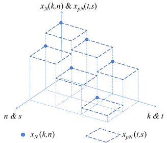
Figure 2: An illustration of $x_{N}$ and $x_{pN}$ in a one-dimensional case.

For fixed $T$, both $X_{pN}(t)$ and $x_{pN}(t)$ with $t\in[0,T]$ are in the space $D^{\mathcal{D}}[0,T]$ of functions of $[0,T]\times\mathcal{D}\to{\mathbb{R}}$ and are Càdlàg with the time component. Define the $\infty$-norm $\|\cdot\|_{\infty}^{(p)}$ on $D^{\mathcal{D}}[0,T]$, i.e., for $x\in D^{\mathcal{D}}[0,T]$,

$$\|x\|_{\infty}^{(p)}=\sup_{t\in[0,T],\atop s\in\mathcal{D}}|x(t,s)|.$$

First we show that $x_{pN}$ and $z$ are asymptotically close for large $N$.

Lemma 6

Suppose that the assumptions in Lemma 5 hold. Then

$$\|x_{pN}-z\|_{\infty}^{(p)}=O(\max\{\gamma_{N},dt_{N},ds_{N}\}).$$

Proof:

For each $N$, for $k=0,\ldots,K_{N}$ and $n=1,\ldots,N$, by the definition of $x_{pN}$, we have that $x_{pN}(t_{N}(k),v_{N}(n))=x_{N}(k,n)$. Let $\Omega_{N}(k,n)$ be the subset of $[0,T]\times\mathcal{D}$ containing $(t_{N}(k),v_{N}(n))$ where $x_{pN}$ is piecewise constant, i.e., $(t_{N}(k),v_{N}(n))\in\Omega_{N}(k,n)$ and for all $(t,s)\in\Omega_{N}(k,n)$, $x_{pN}(t,s)=x_{pN}(t_{N}(k),v_{N}(n))$. (For example, for $\mathcal{D}\subset{\mathbb{R}}$, $\Omega_{N}(k,n)=[t_{N}(k),t_{N}(k+1)]\times[v_{N}(n),v_{N}(n+1)]$.) Then for each $N$,

$$\|x_{pN}-z\|_{\infty}^{(p)}\leq\|\varepsilon_{N}\|_{\infty}^{(N)}$$

$$\quad+\max_{k=0,\ldots,K_{N}\atop n=1,\ldots,N}\sup_{(t,s)\in\Omega_{N}(k,n)}|z(t_{N}(k),v_{N}(n))-z(t,s)|.$$

Since $z(t,s)$ is continuously differentiable in $t$ on a compact domain, it is Lipschitz continuous in $t$. Similarly, it is Lipschitz continuous in $s$. Hence there exist $0<c_{1},c_{2}\leq\infty$ such that for each $N$,

$$\max_{k=0,\ldots,K_{N},\atop n=1,\ldots,N}\sup_{(t,s)\in\Omega_{N}(k,n)}|z(t_{N}(k),v_{N}(n))-z(t,s)|$$

$$\leq c_{1}\max_{k=0,\ldots,K_{N},\atop n=1,\ldots,N}\sup_{(t,s)\in\Omega_{N}(k,n)}\|(t_{N}(k),v_{N}(n))-(t,s)\|$$

$$\leq c_{2}\max\{ds_{N},dt_{N}\},$$

where $\|\cdot\|$ is some norm on $[0,T]\times\mathcal{D}$. Hence, by this and (40), there exists $0<c<\infty$ such that for $N$ sufficiently large,

$$\|x_{pN}-z\|_{\infty}^{(p)}\leq c\max\{\gamma_{N},dt_{N},ds_{N}\}.$$

This finishes the proof. ∎

Now we present a convergence theorem for the continuous functions.

Theorem 2

Suppose that the assumptions in Lemma 1 and Lemma 5 hold. Then

$$\|X_{pN}-z\|_{\infty}^{(p)}=O(\max\{\gamma_{N},dt_{N},ds_{N}\})\mbox{ a.s.\ on }[0,T]\times\mathcal{D}.$$

Proof:

By Lemma 3 , for any sequence $\{\zeta_{N}\}$, for each $N$, we can take $M$ sufficiently large such that

$$\sum_{N=1}^{\infty}P\{\|X_{oN}-x_{oN}\|_{\infty}^{(o)}>\zeta_{N}\}\leq\sum_{N=1}^{\infty}1/N^{2}<\infty.$$

By the first Borel-Cantelli Lemma [28],

$$P\left\{\lim\sup_{N\rightarrow\infty}\{\|X_{oN}-x_{oN}\|_{\infty}^{(o)}>\zeta_{N}\ \}\right\}=0,$$

which implies that, a.s., for $N$ sufficiently large,

$$\|X_{oN}-x_{oN}\|_{\infty}^{(o)}<\zeta_{N}\mbox{ on }[0,\tilde{T}_{N}].$$

Since $X_{pN}$ and $x_{pN}$ are the piecewise continuous-space extensions of $X_{oN}$ and $x_{oN}$ by constant interpolation, respectively, it follows that for any sequence $\{\zeta_{N}\}$, we can take $M$ sufficiently large such that, a.s., for $N$ sufficiently large,

$$\|X_{pN}-x_{pN}\|_{\infty}^{(p)}<\zeta_{N}\mbox{ on }[0,T]\times\mathcal{D}.$$

Take $\zeta_{N}$ such that for $N$ sufficiently large,

$$\zeta_{N}<\max\{\gamma_{N},dt_{N},ds_{N}\}.$$

Then by the triangle inequality

$$\|X_{pN}-z\|_{\infty}^{(p)}\leq\|X_{pN}-x_{pN}\|_{\infty}^{(p)}+\|x_{pN}-z\|_{\infty}^{(p)}$$

and Lemma 6, a.s., there exists $0<c<\infty$ such that for $N$ sufficiently large,

$$\|X_{pN}-z\|_{\infty}^{(p)}\leq c\max\{\gamma_{N},dt_{N},ds_{N}\}\mbox{ on }[0,T]\times\mathcal{D}.$$

This finishes the proof. ∎

This theorem states that as $M\rightarrow\infty$ and $N\rightarrow\infty$, the continuous-time-space extension $X_{pN}$ of the Markov chain $X_{N}(k)$, converges uniformly to $z$, the solution of the PDE a.s., and at least with the same rate as $\max\{\gamma_{N},dt_{N},ds_{N}\}$.

The solution of the PDE can be found quickly by mathematical tools readily available and then be used to approximate the Markov chain $X_{N}(k)$. We give an example of this in the next section.

IV Application to the Modeling of Large Networks

In this section we present an example of the application of our approach to network modeling. We show how the Markov chain representing the queue lengths of the nodes in the network can be approximated by the solution of a PDE using the results of the preceding section.

IV-A Network Model

We consider a network of wireless sensor nodes uniformly placed over a domain. In a random fashion, the sensor nodes generate data messages that need to be communicated to the destination nodes located on the boundary of the domain, which represent specialized devices that collect the sensor data. The sensor nodes also serve as relays in the routing of the messages to the destination nodes. Each sensor node has the capacity to store messages and decides to transmit or receive messages to or from its immediate neighbors at each time instant, but not both. This simplified rule of transmission allows for a relatively simple representation. We illustrate such a network over a two-dimensional domain in Fig. 3.

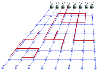
Figure 3: An illustration of a wireless sensor network over a two-dimensional domain. Destination nodes are located at the far edge. We show the possible path of a message originating from a node located in the left-front region.

The communication is interference-limited because all nodes share the same wireless channel. We assume a simple collision protocol: a transmission from a transmitter to a neighboring receiver is successful if and only if none of the other neighbors of the receiver is a transmitter, as illustrated in Fig. 4.

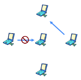
Figure 4: An illustration of the collision protocol: reception at a node fails when more than one of its neighbors transmit (regardless of the intended receiver).

$$X_{N}(k+1,n)-X_{N}(k,n)=\left\{\begin{array}[]{c}1+G(k,n),\mbox{ with probability}\\ (1-W(n,X_{N}(k,n)/M))\\ {}\times[P_{r}(n-1)W(n-1,X_{N}(k,n-1)/M)(1-W(n+1,X_{N}(k,n+1)/M))\\ {}+P_{l}(n+1)W(n+1,X_{N}(k,n+1)/M)(1-W(n-1,X_{N}(k,n-1)/M))];\\ {}-1+G(k,n),\mbox{ with probability}\\ W(n,X_{N}(k,n)/M)\\ {}\times[P_{r}(n)(1-W(n+1,X_{N}(k,n+1)/M))(1-W(n+2,X_{N}(k,n+2)/M))\\ {}+P_{l}(n)(1-W(n-1,X_{N}(k,n-1)/M))(1-W(n-2,X_{N}(k,n-2)/M))];\\ G(k,n),\mbox{ otherwise}.\end{array}\right.$$ (50)

IV-B Continuum Model in One Dimension

We first consider the case of a one-dimensional network, where $N$ sensor nodes are uniformly placed over a domain $\mathcal{D}\subset{\mathbb{R}}$ and labeled by $n=1,\ldots,N$. The destination nodes are located on the boundary of $\mathcal{D}$, labeled $n=0$ and $n=N+1$. Again let $ds_{N}$ be the distance between neighboring nodes. Let $X_{N}(k,n)$ in (19) be the queue length of node $n$ at time $k$. Let $M$ in (20) be the maximum queue length of each node.

At each time instant $k=0,1,\ldots$ , node $n$ decides to be a transmitter with probability $W(n,X_{N}(k,n)/M)$. Assume that node $n$ randomly chooses to transmit to the right or the left immediate neighbor with probability $P_{r}(n)$ and $P_{l}(n)$, respectively. Define $G(k)=[G(k,1),\ldots,G(k,N)]^{T}$, where $G(k,n)$ is the number of messages generated at node $n$ at time $k$. We model $G(k,n)$ by independent Poisson random variables with mean $g(n)$. The destination nodes at the boundaries of the domain do not have queues; they simply receive any message transmitted to it and never itself transmits anything. We illustrate the time evolution of the queues in the network in Fig. 5.

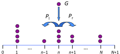
Figure 5: An illustration of the time evolution of the queues in the one-dimensional network model.

The sequence $X_{N}(k)$ defined above forms a Markov chain whose evolution is described by (20). According to the behavior of the nodes, the $n$th component of $F_{N}(X_{N}(k)/M,U(k))$, where $n=1,\ldots,N$, is defined by (50) at the top of the page, where $X_{N}(k,n)$ with $n\leq 0$ or $n\geq N+1$ are defined to be zero. For simplicity, in the following parts we set $W(n,X_{N}(k,n)/M)=X_{N}(k,n)/M$, which corresponds to the transmission rule that a node transmits a message with a probability proportional to its queue length. With this simplification, for $x=[x_{1},\ldots,x_{N}]^{T}$, the $n$th component of $F_{N}(x,U(k))$, where $n=1,\ldots,N$, is

$$\left\{\begin{array}[]{c}1+G(k,n),\mbox{ with probability}\\ (1-x_{n})[P_{r}(n-1)x_{n-1}(1-x_{n+1})\\ {}+P_{l}(n+1)x_{n+1}(1-x_{n-1})];\\ {}-1+G(k,n),\mbox{ with probability}\\ x_{n}[P_{r}(n)(1-x_{n+1})(1-x_{n+2})\\ {}+P_{l}(n)(1-x_{n-1})(1-x_{n-2})];\\ G(k,n),\mbox{ otherwise},\end{array}\right.$$

where $x_{n}$ with $n\leq 0$ or $n\geq N+1$ are defined to be zero.

Define $f_{N}$ as in (21). It follows that for $x=[x_{1},\ldots,x_{N}]^{T}$, the $n$th component of $f_{N}(x)$, where $n=1,\ldots,N$, is

$$(1-x_{n})[P_{r}(n-1)x_{n-1}(1-x_{n+1})$$

$${}+P_{l}(n+1)x_{n+1}(1-x_{n-1})]$$

$${}-x_{n}[P_{r}(n)(1-x_{n+1})(1-x_{n+2})$$

$${}+P_{l}(n)(1-x_{n-1})(1-x_{n-2})]+g(n),$$ (42)

where $x_{n}$ with $n\leq 0$ or $n\geq N+1$ are defined to be zero. Define the deterministic sequence $x_{N}(k)$ as in (22).

Set $\delta_{N}$, defined in Section III-C, to be $ds_{N}^{2}$. Let

$$dt_{N}=\delta_{N}/M=ds_{N}^{2}/M.$$ (43)

Assume

$$P_{l}(n)=p_{l}(v_{N}(n))\mbox{ and }P_{r}(n)=p_{r}(v_{N}(n)),$$ (44)

where $p_{l}(s)$ and $p_{r}(s)$ are real-valued functions defined on $\mathcal{D}$. As in Section II we again assume

$$p_{l}(s)=b(s)+c_{l}(s)ds_{N}\mbox{ and }p_{r}(s)=b(s)+c_{r}(s)ds_{N}.$$ (45)

Let $c=c_{l}-c_{r}$. Again we call $b$ the diffusion and $c$ the convection. In order to guarantee that the number of messages entering the system from outside over finite time intervals remains finite throughout the limiting process, we set $g(n)=Mg_{p}(v_{N}(n))dt_{N}$. Assume $b,c_{l},c_{r},$ and $g_{p}$ are in $\mathcal{C}^{1}$. Then $f_{N}\in\mathcal{C}^{1}$.

Let $f_{N}(y_{N},s_{N})$ be defined as in Section III-C. Then we have the $f$ in (25):

$$f =b(s)\frac{d}{ds}\left((1-z(s))(1+3z(s))z_{s}(s)\right)$$

$$\quad+2(1-z(s))z_{s}(s)b_{s}(s)+z(s)(1-z(s))^{2}b_{ss}(s)$$

$$\quad+\frac{d}{ds}(c(s)z(s)(1-z(s))^{2})+g_{p}(s).$$ (46)

Here, recall that, a single subscript $s$ represents first derivative and a double subscript $ss$ represents second derivative.

Based on the behavior of nodes $n=1$ and $n=N$ next to the destination nodes, we derive the boundary condition for the PDE. For example, the node $n=1$ receives messages only from the right and encounters no interference when transmitting to the left. Replacing $x_{n}$ with $n\leq 0$ or $n\geq N+1$ by 0 in (42), it follows that the $1$st component of $f_{N}(x)$ is

$$(1-x_{n})P_{l}(n+1)x_{n+1}$$

$${}-x_{n}[P_{l}(n)+P_{r}(n)(1-x_{n+1})(1-x_{n+2})]+g(n).$$ (47)

Similarly, the $N$th component of $f_{N}(x)$ is

$$(1-x_{n})P_{r}(n-1)x_{n-1}$$

$${}-x_{n}[P_{r}(n)+P_{l}(n)(1-x_{n-1})(1-x_{n-2})]+g(n).$$ (48)

Set $\beta_{N}$, defined in Section III-C, to be 1. Then we have the $h$ in (27):

$$h=-b(s)z(s)^{3}+b(s)z(s)^{2}-b(s)z(s).$$ (49)

Solving $h=0$ for real $z$, we have the boundary condition $z(t,s)=0$. This equation might seem confusing to some readers as the limit of (47) and (48), if it has not been noticed that, unlike $f$, $g$ is the limit of a different function $f_{N}(y_{N},s_{N})/\beta_{N}$.

For fixed $T$, let $z:[0,T]\times\mathcal{D}\rightarrow{\mathbb{R}}$ be the solution of the PDE (28), with boundary condition $z(t,s)=0$ and initial condition $z(0,s)=z_{0}(s)$, where the right hand side of (28) is

$$b(s)\frac{\partial}{\partial s}\left((1-z(t,s))(1+3z(t,s))z_{s}(t,s)\right)$$

$${}+2(1-z(t,s))z_{s}(t,s)b_{s}(s)+z(t,s)(1-z(t,s))^{2}b_{ss}(s)$$

$${}+\frac{\partial}{\partial s}(c(s)z(t,s)(1-z(t,s))^{2})+g_{p}(s).$$ (50)

In the following we show the convergence of the Markov chain $X_{N}(k)$ to the PDE solution $z$ to in the one-dimensional network case. Define $K_{N}$, $z_{N}$, $u_{N}$, and $\varepsilon_{N}$ as in Section III-C. Throughout this section we assume (38) holds. By (42) and (50), it follows that there exists $0<c<\infty$ such that for $N$ sufficiently large,

$$\|\gamma_{N}\|_{\infty}^{(N)}<cds_{N}.$$ (51)

Albeit arduous, the algebraic manipulation in getting (IV-B), (49), and (51) amounts only to algebraic exercises, the concept of which is no more sophisticated than that in getting (18) in Section II. In practice, we accomplishe such manipulation using symbolic tools provided by computer programs such as Matlab.

By (39), for each $N$, for $k=1,\ldots,K_{N}$ and $n=1,\ldots,N$, we can write $\varepsilon_{N}(k,n)=H_{N}^{(k,n)}(u_{N})$, where $H_{N}^{(k,n)}$ is a real-valued function defined on ${\mathbb{R}}^{N\times K_{N}}$. It follows that $H_{N}^{(k,n)}(0)=0$ and $H_{N}^{(k,n)}\in\mathcal{C}^{1}$.

Define

$$DH_{N}=\max_{{k=1,\ldots,K_{N}}\atop{n=1,\ldots,N}}\sum_{{i=1,\ldots,K_{N}}\atop{j=1,\ldots,N}}\left|\frac{\partial H_{N}^{(k,n)}}{\partial u(i,j)}(0)\right|,$$

where 0 is in ${\mathbb{R}}^{N\times K_{N}}$.

Lemma 7

We have that for each $N$,

$$\mu_{N}\leq DH_{N}.$$

Proof:

For each $N$, we have

$$\max_{{k=1,\ldots,K_{N}}\atop{n=1,\ldots,N}}\left|\sum_{{i=1,\ldots,K_{N}}\atop{j=1,\ldots,N}}\frac{\partial H_{N}^{(k,n)}}{\partial u(i,j)}(0)u(i,j)\right|$$

$$\leq\max_{{k=1,\ldots,K_{N}}\atop{n=1,\ldots,N}}\left(\sum_{{i=1,\ldots,K_{N}}\atop{j=1,\ldots,N}}\left|\frac{\partial H_{N}^{(k,n)}}{\partial u(i,j)}(0)\right||u(i,j)|\right)$$

$$\leq DH_{N}\max_{{i=1,\ldots,K_{N}}\atop{j=1,\ldots,N}}|u(i,j)|$$

$$=DH_{N}\|u\|_{\infty}^{(N)}.$$

Thus, for each $N$, for all $u\neq 0$,

$$DH_{N}\geq\frac{\max_{{k=1,\ldots,K_{N}}\atop{n=1,\ldots,N}}\left|\sum_{{i=1,\ldots,K_{N}}\atop{j=1,\ldots,N}}\frac{\partial H_{N}^{(k,n)}}{\partial u(i,j)}(0)u(i,j)\right|}{\|u\|_{\infty}^{(N)}}.$$ (52)

For each $N$, let $v=[v(1),\ldots,v(K_{N})]$, where $v(k)=[v(k,1),\dots,v(k,N)]^{T}$, where for $k=1,\ldots,K_{N}$ and $n=1,\ldots,N$,

$$v(k,n)=\mathop{\mbox{\rm sgn}}{\frac{\partial H_{N}^{(k_{0},n_{0})}}{\partial u(k,n)}(0)},$$

where

$$(k_{0},n_{0})\in\mathop{\mbox{\rm arg\,max}}_{{k=1,\ldots,K_{N}}\atop{n=1,\ldots,N}}\sum_{{i=1,\ldots,K_{N}}\atop{j=1,\ldots,N}}\left|\frac{\partial H_{N}^{(k,n)}}{\partial u(i,j)}(0)\right|.$$

Then

$$DH_{N}=\frac{\max_{{k=1,\ldots,K_{N}}\atop{n=1,\ldots,N}}\left|\sum_{{i=1,\ldots,K_{N}}\atop{j=1,\ldots,N}}\frac{\partial H_{N}^{(k,n)}}{\partial u(i,j)}(0)v(i,j)\right|}{\|v\|_{\infty}^{(N)}}.$$

By this and (52) we have

$$DH_{N}=\sup_{u\neq 0}\frac{\max_{{k=1,\ldots,K_{N}}\atop{n=1,\ldots,N}}\left|\sum_{{i=1,\ldots,K_{N}}\atop{j=1,\ldots,N}}\frac{\partial H_{N}^{(k,n)}}{\partial u(i,j)}(0)u(i,j)\right|}{\|u\|_{\infty}^{(N)}}.$$ (53)

By Taylor’s theorem, for each $N$, for $k=1,\ldots,K_{N}$ and $n=1,\ldots,N$, there exists $\tilde{H}_{N}^{(k,n)}(u)$ such that

$$H_{N}^{(k,n)}(u)=\sum_{{i=1,\ldots,K_{N}}\atop{j=1,\ldots,N}}\frac{\partial H_{N}^{(k,n)}}{\partial u(i,j)}(0)u(i,j)+\tilde{H}_{N}^{(k,n)}(u),$$ (54)

and for $i=1,\ldots,K_{N}$ and $j=1,\ldots,N$,

$$\lim_{u\to 0}\frac{|\tilde{H}_{N}^{(k,n)}(u)|}{\|u\|_{\infty}^{(N)}}=0.$$

Hence for each $\varepsilon>0$, there exists $\delta$ such that for $\|u\|_{\infty}^{(N)}<\delta$, we have

$$\frac{|\tilde{H}_{N}^{(k,n)}(u)|}{\|u\|_{\infty}^{(N)}}<\varepsilon.$$

Then for $\|u\|_{\infty}^{(N)}\leq\alpha\leq\delta$,

$$\sup_{\|u\|_{\infty}^{(N)}\leq\alpha}\frac{|\tilde{H}_{N}^{(k,n)}(u)|}{\|u\|_{\infty}^{(N)}}<\varepsilon.$$

Therefore, for $i=1,\ldots,K_{N}$ and $j=1,\ldots,N$,

$$\lim_{\alpha\to 0}\sup_{\|u\|_{\infty}^{(N)}\leq\alpha}\frac{|\tilde{H}_{N}^{(k,n)}(u)|}{\|u\|_{\infty}^{(N)}}=0.$$ (55)

By (54), for each $N$,

$$\|H_{N}(u)\|_{\infty}^{(N)}\leq\max_{{k=1,\ldots,K_{N}}\atop{n=1,\ldots,N}}\left|\tilde{H}_{N}^{(k,n)}(u)\right|$$

$$\quad+\max_{{k=1,\ldots,K_{N}}\atop{n=1,\ldots,N}}\left|\sum_{{i=1,\ldots,K_{N}}\atop{j=1,\ldots,N}}{\partial H_{N}^{(k,n)}}{\partial u(i,j)}(0)u(i,j)\right|.$$

Hence

$$\mu_{N} \leq\lim_{\alpha\to 0}\sup_{\|u\|_{\infty}^{(N)}\leq\alpha}\left(\frac{\max_{{k=1,\ldots,K_{N}}\atop{n=1,\ldots,N}}\left|\tilde{H}_{N}^{(k,n)}(u)\right|}{\|u\|_{\infty}^{(N)}}\right.$$

$$\left.\quad+\frac{\max_{{k=1,\ldots,K_{N}}\atop{n=1,\ldots,N}}\left|\sum_{{i=1,\ldots,K_{N}}\atop{j=1,\ldots,N}}\frac{\partial H_{N}^{(k,n)}}{\partial u(i,j)}(0)u(i,j)\right|}{\|u\|_{\infty}^{(N)}}\right).$$

Hence by (53) and (55), we finish the proof. ∎

Notice that $DH_{N}$ is essentially the induced $\infty$-norm of the linearized version of the operator $H_{N}$.

Now we present a lemma on the condition of the sequence $\{\mu_{N}\}$ being bounded for the one-dimensional network case.

Lemma 8

In the one-dimensional network case, assume that the function

$$\max\{|z|,|z_{s}|,|z_{ss}|,|b|,|b_{s}|,|b_{ss}|,|c|,|c_{s}|\}$$ (56)

of $(t,s)$ is bounded on $[0,T]\times\mathcal{D}$. Then $\{\mu_{N}\}$ is bounded.

Proof:

Define

$$A_{N}(k)=I_{N}+\frac{1}{M}Df_{N}(z_{N}(k)),$$

where $I_{N}$ be the identity matrix in ${\mathbb{R}}^{N\times N}$. It follows from (37) that for each $N$ and for $k=0,\ldots,K_{N}$,

$$\varepsilon_{N}(k+1)=A_{N}(k)\varepsilon_{N}(k)+\frac{\tilde{f}_{N}(\varepsilon_{N}(k))}{M}+dt_{N}u_{N}(k).$$

It follows that

$$\varepsilon_{N}(k) =dt_{N}(A_{N}(k-1)\ldots A(1)u_{N}(0)$$

$$\quad+A_{N}(k-1)\ldots A(2)u_{N}(1)$$

$$\quad+\ldots$$

$$\quad+A_{N}(k-1)u_{N}(k-2)+u_{N}(k-1))$$

$$\quad+\frac{1}{M}(A_{N}(k-1)\ldots A(2)\tilde{f}_{N}(\varepsilon_{N}(1))$$

$$\quad+A_{N}(k-1)\ldots A(3)\tilde{f}_{N}(\varepsilon_{N}(2))$$

$$\quad+\ldots$$

$$\quad+A_{N}(k-1)\tilde{f}_{N}(\varepsilon_{N}(k-2))$$

$$\quad+\tilde{f}_{N}(\varepsilon_{N}(k-1)).$$

Define

$$B_{N}^{(k,n)}=\left\{\begin{array}[]{lr}0,&0\leq n<k-3;\\ I_{N},&n=k-3;\\ A_{N}(k-1)\ldots A_{N}(n+1),&n\geq k-2.\end{array}\right.$$ (60)

It follows that

$$\frac{\partial H_{N}^{(k,n)}(u)}{\partial u(i,j)}(0)=B_{N}^{(k,i)}(n,j)dt_{N}.$$

Hence by Lemma 7,

$$\mu_{N} \leq\max_{{k=1,\ldots,K_{N}}\atop{n=1,\ldots,N}}\sum_{{i=1,\ldots,K_{N}}\atop{j=1,\ldots,N}}\left|B_{N}^{(k,i)}(n,j)\right|dt_{N}.$$ (61)

By (42), for fixed $N$, for $x=[x_{1},\ldots,x_{N}]^{T}$, the $(n,m)$th component of $Df_{N}(x):=\frac{\partial f_{N}^{(n)}}{\partial x_{m}}(x)$, where $n,m=1,\ldots,N$, is

$$\left\{\begin{array}[]{lr}P_{l}(n)x_{n}(1-x_{n-1}),&m=n-2;\\ (1-x_{n})[P_{r}(n-1)(1-x_{n+1})\\ \quad-P_{l}(n+1)x_{n+1}]\\ \quad+P_{l}(n)x_{n}(1-x_{n-2}),&m=n-1;\\ -[P_{r}(n-1)x_{n-1}(1-x_{n+1})\\ \quad+P_{l}(n+1)x_{n+1}(1-x_{n-1})]\\ \quad-[P_{r}(n)(1-x_{n+1})(1-x_{n+2})\\ \quad+P_{l}(n)(1-x_{n-1})(1-x_{n-2})],&m=n;\\ (1-x_{n})[P_{l}(n+1)(1-x_{n-1})\\ \quad-P_{r}(n-1)x_{n-1}]\\ \quad+P_{r}(n)x_{n}(1-x_{n+2})],&m=n+1;\\ P_{r}(n)x_{n}(1-x_{n+1}),&m=n+2;\\ 0&\mbox{ other wise,}\end{array}\right.$$

where $x_{n}$ with $n\leq 0$ or $n\geq N+1$ are defined to be zero.

Denote the induced $\infty$-norm on ${\mathbb{R}}^{N\times N}$ again by $\|\cdot\|^{(N)}_{\infty}$. That is, for $A\in{\mathbb{R}}^{N\times N}$, with the $(i,j)$th element being $A(i,j)$,

$$\|A\|^{(N)}_{\infty}=\max_{1\leq i\leq N}\sum_{j=1}^{N}|A(i,j)|,$$

which is simply the maximum absolute row sum of the matrix. Then we have,

$$\|A_{N}(k)\|^{(N)}_{\infty}$$

$$=\max_{n=1,\ldots,N}\frac{1}{M}(|P_{l}(n)z_{N}(k,n)(1-z_{N}(k,n-1))|$$

$$\quad+|(1-z_{N}(k,n))[P_{r}(n-1)(1-z_{N}(k,n+1))$$

$$\quad-P_{l}(n+1)z_{N}(k,n+1)]$$

$$\quad+P_{l}(n)z_{N}(k,n)(1-z_{N}(k,n-2))|$$

$$\quad+|M-[P_{r}(n-1)z_{N}(k,n-1)(1-z_{N}(k,n+1))$$

$$\quad+P_{l}(n+1)z_{N}(k,n+1)(1-z_{N}(k,n-1))]$$

$$\quad-[P_{r}(n)(1-z_{N}(k,n+1))(1-z_{N}(k,n+2))$$

$$\quad+P_{l}(n)(1-z_{N}(k,n-1))(1-z_{N}(k,n-2))]|$$

$$\quad+|(1-z_{N}(k,n))[P_{l}(n+1)(1-z_{N}(k,n-1))$$

$$\quad-P_{r}(n-1)z_{N}(k,n-1)]$$

$$\quad+P_{r}(n)z_{N}(k,n)(1-z_{N}(k,n+2))]|$$

$$\quad+|P_{r}(n)z_{N}(k,n)(1-z_{N}(k,n+1))|).$$

Put (44), (45), and the Taylor’s expansions (15), (16), and (17) of $z,b$, and $c$, respectively, into the above equation and rearrange. (Again we omit the detailed algebraic manipulation here.) Then we have that there exist $0<c_{1}<\infty$ such that for each $N$, for $k=1,\ldots,K_{N}$ and $n=1,\ldots,N$,

$$\|A_{N}(k)\|^{(N)}_{\infty}$$

$$\leq\max_{n=1,\ldots,N}|-c_{s}(v_{N}(n))-b_{ss}(v_{N}(n))$$

$$\quad-2b(v_{N}(n))z_{ss}(t_{N}(k),v_{N}(n))$$

$$\quad+4b_{ss}(v_{N}(n))z(t_{N}(k),v_{N}(n))$$

$$\quad+2b_{s}(v_{N}(n))z_{s}(t_{N}(k),v_{N}(n))$$

$$\quad+4c_{s}(v_{N}(n))z(t_{N}(k),v_{N}(n))$$

$$\quad+4c(v_{N}(n))z_{s}(t_{N}(k),v_{N}(n))$$

$$\quad+6b(v_{N}(n))z_{s}(t_{N}(k),v_{N}(n))^{2}$$

$$\quad-3b_{ss}(v_{N}(n))z(t_{N}(k),v_{N}(n))^{2}$$

$$\quad-3c_{s}(v_{N}(n))z(t_{N}(k),v_{N}(n))^{2}$$

$$\quad+6b(v_{N}(n))z(t_{N}(k),v_{N}(n))z_{ss}(t_{N}(k),v_{N}(n))$$

$$\quad-6c(v_{N}(n))z(t_{N}(k),v_{N}(n))z_{s}(t_{N}(k),v_{N}(n))|\frac{ds^{2}}{M}$$

$$\quad+c_{1}\frac{ds^{3}}{M}+1$$

$$:=\max_{n=1,\ldots,N}|q(t_{N}(k),v_{N}(n))|\frac{ds^{2}}{M}+c_{1}\frac{ds^{3}}{M}+1.$$

Since (56) is bounded, there exists $0<c_{2}<\infty$ such that $|q(t,s)|<c_{2}$ for all $(t,s)\in[0,T]\times\mathcal{D}$. Hence for each $N$ and for $k=0,\ldots,K_{N}$,

$$\|A_{N}(k)\|^{(N)}_{\infty}\leq 1+c_{2}\frac{ds_{N}^{2}}{M}+c_{1}\frac{ds_{N}^{3}}{M}.$$

Hence there exists $0<c_{3}<\infty$, for $N$ sufficiently large and for $k=0,\ldots,K_{N}$,

$$\|A_{N}(k)\|^{(N)}_{\infty}\leq 1+c_{3}\frac{ds_{N}^{2}}{M}=1+c_{3}dt_{N}.$$

Hence by (60) and (61), for $N$ sufficiently large,

$$\mu_{N} \leq K_{N}dt_{N}(1+c_{3}dt_{N})^{K_{N}}.$$

Since $T<\infty$, there exist $0<c_{4}<\infty$ such that for each $N$, $K_{N}dt_{N}<c_{4}$. But as $N\to\infty$, $K_{N}\to\infty$, and

$$(1+c_{3}dt_{N})^{K_{N}}=\left(1+\frac{c_{3}T}{K_{N}}\right)^{K_{N}}\to e^{c_{3}T}.$$

Therefore, there exist $0<c_{5}<\infty$ such that for each $N$, $\mu_{N}<c_{5}$. This finishes the proof. ∎

Proposition 1

In the one-dimensional network case, suppose that the assumption in Lemma 8 holds. Then

$$\|X_{N}-z_{N}\|_{\infty}^{(N)}=O(ds_{N})\mbox{ a.s.\ on }[0,T]\times\mathcal{D}.$$

Proof:

By (43) and (51), there exists $0<c<\infty$ such that for $N$ sufficiently large,

$$\max\{\gamma_{N},ds_{N},dt_{N}\}\leq cds_{N}.$$

One can now easily verify that the assumptions in Theorem 1 hold. Then by Theorem 1 the desired result holds. ∎

This proposition states that in the one-dimensional network case, as $M\rightarrow\infty$ and $N\rightarrow\infty$, $X_{N}$ converges uniformly to $z_{N}$ a.s., and at least with the same rate as $ds_{N}$. Analogously, for the continuous-time-space extension $X_{pN}$ of $X_{N}(k)$, given the same assumption as in the above theorem, by Theorem 2, we have

$$\|X_{pN}-z\|_{\infty}^{(p)}=O(ds_{N})\mbox{ a.s.\ on }[0,T]\times\mathcal{D}.$$

IV-B1 Interpretation of the approximation PDE

Now we make some remarks on how to use a given approximating PDE. First, for fixed $N$ and $M$, the normalized queue length of node $n$ at time $k$, is approximated by the value of the PDE solution $z$ at the corresponding point in $[0,T]\times\mathcal{D}$, i.e.,

$$z((t_{N}(k),v_{N}(n)))\approx\frac{X_{N}(k,n)}{M}.$$

Second, we show how to interpret

$$C(t_{o}):=\int_{\mathcal{D}}z(t_{o},s)ds_{N},$$

the area below the curve $z(t_{o},s)$ for fixed $t_{o}\in[0,T]$. Let $k_{o}=\lfloor t_{o}/dt_{N}\rfloor$. Then we have

$$z(t_{o},v_{N}(n))ds_{N}\approx\frac{X_{N}(k_{o},n)}{M}ds_{N},$$

the area of the $n$th rectangle in Fig. 6. Hence

$$C(t_{o})\approx\sum_{n=1}^{N}z(t_{o},v_{N}(n))ds_{N}\approx\sum_{n=1}^{N}\frac{X_{N}(k_{o},n)}{M}ds_{N},$$

the sum of all rectangles. If we assume that all messages in the queue have roughly the same bits, and think of $ds_{N}$ as the “coverage” of each node, then the area under any segment of the curve measures a kind of “data-coverage product” of the nodes covered by the segment, in the unit of “bit$\cdot$meter”. As $N\to\infty$, the total normalized queue length $\sum_{n=1}^{N}X_{N}(k_{o},n)/M$ of the network does go to infinity; however, the coverage $ds_{N}$ of each node goes to 0. Hence the sum of the “data-coverage product” can be approximated by the finite area $C(t_{o})$.

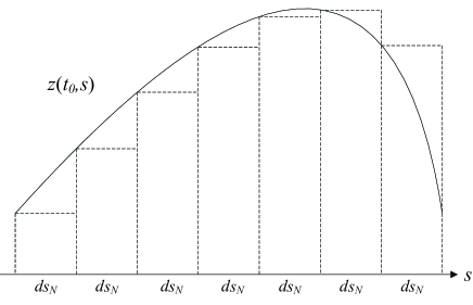
Figure 6: The PDE solution $z(t,s)$, at $t=t_{o}$ approximating the normalized queue lengths of a one-dimensional network.

IV-B2 Comparison between PDE approximation and Monte Carlo simulation: One dimension

We compare the PDE approximation obtained from our approach with the Monte Carlo simulations for a network over the domain $\mathcal{D}=[-1,1]$. We use the initial condition $z_{0}(s)=l_{1}e^{-s^{2}}$, where $l_{1}>0$ is a constant, so that initially the nodes in the middle have messages to transmit, while those near the boundaries have very few. We set the message generation rate $g_{p}(s)=l_{2}e^{-s^{2}}$, where $l_{2}>0$ is a parameter determining the total load of the system.

We use three sets of values of $N=20,50,80$ and $M=N^{3}$, and show the PDE solution and the Monte Carlo simulation results with different $N$ and $M$ at $t=1s$. The networks have diffusion coefficient $b=1/2$ and convection coefficient $c=0$ in Fig. 7 and $c=1$ in Fig. 8, respectively, where the x-axis denotes the node location and y-axis denotes the normalized queue length.

For the three sets of the values of $N=20,50,80$ and $M=N^{3}$ and with $c=0$, the maximum absolute errors of the PDE approximation are $5.6\times 10^{-3}$, $1.3\times 10^{-3}$, and $1.1\times 10^{-3}$, respectively; and with $c=1$, the errors are $4.4\times 10^{-3}$, $1.5\times 10^{-3}$, and $1.1\times 10^{-3}$, respectively. As we can see, as $N$ and $M$ increase, the resemblance between the Monte Carlo simulations and the PDE solution becomes stronger. In the case of very large $N$ and $M$, it is difficult to distinguish the results.

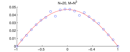
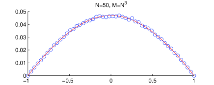
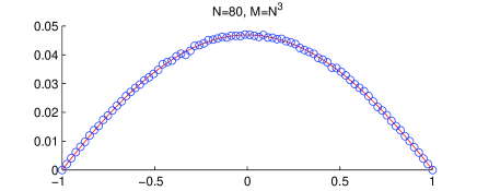
$\circ$ Monte Carlo simulation         —— PDE solution

Figure 7: The Monte Carlo simulations (with different $N$ and $M$) and the PDE solution of a one-dimensional network, with $b=1/2$ and $c=0$, at $t=1s$.

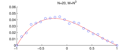
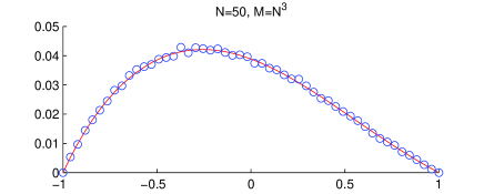
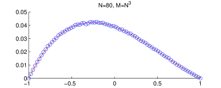
$\circ$ Monte Carlo simulation         —— PDE solution

Figure 8: The Monte Carlo simulations (with different $N$ and $M$) and the PDE solution of a one-dimensional network, with $b=1/2$ and $c=1$, at $t=1s$.

We stress that the PDEs only took fractions of a second to solve on a computer, while the Monte Carlo simulations took time on the order of tens of hours. We could not do Monte Carlo simulations of any larger networks because of prohibitively long computation time.

IV-C Continuum Model in Two Dimensions

Generalization of the continuum model to higher dimensions is straightforward, except for more arduous algebraic manipulation. Now we consider the two-dimensional network of $N_{1}\times N_{2}$ sensor nodes. The nodes are uniformly placed over the domain $\mathcal{D}\subset{\mathbb{R}}^{2}$ and labeled by $(n,m)$, where $n=1,\ldots,N_{1}$ and $m=1,\ldots,N_{2}$. Again let the distance between neighboring nodes be $ds_{N}$. Assume that the node at location $(n,m)$ randomly chooses to transmit to the north, east, south, or west immediate neighbor with probabilities $P_{e}(n,m)=b_{1}(s)+c_{e}(s)ds_{N}$, $P_{w}(n,m)=b_{1}(s)+c_{w}(s)ds_{N}$, $P_{n}(n,m)=b_{2}(s)+c_{n}(s)ds_{N}$, and $P_{s}(n,m)=b_{2}(s)+c_{s}(s)ds_{N}$, respectively. Define $c_{1}=c_{w}-c_{e}$ and $c_{2}=c_{s}-c_{n}$.

The derivation of the approximating PDE is similar to those of the one-dimensional cases, except that we now have to consider transmission to and interference from four directions instead of two. We present the approximating PDE here without the detailed derivation:

$$\dot{z} =\sum_{j=1}^{2}b_{j}\frac{\partial}{\partial s_{j}}\left((1+5z)(1-z)^{3}\frac{\partial z}{\partial s_{j}}\right)+2(1-z)^{3}\frac{\partial z}{\partial s_{j}}$$

$$\quad{}\times\frac{db_{j}}{ds_{j}}+z(1-z)^{4}\frac{d^{2}b_{j}}{ds_{j}^{2}}+\frac{\partial}{\partial s_{j}}\left(c_{j}z(1-z)^{4}\right),$$

with boundary condition $z(t,s)=0$ and initial condition $z(0,s)=z_{0}(s)$, where $t\in[0,T]$ and $s=(s_{1},s_{2})\in\mathcal{D}.$

IV-C1 Comparison between PDE approximation and Monte Carlo simulations: Two dimensions

We compare the PDE approximation and the Monte Carlo simulations of a network over the domain $D=[-1,1]\times[-1,1]$. We use the initial condition $z_{0}(s)=l_{1}e^{-(s_{1}^{2}+s_{2}^{2})}$, where $l_{1}>0$ is a constant, so that initially the nodes in the center have messages to transmit, while those near the boundary have very few. We set the message generation rate $g_{p}(s)=l_{2}e^{-(s_{1}^{2}+s_{2}^{2})}$, where $l_{2}>0$ is a parameter determining the total load of the system.

We use three different sets of the values of $N_{1}\times N_{2}$ and $M$, where $N_{1}=N_{2}=20,50,80$ and $M=N_{1}^{3}$. We show the contours of the normalized queue length from the PDE solution and the Monte Carlo simulation results with different sets of values of $N_{1}$, $N_{2}$, and $M$, at $t=0.1s$. The networks have diffusion coefficients $b_{1}=b_{2}=1/4$ and convection coefficients $c_{1}=c_{2}=0$ and $c_{1}=-2,c_{2}=-4$ in Fig. 9 and Fig. 10, respectively. It took 3 days to do the Monte Carlo simulation of the network at $t=0.1s$ with $80\times 80$ nodes and the maximum queue length $M=80^{3}$, while the PDE solved on the same machines took less than a second. We could not do Monte Carlo simulations of any larger networks or greater values of $t$.

For the three sets of values of $N_{1}=N_{2}=20,50,80$ and $M=N_{1}^{3}$ and with $c_{1}=c_{2}=0$, the maximum absolute errors are $3.2\times 10^{-3}$, $1.1\times 10^{-3}$, and $6.8\times 10^{-4}$, respectively; and with $c_{1}=-2,c_{2}=-4$, the errors are $4.1\times 10^{-3}$, $1.0\times 10^{-3}$, and $6.6\times 10^{-4}$, respectively. Again the accuracy of the continuum model increases with $N_{1}$, $N_{2}$, and $M$.

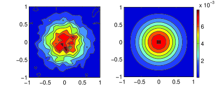
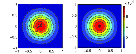
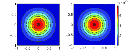
Monte Carlo simulations                      PDE solution

Figure 9: The Monte Carlo simulations (from top to bottom, with $N_{1}=N_{2}=20,50,80$, respectively, and $M=N_{1}^{3}$) and the PDE solution of a two-dimensional network, with $b_{1}=b_{2}=1/4$ and $c_{1}=c_{2}=0$, at $t=0.1s$.

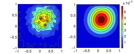
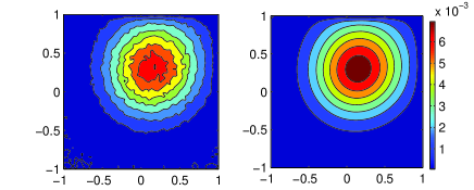
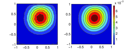
Monte Carlo simulations                      PDE solution

Figure 10: The Monte Carlo simulations (from top to bottom, with $N_{1}=N_{2}=20,50,80$, respectively, and $M=N_{1}^{3}$) and the PDE solution of a two-dimensional network, with $b_{1}=b_{2}=1/4$ and $c_{1}=-2,c_{2}=-4$, at $t=0.1s$.

V Conclusion and Future Work

In this paper we analyze the convergence of a sequence of Markov chains to its continuum limit, the solution of a PDE, in a two-step procedure. We provide precise sufficient conditions for the convergence and the explicit rate of the convergence. Based on such convergence we approximate the Markov chain modeling a large wireless sensor network by a nonlinear diffusion-convection PDE.

With the sophisticated mathematical tools available for PDEs, this approach provides a framework to model and simulate networks with a very large number of components, which is practically infeasible for Monte Carlo simulation. Such a tool enables us to tackle problems such as performance analysis and prototyping, resource provisioning, network design, network parametric optimization, network control, network tomography, and inverse problems, for very large networks. For example, we can now use the PDE model to optimize some performance metric of a large network by adjusting the placement of destination nodes or the routing parameters (coefficients in convection terms), with relatively negligible computational overhead compared with that of the same task done by Monte Carlo simulation.

The approximation approach can be extended in future work with more specific considerations regarding the network, which can significantly affect the derivation of the continuum model. For example, we can seek to establish continuum models for other domains such as the Internet, cellular networks, and traffic networks; we can consider more boundary conditions other than sinks, including walls, semi-permeating walls, and their composition; the nodes could be nonuniformly located, even mobile; transmission could happen between nodes that are not immediate neighbors; and the interference between nodes could behave differently in the presence of power control.

References

- [1] R. M. Fujimoto, K. S. Perumalla, and G. F. Riley, Network Simulation. Morgan & Claypool Publishers, 2007.
- [2] R. Bagrodia, R. Meyer, M. Takai, Y. A. Chen, X. Zeng, J. Martin, and H. Y. Song, “Parsec: a parallel simulation environment for complex systems,” Computer, vol. 31, no. 10, pp. 77 –85, Oct. 1998.
- [3] H. Plesser, J. Eppler, A. Morrison, M. Diesmann, and M. O. Gewaltig, “Efficient parallel simulation of large-scale neuronal networks on clusters of multiprocessor computers,” in Euro-Par 2007 Parallel Processing.
- [4] H. J. Kushner, Approximation and Weak Convergence Methods for Random Processes, with Applications to Stochastic Systems Theory. Cambridge, MA: MIT Press, 1984.
- [5] R. Norberg, “Anomalous PDEs in Markov chains: Domains of validity and numerical solutions,” Finance and Stochastics, vol. 9, no. 4, pp. 519–537, October 2005. [Online]. Available: http://ideas.repec.org/a/spr/finsto/v9y2005i4p519-537.html
- [6] R. W. R. Darling and J. R. Norris, “Differential equation approximations for Markov chains,” Probability Surveys, vol. 5, p. 37, 2008. [Online]. Available: doi:10.1214/07-PS121
- [7] E. K. P. Chong, D. Estep, and J. Hannig, “Continuum modeling of large networks,” Int. J. Numer. Model., vol. 21, no. 3, pp. 169–186, 2008.
- [8] S. L. Sobolev, Partial Differential Equations of Mathematical Physics. Courier Dover Publications, 1964.
- [9] R. G. Mortimer, Mathematics for Physical Chemistry. Academic Press, 2005.
- [10] M. Gillman, An Introduction to Mathematical Models in Ecology and Evolution: Time and Space. Wiley-Blackwell, 2009.
- [11] T. Hens and M. O. Rieger, Financial Economics. Springer, 2010.
- [12] G. R. Liu and S. S. Quek, The Finite Element Method: A Practical Course. Butterworth-Heinemann, 2003.
- [13] A. R. Mitchell and D. F. Griffiths, The Finite Difference Method in Partial Differential Equations. Wiley, 1980.
- [14] E. W. C. v. Groesen and J. Molenaar, Continuum Modeling in the Physical Sciences. Society for Industrial and Applied Mathematics, 2007.
- [15] H. B. Mühlhaus, Continuum Models for Materials with Microstructure. Wiley, 1995.
- [16] W. F. Phillips, A New Continuum Model for Traffic Flow. U.S. Dept. of Transportation, Research and Special Programs Administration National Technical Information Service [distributor], 1981.
- [17] D. Grünbaum, “Translating stochastic density-dependent individual behavior with sensory constraints to an Eulerian model of animal swarming,” J Math Biol, vol. 33, pp. 139–161, 1994.
- [18] J. M. Harrison, “Heavy traffic analysis of a system with parallel servers: Asymptotic optimality of discrete-review policies,” The Annals of Applied Probability, vol. 8, no. 3, pp. pp. 822–848, 1998. [Online]. Available: http://www.jstor.org/stable/2667208
- [19] J. G. Dai and J. M. Harrison, “Reflecting brownian motion in three dimensions: A new proof of sufficient conditions for positive recurrence,” Mathematical Methods of Operations Research, 2009.
- [20] M. Bramson, J. G. Dai, and J. M. Harrison, “Positive recurrence of reflecting Brownian motion in three dimensions,” ArXiv e-prints, Sep. 2010.
- [21] P. Gupta and P. R. Kumar, “The capacity of wireless networks,” Information Theory, IEEE Transactions on, vol. 46, no. 2, pp. 388–404, Mar 2000.
- [22] E. W. Grundke and A. N. Z. Heywood, “A uniform continuum model for scaling of ad hoc networks,” in ADHOC-NOW, 2003, pp. 96–103.
- [23] R. Bakhshi, L. Cloth, W. Fokkink, and B. R. Haverkort, “Meanfield analysis for the evaluation of gossip protocols,” SIGMETRICS Perform. Eval. Rev., vol. 36, pp. 31–39, November 2008. [Online]. Available: http://doi.acm.org/10.1145/1481506.1481513
- [24] M. E. J. Newman, C. Moore, and D. J. Watts, “Mean-field solution of the small-world network model,” Physical Review Letters, vol. 84, pp. 3201–3204, Apr. 2000.
- [25] R. B. Guenther and J. W. Lee, Partial Differential Equations of Mathematical Physics and Integral Equations. Mineola, NY: Courier Dover Publications, 1996.
- [26] T. C. Gard, Introduction to Stochastic Differential Equations (Pure and Applied Mathematics). Marcel Dekker Inc, 1987.
- [27] H. J. Kushner and G. G. Yin, Stochastic Approximation and Recursive Algorithms and Applications. Springer, 2003.
- [28] P. Billingsley, Probability and Measure. New York, NY: Wiley, 1995.