Extremal extensions of entanglement witnesses : Unearthing new bound entangled states

Abstract

In this paper, we discuss extremal extensions of entanglement witnesses based on Choi’s map. The constructions are based on a generalization of the Choi map due to Osaka, from which we construct entanglement witnesses. These extremal extensions are powerful in terms of their capacity to detect entanglement of positive under partial transpose (PPT) entangled states and lead to unearthing of entanglement of new PPT states. We also use the Cholesky-like decomposition to construct entangled states which are revealed by these extremal entanglement witnesses.

I Introduction

Quantum entanglement plays a central role in quantum theory from a conceptual as well as a practical point of view. On the conceptual front, entanglement is intimately connected with the notions of non-locality and violation of Bell’s inequalities, which lie at the heart of the way the quantum mechanical description of the world differs from the classical one. On the practical front, quantum entanglement is essential in providing a computational advantage to quantum computers over their classical counterparts Nielsen and Chuang (2000).

The quantum state of a physical system with a finite-dimensional complex Hilbert space $H$ (which is either pure or mixed), is represented by $\rho\in\mathcal{B}(H)$ which is a positive semi-definite hermitian operator with unit trace. The set of states forms a convex set and the extremal points of this set are pure states which are operators of rank 1.

For composite quantum systems, the Hilbert space is the tensor product of Hilbert spaces of the individual systems. Consider a bipartite quantum system with its state space given by $H_{A}\otimes H_{B}$ where $H_{A}$ and $H_{B}$ are the Hilbert spaces of individual quantum system. A bipartite state $\rho_{AB}\in\mathcal{B}(H_{A}\otimes H_{B})$ is said to be separable if it is possible to decompose it as follows:

$$\rho_{AB}=\sum_{j=1}^{m}p_{j}\rho_{A_{j}}\otimes\rho_{B_{j}};\quad\forall j~{}~{}p_{j}>0,\quad\sum_{j=1}^{m}p_{j}=1;$$ (1)

where $\rho_{A_{j}}$ and $\rho_{B_{j}}$ are states in systems $A$ and $B$ respectively. A bipartite state $\rho\in\mathcal{B}(H_{A}\otimes H_{B})$ is said to be entangled if it is not separable i.e. it cannot be expanded in the form given in Equation (1).

For pure quantum states, the characterization of states as separable or entangled, is easily achieved by computing the entropy of the reduced density operator of the subsystems. However, such a characterization for mixed states is a non-trivial problem. While a large volume of work has appeared on this issue in the past two decades, the problem still remains open. In the absence of a “final solution”, explorations into finding new classes of mixed entangled states and new ways of constructing them, is useful and provides insights into the classification problem.

An important method to detect the entanglement of quantum states is to construct entanglement witnesses, which are positive maps that are not completely positive Horodecki et al. (1996). Consider a positive map $h_{A}$ defined on the Hilbert space $H_{A}$ of system $A$. If this map is not completely positive, then for some $H_{B}$ the map $h_{A}\otimes I$ acting on $H_{A}\otimes H_{B}$ will not be positive. Therefore, there will be a state $\rho_{AB}$ for which $(h_{A}\otimes I)\rho_{AB}$ will be negative. However, this cannot happen for a separable state defined in (1). Therefore, such a $\rho_{AB}$ has to be entangled.

Partial transposition was the first such entanglement witness which was used to unearth the entanglement of pure as well as mixed states Peres (1996); Horodecki et al. (1996). While negativity under partial transpose (NPT) indicates entanglement, positivity under partial transpose is both necessary and sufficient only for $2\otimes 2$ and $2\otimes 3$ systems. The proof relied on the earlier works of Woronowicz Woronowicz (1976a), Arvison Arveson (1969, 1974) and Størmer Størmer (1963, 1982) where they show that in dimension 2, all positive but not completely positive maps are decomposable (can be written as a combination of a completely positive map and a transposed completely positive map). A corollary of their result shows that, for dimensions $2\otimes 2$ and $2\otimes 3$, a state is separable if and only if it remains positive under partial transpose. However in higher dimensions there could be maps which are positive but not completely positive and which may not have a connection with partial transpose. This means that there could be states which are positive under partial transpose (PPT) and are still entangled. Such states are called PPT entangled states. Obviously for such states, there exists a positive but not completely positive map revealing their entanglement Jamiołkowski (1972); Woronowicz (1976a, b); Horodecki et al. (2009); Gühne and Tóth (2009).

Choi provided the first example of an indecomposable map which later led to the detection of entangled states beyond partial transpose Choi (1975a). A number of other discrete examples are also available Cho et al. (1992); Ha (1998); Osaka (1992); Ha (2002, 1998); Terhal (2001); Robertson (1983a, b, c, 1985). However there is no systematic way of characterizing such maps beyond two dimensions. A few methods have been recently suggested for generating examples of positive maps which are not completely positive Kossakowski (2003); Kimura and Kossakowski (2004). However, there is no straight forward procedure to verify if they are indecomposable or not. Generalizations of Choi’s method have also been adopted to produce indecomposable maps which in principle have the potential to reveal entanglement of new quantum states Chruściński and Kossakowski (2007).

The present paper is an attempt in this direction, where we have constructed extremal extensions of known entanglement witnesses in order to unearth new classes of bound entangled states. We have constructed examples of PPT entangled states which are revealed by extremal Choi type maps considered by Choi and Lam Choi and Lam (7778), and later by OsakaOsaka (1992), and have exploited the Cholesky decomposition in a nontrivial way. The Cholesky decomposition has been used by Chruściński et al. Chruściński et al. (2008) in the context of PPT states; however our analysis goes much beyond that. Moreover, given any extremal positive but not completely positive map, we can use our method to generate new classes of extremal maps. In particular, for the $3\otimes 3$ bipartite system, we have constructed PPT states whose entanglement is revealed by our map but is not revealed by Choi’s map. For the positive maps which are not completely positive, the question of extremality has been settled only for a few maps and the problem of determining the structure of such maps and their extremal or non-extremal nature is in general difficult. In this regard, we believe that our generalization adds new insights into the class of extremal entangled witnesses. Further, for a given map which is positive but not completely positive, it is not always trivial to find the PPT entangled states revealed by the map. In our case we were able to find a family of such states.

The material in this paper is arranged as follows: In section II we discuss the bi-quadratic forms and their connection with positive maps, where the notions of extremality and decomposability are discussed as important ingredients for the purpose of classification of entangled states. In section III we explore the possibility of extremal extensions of Choi’s map. We present Osaka’s map as an extremal extension of Choi’s map and go on to construct other extremal extensions. We then turn to constructing examples of bound entangled states whose entanglement is revealed by Osaka’s map and by our new extremal extension of Choi’s map. At the end of this section we show that the bound entangled states that we have constructed are robust and can take a certain amount of noise before they lose their entanglement. Section IV offers some concluding remarks.

II Bi-quadratic forms and extremal Maps

Given a non-negative polynomial $P(x_{1},\cdots,x_{n})\geq 0,~{}\forall(x_{1},\cdots,x_{n})\in\mathbb{R}^{n}$ of degree $d$, the question whether $P$ can always be written as a sum of squares of polynomials has been around for a long time. Minkowski conjectured that in general the answer should be ‘no’. It was proved by Hilbert that, except for three exceptional cases ($n=1$, $d$ arbitrary; $n$ arbitrary, $d=2$; and one non-trivial case $n=2$, $d=4$), there always exist positive semi-definite polynomials which cannot be written as a sum of squares of polynomials. However, his proof was by an indirect method and did not provide actual examples of such polynomials. For a survey and development of the problem, see Rudin Rudin (2000). The generalized version of this problem on rational polynomials, is known as Hilbert’s 17th problem, and for which the answer is ‘yes’.

The first counterexample was constructed by Choi Choi (1975a) where he considered a positive semi-definite bi-quadratic form $F_{\mu}(X:Y)$ (each term having degree four), with six variables, divided into two sets denoted by $X=\{x_{1},x_{2},x_{3}\}$, and $Y=\{y_{1},y_{2},y_{3}\}$ given by:

$$F_{\mu}(X:Y) = (x_{1}^{2}y_{1}^{2}+x_{2}^{2}y_{2}^{2}+x_{3}^{2}y_{3}^{2})$$ (2)

$$-2(x_{1}x_{2}y_{1}y_{2}+x_{2}x_{3}y_{2}y_{3}+x_{3}x_{1}y_{3}y_{1})$$

$$+\mu(x_{1}^{2}y_{2}^{2}+x_{2}^{2}y_{3}^{2}+x_{3}^{2}y_{1}^{2})$$

where $\mu\geq 1$.

Choi proved that for $\mu>1$, this bi-quadratic form is non-negative definite but cannot be written as a sum of squares of quadratic forms Choi (1975a). Later it was shown by Choi and Lam Choi and Lam (7778) that it is also true for $\mu=1$. Choi’s method has been modified and extended, and different examples of such positive semi-definite bi-quadratic forms were found. Among these, the results by Osaka Osaka (1992), Cho et. al. Cho et al. (1992), and Ha Ha (2003, 1998, 2002) are important. Later generalizations of these methods for generating such forms in arbitrary dimensions were developed by Chruściński and Kossakowski Chruściński and Kossakowski (2007).

II.1 Connection with positive maps

The intimate connection between a positive map and positive semi-definite bi-quadratic forms was also discovered by Choi Choi (1975a). Before describing the connection we provide a few definitions.

Definition :  A hermiticity preserving map $h:M_{n}(\mathbb{C})\longrightarrow M_{n}(\mathbb{C})$, is said to be a positive map, if it maps positive semi- definite operators to positive semi-definite operators. Here $M_{n}(\mathbb{C})$ denotes the set of all $n\times n$ complex matrices.

Definition :  A positive map $h$ is said to be $k$-positive if the extended map

$$h\otimes\mathbf{1}_{k}:M_{k}(\mathbb{C})\otimes M_{n}(\mathbb{C})\longrightarrow M_{k}(\mathbb{C})\otimes M_{n}(\mathbb{C}),$$

is positive, we here $\mathbf{1}_{k}$ denotes the identity mapping on the auxiliary space $M_{k}(\mathbb{C})$. The map $h$ is said to be completely positive if the above extensions are positive for all $k\geq 1$.

The connection between the maps and bi-quadratic forms can be established as follows. Consider a hermiticity preserving linear map

$$S:\mathbb{C}_{m}\rightarrow\mathbb{C}_{n},$$ (3)

We can construct the corresponding bi-quadratic form $F(X:Y)$ as

$$F(X:Y)=\langle Y|S(X\cdot X^{T})|Y\rangle$$ (4)

where $X=\begin{pmatrix}x_{1}\cdots x_{m}\end{pmatrix}^{T}$ and $Y=\begin{pmatrix}y_{1}\cdots y_{n}\end{pmatrix}^{T}$.

On the other hand, let $F(X:Y)$ be a bi-quadratic form. Notice that, it is a quadratic form with respect to $Y$ (as well as $X$). So we can write it in the form $\langle Y|A_{X}|Y\rangle$. Thus we get a map which takes any one-dimensional projection $X.X^{T}$ to $A_{X}$. Using linearity and hermiticity, we can extend it to a map which preserves hermiticity. It was shown by Choi that, given any positive semi-definite form, the corresponding map is a positive map and vice-versa Choi (1980, 1975a).

There is thus a bijective relation between the set of positive semi-definite forms and positive maps between matrix algebras. The property of complete positivity can also be translated easily. If a map is completely positive, the corresponding bi-quadratic form can be written as a sum of squares of quadratic forms and vice versa. Put differently, if a map is positive but not completely positive, the corresponding bi-quadratic form will be positive semi-definite but can not be written as a sum of squares of quadratic forms. Thus each such form gives rise to a unique map between the space of real symmetric operators, which can be trivially extended to the set of all hermitian operators, and then to all operators. This also connects with the work of Arvison Arveson (1969, 1974) and Størmer Størmer (1963, 1982) who were exploring the set of positive maps between $C^{*}$-algebras. Since then, other examples and classes of such maps have been discovered.

By the above correspondence, the Choi quadratic form given in Equation  (2) leads to the following map for $3\times 3$ matrices.

$$\Phi_{C}^{I}(\mu): \begin{pmatrix}a_{11}&a_{12}&a_{13}\\ a_{21}&a_{22}&a_{23}\\ a_{31}&a_{32}&a_{33}\end{pmatrix}\mapsto$$ (5)

$$\begin{pmatrix}a_{11}+\mu a_{33}&-a_{12}&-a_{13}\\ -a_{21}&a_{22}+\mu a_{11}&-a_{23}\\ -a_{31}&-a_{32}&a_{33}+\mu a_{22}\end{pmatrix},$$

with $\mu\geq 1$. From the quadratic form (2), exchanging the $X$ and $Y$ variables, we can get another map, which is given by

$$\Phi_{C}^{II}(\mu): \begin{pmatrix}a_{11}&a_{12}&a_{13}\\ a_{21}&a_{22}&a_{23}\\ a_{31}&a_{32}&a_{33}\end{pmatrix}\mapsto$$ (6)

$$\begin{pmatrix}a_{11}+\mu a_{22}&-a_{12}&-a_{13}\\ -a_{21}&a_{22}+\mu a_{33}&-a_{23}\\ -a_{31}&-a_{32}&a_{33}+\mu a_{11}\end{pmatrix}.$$

Our interest in these positive but not completely positive maps is because of their ability to detect entanglement of quantum states. For the maps that are to be used as entanglement witnesses, two notions, namely decomposability and extremality are very important. We define these notions below.

Definition :  A positive but not completely positive map is called decomposable, if it can be written as a sum of a completely positive and a completely co-positive map.

This property was first discussed by Woronowicz Woronowicz (1976a). Since decomposable maps are obtained by combining a completely positive map with a transposed completely positive map, it is clear that they are weaker than partial transpose in terms of their ability to detect entanglement and therefore are not of interest. The interesting point however is that, given a map which is positive but not completely positive, there is no standard way to check if it is decomposable or not!

Since the set of positive maps is a convex set it can be described by its extremal elements. Therefore, it is most natural to study extremal positive maps. From the point of view of detecting entanglement, any extremal map is more powerful than the maps which are internal points of the set of positive maps Choi and Lam (7778); Osaka (1992). Choi and Lam define an extremal map using the corresponding bi-quadratic form Choi and Lam (7778) as follows.

Definition :  A positive semi-definite bi-quadratic form $F$ is said to be extremal if, for any decomposition of $F=F_{1}+F_{2}$ where $F_{i}$’s are positive semi-definite bi-quadratic forms, $F_{i}=\lambda_{i}F$, where $\lambda_{1},~{}\lambda_{2}$ are non-negative real numbers with $\lambda_{1}+\lambda_{2}=1$.

It was shown by Choi and Lam that in the case $\mu=1$, the form $F_{1}$ defined in Equation (2) is extremal.

Since the set of positive semi-definite forms is a convex set, it is enough to identify the set of such extremal forms. At this stage it is useful to change the notation to the original Choi-Lam notation for the bi-quadratic forms and we therefore denote $F(X:Y)$ as $F\begin{pmatrix}x_{1}&x_{2}&x_{3}\\ y_{1}&y_{2}&y_{3}\end{pmatrix}$.

III Extremal maps and bound entangled states

Osaka extended the result of Choi and Lam, and generated a class of extremal maps Osaka (1992). Osaka’s map $\Phi_{O}(x,y,z)$ is defined as

$$\Phi_{O}(x,y,z): \begin{pmatrix}a_{11}&a_{12}&a_{13}\\ a_{21}&a_{22}&a_{23}\\ a_{31}&a_{32}&a_{33}\end{pmatrix}\mapsto$$ (7)

$$\begin{pmatrix}a_{11}+xa_{33}&-a_{12}&-a_{13}\\ -a_{21}&a_{22}+ya_{11}&-a_{23}\\ -a_{31}&-a_{32}&a_{33}+za_{22}\end{pmatrix},$$

where $x,y,z>0$ and $xyz=1$. Osaka showed that this class of maps is extremal Osaka (1992).

Generalizing beyond Osaka construction, we define a class of extremal bi-quadratic forms as follows:

Let $F=F\begin{pmatrix}x_{1}&x_{2}&x_{3}\\ y_{1}&y_{2}&y_{3}\end{pmatrix}$ be an extremal positive semi-definite bi-quadratic form.

For a set of non-zero positive real numbers $a,b,c$ we define

$$G\begin{pmatrix}x_{1}&x_{2}&x_{3}\\ y_{1}&y_{2}&y_{3}\end{pmatrix}=F\begin{pmatrix}ax_{1}&bx_{2}&cx_{3}\\ y_{1}&y_{2}&y_{3}\end{pmatrix}$$ (8)

It turns out that the form $G\begin{pmatrix}x_{1}&x_{2}&x_{3}\\ y_{1}&y_{2}&y_{3}\end{pmatrix}$ is positive semi-definite and extremal.

Proof :  We first prove the positivity. Let us assume that the proposition is not true and there exists real numbers $p_{1},p_{2},p_{3},q_{1},q_{2},q_{3}$ such that $G\begin{pmatrix}p_{1}&p_{2}&p_{3}\\ q_{1}&q_{2}&q_{3}\end{pmatrix}<0$. But then by definition $F\begin{pmatrix}p_{1}^{\prime}&p_{2}^{\prime}&p_{3}^{\prime}\\ q_{1}&q_{2}&q_{3}\end{pmatrix}<0$; for a set of real numbers $p_{1}^{\prime},p_{2}^{\prime},p_{3}^{\prime},q_{1},q_{2},q_{3}$ where $p_{1}^{\prime}=ap_{1},~{}p_{2}^{\prime}=bp_{2}$ and $p_{3}^{\prime}=cp_{3}$. This contradicts the assumption that $F$ is a positive semi-definite form for all real values of $x_{i}$’s and $y_{j}$’s.

For extremality, let us assume $G=G_{1}+G_{2}$, where $G_{1}$ and $G_{2}$ are positive semi-definite bi-quadratic forms.

Notice that

$$F\begin{pmatrix}x_{1}&x_{2}&x_{3}\\ y_{1}&y_{2}&y_{3}\end{pmatrix} = G\begin{pmatrix}\frac{x_{1}}{a}&\frac{x_{2}}{b}&\frac{x_{3}}{c}\\ y_{1}&y_{2}&y_{3}\end{pmatrix}$$

$$= G_{1}\begin{pmatrix}\frac{x_{1}}{a}&\frac{x_{2}}{b}&\frac{x_{3}}{c}\\ y_{1}&y_{2}&y_{3}\end{pmatrix}+G_{2}\begin{pmatrix}\frac{x_{1}}{a}&\frac{x_{2}}{b}&\frac{x_{3}}{c}\\ y_{1}&y_{2}&y_{3}\end{pmatrix},$$

as we have assumed. Define two positive semi-definite forms

$$F_{i}\begin{pmatrix}x_{1}&x_{2}&x_{3}\\ y_{1}&y_{2}&y_{3}\end{pmatrix}=G_{i}\begin{pmatrix}\frac{x_{1}}{a}&\frac{x_{2}}{b}&\frac{x_{3}}{c}\\ y_{1}&y_{2}&y_{3}\end{pmatrix},$$

for $i=1,2$. We can now write,

$$F=F_{1}+F_{2}.$$

However, $F$ is extremal. Therefore, $F_{i}=\lambda_{i}F,~{}i=1,~{}2$, and $\lambda_{1}$ and $\lambda_{2}$ are positive real numbers with $\lambda_{1}+\lambda_{2}=1$. Thus $G_{i}\begin{pmatrix}\frac{x_{1}}{a}&\frac{x_{2}}{b}&\frac{x_{3}}{c}\\ y_{1}&y_{2}&y_{3}\end{pmatrix}=\lambda_{i}F\begin{pmatrix}x_{1}&x_{2}&x_{3}\\ y_{1}&y_{2}&y_{3}\end{pmatrix}$. Hence

$$G_{i}\begin{pmatrix}x_{1}&x_{2}&x_{3}\\ y_{1}&y_{2}&y_{3}\end{pmatrix} = G_{i}\begin{pmatrix}a\frac{x_{1}}{a}&b\frac{x_{2}}{b}&c\frac{x_{3}}{c}\\ y_{1}&y_{2}&y_{3}\end{pmatrix}$$

$$= \lambda_{i}F\begin{pmatrix}ax_{1}&bx_{2}&cx_{3}\\ y_{1}&y_{2}&y_{3}\end{pmatrix}$$

$$= \lambda_{i}G.$$

Since $\lambda_{1},~{}\lambda_{2}\geq 0$ and $\lambda_{1}+\lambda_{2}=1$; the form $G$ is an extremal form.

The maps corresponding to the bi-quadratic form $G$ defined above are positive maps which are extremal. This construction is extendable to higher dimensions without any further work. This means that given any extremal positive semi-definite bi-quadratic form, $F=F\begin{pmatrix}x_{1}&x_{2}&\cdots&x_{n}\\ y_{1}&y_{2}&\cdots&y_{n}\end{pmatrix}$, for any non zero positive real $a_{1},a_{2},\cdots,a_{n}$; $G=F\begin{pmatrix}a_{1}x_{1}&a_{2}x_{2}&\cdots&a_{n}x_{n}\\ y_{1}&y_{2}&\cdots&y_{n}\end{pmatrix}$ is positive semi-definite and extremal.

We now turn to the map corresponding to the extremal bi-quadratic form $G$ from Equation (2). After working out the details, the map turns out to be

$$\Phi(a,b,c): \begin{pmatrix}x_{11}&x_{12}&x_{13}\\ x_{21}&x_{22}&x_{23}\\ x_{31}&x_{32}&x_{33}\end{pmatrix}\mapsto$$ (9)

$$\!\!\!\!\!\!\!\!\!\!\!\!\!\!\!\begin{pmatrix}a^{2}x_{11}+c^{2}x_{33}&-abx_{12}&-acx_{13}\\ -abx_{21}&b^{2}x_{22}+a^{2}x_{11}&-bcx_{23}\\ -acx_{31}&-bcx_{32}&c^{2}x_{33}+b^{2}x_{22}\end{pmatrix}$$

where $a,b,c\neq 0$. The map $\Phi(a,b,c)$ is an extremal positive map which may not be completely positive. For the values of $a,b$ and $c$ for which it is not completely positive, it can act as an entanglement witness.

We now construct a set of PPT entangled states for which the above map acts as an entanglement witness. Consider a density operator for a $3\otimes 3$ system defined by two parameters $t$ and $x$.

$$\rho(x,t)=\frac{1}{4+\frac{3}{t}+4t}\left(\begin{array}[]{ccc|ccc|ccc}1+t&0&0&0&x&0&0&0&x\\ 0&t&0&x&0&0&0&0&0\\ 0&0&\frac{1}{t}&0&0&0&x&0&0\\ \hline\cr 0&x&0&\frac{1}{t}&0&0&0&0&0\\ x&0&0&0&1+t&0&0&0&x\\ 0&0&0&0&0&t&0&x&0\\ \hline\cr 0&0&x&0&0&0&1&0&0\\ 0&0&0&0&0&x&0&\frac{1}{t}&0\\ x&0&0&0&x&0&0&0&1\end{array}\right).$$ (10)

This $\rho$ is a unit trace density operator for $t>0$ and $0\leq x\leq 1$.

The action of the map $\Phi(a,b,c)$ on the density operator $\rho(x,t)$ leads to the transformed density operator $\rho^{x,}$.

$$\rho^{\prime}(x,t)=(\Phi(a,b,c)\otimes\mathbf{1}_{3})\rho(x,t).$$ (11)

We compute eigenvalues of $\rho(x,t)^{\prime}$ and use the negativity of the least eigenvalue as an indicator of entanglement of $\rho(x,t)$. It is useful to note that the map $\Phi(a,b,c)$ with, $a=b=c=1$ reduces to Choi’s map $\Phi_{C}^{I}(1)$ while for other values of $a,b$ and $c$ it is still an extremal map with a potential to reveal entanglement of quantum states.

A computation of eigenvalues of $\rho^{\prime}(x,t)$ reveals that for this example, the maps $\Phi(a,b,c)$ have more potential than Choi’s map in unearthing the entanglement of PPT quantum states. The results are displayed graphically in Figures 1 and 2. We take the parameter values to be $a=1+\frac{3}{5}$, $b=c=1$ and calculate the minimum eigenvalues of $\rho(x,t)$ for the range $x\in[0,1]$ and $t\in(0,1]$. The results are displayed in Figure 1. The curved surface denotes the minimum eigenvalue of $\rho(x,t)$ after the action $\Phi(1+\frac{3}{5},1,1)$. To show the power of this map clearly, we display a section of the above graph where we fix the parameter $x=\frac{1}{20}$ and plot the minimum eigenvalue as a function of $t$. We compare our result with Choi’s maps. The result is shown in Figure 2. The continuous line here denotes the minimum eigenvalue corresponding to the action $\Phi(1+\frac{3}{5},1,1)$ while the other two dashed lines are the minimum eigenvalues corresponding to $\Phi_{C}^{I}$ and $\Phi_{C}^{II}$. It turns out that approximately after $x=0.604428$, the minimum eigenvalue becomes negative under $\Phi(1+\frac{3}{5},1,1)$ while the minimum eigenvalues under $\Phi_{C}^{I}(1)$ and $\Phi_{C}^{II}(1)$ still remain positive. It is only after $x$ crosses the value $0.66$ that Choi’s maps begin to detect entanglement for this class of states. Therefore, for $\rho(x,\frac{1}{20})$, there is a clear window of $x$ values where the entanglement is revealed by $\Phi(1+\frac{3}{5},1,1)$ and is not revealed by any of the Choi’s maps.

The map $\Phi(1+\frac{3}{5},1,1)$ was chosen as a representative example. In fact the class of maps $\Phi(a,b,c)$ can reveal the entanglement of a large class of PPT entangled states and therefore provide a genuine extremal extension of Choi’s maps.

\psfrag{t}{\large$t$}\psfrag{x}{\large$x$}\includegraphics[width=213.39566pt]{sengupta_fig1.eps}

Figure 1: The plot of least eigenvalues of $\rho^{\prime}(x,t)$ as a function of $x$ and $t$. The curved surface corresponds to the case where $\rho^{\prime}(x,t)$ was generated by the action of $\Phi(1+\frac{3}{5},1,1)$ upon $\rho(x,t)$. The middle plane is the plane $xy=0$, given a referral plane for highlighting the negativity of the eigenvalues represented by the curved surface.

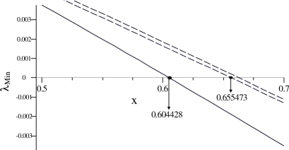
Figure 2: The section corresponding to $t=\frac{1}{20}$ of Figure 1 is displayed here. The blue line corresponds to the map $\Phi(1+\frac{3}{5},1,1)$ while the other two curves correspond to the two Choi’s maps. The window of values of $x$ (approximately $x\geq 0.6025$ and $x<0.66$) where the map $\Phi(1+\frac{3}{5},1,1)$ is able to reveal the entanglement of $\rho(x,t)$ and where Choi’s maps do not reveal the entanglement is clearly visible.

III.1 PPT entangled states detected by Osaka’s map

We now address the question of constructing PPT entangled states for which Osaka’s map acts as an entanglement witness. Although the three-parameter family of maps due to Osaka as described in Equation 7 has been defined, and is known to be positive but not completely positive, there has not been an explicit construction of PPT entangled states whose entanglement is revealed by this class of maps.

We set up a computer search over the PPT entangled states and employ the Cholesky decomposition Bhatia (2007) to selectively scan the states in the Hilbert space. We also make an intelligent use of Choi-Jamiołkowski isomorphism developed in Choi (1975b, a); Jamiołkowski (1972); Chruściński and Kossakowski (2008) to check at each stage of our search that the state remains entangled. This method of searching for entangled states for a given positive but not completely positive map is in fact more general and can be tried for other maps too.

According to the Cholesky decomposition, every density matrix $\rho$ of a quantum system can be decomposed as $\rho=T^{\dagger}T$, where $T$ is an upper triangular matrix Bhatia (2007). If $\rho$ is strictly positive (i.e. all eigenvalues are greater than zero), then the corresponding Cholesky Decomposition is unique. For simplicity, we restrict ourselves to the case of real states where elements of the density matrix are real and in this case the Cholesky decomposition reduces to $\rho=T^{t}T$, where $t$ denotes the transpose operation.

The Choi Jamiołkowski isomorphism developed in Choi (1975b, a); Jamiołkowski (1972); Chruściński and Kossakowski (2008) provides a simple one-way test of entanglement for a given positive map which is not completely positive. Consider a composite system $H_{1}\otimes H_{2}$ where both the subsystems are of dimension $d$. Using the standard basis $|i\rangle$ in both the $H_{1}$ and $H_{2}$ we define a maximally entangled state

$$|\psi\rangle=\frac{1}{\sqrt{d}}\sum_{i=0}^{d-1}|i\rangle\otimes|i\rangle;$$ (12)

Given a positive map $\Phi$ that is not completely positive we define an operator

$$W_{\Phi}=\frac{1}{\sqrt{d}}\sum_{i=0}^{d-1}|i\rangle\langle i|\otimes\varphi(|i\rangle\langle i|).$$ (13)

Given a density matrix $\rho$ defined on $H_{1}\otimes H_{2}$ the operator $W$ provides a sufficient condition for entanglement

$${\rm Tr}(W\rho)<0\Longrightarrow\quad\rho\quad{\rm Entangled}$$ (14)

This is a one-way condition and ${\rm Tr}(W\rho)\geq 0$ does not imply that the state $\rho$ is separable. The condition for entanglement given in (14) helps us in quickly identifying states whose entanglement is revealed by the map $\Phi$ and we employ this condition in our search for PPT entangled states revealed by Osaka family of maps.

We first construct a upper triangular matrix $T$. We further restrict to those states which are invariant under partial transpose by imposing the condition $(T^{t}T)^{PT}=T^{t}T$ (where $PT$ denotes the transpose with respect to the second system). This amounts to generating a non-trivial solution of the equation

$$(T^{t}T)^{PT}-T^{t}T=0.$$ (15)

It is not always possible to find a non-trivial solution to the above equation. However, if we begin with a sparse matrix $T$ we can hope to find a solution to the above equation. In our search we also at every stage impose the following condition

$$\left\{\begin{array}[]{l}\mathrm{Tr}\left(W\Phi_{O}\rho\right)<0\\ \mathrm{Tr}\left(W\Phi_{C^{I}}\rho\right)\geq 0\end{array}\right.$$ (16)

This means that we restrict ourselves to those PPT states whose entanglement is revealed by Osaka’s map but is not revealed by Choi’s map. The above methodology guides us in our computer search process to look for classes of states whose entanglement is revealed by the Osaka family of maps.

Using this method and employing a computer search protocol, we construct an example of a PPT entangled state for a $3\otimes 3$ system. The upper triangular matrix $T$ given by

$$\left(\begin{array}[]{ccccccccc}\sqrt{10}y&0&0&0&\frac{2+5y}{\sqrt{10}}&0&0&0&\frac{3(1+y)}{\sqrt{10}}\\ 0&y&0&2+5y&0&0&0&0&0\\ 0&0&3y&0&0&0&1+y&0&0\\ 0&0&0&0&0&0&0&0&0\\ 0&0&0&0&\frac{4+5y}{\sqrt{10}}&0&0&0&\frac{1+y}{\sqrt{10}}\\ 0&0&0&0&0&1+2y&0&1+y&0\\ 0&0&0&0&0&0&0&0&0\\ 0&0&0&0&0&0&0&0&0\\ 0&0&0&0&0&0&0&0&0\end{array}\right).$$ (17)

leads to a one parameter family of density operators, parameterized by a positive parameter $y$.

$$\rho(y)=\frac{1}{N}\times$$

$$\left[\!\!\begin{array}[]{ccccccccc}10y^{2}&0&0&0&y(2+5y)&0&0&0&3y(1+y)\\ 0&y^{2}&0&y(2+5y)&0&0&0&0&0\\ 0&0&9y^{2}&0&0&0&3y(1+y)&0&0\\ 0&y(2+5y)&0&(2+5y)^{2}&0&0&0&0&0\\ y(2+5y)&0&0&0&2+6y+5y^{2}&0&0&0&(1+y)(1+2y)\\ 0&0&0&0&0&(1+2y)^{2}&0&(1+y)(1+2y)&0\\ 0&0&3y(1+y)&0&0&0&(1+y)^{2}&0&0\\ 0&0&0&0&0&(1+y)(1+2y)&0&(1+y)^{2}&0\\ 3y(1+y)&0&0&0&(1+y)(1+2y)&0&0&0&(1+y)^{2}\end{array}\!\!\right]$$ (27)

(28)

where $N=10+36y+57y^{2}$ is the normalization factor such that $\mathrm{Tr}(\rho(y))=1$. We apply a one parameter subfamily of Osaka’s map defined in (7) $\Phi_{O}\left(1,x,\frac{1}{x}\right)$ to the family of states $\rho(y)$ and compute the eigenvalues of the resultant operator. We do a similar computation of the eigenvalues of the operator which is obtained by the action of Choi’s maps $\Phi_{C}^{I}$ and $\Phi_{C}^{I}I$ for comparison.

\psfrag{y}{\large$y$}\psfrag{x}{\large$x$}\includegraphics[width=213.39566pt]{sengupta_fig3.eps}

Figure 3: Application of Osaka’s map $\Phi_{O}\left(1,x,\frac{1}{x}\right)$ to the density operator $\rho(y)$. The two independent variables are $x$ and $y$, and the vertical axis denotes the eigenvalues of $\rho(y)$ under the map. The curved surface represents the variation of the minimum eigenvalue. The plane in the center is the plane $xy=0$, which highlights the portion of the surface with negative eigenvalue.

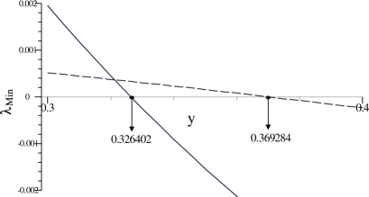
Figure 4: Application of Osaka’s map with $x=6$. The horizontal axis is $y$ and eigenvalues are along the vertical axis. The continuous line denotes the variation of eigenvalues under $\Phi_{O}\left(1,6,\frac{1}{6}\right)$. The dashed line corresponds to Choi’s map. It clearly shows that approximately after $y=0.326402$ onward, PPT entanglement is revealed by $\Phi_{O}(\left(1,6,\frac{1}{6}\right)$. However Choi’s map can reveal entanglement approximately from $y=0.369284$. This shows the superiority of Osaka’s map over Choi’s map for this instance of $\rho(y)$.

In Figure 3 the least eigenvalue is plotted as a function $x$ and $y$. Here the curved surface denotes the minimum eigenvalue corresponding to the $\Phi_{O}\left(1,x,\frac{1}{x}\right)$. The middle plane denotes the $xy$ plane which is placed to indicate the place when the surface becomes negative. In Figure 4 we have taken a fixed value of $x$. The eigenvalues are plotted along the vertical axis and $y$ varies along the horizontal axis. We apply the map $\Phi_{O}\left(1,6,\frac{1}{6}\right)$ to this state $\rho(y)$ and plot the minimum eigenvalue which is denoted by the continuous curve in Figure 4. The dashed curve denotes the minimum eigenvalue achieved by the Choi’s map. The plot highlights that approximately after point $y=0.326402$ the minimum eigenvalue under $\Phi_{O}\left(1,6,\frac{1}{6}\right)$ becomes negative. Thus there is a range of values, where Osaka’s map can identify more PPT entangled states while the Choi’s map fails to do so.

III.2 Robustness analysis

We now consider the robustness of the states given in Equations (28) and (10). Let $\rho$ be an arbitrary entangled state. We consider the convex combination of $\rho$ with a maximally mixed state. For this case we consider the following convex combination;

$$\rho^{\prime}(\varepsilon)=\frac{\varepsilon}{9}\mathbb{I}_{9}+(1-\varepsilon)\rho;$$

and try to detect the range of $\varepsilon$ for which $\rho^{\prime}$ is entangled. $\mathbb{I}_{9}$ denotes the identity matrix of dimension 9. Typically, the map which detects entanglement of $\rho$ is used on $\rho^{\prime}$ as well.

We begin with $\rho(y)$ of the example (28). Using the process previously described, we obtain the new state

$$\rho^{\prime}(\varepsilon,y)=\frac{\varepsilon}{9}\mathbb{I}_{9}+(1-\varepsilon)\rho(y).$$

For $y=\frac{5}{2}$,   $\rho(y)$ is an entangled state, whose entanglement is revealed by $\Phi_{O}$. We use the map $\Phi_{O}$ on the family of states $\rho^{\prime}\left(\varepsilon,\frac{5}{2}\right)$ and can see that there is a continuous range of $\varepsilon$ for which $\rho^{\prime}\left(\varepsilon,\frac{5}{2}\right)$ remains entangled. The change in eigenvalues is shown in Figure 5. It shows that approximately up to $\varepsilon=0.047$, the state remains entangled.

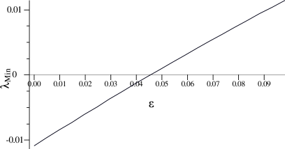
Figure 5: Application of Osaka’s map $\Phi_{O}$ on the convex combination $\rho^{\prime}\left(\varepsilon,\frac{5}{2}\right)=\frac{\varepsilon}{9}\mathbb{I}_{9}+(1-\varepsilon)\rho\left(\frac{5}{2}\right)$. $\varepsilon$ is plotted along the horizontal axis, and eigenvalues along the vertical axis. The line shows the minimum eigenvalue as a function of the robustness parameter $\varepsilon$. The state remains entangled approximately up to $\varepsilon=0.045$.

We now use the same procedure for $\rho(x,t)$ of the example in (10). The family of states is given by;

$$\rho^{\prime}(\varepsilon,x,t)=\frac{\varepsilon}{9}\mathbb{I}_{9}+(1-\varepsilon)\rho(x,t).$$

We use $\rho\left(\frac{7}{10},\frac{3}{40}\right)$, which is an entangled state and its entanglement is revealed by $\Phi\left(1+\frac{6}{10},1,1\right)$. Now the family $\rho^{\prime}\left(\varepsilon,\frac{7}{10},\frac{3}{40}\right)$ is dependent on $\varepsilon$. We plot the minimum eigenvalue of this family as a function of the robustness parameter $\varepsilon$. Figure 6 shows that up to approximately $\varepsilon=0.012$ the state remains entangled.

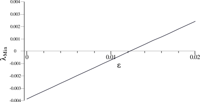
Figure 6: Application of $\Phi\left(1+\frac{6}{10},1,1\right)$ on $\rho^{\prime}\left(\varepsilon,\frac{7}{10},\frac{3}{40}\right)$. $\varepsilon$ is plotted along the horizontal axis, and eigenvalues along the vertical axis. The line shows the minimum eigenvalue as a function of the robustness parameter $\varepsilon$. The state remains entangled upto approximately $\varepsilon=0.012$.

IV Conclusions

This work is an exploration in the context of finding bound entangled states whose entanglement is revealed by witnesses based on positive maps that are not completely positive. We have managed to extend the construction to a class of bound entangled states using the Cholesky decomposition whose entanglement is revealed by Osaka’s map acting as a witness. Furthermore, we have generated a family of extremal extensions of Choi’s original map and shown that these extremal extensions are capable of revealing the entanglement of new classes of entangled states. We are extending this work to develop a more general framework where extremal movement in the map space is tracked down to a similar movement in the space of bound entangled states. Those results will be presented elsewhere.

References

- (1)
- Nielsen and Chuang (2000) M. A. Nielsen and I. L. Chuang, Quantum computation and quantum information (Cambridge University Press, Cambridge, 2000) .
- Horodecki et al. (1996) M. Horodecki, P. Horodecki, and R. Horodecki, Phys. Lett. A 223, 1 (1996).
- Peres (1996) A. Peres, Phys. Rev. Lett. 77, 1413 (1996).
- Woronowicz (1976a) S. L. Woronowicz, Rep. Math. Phys. 10, 165 (1976a).
- Arveson (1969) W. Arveson, Acta Math. 123, 141 (1969).
- Arveson (1974) W. Arveson, Ann. of Math. (2) 100, 433 (1974).
- Størmer (1963) E. Størmer, Acta Math. 110, 233 (1963).
- Størmer (1982) E. Størmer, Proc. Amer. Math. Soc. 86, 402 (1982).
- Jamiołkowski (1972) A. Jamiołkowski, Rep. Mathematical Phys. 3, 275 (1972).
- Woronowicz (1976b) S. L. Woronowicz, Comm. Math. Phys. 51, 243 (1976b).
- Horodecki et al. (2009) R. Horodecki, P. Horodecki, M. Horodecki, and K. Horodecki, Rev. Mod. Phys. 81, 865 (2009).
- Gühne and Tóth (2009) O. Gühne and G. Tóth, Phys. Rep. 474, 1 (2009).
- Choi (1975a) M. D. Choi, Linear Algebra and Appl. 12, 95 (1975a).
- Cho et al. (1992) S. J. Cho, S.-H. Kye, and S. G. Lee, Linear Algebra Appl. 171, 213 (1992).
- Ha (1998) K.-C. Ha, Publ. Res. Inst. Math. Sci. 34, 591 (1998).
- Osaka (1992) H. Osaka, Publ. Res. Inst. Math. Sci. 28, 747 (1992).
- Ha (2002) K.-C. Ha, Linear Algebra Appl. 348, 105 (2002).
- Terhal (2001) B. M. Terhal, Linear Algebra Appl. 323, 61 (2001).
- Robertson (1983a) A. G. Robertson, Quart. J. Math. Oxford Ser. (2) 34, 87 (1983a).
- Robertson (1983b) A. G. Robertson, Proc. Roy. Soc. Edinburgh Sect. A 94, 71 (1983b).
- Robertson (1983c) A. G. Robertson, Math. Proc. Cambridge Philos. Soc. 94, 291 (1983c).
- Robertson (1985) A. G. Robertson, J. London Math. Soc. (2) 32, 133 (1985).
- Kossakowski (2003) A. Kossakowski, Open Syst. Inf. Dyn. 10, 213 (2003).
- Kimura and Kossakowski (2004) G. Kimura and A. Kossakowski, Open Syst. Inf. Dyn. 11, 343 (2004).
- Chruściński and Kossakowski (2007) D. Chruściński and A. Kossakowski, Open Syst. Inf. Dyn. 14, 275 (2007).
- Choi and Lam (7778) M. D. Choi and T. Y. Lam, Math. Ann. 231, 1 (1977/78).
- Chruściński et al. (2008) D. Chruściński, J. Jurkowski, and A. Kossakowski, Phys. Rev. A 77, 022113 (2008).
- Rudin (2000) W. Rudin, Amer. Math. Monthly 107, 813 (2000).
- Ha (2003) K.-C. Ha, Linear Algebra Appl. 359, 277 (2003).
- Choi (1980) M. D. Choi, J. Operator Theory 4, 271 (1980).
- Bhatia (2007) R. Bhatia, Positive definite matrices, Princeton Series in Applied Mathematics (Princeton University Press, Princeton, NJ, 2007).
- Choi (1975b) M. D. Choi, Linear Algebra and Appl. 10, 285 (1975b).
- Chruściński and Kossakowski (2008) D. Chruściński and A. Kossakowski, J. Phys. A 41, 145301 (2008).