Analogs of noninteger powers in general analytic QCD

Abstract

In contrast to the coupling parameter in the usual perturbative QCD (pQCD), the coupling parameter in the analytic QCD models has cuts only on the negative semiaxis of the $Q^{2}$-plane (where $q^{2}\equiv-Q^{2}$ is the momentum squared), thus reflecting correctly the analytic structure of the spacelike observables. The Minimal Analytic model (MA, named also APT) of Shirkov and Solovtsov removes the nonphysical cut (at positive $Q^{2}$) of the usual pQCD coupling and keeps the pQCD cut discontinuity of the coupling at negative $Q^{2}$ unchanged. In order to evaluate in MA the physical QCD quantities whose perturbation expansion involves noninteger powers of the pQCD coupling, a specific method of construction of MA analogs of noninteger pQCD powers was developed by Bakulev, Mikhailov and Stefanis (BMS). We present a construction, applicable now in any analytic QCD model, of analytic analogs of noninteger pQCD powers; this method generalizes the BMS approach obtained in the framework of MA. We need to know only the discontinuity function of the analytic coupling (the analog of the pQCD coupling) along its cut in order to obtain the analytic analogs of the noninteger powers of the pQCD coupling, as well as their timelike (Minkowskian) counterparts. As an illustration, we apply the method to the evaluation of the width for the Higgs decay into $b{\bar{b}}$ pair.

I Introduction

It is well known that the perturbative approach to QCD (pQCD), while working well in evaluation of physical quantities at high momentum transfer ($|q^{2}|\gtrsim 10^{1}\ {\rm GeV}^{2}$), becomes increasingly unreliable at low momenta ($|q^{2}|\sim 1\ {\rm GeV}^{2}$). One of the main reasons for this is the singularity structure of the pQCD coupling parameter $a_{\rm pt}(Q^{2})\equiv\alpha_{s}(Q^{2})/\pi$ at spacelike low momenta $q$: $(0<)$ $Q^{2}\equiv-q^{2}\sim 1\ {\rm GeV}^{2}$. This singularity structure does not reflect correctly the analyticity structure of the (to be evaluated) spacelike observables ${\cal F}(Q^{2})$. The latter, by the general principles of the (local) quantum field theory BS ; Oehme , must be analytic functions in the entire $Q^{2}$ plane except on the cut on the negative semiaxis: $Q^{2}\in\mathbb{C}\backslash(-\infty,0]$. Qualitatively the same analytic properties should have also the coupling parameter ${\mathcal{A}}_{1}(Q^{2})$ that is used (instead of $a_{\rm pt}(Q^{2})$) to evaluate the spacelike observables ${\cal F}(Q^{2})$.

The first such analytic version was constructed in ShS ; MSS ; Sh , where the discontinuity function of pQCD $\rho_{1}^{\rm(pt)}(\sigma)={\rm Im}a_{\rm pt}(Q^{2}=-\sigma-i\epsilon)$ was kept unchanged on the entire negative axis in the $Q^{2}$-plane. More specifically, the use of the Cauchy theorem for the (powers of the) pQCD coupling gives

$$a^{n}_{\rm pt}(Q^{2})=\frac{1}{\pi}\int_{\sigma=-\Lambda_{\rm L}^{2}-\eta}^{\infty}\frac{d\sigma\ {\rm Im}a^{n}_{\rm pt}(-\sigma-i\epsilon)}{(\sigma+Q^{2})},$$ (1)

where the integration is along the entire cut of the pQCD coupling in the $Q^{2}$-plane $(-\infty,+\Lambda_{\rm L}^{2})$, with $0<\Lambda_{\rm L}^{2}\sim 1\ {\rm GeV}^{2}$ being the (Landau) branching point, and $\eta\to+0$ (see fig. 1).

Figure 1: The path of integration for the integral (1).

Elimination of the unphysical (Landau) cut $(0,+\Lambda_{\rm L}^{2})$ in the above dispersion relation leads to the aforementioned Minimal Analytic (MA) coupling

$${{{\mathcal{A}}_{n}^{\rm{(MA)}}}}(Q^{2})=\frac{1}{\pi}\int_{\sigma=0}^{\infty}\frac{d\sigma\ {\rm Im}{a^{n}_{\rm pt}(-\sigma-i\epsilon)}}{(\sigma+Q^{2})}\quad(n=1,2,\ldots).$$ (2)

It is named also Analytic Perturbation Theory (APT), ShS ; MSS ; Sh . It is applied usually in the ${\overline{\rm MS}}$ renormalization scheme, or in truncated versions of that scheme. The method of equation (2) allows us to evaluate the MA coupling analogs ${\mathcal{A}}_{n}^{\rm(MA)}(Q^{2})$ of the pQCD coupling powers $a_{\rm pt}^{n}(Q^{2})$ even when $n$ is noninteger $(n\mapsto\nu$).

MA gets its only free parameter, the QCD scale ${\overline{\Lambda}}$, fixed by the requirement that it reproduce high energy QCD quantities ($|Q^{2}|\stackrel{{\scriptstyle>}}{{\sim}}10^{1}\ {\rm GeV}^{2}$), and in this regime it gives good results, Sh . It gives good results for the Bjorken polarized sum rule (a spacelike quantity) even at low $Q^{2}$, BjPSR ; Bjnew , although at very low $Q^{2}\approx 0.1\ {\rm GeV}^{2}$ it apparently requires a modification Bjnew . Also due to duality violations we should expect that, at low $\sigma\sim 1\ {\rm GeV}^{2}$, the discontinuity function $\rho_{1}(\sigma)\equiv{\rm Im}{\mathcal{A}}_{1}(-\sigma-i\epsilon)$ in analytic QCD models will deviate significantly from the pQCD counterpart $\rho_{1}^{\rm(pt)}(\sigma)\equiv{\rm Im}a_{\rm pt}(-\sigma-i\epsilon)$. Another reason for the need of such a deviation is the apparent inability of MA to reproduce the correct value of the well-measured (timelike) low-energy QCD observable $r_{\tau}$, the strangeless semihadronic decay ratio of the $\tau$ lepton. Its present-day experimental value is $r_{\tau}({\rm exp.})=0.203\pm 0.004$, ALEPH ; DDHMZ . In MA, the predicted values are in the range of $0.13$-$0.14$, MSS ; MSSY , unless the values of the current masses of the light quarks ($m_{u}$, $m_{d}$, $m_{s}$) are abandoned and effective quark masses $\approx 0.25$-$0.45$ GeV are used instead Milton:2001mq . This numerical loss in the size of $r_{\tau}$ in MA appears to be connected with the elimination of the unphysical (Euclidean) part of the branch cut contribution of perturbative QCD, while keeping the discontinuity along the rest of the cut unchanged Geshkenbein:2001mn . Furthermore, perturbative QCD models which are simultaneously also analytic (anpQCD), have also been investigated, CKV , and they turn out to give too low $r_{\tau}$ value ($r_{\tau}<0.16$) unless their beta-function is modified in such a manner as to give convergence only in the first four terms of expansion, followed by explosive growth in the subsequent terms due to a rather singular choice of the renormalization scheme.

Therefore, in general analytic QCD models, we must expect the following form of the dispersion relation:

$${\mathcal{A}}_{1}(Q^{2})=\frac{1}{\pi}\int_{M_{\rm thr}^{2}}^{+\infty}\ d\sigma\frac{\rho_{1}(\sigma)}{(\sigma+Q^{2})}\ ,$$ (3)

with $\rho_{1}(\sigma)\equiv{\rm Im}{\mathcal{A}}_{1}(-\sigma-i\epsilon)$ deviating from $\rho_{1}^{\rm(pt)}(\sigma)$ at low $\sigma$, and $(0<)$ $M_{\rm thr}^{2}\sim M_{\pi}^{2}$ being a threshold mass of the cut $(-\infty,-M_{\rm thr}^{2})$ of ${\mathcal{A}}_{1}(q^{2})$ in the $Q^{2}$-plane. Having in such general analytic QCD models no direct relation of $a_{\rm pt}(Q^{2})$ with $\rho_{1}(\sigma)$, the general method of obtaining ${\mathcal{A}}_{n}(Q^{2})$, the analytic analog of the power $a_{\rm pt}(Q^{2})^{n}$, is not as straightforward as in equation (2) in the case of MA. In CV1 ; CV2 , the higher power analogs ${\mathcal{A}}_{n}(Q^{2})$ for integer $n$’s and for any analytic QCD were constructed as linear combinations of logarithmic derivatives ${\widetilde{\mathcal{A}}}_{k}(Q^{2})\propto d^{k-1}{\mathcal{A}}_{1}(Q^{2})/d(\ln Q^{2})^{k-1}$ ($k\geq n$), such that the evaluation of observables in analytic QCD leads to suppressed dependence of the evaluated truncated analytic series when the number of the terms in the series is increased. For the construction of ${\widetilde{\mathcal{A}}}_{n}(Q^{2})$ (and its timelike conterpart ${\widetilde{\mathfrak{A}}}_{n}(\sigma)$), only the knowledge of $\rho_{1}(\sigma)$ (or equivalently, of ${\mathcal{A}}_{1}(Q^{2})$) is needed. The construction of higher power analogs ${\mathcal{A}}_{n}$, not as powers of ${\mathcal{A}}_{1}$ but rather as linear operations on ${\mathcal{A}}_{1}$, has an attractive functional feature: it is compatible with linear integral transformations (such as Fourier or Laplace) Shirkov:1999np .

It turns out that some observables, in particular mass-dependent ones, have pQCD expansion which involves noninteger powers $a_{\rm pt}(Q^{2})^{\nu}$. In order to evaluate such observables in any analytic QCD, we need to construct their analytic analogs $A_{\nu}(Q^{2})$ (and their timelike conterparts ${\mathfrak{A}}_{\nu}(\sigma)$). In the case of MA, a method of calculating such quantities was developed and applied in BMS1 ; BMS2 ; BMS3 ; BP (for a review, see Bakulev ), their method being different from the direct evaluation (2) with $n\mapsto\nu$ ($\nu$ noninteger). The analytic properties of their couplings ${\mathcal{A}}_{\nu}^{\rm(MA)}(Q^{2})$ can be seen more clearly than in the formulas (2), but numerically they are equivalent. In the present paper, we present the method of construction of ${\mathcal{A}}_{\nu}(Q^{2})$’s that is applicable in any analytic QCD model. Below we will demonstrate that, within the MA model of Shirkov and Solovtsov, our approach gives the same result as the approach of BMS1 ; BMS2 ; BMS3 in the leading (one-loop) order of perturbation theory. Above the leading order in MA, the results of BMS1 ; BMS2 ; BMS3 are represented as certain expansions via the leading order results. Such types of expansions are absent in our approach.

In sections II and III we derive the spacelike analogs ${\mathcal{A}}_{\nu}(Q^{2})$ of noninteger pQCD powers $a_{\rm pt}(Q^{2})^{\nu}$, as functions of $\rho_{1}(\sigma)$ of the analytic QCD model. In sec. II, the construction leads us first to (noninteger counterparts) of the logarithmic derivatives, ${\widetilde{a}}_{{\rm pt},\nu}(Q^{2})$, and their analytic analogs ${\widetilde{\mathcal{A}}}_{\nu}(Q^{2})$. In sec. III we relate ${\widetilde{a}}_{{\rm pt},\nu}(Q^{2})$ with the pQCD (noninteger) powers $a_{\rm pt}(Q^{2})^{\nu+m}$; this relation is derived in appendix A. This allows us to evaluate the mentioned spacelike observables ${\cal F}(Q^{2})$ in analytic QCD using either the analytic analogs ${\widetilde{\mathcal{A}}}_{\nu}(Q^{2})$ of ${\widetilde{a}}_{{\rm pt},\nu}(Q^{2})$, or the analytic analogs ${\mathcal{A}}_{\nu}(Q^{2})$ of $a_{\rm pt}(Q^{2})^{\nu}$. Furthermore, we construct the timelike counterparts ${\widetilde{\mathfrak{A}}}_{\nu}(\sigma)$ and ${\mathfrak{A}}_{\nu}(\sigma)$ of the spacelike couplings ${\widetilde{\mathcal{A}}}_{\nu}(Q^{2})$ and ${\mathcal{A}}_{\nu}(Q^{2})$. In sec. IV we apply, as an illustration, the presented method to evaluation of a timelike quantity, the width of the Higgs decay into $b{\bar{b}}$ pair, $\Gamma(H\to b{\bar{b}})$. The corresponding spacelike quantity has a perturbation expansion which involves noninteger powers of $a_{\rm pt}$, due to the $b$-quark mass anomalous dimension. We present the results for $\Gamma(H\to b{\bar{b}})$ as a function of the squared Higgs mass $s=M_{H}^{2}$, for various analytic QCD scenarios and in pQCD. In sec. V we present conclusions.

II Logarithmic noninteger derivatives of Euclidean coupling in any analytic QCD model

As mentioned in the Introduction, we will start with the analytic Euclidean coupling ${\mathcal{A}}_{1}(Q^{2})$ and its logarithmic derivatives in a general analytic QCD model. Such a model is determined (characterized) fully by the discontinuity function

$$\rho_{1}(\sigma)={\rm Im}\ {\mathcal{A}}_{1}(Q^{2}=-\sigma-i\varepsilon)\ ,$$ (4)

defined for $\sigma\geq 0$. Usually, the discontinuity cut is nonzero below a threshold value $-\sigma\leq-M_{\rm thr}^{2}$ where $M_{\rm thr}\sim M_{\pi}$. The application of the Cauchy theorem to the function ${\mathcal{A}}_{1}(Q^{{}^{\prime}2})/(Q^{{}^{\prime}2}-Q^{2})$ in the complex $Q^{{}^{\prime}2}$-plane, along the closed path made of a very large circle and two segments just below and above the cut, gives us the well known dispersion relation for the analytic Euclidean coupling ${\mathcal{A}}_{1}$

$${\mathcal{A}}_{1}(Q^{2})=\frac{1}{\pi}\int_{0}^{+\infty}\ d\sigma\frac{\rho_{1}(\sigma)}{(\sigma+Q^{2})}\ ,$$ (5)

where $q^{2}\equiv-Q^{2}$ is non-Minkowskian, i.e., $Q^{2}$ can have any value in the complex plane except the cut $(-\infty,-M^{2}_{\rm thr}]$. The logarithmic derivatives are defined as

$${\widetilde{\mathcal{A}}}_{n+1}(Q^{2})\equiv\frac{(-1)^{n}}{\beta_{0}^{n}n!}\frac{\partial^{n}{\mathcal{A}}_{1}(Q^{2})}{\partial(\ln Q^{2})^{n}}\ ,\qquad(n=0,1,2,\ldots)\ ,$$ (6)

where $\beta_{0}$ is the first coefficient of the $\beta$ function: $\beta_{0}=(1/4)(11-2n_{f}/3)$; $Q^{2}da_{\rm pt}/dQ^{2}=-\beta_{0}a_{\rm pt}^{2}+{\cal O}(a_{\rm pt}^{3})$. We note that for $n=0$ equation (6) gives ${\widetilde{\mathcal{A}}}_{1}\equiv{\mathcal{A}}_{1}$. We can write the logarithmic derivatives in the following form:

$${\widetilde{\mathcal{A}}}_{n+1}(Q^{2})=\frac{1}{\pi}\int_{0}^{\infty}\ \frac{d\sigma}{\sigma}\rho_{1}(\sigma)\frac{1}{\beta_{0}^{n}\Gamma(n+1)}\frac{d^{n}}{d(\ln z)^{n}}\left(\frac{z}{1+z}\right){\Big{|}}_{z=\sigma/Q^{2}}\ .$$ (7)

It turns out that the integrand is the known polylogarithm function

$$\frac{d^{n}}{d(\ln z)^{n}}\left(\frac{z}{1+z}\right)=\left(z\frac{d}{dz}\right)^{n}\,\sum_{m=1}^{\infty}(-1)^{m+1}z^{m}=\sum_{m=1}^{\infty}(-1)^{m+1}m^{n}z^{m}=(-1){\rm Li}_{-n}(-z)\ ,$$ (8)

which brings equation (7) in the following form:

$${\widetilde{\mathcal{A}}}_{n+1}(Q^{2})=\frac{1}{\pi}\frac{(-1)}{\beta_{0}^{n}\Gamma(n+1)}\int_{0}^{\infty}\ \frac{d\sigma}{\sigma}\rho_{1}(\sigma){\rm Li}_{-n}(-\sigma/Q^{2})\ .$$ (9)

This relation is valid for $n=0,1,2,...$. Analytic continuation in $n\mapsto\nu$ gives us the logarithmic noninteger derivatives

$${\widetilde{\mathcal{A}}}_{\nu+1}(Q^{2})=\frac{1}{\pi}\frac{(-1)}{\beta_{0}^{\nu}\Gamma(\nu+1)}\int_{0}^{\infty}\ \frac{d\sigma}{\sigma}\rho_{1}(\sigma){\rm Li}_{-\nu}\left(-\frac{\sigma}{Q^{2}}\right)\quad(-1<\nu)\ .$$ (10)

We note that the integral converges for $\nu>-1$. Namely, at high $\sigma$ ($|z|\gg 1$ where $z\equiv\sigma/Q^{2}$) we have in the integrand of equation (10): $\rho_{1}(\sigma)\approx\rho_{1}^{\rm(pt)}(\sigma)\sim\ln^{-2}\sigma\sim\ln^{-2}z$ and ${\rm Li}_{-\nu}(-z)\sim\ln^{-\nu}z$ (for noninteger $\nu$). Therefore, the integral converges at $\sigma\to\infty$ if $\nu>-1$. The integral obviously converges at low $\sigma$, too.

In principle, a continuation to arbitrary $\nu$, as performed by the transition from equation (9) to equation (10), could in principle miss some terms, such as terms proportional to $\sin^{k}(\nu\pi)$. However, such terms will be excluded because they are finite oscillatory when $\nu\to\pm\infty$.

It is interesting that the recursive relation

$${\widetilde{\mathcal{A}}}_{\nu+2}(Q^{2})=\frac{(-1)}{\beta_{0}(\nu+1)}\frac{d}{d\ln Q^{2}}{{\widetilde{\mathcal{A}}}}_{\nu+1}(Q^{2})\ ,$$ (11)

which for positive integer $\nu=n=0,1,2,\ldots$ is a direct consequence of the definition (7), remains valid even for noninteger $\nu$ as a consequence of the relation (10) and the known relation $z(d/dz){\rm Li}_{-\nu}(z)={\rm Li}_{-\nu-1}(z)$.

We can recast the result (10) into an alternative form involving the spacelike coupling ${\mathcal{A}}_{1}$ instead of the discontinuity function $\rho_{1}(\sigma)$. This can be performed in the following way.

We can use the following integral form of ${\rm Li}_{-\nu}$ function (PBM ) appearing in equation (10):

$${\rm Li}_{-\nu}(z)=\frac{z}{\Gamma(-\nu)}\int_{0}^{\infty}\frac{dt\;t^{-\nu-1}}{(e^{t}-z)}=\frac{z}{\Gamma(-\nu)}\int_{0}^{1}\frac{d\xi}{1-z\xi}\ln^{-\nu-1}\left(\frac{1}{\xi}\right)\quad(\nu<0)\ .$$ (12)

The last expression on the right-hand side was obtained by the change of variable $t=\ln(1/\xi)$. Since we have in our result (10) ${\rm Li}_{-\nu}$ with $-1<\nu$ (and not just: $-1<\nu<0$), we extend the integral representation to higher $\nu>0$. This is achieved by using in equation (12) the aforementioned relation $(d/d\ln z){\rm Li}_{-\nu}={\rm Li}_{-\nu-1}$. We thus obtain, for $\nu=n+\delta$, with $0<\delta<1$ and $n=-1,0,1,2,\ldots$, the following integral form, Kotikov:2010bm :

$${\rm Li}_{-n-\delta}(z)=\left(\frac{d}{d\ln z}\right)^{n+1}\left[\frac{z}{\Gamma(1-\delta)}\int_{0}^{1}\frac{d\xi}{1-z\xi}\ln^{-\delta}\left(\frac{1}{\xi}\right)\right]\quad(n=-1,0,1,\ldots;\ 0<\delta<1)\ .$$ (13)

Inserting the representation (13), for $\nu=n+\delta$, into our general formula (10), and exchanging the order of integration, gives us

$${\widetilde{\mathcal{A}}}_{\nu+1}(Q^{2}) = \frac{1}{\beta_{0}^{\nu}\Gamma(n+1+\delta)\Gamma(1-\delta)}\left(-\frac{d}{d\ln Q^{2}}\right)^{n+1}\int_{0}^{1}\frac{d\xi}{\xi}\ln^{-\delta}\left(\frac{1}{\xi}\right)\int_{0}^{\infty}\frac{d\sigma\rho_{1}(\sigma)}{\pi(\sigma+Q^{2}/\xi)}\ .$$ (14)

The last integral over $d\sigma$ is the spacelike coupling ${\mathcal{A}}_{1}(Q^{2}/\xi)$ due to the dispersion relation (5). Therefore, we obtain the alternative form of the result (10), for $\nu=n+\delta$, with $0<\delta<1$ and $n=-1,0,1,2,\ldots$,

$${\widetilde{\mathcal{A}}}_{\nu+1}(Q^{2})\equiv{\widetilde{\mathcal{A}}}_{n+1+\delta}(Q^{2}) = \frac{1}{\beta_{0}^{\nu}\Gamma(1+\nu)\Gamma(1-\delta)}\left(-\frac{d}{d\ln Q^{2}}\right)^{n+1}\int_{0}^{1}\frac{d\xi}{\xi}{\mathcal{A}}_{1}(Q^{2}/\xi)\ln^{-\delta}\left(\frac{1}{\xi}\right)$$ (15)

$$= \frac{1}{\beta_{0}^{\nu}}\frac{\Gamma(1+\delta)}{\Gamma(n+1+\delta)}\frac{\sin(\pi\delta)}{(\pi\delta)}\left(-\frac{d}{d\ln Q^{2}}\right)^{n+1}\int_{0}^{\infty}\frac{dt}{t^{\delta}}{\mathcal{A}}_{1}(Q^{2}e^{t})\ ,$$ (16)

where the last form (16) was obtained from the previous one by the substitution $t=\ln(1/\xi)$ and using the identity $\Gamma(1+\delta)\Gamma(1-\delta)=\pi\delta/\sin(\pi\delta)$.

Furthermore, we will now prove that the obtained result (10) (equivalent to equations (15) and (16)) reproduces, in the specific case of the Minimal Analytic model (MA) of ShS ; MSS ; Sh at one-loop level, the explicit result obtained in BMS1

$${\widetilde{\mathcal{A}}}_{\nu+1}(Q^{2})^{\rm(MA,1-\ell)}={\mathcal{A}}_{\nu+1}(Q^{2})^{\rm(MA,1-\ell)}=\frac{1}{\beta_{0}^{\nu+1}}\left(\frac{1}{\ln^{\nu+1}(Q^{2}/\overline{\Lambda}^{2})}-\frac{{\rm Li}_{-\nu}(\overline{\Lambda}^{2}/Q^{2})}{\Gamma(\nu+1)}\right)\ ,$$ (17)

where the scale $\overline{\Lambda}$ appears in the one-loop MA analytic coupling ${\mathcal{A}}_{1}(Q^{2})^{\rm(MA,1-\ell)}$ and in its discontinuity function $\rho_{1}(\sigma)_{\rm pt}^{\rm(1-\ell)}$

$${\mathcal{A}}_{1}(Q^{2})^{\rm(MA,1-\ell)} = \frac{1}{\beta_{0}}\left(\frac{1}{\ln(Q^{2}/\overline{\Lambda}^{2})}-\frac{\overline{\Lambda}^{2}}{(Q^{2}-\overline{\Lambda}^{2})}\right)\ ,$$ (18)

$$\rho_{1}(\sigma)_{\rm pt}^{\rm(1-\ell)} = {\rm Im}a_{\rm pt}(-\sigma-i\epsilon)^{\rm(1-\ell)}={\rm Im}{\mathcal{A}}_{1}(-\sigma-i\epsilon)^{\rm(MA,1-\ell)}$$ (19)

$$= \frac{1}{\beta_{0}}{\rm Im}\frac{1}{\left(\ln(\sigma/\overline{\Lambda})-i\pi\right)}=\frac{\pi}{\beta_{0}}\frac{1}{\left(\ln^{2}(\sigma/\overline{\Lambda})+\pi^{2}\right)}\ .$$

When replacing ${\mathcal{A}}_{1}(Q^{2}/\xi)$ in the integrand of the expression (15) by the second term of the expression (18) for ${\mathcal{A}}_{1}(Q^{2}/\xi)^{\rm(MA,1-\ell)}$, and using the integral form (13) for ${\rm Li}_{-\nu}$, we obtain immediately

$$\frac{1}{\beta_{0}^{\nu}\Gamma(1+\nu)\Gamma(1-\delta)}\left(-\frac{d}{d\ln Q^{2}}\right)^{n+1}\int_{0}^{1}\frac{d\xi}{\xi}\ln^{-\delta}\left(\frac{1}{\xi}\right)\frac{1}{\beta_{0}}\frac{(-1)\overline{\Lambda}^{2}}{(Q^{2}/\xi-\overline{\Lambda}^{2})} = \frac{(-1)}{\beta_{0}^{\nu+1}\Gamma(\nu+1)}{\rm Li}_{-\nu}(\overline{\Lambda}^{2}/Q^{2})\ .$$ (20)

On the other hand, when replacing ${\mathcal{A}}_{1}(Q^{2}/\xi)$ in the integrand of the expression (16) by the first term of the expression (18) for ${\mathcal{A}}_{1}(Q^{2}/\xi)^{\rm(MA,1-\ell)}$, we obtain in a direct manner

$$\frac{1}{\beta_{0}^{\nu}}\frac{\Gamma(1+\delta)}{\Gamma(n+1+\delta)}\frac{\sin(\pi\delta)}{(\pi\delta)}\left(-\frac{d}{d\ln Q^{2}}\right)^{n+1}\int_{0}^{\infty}\frac{dt}{t^{\delta}}\frac{1}{\beta_{0}}\frac{1}{\left[t+\ln(Q^{2}/\overline{\Lambda}^{2})\right]} = \frac{1}{\beta_{0}^{\nu+1}\ln^{\nu+1}(Q^{2}/\overline{\Lambda}^{2})}\ .$$ (21)

Combining the results (20) and (21), we obtain the full result (17) for ${\mathcal{A}}_{\nu+1}(Q^{2})$ in the one-loop approach of MA, for any noninteger $\nu$ such that $-1<\nu$ (when $\nu$ is nonnegative integer, the limit $\delta\to 0$ can be made in the derivation). This (one-loop MA) result, obtained for the first time by Bakulev, Mikhailov and Stefanis (BMS) in BMS1 , has several interesting properties, as pointed out in BMS2 (their equations (3.14)-(3.19)). The result (17) is explicit and allows us to apply it even for $\nu\leq-1$, and even for complex $\nu$; this is a kind of analytic continuation in $\nu$. We can thus use this result, by adding and subtracting it from of our general integral expression (10), thus extending the $\nu$-regime of applicability of our expression

$${\widetilde{\mathcal{A}}}_{\nu+1}(Q^{2}) = {\widetilde{\mathcal{A}}}_{\nu+1}(Q^{2})^{\rm(MA,1-\ell)}+\frac{1}{\pi}\frac{(-1)}{\beta_{0}^{\nu}\Gamma(\nu+1)}\int_{0}^{\infty}\ \frac{d\sigma}{\sigma}\left[\rho_{1}(\sigma)-\rho_{1}(\sigma)_{\rm pt}^{\rm(1-\ell)}\right]{\rm Li}_{-\nu}\left(-\frac{\sigma}{Q^{2}}\right)\quad(-2<\nu)\ ,$$ (22)

where ${\widetilde{\mathcal{A}}}_{\nu+1}(Q^{2})^{\rm(MA,1-\ell)}$ and $\rho_{1}(\sigma)_{\rm pt}^{\rm(1-\ell)}$ are given in equations (17) and (19), respectively. Now the integral converges also for $-2<\nu<-1$, because, due to asymptotic freedom, the difference $[\rho_{1}(\sigma)-\rho_{1}(\sigma)_{\rm pt}^{\rm(1-\ell)}]$ behaves at large $\sigma$ as $\sim\ln\ln\sigma/\ln^{3}\sigma$ and not as $1/\ln^{2}\sigma$. Further, the expression (22) implies that ${\widetilde{\mathcal{A}}}_{0}(Q^{2})$ [$\equiv{\rm lim}_{\nu\to-1}{\widetilde{\mathcal{A}}}_{\nu+1}(Q^{2})$] $=1$ for all complex $Q^{2}$, because: ${\rm Li}_{-\nu}(z)/\Gamma(\nu+1)\to 0$ when $\nu\to-1$, and ${\widetilde{\mathcal{A}}}_{0}(Q^{2})^{\rm(MA,1-\ell)}\equiv 1$.

III Analytization procedure for observables with noninteger powers of coupling

In QCD we encounter often spacelike (Euclidean) observables ${\cal F}(Q^{2})$ whose perturbative expansion starts with a noninteger power $a_{\rm pt}^{\nu_{0}}$

$${\cal F}(Q^{2})_{\rm pt}=a_{\rm pt}(Q^{2})^{\nu_{0}}+{\cal F}_{1}a_{\rm pt}(Q^{2})^{\nu_{0}+1}+{\cal F}_{2}a_{\rm pt}(Q^{2})^{\nu_{0}+2}+\cdots$$ (23)

The general analytization procedure of the pQCD-evaluated observables with integer powers is

$${{\widetilde{a}}}_{{\rm pt},n+1}\mapsto{\widetilde{\mathcal{A}}}_{n+1}\quad(n=0,1,2,\ldots)\ ,$$ (24)

where ${{\widetilde{a}}}_{{\rm pt},n+1}$ are the logarithmic derivatives of the pQCD coupling $a_{\rm pt}$

$${{\widetilde{a}}}_{{\rm pt},n+1}(Q^{2})\equiv\frac{(-1)^{n}}{\beta_{0}^{n}n!}\frac{\partial^{n}a_{\rm pt}(Q^{2})}{\partial(\ln Q^{2})^{n}}=a_{\rm pt}^{n}+{\cal O}(a_{\rm pt}^{n+1})\qquad(n=0,1,2,\ldots)\ ,$$ (25)

and $\beta_{0}$ is the first coefficient of the $\beta$-function

$$\frac{da_{\rm pt}(\mu^{2})}{d\ln\mu^{2}}\equiv\beta(a_{\rm pt}) = -\beta_{0}a_{\rm pt}^{2}-\beta_{1}a_{\rm pt}^{3}-\beta_{2}a_{\rm pt}^{4}-\beta_{3}a_{\rm pt}^{5}-\beta_{4}a_{\rm pt}^{6}-\dots$$ (26)

$$= -\beta_{0}a_{\rm pt}^{2}\,\left(1+c_{1}a_{\rm pt}+c_{2}a_{\rm pt}^{2}+c_{3}a_{\rm pt}^{3}+c_{4}a_{\rm pt}^{4}+\dots\right)~{}~{}~{}\left(c_{j}=\frac{\beta_{j}}{\beta_{0}}\right)\ .$$

In the case of observables whose pQCD-evaluated expressions are the (truncated) expansions equation (23) with noninteger $\nu_{0}$, the analytization procedure (24) is naturally extended to (CV1 ; CV2 )

$${{\widetilde{a}}}_{{\rm pt},\nu+1}\mapsto{\widetilde{\mathcal{A}}}_{\nu+1}\ ,$$ (27)

where the expression for ${\widetilde{\mathcal{A}}}_{\nu+1}$ is given in equation (10). Therefore, at this stage, the problem of evaluation of such observables in anQCD is reduced to re-expressing the noninteger powers $a_{\rm pt}^{\nu}$ in pQCD expansion (23) in terms of the logarithmic noninteger derivatives ${{\widetilde{a}}}_{{\rm pt},\nu+m}(Q^{2})$, in order to perform the subsequent analytization via equation (27). Stated otherwise, we find first the coefficients $k_{m}(\nu)$ of the relations

$${{\widetilde{a}}}_{{\rm pt},\nu}~{}=~{}a_{\rm pt}^{\nu}+\sum_{m=1}^{\infty}k_{m}(\nu)a_{\rm pt}^{\nu+m}\ ,$$ (28)

and, as a consequence, the coefficients ${\widetilde{k}}_{m}(\nu)$ of the inverse relations

$$a_{\rm pt}^{\nu}~{}=~{}{{\widetilde{a}}}_{{\rm pt},\nu}+\sum_{m=1}^{\infty}{\widetilde{k}}_{m}(\nu){{\widetilde{a}}}_{{\rm pt},\nu+m}\ .$$ (29)

The expressions for the coefficients $k_{m}(\nu)$ (and ${\widetilde{k}}_{m}(\nu)$) are derived in appendix A; see equations (83)-(86), (87) and (88) there for explicit expressions. There, the coefficients $k_{m}(n)$ and ${\widetilde{k}}_{m}(n)$, for $n$ integer, are obtained by solving the difference (recursion) equations relating $k_{m}(n+1)$ with $k_{m}(n)$, $k_{m-1}(n)$, etc. The solution for $k_{m}(n)$ (and ${\widetilde{k}}_{m}(n)$) is obtained in a form involving combinations of Gamma functions $\Gamma(x)$ and their derivatives (up to $m$ derivatives), at the values of the argument $x=1$ and $x=+n+m^{\prime}$ (for $m^{\prime}=1,\ldots,m$). In the obtained expressions, the integer $n$ is then replaced by an arbitrary noninteger $\nu$ ($n\mapsto\nu$). The latter step is an analytic continuation similar to the step $n\mapsto\nu$ from equation (9) to equation (10).

The relations (29) allow us to reexpress the expansion (23) in terms of ${{\widetilde{a}}}_{{\rm pt},\nu}$’s

$${\cal F}(Q^{2})_{\rm mpt}={{\widetilde{a}}}_{\rm pt,\nu_{0}}(Q^{2})+{\widetilde{\cal F}}_{1}{{\widetilde{a}}}_{\rm pt,\nu_{0}+1}(Q^{2})+{\widetilde{\cal F}}_{2}{{\widetilde{a}}}_{\rm pt,\nu_{0}+2}(Q^{2})+\cdots\ ,$$ (30)

where ’mpt’ stands for “modified perturbation series” and the coefficients ${\widetilde{\cal F}}_{n}$ are related with the coefficients ${\cal F}_{n}$ of the original perturbation series (23) via relations involving the coefficients ${\widetilde{k}}_{m}(\nu_{0}+n)$ appearing in the relations (29)

$${\widetilde{\cal F}}_{1}={\cal F}_{1}+{\widetilde{k}}_{1}(\nu_{0}),\quad{\widetilde{\cal F}}_{2}={\cal F}_{2}+{\cal F}_{1}{\widetilde{k}}_{1}(\nu_{0}+1)+{\widetilde{k}}_{2}(\nu_{0})\ ,\quad{\rm etc.}$$ (31)

See equations (99)-(102) in appendix A for more relations involving higher orders.

At this stage we apply the analytization procedure (27) to obtain the “modified analytic” (man) series for the (dimensionless) spacelike quantity ${\cal F}(Q^{2})$

$${\cal F}(Q^{2})_{\rm man}={{\widetilde{\mathcal{A}}}}_{\nu_{0}}(Q^{2})+{\widetilde{\cal F}}_{1}{{\widetilde{\mathcal{A}}}}_{\nu_{0}+1}(Q^{2})+{\widetilde{\cal F}}_{2}{{\widetilde{\mathcal{A}}}}_{\nu_{0}+2}(Q^{2})+\cdots\ ,$$ (32)

where the expressions for ${{\widetilde{\mathcal{A}}}}_{\nu_{0}+1}(Q^{2})$, ${{\widetilde{\mathcal{A}}}}_{\nu_{0}+2}(Q^{2})$ are given, in any given anQCD, by equation (10).

On the other hand, an observable ${\cal T}(\sigma)$ that is related with a spacelike observable ${\cal F}(Q^{2})$ via the integral transformation

$${\cal F}(Q^{2})=Q^{2}\int_{0}^{\infty}\frac{d\sigma\ {\cal T}(\sigma)}{(\sigma+Q^{2})^{2}}$$ (33)

is timelike (Minkowskian). The inverse transformation is

$${\cal T}(\sigma)=\frac{1}{2\pi i}\int_{-\sigma-i\varepsilon}^{-\sigma+i\varepsilon}\frac{dQ^{{}^{\prime}2}}{Q^{{}^{\prime}2}}{\cal F}(Q^{{}^{\prime}2})\ ,$$ (34)

where the integration contour is in the complex $Q^{{}^{\prime}2}$-plane encircling the singularities of the integrand, e.g., path ${\cal C}_{1}$ or ${\cal C}_{2}$ of fig. 2.

Figure 2: Paths ${\cal C}_{1}$ and ${\cal C}_{2}$ in the complex $Q^{{}^{\prime}2}$-plane.

Application of the tranformation (34) to the (modified) analytic series (32) then gives for the timelike quantity ${\cal T}(\sigma)$ the following (Minkowskian) “modified analytic series”

$${\cal T}(\sigma)_{\rm man}={{\widetilde{\mathfrak{A}}}}_{\nu_{0}}(\sigma)+{\widetilde{\cal F}}_{1}{{\widetilde{\mathfrak{A}}}}_{\nu_{0}+1}(\sigma)+{\widetilde{\cal F}}_{2}{{\widetilde{\mathfrak{A}}}}_{\nu_{0}+2}(\sigma)+\cdots\ ,$$ (35)

where the timelike (Minkowskian) couplings ${{\widetilde{\mathfrak{A}}}}_{\nu+1}(\sigma)$ are defined as

$${{\widetilde{\mathfrak{A}}}}_{\nu+1}(\sigma)\equiv\frac{1}{2\pi i}\int_{-\sigma-i\varepsilon}^{-\sigma+i\varepsilon}\frac{dQ^{{}^{\prime}2}}{Q^{{}^{\prime}2}}{{\widetilde{\mathcal{A}}}}_{\nu+1}(Q^{{}^{\prime}2})\ ,$$ (36)

and the inverse transformation is

$${\widetilde{\mathcal{A}}}_{\nu+1}(Q^{2})=Q^{2}\int_{0}^{\infty}\frac{d\sigma\;{{\widetilde{\mathfrak{A}}}}_{\nu+1}(\sigma)}{(\sigma+Q^{2})^{2}}\ .$$ (37)

Here we would like to note that the reexpression of the expansion (23) to the one of equation (30) is a well-defined operation for quite convergent series. It is well known that mostly the QCD series are assumed to be asymptotic (see, for example, Kazakov:1980rd ), and some arguments to justify such a reexpression should be done, despite the fact that we use in our analysis only the first several terms in the expansions (23) and (30). Some cases of different types of asymptotics were recently considered in Shirkov:2012zm .

To show the correctness of the reexpression and, at the same time, to avoid an additional increase of the volume of the main text part of our paper, we consider in appendix B the standard Lipatov-type behavior Lipatov:1976ny for the $n$th term of the expansion (23) and recover the similar behavior for the $n$th term of the expansion (30). We show that there is even a slight weakening of the rise for the $n$th term of the expansion (30) in comparison with the original one in the expansion (23) if the coefficients in (23) are nonalternating in sign.

The parameter ${{\widetilde{a}}}_{\rm pt,\nu_{0}+n}(Q^{2})$ of the expansion (30) is very close to the corresponding one $a_{\rm pt}^{\nu_{0}+n}(Q^{2})$ in the high-momentum regime (i.e., when $a_{\rm pt}$-values are small). This observation is consistent with the similarity of the coefficients ${\cal F}_{n}$ and ${\widetilde{\cal F}}_{n}$ shown in appendix B, and another argument for acceptability of the reexpression of the expansion (23) to the one of equation (30).

We note also that, after the analytization procedure (27), there is in general a significant supppression of the new parameters ${\widetilde{\mathcal{A}}}_{\nu_{0}+n}(Q^{2})$ in comparison with ${{\widetilde{a}}}_{\rm pt,\nu_{0}+n}(Q^{2})$ and $a_{\rm pt}^{\nu_{0}+n}(Q^{2})$ (see a recent review Bakulev and discussions therein).

III.1 Timelike (Minkowskian) coupling parameter

Direct use of the expression (10) in the integral (36) gives us a double integral. When $-1<\nu<1$, the order of integration can be exchanged because the resulting double integral is convergent, and we obtain

$${{\widetilde{\mathfrak{A}}}}_{\nu+1}(\sigma)=\frac{(-1)}{2\pi i\beta_{0}^{\nu}\Gamma(\nu+1)}\int_{0}^{\infty}\frac{d\sigma^{\prime}}{\sigma^{\prime}}\rho_{1}(\sigma^{\prime})\int_{-\sigma-i\varepsilon}^{-\sigma+i\varepsilon}\frac{dQ^{{}^{\prime}2}}{Q^{{}^{\prime}2}}{\rm Li}_{-\nu}(-\sigma^{\prime}/Q^{{}^{\prime}2})\ .$$ (38)

Now we can use the fact that ${\rm Li}_{-\nu}(z)$ is a function with a branch cut discontinuity $[1,+\infty)$ in the complex $z$-plane, and the earlier mentioned relation ${\rm Li}_{-\nu}(z)=d{\rm Li}_{1-\nu}(z)/d\ln z$, to obtain the identity

$$\frac{1}{2\pi i}\oint_{|z|=\kappa,{\rm pos.dir.}}\frac{dz}{z}{\rm Li}_{-\nu}(z)=\frac{1}{\pi}{\rm Im}{\rm Li}_{1-\nu}(\kappa-i\varepsilon)=-\frac{1}{\Gamma(1-\nu)}(\ln\kappa)^{-\nu}\Theta(\kappa-1)\ ,$$ (39)

where $\Theta$ on the right-hand side is the Heaviside step function, and the integration on the left-hand side is along the contour of radius $|z|=\kappa$ over the angles $\Phi\equiv{\rm arg}(z)$ from $+0$ to $(2\pi-0)$, see fig. 3.

Figure 3: Integration contour for the integral (39).

Using the relation (39) in the integration over $Q^{{}^{\prime}2}$ on the right-hand side of equation (38), we obtain the simplified expression for the general Minkowskian coupling ${{\widetilde{\mathfrak{A}}}}_{\nu+1}(\sigma)$ in any analytic QCD and for any real $\nu$ in the interval $-1<\nu<1$

$${{\widetilde{\mathfrak{A}}}}_{\nu+1}(\sigma)=\frac{\sin(\pi\nu)}{\pi^{2}\nu\beta_{0}^{\nu}}\int_{0}^{\infty}\frac{dw}{w^{\nu}}\rho_{1}(\sigma e^{w})\ ,\quad(-1<\nu<1)\ ,$$ (40)

and we used here a new variable $w=\ln(\sigma^{\prime}/\sigma)$. The integral (40) is clearly convergent at $w\to 0$. It is also convergent at $w\to+\infty$, because there $\rho_{1}(\sigma e^{w})\approx\rho_{1}^{\rm(pt)}(\sigma e^{w})\sim 1/w^{2}$.

The case of ${{\mathfrak{A}}}_{1}(\sigma)$ is obtained in the limit $\nu\to+0$ of the above expression

$${{\mathfrak{A}}}_{1}(\sigma)={{\widetilde{\mathfrak{A}}}}_{1}(\sigma)=\frac{1}{\pi}\int_{0}^{\infty}dw\ \rho_{1}(\sigma e^{w})=\frac{1}{\pi}\int_{\sigma}^{\infty}\frac{d\sigma^{\prime}}{\sigma^{\prime}}\rho_{1}(\sigma^{\prime})\ ,$$ (41)

which is a well known result. For Minkowskian couplings ${{\widetilde{\mathfrak{A}}}}_{\nu+1}={{\widetilde{\mathfrak{A}}}}_{\delta+1+n}(\sigma)$ with higher index $\nu=n+\delta$ ($n=0,1,2,\ldots$; and $0<\delta<1$), we can use the recursion formulas

$${{\widetilde{\mathfrak{A}}}}_{\nu+2}(\sigma)=\frac{(-1)}{\beta_{0}(\nu+1)}\frac{d}{d\ln\sigma}{{\widetilde{\mathfrak{A}}}}_{\nu+1}(\sigma)\ ,$$ (42)

which can be obtained from the relations (11) and (36), and obtain (see appendix C for derivation)

$${{\widetilde{\mathfrak{A}}}}_{\nu+1}(\sigma) = \frac{\sin(\pi(\delta+n))}{\pi^{2}(\delta+n)\beta_{0}^{\delta+n}}\int_{0}^{\infty}\frac{dw}{w^{\delta+n}}\left[\rho_{1}(\sigma e^{w})-\rho_{1}(\sigma)-\frac{w}{1!}\frac{d\rho_{1}(\sigma)}{d\ln\sigma}-\ldots-\frac{w^{n-1}}{(n-1)!}\frac{d^{n-1}\rho_{1}(\sigma)}{d(\ln\sigma)^{n-1}}\right]\ ,$$ (43)

where $\nu=n+\delta$, with $0<\delta<1$ and $n=0,1,2,\ldots$. When $n=0$, the expression in the brackets in equation (43) is $[\rho_{1}(\sigma e^{w})]$, and $\delta=\nu$ in this case varies in a larger interval $-1<\delta<1$, i.e., equation (40). The integral (43) is clearly convergent at $w\to+\infty$. It is also convergent at $w\to 0$, because the expression in backets behaves as $\sim w^{n}$ there.

The version of this formula when $\delta=0$ is obtained by repeated application of the recursion formula (42) to the expression (41)

$${{\widetilde{\mathfrak{A}}}}_{n+1}(\sigma)=\frac{(-1)^{n}}{\beta_{0}^{n}n!}\frac{\partial^{n}{\mathfrak{A}}_{1}(\sigma)}{\partial(\ln\sigma)^{n}}=\frac{(-1)^{n-1}}{\beta_{0}^{n}n!}\frac{1}{\pi}\frac{d^{n-1}\rho_{1}(\sigma)}{d(\ln\sigma)^{n-1}}\ ,\qquad(n=1,2,\ldots)\ .$$ (44)

As we did in the previous section for the spacelike coupling ${\widetilde{\mathcal{A}}}_{\nu+1}$, we derive now from our general timelike coupling (43) the explicit result obtained in BMS2 for the one-loop MA case. First we rewrite the integrand in equation (43)

$$\rho_{1}(\sigma e^{w})-\sum_{k=0}^{n-1}\frac{w^{k}}{k!}\frac{d^{k}\rho_{1}(\sigma)}{d(\ln\sigma)^{k}}~{}=~{}\sum_{k=n}^{\infty}\frac{w^{k}}{k!}\frac{d^{k}\rho_{1}(\sigma)}{d(\ln\sigma)^{k}}\ .$$ (45)

Using the one-loop MA expression for $\rho_{1}(\sigma)_{\rm pt}^{\rm(1-\ell)}$, equation (19), we can represent (45) in this case as

$$\sum_{k=n}^{\infty}\frac{w^{k}}{k!}\frac{d^{k}\rho_{1}(\sigma)_{\rm pt}^{\rm(1-\ell)}}{d(\ln\sigma)^{k}} = \frac{1}{\beta_{0}}\;{\rm Im}\frac{(-w)^{n}}{(\ln(\sigma/\overline{\Lambda}^{2})-i\pi)^{n+1}}\sum_{\ell=0}^{\infty}\frac{(-w)^{\ell}}{(\ln(\sigma/\overline{\Lambda}^{2})-i\pi)^{\ell}}$$ (46)

$$= \frac{1}{\beta_{0}}\;{\rm Im}\frac{(-w)^{n}}{(\ln(\sigma/\overline{\Lambda}^{2})-i\pi)^{n}}\;\frac{1}{(\ln(\sigma/\overline{\Lambda}^{2})+w-i\pi)}\ .$$

Putting the result (46) into the integrand in equation (43) and performing the integration over $w$ (again using the integral given in footnote (9)), we obtain

$${{\widetilde{\mathfrak{A}}}}_{\nu+1}(\sigma)^{\rm(MA,1-\ell)}={{\mathfrak{A}}}_{\nu+1}(\sigma)^{\rm(MA,1-\ell)} = \frac{1}{(\delta+n)\pi\beta_{0}^{\delta+n+1}}\ {\rm Im}\frac{1}{\left[\ln(\sigma/\overline{\Lambda}^{2})-i\pi\right]^{\delta+n}}$$ (47)

$$= \frac{1}{\nu\pi\beta_{0}^{\nu+1}}\ \frac{1}{\left[\ln^{2}(\sigma/\overline{\Lambda}^{2})+\pi^{2}\right]^{\nu/2}}\ \sin\left(\nu\;{\rm artan}(\pi/\ln(\sigma/\overline{\Lambda}^{2}))\right)\ .$$ (48)

where $\nu=n+\delta$, with $0<\delta<1$ and $n=0,1,2,\ldots$. The expression (48) is explicit and is, by (analytic in $\nu$) continuation valid for any $\nu$. It coincides with the result of BMS in BMS2 and has, therefore, several interesting properties derived and specified on BMS2 (their equations (3.12)-(3.13) and (3.16)-(3.19)). Similarly as we did at the end of sec. III for the spacelike coupling, we can now use this explicit MA one-loop timelike coupling expression (valid now for any $\nu$) in order to extend the $\nu$-regime of applicability of the general anQCD time-like coupling formula (40) [or: (43) with $n=0$] down to $\nu\approx-2$

$${{\widetilde{\mathfrak{A}}}}_{\nu+1}(\sigma) = {{\widetilde{\mathfrak{A}}}}_{\nu+1}(\sigma)^{\rm(MA,1-\ell)}+\frac{\sin(\pi\nu)}{\pi^{2}\nu\beta_{0}^{\nu}}\int_{0}^{\infty}\frac{dw}{w^{\nu}}\left[\rho_{1}(\sigma e^{w})-\rho_{1}(\sigma e^{w})_{\rm pt}^{\rm(1-\ell)}\right]\quad(-2<\nu<1)\ ,$$ (49)

where ${{\widetilde{\mathfrak{A}}}}_{\nu+1}(\sigma)^{\rm(MA,1-\ell)}$ is given in equation (48), and $\rho_{1}(\sigma)_{\rm pt}^{\rm(1-\ell)}$ in equation (19). We can apply the limit $\nu\to-1$ in equation (49), and obtain ${{\widetilde{\mathfrak{A}}}}_{0}(\sigma)=1$ (for all $\sigma\geq 0$), because ${{\widetilde{\mathfrak{A}}}}_{0}(\sigma)^{\rm(MA,1-\ell)}\equiv 1$.

III.2 General form for the spacelike and the timelike observables

We wish to stress that the formulas (10), (22) and (40), (43), (49) allow us to calculate the corresponding couplings ${\widetilde{\mathcal{A}}}_{\nu+1}$ and ${\widetilde{\mathfrak{A}}}_{\nu+1}$ for any real $\nu>-2$ and in any analytic QCD theory in which we know the discontinuity function $\rho_{1}(\sigma)={\rm Im}{\mathcal{A}}_{1}(Q^{2}=-\sigma-i\varepsilon)$ (or equivalently: the coupling function ${\mathcal{A}}_{1}(Q^{2})$).

We can define the combinations of ${\widetilde{\mathcal{A}}}_{\nu+n}(Q^{2})$’s which are analogous to the pQCD relations (29) under the correspondence (27)

$${\mathcal{A}}_{\nu}\equiv{{\widetilde{\mathcal{A}}}}_{\nu}+\sum_{m\geq 1}{\widetilde{k}}_{m}(\nu){{\widetilde{\mathcal{A}}}}_{\nu+m}\quad(\nu>-2)\ .$$ (50)

As expected, it is easy to check that the analytic series (32) can then be rewritten in the form

$${\cal F}(Q^{2})_{\rm man}={\cal F}(Q^{2})_{\rm an}\equiv{{\mathcal{A}}}_{\nu_{0}}(Q^{2})+{\cal F}_{1}{{\mathcal{A}}}_{\nu_{0}+1}(Q^{2})+{\cal F}_{2}{{\mathcal{A}}}_{\nu_{0}+2}(Q^{2})+\cdots\ .$$ (51)

Therefore, the comparison with the original perturbation series in powers of $a_{\rm pt}(Q^{2})$, equation (23), gives us the correspondence between the pQCD and anQCD quantities

$$a_{\rm pt}^{\nu+1}\mapsto{\mathcal{A}}_{\nu+1}$$ (52)

for any real, in general noninteger, $\nu>-2$. Using the same combinations for the timelike couplings ${\widetilde{\mathfrak{A}}}_{\nu+n}$’s

$${\mathfrak{A}}_{\nu}\equiv{{\widetilde{\mathfrak{A}}}}_{\nu}+\sum_{m\geq 1}{\widetilde{k}}_{m}(\nu){{\widetilde{\mathfrak{A}}}}_{\nu+m}\quad(\nu>-2)\ ,$$ (53)

we can rewrite the associated timelike observable ${\cal T}(\sigma)$ of equation (34) in a form similar to the expansion (35) but involving the original ${\cal F}_{j}$ coefficients instead of ${\widetilde{\cal F}}_{j}$

$${\cal T}(\sigma)_{\rm man}={\cal T}(\sigma)_{\rm an}\equiv{{\mathfrak{A}}}_{\nu_{0}}(\sigma)+{\cal F}_{1}{{\mathfrak{A}}}_{\nu_{0}+1}(\sigma)+{\cal F}_{2}{{\mathfrak{A}}}_{\nu_{0}+2}(\sigma)+\cdots\ .$$ (54)

In equations (51) and (54), the subscript ’an’ now stands for “analytic”.

Equation (50) further implies that ${\mathcal{A}}_{0}(Q^{2})=1$ (for all complex $Q^{2}$), because: (a) ${{\widetilde{\mathcal{A}}}}_{0}(Q^{2})=1$ as shown at the end of section II; and (b) ${{\widetilde{k}}}_{m}(0)=1$ as seen from the results (94)-(97). Analogously, equation (53) implies ${{\mathfrak{A}}}_{0}(\sigma)=1$ (for $\sigma\geq 0$), since ${{\widetilde{\mathfrak{A}}}}_{0}(\sigma)=1$ as shown at the end of subsection III.1. This means that ${\mathcal{A}}_{0}\equiv 1$ and ${{\mathfrak{A}}}_{0}\equiv 1$ in any anQCD, and this represents a consistency check of our method of construction of ${\mathcal{A}}_{\nu}$ and ${\mathfrak{A}}_{\nu}$.

The results of our method allow us to obtain also analytization of powers combined with logarithms of the coupling

$$a_{\rm pt}^{\nu}(Q^{2})\ln^{k}a_{\rm pt}(Q^{2}) = \frac{\partial^{k}a_{\rm pt}^{\nu}(Q^{2})}{\partial\nu^{k}}\Rightarrow$$

$${\mathcal{A}}_{\nu,k}(Q^{2})\;\left[\equiv\left(a^{\nu}(Q^{2})\ln^{k}a(Q^{2})\right)_{\rm an}\right] = \frac{\partial^{k}{\mathcal{A}}_{\nu}(Q^{2})}{\partial\nu^{k}}\qquad(\nu>-2;\;k=0,1,2,\ldots)$$ (55)

The right-hand side of equation (55) follows from the analytization rule (52), applied separately to each power in the expression $(a_{\rm pt}^{\nu+\delta}-a_{\rm pt}^{\nu})/\delta$ (where $\delta\to 0$) when $k=1$; when $k\geq 2$, the principle is the same. The derivative $\partial^{k}/{\partial\nu^{k}}$ on the right-hand side of (55) is applied to each term on the right-hand side of the sum (50), where we have to take into account that the $\nu$-dependence is in the coefficients ${{\widetilde{k}}}_{m}(\nu)$ and in the couplings ${\widetilde{\mathcal{A}}}_{\nu+m}(Q^{2})$ whose expression is given in equation (22).

IV Application to the Higgs decay width

Following references BMS1 ; BMS2 ; BMS3 , in this section we apply the presented approach to the evaluation of the decay width of the (Standard Model) Higgs into heavy quark-antiquark ($b{\bar{b}}$) pair: $\Gamma(H\to b{\bar{b}})$

$$\Gamma(H\to b{\bar{b}})(s)=\frac{N_{c}G_{F}}{4\pi\sqrt{2}}\sqrt{s}\ T(s)\ ,$$ (56)

where $G_{F}$ is the Fermi coupling constant, $s=M_{H}^{2}$ is the square of the Higgs mass, and $T(s)$ is the imaginary part ${\rm Im}\Pi(-s-i\epsilon)/(6\pi s)$ of the correlator of the scalar current $J_{b}=m_{b}{\bar{b}}b$

$$\Pi(Q^{2})=i(4\pi)^{2}\int dx\exp(iqx)\langle 0|T[J_{b}(x)J_{b}(0)]|0\rangle\ ,$$ (57)

where $Q^{2}=-q^{2}$, cf. Djouadi ; Kataev . Later on in this section, we will see that the perturbation expansion of the corresponding spacelike quantity involves noninteger powers of $a_{\rm pt}$, due to the $b$ quark mass anomalous dimension. Using the notations of CKS , we can write the timelike quantity $T(s)$ as a perturbation expansion

$$T(s)={\overline{m}}_{b}^{2}(s)\left(1+\sum_{j=1}^{\infty}t_{n}a_{\rm pt}^{n}(s)\right)\ ,$$ (58)

where the square of the (spacelike) renormalization scale $\mu$ was chosen to be $\mu^{2}=s$, and ${\overline{m}}_{b}(\mu^{2})$ is the ${\overline{\rm MS}}$ running mass of the $b$ quark. The corresponding spacelike quantity $F(Q^{2})$ is

$$F(Q^{2})=Q^{2}\int_{0}^{\infty}\frac{d\sigma\ T(\sigma)}{(\sigma+Q^{2})^{2}}\ ,$$ (59)

and its expansion is written as

$$F(Q^{2})={\overline{m}}_{b}^{2}(Q^{2})\left(1+\sum_{j=1}^{\infty}f_{n}a_{\rm pt}^{n}(Q^{2})\right)\ ,$$ (60)

Relations between the (dimensionless) coefficients $f_{j}$ and $t_{j}$ are given in CKS .

The idea is to evaluate first the spacelike quantity $F(Q^{2})$, and obtain the timelike quantity $T(s)$ (and thus the decay width) by application of the integral tranformation inverse to (59) [cf. also equations (33)-(34)]

$$T(\sigma)=\frac{1}{2\pi i}\int_{-\sigma-i\varepsilon}^{-\sigma+i\varepsilon}\frac{dQ^{{}^{\prime}2}}{Q^{{}^{\prime}2}}F(Q^{{}^{\prime}2})\ ,$$ (61)

IV.1 Running mass

For this, we will use, in the expression (60), for the square of the running mass an expansion in (noninteger) powers of $a_{\rm pt}(Q^{2})$. We recall that the renormalization group equation (RGE) for the squared ${\overline{\rm MS}}$ running mass is

$$\frac{d{\overline{m}}}{d\ln\mu^{2}}\equiv-{\overline{m}}\ \gamma_{m}(a_{\rm pt})=-{\overline{m}}a_{\rm pt}\left(1+\sum_{j\geq 1}\gamma_{j}a_{\rm pt}^{j}\right)\ ,$$ (62)

where the coefficients $\gamma_{j}$ ($j=1,2,3$) of the mass anomalous dimension are known (massan2 ; massan3 ; massan4 ); for $n_{f}=5$, which applies in the case of the considered decay, we have: $\gamma_{1}=3.51389$, $\gamma_{2}=7.41986$, $\gamma_{3}=11.0343$. The 5-loop coefficient $\gamma_{4}$ has not yet been calculated. Nonetheless, application of Padé approximants to the quark mass anomalous dimension $\gamma_{m}(a_{\rm pt})$ for $n_{f}=5$ indicates that $\gamma_{4}\approx 12.$, and we will use this value. Furthermore, the $\beta_{j}$ ($j=0,1,2,3$) coefficients (in the ${\overline{\rm MS}}$ scheme) of the RGE (26) for the coupling $a_{\rm pt}(Q^{2})$ have been calculated explicitly, beta0 ; beta1 ; beta2 ; beta3 , and for $n_{f}=5$ their values are: $\beta_{0}=1.91667$, $\beta_{1}=2.41667$, $\beta_{2}=2.82668$, $\beta_{3}=18.8522$. The 5-loop beta coefficient has been estimated in EJTKS by Padé-related methods, and for $n_{f}=5$ the estimated value is $\beta_{4}=165.161$, which we will use here.

Integration of the RGE’s (26) and (62) gives for the squared running mass the solution

$${\overline{m}}_{b}^{2}(\mu^{2})={\hat{m}}_{b}^{2}\;a_{\rm pt}^{\nu_{0}}(\mu^{2})\left(1+\sum_{j\geq 1}{\cal M}_{j}a_{\rm pt}^{j}(\mu^{2})\right)$$ (63)

where ${\hat{m}}_{b}^{2}$ is a renormalization scale invariant mass, $\nu_{0}=2/\beta_{0}=1.04348$, and the coefficients ${\cal M}_{j}$ ($j=1,2,3,4$) are functions of $\beta_{0}$, $c_{k}\equiv\beta_{k}/\beta_{0}$ and $\gamma_{k}$ ($k\leq j$), and they are given in appendix D. For $n_{f}=5$ these coefficients are: ${\cal M}_{1}=2.35098$; ${\cal M}_{2}=4.38319$; ${\cal M}_{3}=3.87308$; ${\cal M}_{4}=-22.2155$. The mass quantity ${\hat{m}}_{b}$ is RG-invariant and can be obtained with high precision in the following way. The world average value of the QCD coupling parameter (in ${\overline{\rm MS}}$ scheme) is $a_{\rm pt}(M_{Z}^{2})\equiv 0.1184/\pi$ PDG2010 . The value of the running mass at its own renormalization scale, ${\overline{m}}_{b}({\overline{m}}_{b}^{2})$ can be extracted from the heavy quarkonium physics. We will take the (central) value obtained in CCG : ${\overline{m}}_{b}({\overline{m}}_{b}^{2};n_{f}=4)=4.24$ GeV. If taking the threshold between $n_{f}=4$ and $n_{f}=5$ at $\mu=4.24$ GeV, the aforementioned mass value and the world average value $a(M_{Z}^{2})=0.1184/\pi$ PDG2010 lead to the values at $n_{f}=5$

$${\overline{m}}_{b}({\overline{m}}_{b}^{2};n_{f}=5)=4.232\ {\rm GeV}\ ,\quad a_{\rm pt}({\overline{m}}_{b}^{2};n_{f}=5)=0.22542/\pi\ .$$ (64)

Using these values in the relation (63), we obtain the scale invariant mass

$${\hat{m}}_{b}=15.330\ {\rm GeV}\ .$$ (65)

On the other hand, the values of the coefficients $f_{j}$ of the expansion (60) for $j=1,2,3$ were obtained in f1f2f3 , and for $j=4$ in f4 (denoted as ${\tilde{d}}_{4}$ there): $f_{1}=5.66667$; $f_{2}=51.5668-1.90696n_{f}$; $f_{3}=648.709-63.7418n_{f}+0.929133n_{f}^{2}$; $f_{4}=9470.76-1454.28n_{f}+54.7826n_{f}^{2}-0.453744n_{f}^{3}$. The values for the here relevant case $n_{f}=5$ are: $f_{1}=5.66667$; $f_{2}=42.032$; $f_{3}=353.229$; $f_{4}=3512.2$; respectively.

IV.2 Higgs decay

We can now define the dimensionless (“reduced”) spacelike quantity by dividing the expression $F(Q^{2})$ [equations (59), (60)] by the RG-invariant scale ${\hat{m}}_{b}^{2}$, and using the expansion (63)

$${\cal F}(Q^{2}) \equiv \frac{F(Q^{2})}{{\hat{m}}_{b}^{2}}=a(Q^{2})^{\nu_{0}}+\sum_{n\geq 1}{\cal F}_{n}a^{\nu_{0}+n}(Q^{2})\ ,$$ (66)

where the coefficients ${\cal F}_{n}$ are now the corresponding combinations of the coefficients $f_{j}$ and ${\cal M}_{k}$

$${\cal F}_{n}=f_{n}+f_{n-1}{\cal M}_{1}+\cdots f_{1}{\cal M}_{n-1}+{\cal M}_{n}\ .$$ (67)

For $n_{f}=5$ this gives: ${\cal F}_{1}=8.01764$; ${\cal F}_{2}=59.7374$; ${\cal F}_{3}=480.756$; ${\cal F}_{4}=4526.6$. The expression ${\cal F}(Q^{2})$ of equation (66) is now the expansion of a spacelike quantity in noninteger powers (with $\nu_{0}=2/\beta_{0}=1.04348$) considered in the previous section, cf. equations (23), (30), (32). The corresponding timelike quantity ${\cal T}(s)$ is

$${\cal T}(s)\equiv\frac{T(s)}{{\hat{m}}_{b}^{2}}=\frac{\Gamma(H\to b{\bar{b}})(s)}{{\hat{m}}_{b}^{2}N_{c}G_{F}\sqrt{s}/(4\pi\sqrt{2})}$$ (68)

where $s=M_{H}^{2}$ and we used the relation (56). This quantity is then evaluated by the formula (35), with ${\widetilde{\cal F}}_{n}$’s ($n=1,2,3,4$) determined by the relations (31), as explained in the previous section; or, equivalently, evaluated by the formula (54). The evaluation can be performed in any analytic QCD theory, and even in perturbative QCD, simply by using in expressions (40) and (43) the discontinuity function of the theory $\rho_{1}(\sigma)={\rm Im}{\mathcal{A}}_{1}(-\sigma-i\epsilon)$ (in anQCD) or $\rho_{1}(\sigma)={\rm Im}a_{\rm pt}(-\sigma-i\epsilon)$ (in pQCD).

IV.3 Numerical calculations

For numerical illustration of our approach, we will consider here the discontinuity function $\rho_{1}(\sigma)$ to originate: (a) from the Minimal Analytic (MA) model of Shirkov and Solovtsov ShS ; MSS ; Sh (also known as Analytic Perturbation Theory - APT); (b) the models which have, at high $\sigma\geq M_{H}^{2}$, the same $\rho_{1}(\sigma)$ as the perturbative QCD – this includes analytic QCD models of the type CCEM ; Alekseev , and the perturbative QCD itself. We could contruct, in principle, such discontinuity functions by numerically integrating the RGE for $a_{\rm pt}(Q^{2})$ (in ${\overline{\rm MS}}$ renormalization scheme and with an initial condition at $Q^{2}=M_{Z}^{2}$) over the complex plane of $Q^{2}$ and evaluating the imaginary part over the negative semiaxis. However, such an approach is cumbersome. We calculate $\rho_{1}(\sigma)$ by evaluating $a_{\rm pt}(Q^{2})$ for complex $Q^{2}$ as a sum of the exact two-loop solutions $a_{\rm pt}(Q^{2},2-\ell.)$ (which involve Lambert function, cf. Gardi:1998qr ; Magr ) as described in Kourashev

$$a_{\rm pt}(Q^{2})=a_{\rm pt}(Q^{2},2-\ell.)+\sum_{j=3}^{6}{\cal C}_{j}a_{\rm pt}^{j}(Q^{2},2-\ell.)\ ,$$ (69)

where

$${\cal C}_{3}=c_{2},\quad{\cal C}_{4}=\frac{1}{2}c_{3},\quad{\cal C}_{5}=\left(\frac{5}{3}c_{2}^{2}-\frac{1}{6}c_{1}c_{3}+\frac{1}{3}c_{4}\right),\quad{\cal C}_{6}=\left[\frac{1}{12}\left(-c_{1}c_{2}^{2}+c_{1}^{2}c_{3}-2c_{1}c_{4}\right)+2c_{2}c_{3}+\frac{1}{4}c_{5}\right]\ .$$ (70)

We truncate the series at $j=6$. The last coefficient ${\cal C}_{6}$ depends also on $c_{5}=\beta_{5}/\beta_{0}$, which we do not know in ${\overline{\rm MS}}$ scheme (even the estimates are not reliable), so we set $c_{5}=0$. Since the Lambert function can be called upon in various numerical softwares, including Mathematica Math8 , this high precision evaluation of $\rho_{1}(\sigma)={\rm Im}a_{\rm pt}(-\sigma-i\epsilon)$ is fast. The two-loop coupling in terms of the Lambert function $W_{\pm 1}$, Gardi:1998qr ; Magr , is

$$a_{\rm pt}(Q^{2},2-\ell.)=-\frac{1}{c_{1}}\frac{1}{\left[1+W_{\mp 1}(z)\right]}\ ,$$ (71)

where $Q^{2}=|Q^{2}|\exp(i\phi)$, the upper subscript refers to the case $0\leq\phi<+\pi$, the lower subscript to $-\pi<\phi<0$, and

$$z=-\frac{1}{c_{1}e}\left(\frac{|Q^{2}|}{\Lambda^{2}}\right)^{-\beta_{0}/c_{1}}\exp\left[-i\frac{\beta_{0}}{c_{1}}\phi\right]\ .$$ (72)

The Lambert scale $\Lambda$ at $n_{f}=5$ is $\Lambda=0.2642$ GeV in order for the expansion (69) to reproduce the world average value $a_{\rm pt}(M_{Z}^{2})=0.1184/\pi$ [the corresponding usual ${\overline{\rm MS}}$ scale (at $n_{f}=5$) is ${\overline{\Lambda}}=0.213$ GeV]. These values were used in our evaluations.

On the other hand, in the MA model ShS ; MSS ; Sh , the value ${\overline{\Lambda}}_{\rm MA}=0.260$ GeV (at $n_{f}=5$) is the one that reproduces the high energy QCD phenomenology (see also BMS2 ). This value of ${\overline{\Lambda}}_{\rm MA}$ corresponds here to the Lambert scale value in MA ${\Lambda}_{\rm MA}=(0.260/0.213){\Lambda}=0.3225$ GeV. In MA, the renormalization scale invariant mass ${\hat{m}}_{b}^{2}$ can be obtained by replacing in equation (63) the noninteger powers $a({\overline{m}}_{b}^{2})^{\nu_{0}+j}$ (where $j=0,\ldots,4$) by ${\mathcal{A}}^{\rm(MA)}_{\nu_{0}+j}({\overline{m}}_{b}^{2})$, the latter calculated via relations (50) and (10) using for ${\overline{m}}_{b}$ the value of equation (64) and for the discontinuity function the perturbative expression $\rho_{1}^{\rm(pt)}(\sigma)$ with the Lambert scale value $\Lambda_{\rm MA}=0.3225$ GeV instead of $\Lambda=0.2642$ GeV. This then results in the case of MA in a value of ${\hat{m}}_{b}$ somewhat lower than the one given in equation (65)

$${\hat{m}}_{b}^{\rm(MA)}=15.029\ {\rm GeV}\ .$$ (73)

On the other hand, the usual perturbative QCD (pQCD) approach in evaluating the mentioned decay width is obtained by using the pQCD expansion (58) in powers of $a(s)$ ($\mu^{2}=s\equiv M_{H}^{2}$), with the overall factor ${\overline{m}}_{b}^{2}(s)$ there given by equation (63), and the coefficients $t_{n}$ obtained from coefficients $f_{i}$, $\gamma_{j}$ and ${\cal M}_{j}$ by using the integral relation (59). On both sides of equation (59) expansions in powers of $a(\mu^{2})$ at the fixed renormalization scale $\mu^{2}=Q^{2}$ are used, and ${\overline{m}}_{b}^{2}(s)/{\overline{m}}_{b}^{2}(Q^{2})$ is also expanded in powers of $a(Q^{2})$. This then involves integrations of powers of (large) logarithms $\ell=\ln(s/Q^{2})$

$$I_{n}\equiv Q^{2}\int_{0}^{\infty}\frac{ds\ \ln^{n}(s/Q^{2})}{(s+Q^{2})^{2}}\ ,$$ (74)

which are: $I_{2}=\pi^{2}/3$, $I_{4}=7\pi^{4}/15$, etc.; $I_{2k+1}=0$). For details, see CKS and BMS3 (App. A there), and their relations between $t_{n}$’s and $f_{k}$’s and $\gamma_{j}$’s [their equations (22)-(24)]. At $n_{f}=5$, the coefficients $t_{n}$ and $f_{n}$ compare: $(f_{n},t_{n})=(5.66667,5.66667)$; $(42.032,29.1467)$; $(353.229,41.7576)$; $(3512.2,-825.747)$; for $n=1,2,3,4$, respectively. Here we see that the effects of $I_{2k}$ integrals tend to decrease the absolute values of $|t_{n}|$ in comparison to $f_{n}$ for $n\leq 4$, and this makes the pQCD evaluation (58) numerically very well behaved. However, there appears to exist no reason for this tendency to persist at higher orders. Further, looking at the integrals (74), we see that they involve integration over large RGE logarithms.

The described pQCD method, i.e., the power series for $T(\sigma)$ of equation (58) truncated at $j=4$, can be derived alternatively in the following way. We reorganize the power series for $F(Q^{{}^{\prime}2})$ of equation (60) into the form (66) in powers $a_{\rm pt}(Q^{{}^{\prime}2})^{\nu_{0}+j}$ and include the terms up to $j=4$. Then we put the resulting (truncated) series of $F(Q^{{}^{\prime}2})$ into the integral (61) for $T(\sigma)$ where the integration path in the complex $Q^{{}^{\prime}2}$ plane is taken along the circular contour of radius $\sigma$ (the contour ${\cal C}_{2}$ in fig. 4).

Figure 4: Paths ${\cal C}_{1}$ and ${\cal C}_{2}$ in the complex $Q^{{}^{\prime}2}$-plane for the case when the coupling has unphysical (Landau) cut.

However, instead of integrating the powers $a_{\rm pt}(Q^{{}^{\prime}2})^{\nu_{0}+j}$ as they are [with $Q^{{}^{\prime}2}=\sigma\exp(i\phi)$ running], we use the perturbative RGE expansion of these powers around the fixed scale $Q^{{}^{\prime}2}=\sigma>0$. This sometimes may not be the best approach, because the perturbative RGE expansion involves powers of relatively large logarithms $\ln(Q^{{}^{\prime}2}/\sigma)=i\phi$, with $-\pi<\phi<\pi$. We thus obtain a series in powers $a_{\rm pt}(\sigma)^{\nu_{0}+j}$ which we truncate at $j=4$. Reorganizing this series into the form with the overall factor ${\overline{m}}_{b}^{2}(\sigma)$, we then obtain the series for $T(\sigma)$ of the form of equation (58) truncated at $n=4$, where the coefficients $t_{n}$ turn out to be the aforementioned expressions involving $f_{k}$’s and $\gamma_{j}$’s.

The just mentioned pQCD method of equation (58) involves powers of $a_{\rm pt}(\mu^{2})$ at a fixed positive squared scale: $\mu^{2}=\sigma=s=M_{H}^{2}$. On the other hand, our approach, equation (35) or (54)[with ${\cal T}$ there defined via equation (68)], uses systematically the timelike quantities ${\widetilde{\mathfrak{A}}}_{\nu+1}$ which are contour-integrated couplings ${\widetilde{\mathcal{A}}}_{\nu+1}$ [cf. equation (36)], the latter corresponding to the generalization of the logarithmic “fractional” (noninteger) derivatives ${\widetilde{\mathcal{A}}}_{n+1}$ of the analytic coupling ${\widetilde{\mathcal{A}}}_{1}$ [equation (6)] in any analytic QCD model, or even in pQCD [equation (25)]. We call our approch “fractional analytic approach” (FAA). It can be applied to evaluation of physical quantities [spacelike quantities ${\cal F}(Q^{2})$, or timelike quantities ${\cal T}(s)$] in any analytic QCD model. Further, it can be applied formally even to evaluation of high energy timelike quantities ${\cal T}(s)$ in pQCD, provided that $q^{2}=s$ is large enough: $s>\Lambda^{2}_{\rm L}$ where $\Lambda^{2}_{\rm L}$ is the highest positive value of the nonphysical (Landau) cut of $a_{\rm pt}(Q^{2})$ in the complex $Q^{2}$-plane. This is so because the contour integration in fig. 2 in sec. III for equation (36) can also be applied to the pQCD coupling

$${{\widetilde{\mathfrak{A}}}}_{{\rm pt},\nu+1}(\sigma)\equiv\frac{1}{2\pi i}\int_{-\sigma-i\varepsilon}^{-\sigma+i\varepsilon}\frac{dQ^{{}^{\prime}2}}{Q^{{}^{\prime}2}}{\widetilde{a}}_{{\rm pt},\nu+1}(Q^{{}^{\prime}2})\ ,$$ (75)

provided the integration along the cut avoids the cut (including its unphysical part), see the modified path ${\cal C}_{1}$ in fig. 4 (in comparison to the ${\cal C}_{1}$ in fig. 2); and provided that at the same time the integration along the circular path ${\cal C}_{2}$ gives the same result – the latter is the case only if $\sigma>\Lambda_{L}^{2}$. The numerical results, for ${\cal T}(s)$ and $\Gamma(H\to b{\bar{b}})(s)$, as a function of the Higgs mass $M_{H}=\sqrt{s}$, are presented in figs. 5 a, b, respectively.

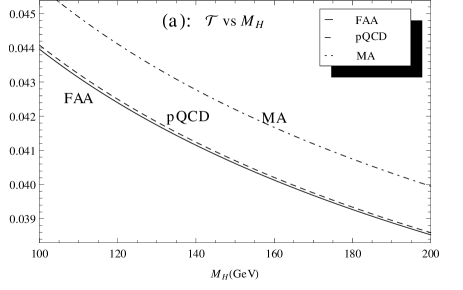
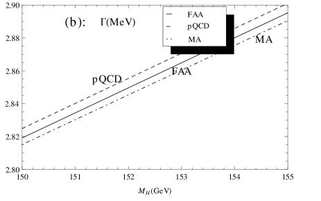
Figure 5: (a) The (dimensionless) quantity ${\cal T}(s)$, as defined in equation (68), as a function of the Higgs mass $M_{H}=\sqrt{s}$: for our approach (FAA) of equation (35), for the pQCD approach of equation (58) (in both cases ${\overline{\Lambda}}=0.213$ GeV at $n_{f}=5$); and for the minimal analytic (MA) model with FAA approach (${\overline{\Lambda}}_{\rm MA}=0.260$ GeV at $n_{f}=5$); (b) the same but now for the decay width $\Gamma(H\to b{\bar{b}})$.

We also include the curve for the Minimal Analytic (MA) model, evaluated by our method and using ${\overline{\Lambda}}(n_{f}=5)=0.260$ GeV. Our curve (FAA) can be interpreted as the result of application of our method in perturbative QCD, or in any such analytic QCD in which the values of the discontinuity function $\rho_{1}(\sigma)\equiv{\mathcal{A}}_{1}(-\sigma-i\epsilon)$ do not differ from the values of the pQCD discontinuity function $\rho_{1}^{\rm(pt)}(\sigma)\equiv a_{\rm pt}(-\sigma-i\epsilon)$ at $\sqrt{\sigma}\geq M_{H}$.

We see that the FAA and pQCD curves are close to each other. The MA curve for $\Gamma(H\to b{\bar{b}})$ comes close to the FAA and pQCD curves because the effects of different values of scales ${\overline{\Lambda}}$ ($0.260$ GeV instead of $0.213$ GeV) and different values of ${\hat{m}}_{b}^{2}$ [equations (73) instead of equation (64)] tend to cancel each other. The evaluation for the curves was performed by using the renormalization scales such that $|\mu^{2}|=s$ ($=M_{H}^{2}$). If we vary the value of the renormalization scale $|\mu^{2}|$ from $s/2$ to $2s$ around $s$, the values remain very stable; for example, when $M_{H}=150$ GeV, the values of ${\cal T}$ are $(4.062\pm 0.003)\cdot 10^{-2}$ in the FAA method case, and $(4.070\pm 0.001)\cdot 10^{-2}$ in the pQCD method case.

The decay width, by FAA method, is $\Gamma(H\to b{\bar{b}})=2.03,2.82,3.57$ MeV, when $M_{H}=100,150,200$ GeV, respectively.

It turns out that application of the expansion (54) in our FAA approach, instead of the expansion (35), gives the same result. Furthermore, the spacelike couplings ${\mathcal{A}}_{\nu}(Q^{2})$ obtained via equations (50) and (10), and the timelike couplings ${\mathfrak{A}}_{\nu}(Q^{2})$ obtained via equations (40) and (44) and (53), when evaluated in such analytic QCD models which have $\rho_{1}(\sigma)={\rm Im}a_{\rm pt}(-\sigma-i\epsilon)$, i.e., in MA-type models, give results numerically indistinguishable from the expressions [see also equation (2)]

$${\mathcal{A}}_{\nu}^{\rm(APT)}(Q^{2}) \equiv \frac{1}{\pi}\int_{0}^{\infty}\frac{d\sigma\ {\rm Im}a_{\rm pt}^{\nu}(-\sigma-i\epsilon)}{\sigma+Q^{2}}\ ,$$ (76)

$${\mathfrak{A}}_{\nu}^{\rm(APT)}(\sigma) \equiv \frac{1}{\pi}\int_{\sigma}^{\infty}\frac{d\sigma^{\prime}}{\sigma^{\prime}}{\rm Im}a_{\rm pt}^{\nu}(-\sigma^{\prime}-i\epsilon)\ ,$$ (77)

for any positive $\nu$ (in general noninteger); and $Q^{2}$ in the complex plane outside the negative semiaxis; and $\sigma>0$. This is another check of consistency of our method, because it shows that the APT construction, MSS ; Sh , of higher power analogs in MA of Shirkov and Solovtsov, when generalized from integer to noninteger powers ($n\mapsto\nu$) as in equations (76)-(77), gives the same result as our method.

Nonetheless, in conclusion, we stress that our method of construction of spacelike couplings ${\widetilde{\mathcal{A}}}_{\nu}$ and ${\mathcal{A}}_{\nu}$ [equations (10) and (50)], and of the corresponding timelike couplings ${\widetilde{\mathfrak{A}}}_{\nu}$ and ${\mathfrak{A}}_{\nu}$ [equations (40), (44), (53)] can be applied also to any other analytic QCD models, e.g., models where $\rho_{1}(\sigma)\not={\rm Im}a_{\rm pt}(-\sigma-i\epsilon)$. The latter inequality can be expected in general at low positive $\sigma$ values, cf. CCEM . In such models, the APT-type construction, equations (76)-(77), or modifications thereof, cannot be applied.

We recall that the timelike couplings ${\widetilde{\mathfrak{A}}}_{\nu}(\sigma)$ and ${{\mathfrak{A}}}_{\nu}(\sigma)$ of our (FAA) method depend only on $\rho_{1}(\sigma^{\prime})$ at $\sigma^{\prime}=\sigma e^{w}\geq\sigma$ – see equations (40), (44), (53). In the presented application of our method to $\Gamma(H\to b{\bar{b}})$, however, $\sigma=s=M_{H}^{2}>100^{2}\ {\rm GeV}^{2}$, i.e., only those $\rho_{1}(\sigma^{\prime})$ contribute for which $\sigma^{\prime}$ is very high ($>M_{H}^{2}$). At such high $\sigma^{\prime}$ we can expect that $\rho_{1}(\sigma^{\prime})={\rm Im}a_{\rm pt}(-\sigma^{\prime}-i\epsilon)$. Therefore, in such cases the formulas (77) for ${{\mathfrak{A}}}_{\nu}$’s can be applied [but not the formulas (76) for ${\mathcal{A}}_{\nu}$’s] and they give the same result for ${\mathfrak{A}}_{\nu}(\sigma)$ as our approach. Really, the FAA curve and the MA curve¡ in figs. 5 are numerically reproduced by application of equations (77), using the corresponding values ${\overline{\Lambda}}=0.213$ GeV and $0.260$ GeV, respectively.

It would also be interesting to apply our method to evaluation of low-energy timelike observables, where $\rho_{1}(\sigma)$ may differ significantly from the perturbative value. The method can also be applied to evaluation of spacelike quantities.

V Conclusions

We presented a method of calculating spacelike and timelike QCD observables whose perturbation expansion in perturbative QCD (pQCD) has noninteger powers of the perturbative coupling $a_{\rm pt}$ $(\equiv\alpha_{s}/\pi)$.

The method can be applied in any analytic QCD model, i.e., (a) in any model with a given analytic spacelike coupling ${\mathcal{A}}_{1}(Q^{2})$ (where ${\mathcal{A}}_{1}(Q^{2})$ is the analytic analog of spacelike $a_{\rm pt}(Q^{2})$); (b) or with a given discontinuity function $\rho_{1}(\sigma)\equiv{\rm Im}{\mathcal{A}}_{1}(-\sigma-i\epsilon)$ (where $\sigma\geq 0$). Specifically, first we constructed the analytic analogs ${\widetilde{\mathcal{A}}}_{\nu+1}(Q^{2})$ of the ($\nu$-noninteger extension) of the logarithmic derivatives ${\widetilde{a}}_{{\rm pt},\nu+1}(Q^{2})\propto d^{\nu}a_{\rm pt}(Q^{2})/d(\ln Q^{2})^{\nu+1}$, where $\nu$ can be any real number larger than $-2$, cf. equations (10), (22). Furthermore, we constructed the corresponding timelike (Minkowskian) couplings ${\widetilde{\mathfrak{A}}}_{\nu+1}(\sigma)$ ($\sigma\geq 0$), cf. equations (43), (49). Subsequently, we obtained the analytic spacelike couplings ${\mathcal{A}}_{\nu}(Q^{2})$ as a linear combination of the aforementioned ${\widetilde{\mathcal{A}}}_{\nu+m}(Q^{2})$’s ($m=0,1,2,\ldots$), where the couplings ${\mathcal{A}}_{\nu}(Q^{2})$ are analytic analogs (in any given analytic QCD models) of the powers $a_{\rm pt}(Q^{2})^{\nu}$ ($\nu$ any real number above $-1$), cf. equation (50). Furthermore, the corresponding timelike (Minkowskian) power analogs ${\mathfrak{A}}_{\nu}(\sigma)$ were constructed, as the corresponding linear combination of ${\widetilde{\mathfrak{A}}}_{\nu+m}(Q^{2})$ ($m=0,1,2,\ldots$), cf. (53).

We further demonstrated that in the Minimal Analytic model (MA, also named APT) of Shirkov, Solovtsov, Solovtsova and Milton ShS ; MSS ; Sh , our method gives the same explicit results for ${\mathcal{A}}_{\nu+1}(Q^{2})$ and ${\widetilde{\mathfrak{A}}}_{\nu+1}(\sigma)$ at the one-loop level as the method of BMS1 ; BMS2 ; BMS3 of Bakulev, Mikhailov and Stefanis (BMS; whose method can be applied in these MA-type models only), cf. equations (17) and (47). When going beyond the one-loop level within MA, the explicit formulas for ${\mathcal{A}}_{\nu+1}(Q^{2})$ and ${\widetilde{\mathfrak{A}}}_{\nu+1}(\sigma)$ in BMS1 ; BMS2 ; BMS3 become complicated and the comparison with our results becomes harder. Numerically, though, we have strong indications that within MA both BMS and our method agree also beyond the one-loop level. We recall that our results are given in form of integral, i.e., they are less explicit than the results of BMS1 ; BMS2 ; BMS3 for MA. However, our results are applicable in any analytic QCD, and look simple in its (integral) form.

When the analytic QCD model is based on a beta function $\beta({\mathcal{A}}_{1})$ which is analytic at ${\mathcal{A}}_{1}=0$ (CKV ), i.e., in perturbative analytic QCD, we simply obtain ${\mathcal{A}}_{n}={\mathcal{A}}_{1}^{n}$ CKV and ${\mathcal{A}}_{\nu}={\mathcal{A}}_{1}^{\nu}$.

Furthermore, our method can be applied to evaluation of timelike observables ${\cal T}(s)$ within the nonanalytic pQCD, provided that $s>\Lambda^{2}_{\rm L}$, where $\Lambda^{2}_{\rm L}$ is the positive branching point of the unphysical (Landau) $Q^{2}$-cut $(0,\Lambda^{2}_{\rm L})$ of $a_{\rm pt}(Q^{2})$. This latter approach can be described as a RGE-resummed contour method, as opposed to the more usual fixed-scale contour method in pQCD. On the other hand, for spacelike observables, while our method can be applied in (any) analytic QCD, it cannot be applied in nonanalytic pQCD, and the results are different from the usual (nonanalytic) pQCD evaluation results.

Further, if we work in an analytic QCD model for which the discontinuity function $\rho_{1}(\sigma)$ is equal to its pQCD counterpart $\rho_{1}^{\rm(pt)}(\sigma)$ for large enough $\sigma>M_{0}^{2}$ (where $M_{0}\sim 1\ {\rm GeV}>\Lambda_{\rm L}$, $M_{0}$ being a typical scale of the onset of pQCD), then the method gives for timelike observables ${\cal T}(s)$ at $s>M_{0}^{2}$ the same result as the method gives in nonanalytic pQCD. For spacelike observables no analogous statement holds. This is so because the spacelike couplings [${\mathcal{A}}_{1}(Q^{2})$, ${\widetilde{\mathcal{A}}}_{\nu}(Q^{2})$, ${\mathcal{A}}_{\nu}(Q^{2})$] are represented by integrals involving the values of $\rho_{1}(\sigma)$ along the entire cut of ${\mathcal{A}}_{1}(Q^{2})$, while the timelike couplings [${\mathfrak{A}}_{1}(s)$, ${\widetilde{\mathfrak{A}}}_{\nu}(s)$, ${\mathfrak{A}}_{\nu}(s)$] involve only $\rho_{1}(\sigma)$ for the cut sector $\sigma\in(s,+\infty)$.

We applied the method to evaluation of the Higgs decay width into $b{\bar{b}}$ pair $\Gamma(H\to b{\bar{b}})$, as a function of the Higgs mass $M_{H}$. The results of this evaluation turn out to be the same in pQCD and in any analytic QCD with $\rho_{1}(\sigma)=\rho_{1}^{\rm(pt)}(\sigma)$ at $\sigma\geq M_{H}^{2}$, because this is a high-energy timelike observable: $\Gamma(H\to b{\bar{b}})\propto{\cal T}(s)$ with $s=M_{H}^{2}\gg\Lambda_{\rm L}^{2}$.

It would be also interesting to apply our method in analytic QCD models to evaluation of low-energy timelike observables ${\cal T}(s)$ that involve noninteger powers, where $\rho_{1}(\sigma)$ at $\sigma\sim s$ may differ significantly from the perturbative value; and to evaluation of (low-energy) spacelike quantities in such models. For the latter, we plan to investigate the structure functions of the deep inelastic lepton-hadron scattering in analytic QCD models.

Appendix A Coefficients $k_{m}(\nu)$ and ${\widetilde{k}}_{m}(\nu)$

A.1 Coefficients $k_{m}(\nu)$: results

We need to find the coefficients $k_{m}(\nu)$, where $m=1,2,\ldots$, and $\nu$ is any real number. These coefficients are derived later in this appendix. First we write down their solution explicitly.

It turns out that they involve derivatives $Z_{m}(\nu+n)$ of the Riemannian $\Gamma$-functions

$$Z_{m}(\nu)\equiv\frac{1}{\Gamma(\nu+1)}\frac{d^{m}}{dx^{m}}{\left(\frac{\Gamma(\nu+1+x)}{\Gamma(1+x)}\right)}{\Big{|}}_{x=0}\ .$$ (78)

These functions can be expressed in the form of the Euler $\Psi$-functions and their derivatives

$$\Psi(\nu) \equiv \frac{d}{d\nu}\ln\Gamma(\nu)\ ,\quad\Psi^{(m)}(\nu)\equiv\frac{d^{m}}{d\nu^{m}}\Psi(\nu)\ .$$ (79)

$$S_{1}(\nu) \equiv \Psi(\nu+1)-\Psi(1)\ ,$$ (80)

$$S_{m}(\nu) \equiv \frac{(-1)^{m-1}}{(m-1)!}\,\left(\Psi^{(m-1)}(\nu+1)-\Psi^{(m-1)}(1)\right)\quad(m=2,3,\ldots)\ .$$ (81)

We note that $S_{m}(\nu)$ for integer $\nu=n$ (and $m=1,2,\ldots$) coincide with the usual harmonic numbers (of order $m$): $S_{m}(n)=\sum_{k=1}^{n}k^{-m}$. In terms of these functions, the functions $Z_{m}(\nu)$ of equation (78) are

$$Z_{0}(\nu) = 1\ ,\quad Z_{1}(\nu)=S_{1}(\nu)\ ,\quad Z_{2}(\nu)=S_{1}(\nu)^{2}-S_{2}(\nu)\ ,$$

$$Z_{3}(\nu) = S_{1}(\nu)^{3}-3S_{1}(\nu)S_{2}(\nu)+2S_{3}(\nu)\ ,$$

$$Z_{4}(\nu) = S_{1}(\nu)^{4}-6S_{1}(\nu)^{2}S_{2}(\nu)+3S_{2}(\nu)^{2}+8S_{1}(\nu)S_{3}(\nu)-6S_{4}(\nu)\ ,$$ (82)

In terms of the quantities $Z_{m}(\nu)$, as given by equation (78), the coefficients $k_{m}(\nu)$ are

$$k_{1}(\nu) = \nu\,c_{1}\,B_{1}(\nu),$$ (83)

$$k_{2}(\nu) = \nu(\nu+1)\,\bigg{(}c_{2}\,B_{2}(\nu)+\frac{c_{1}^{2}}{2}\,B_{1,1}(\nu)\biggr{)},$$ (84)

$$k_{3}(\nu) = \frac{\nu(\nu+1)(\nu+2)}{2}\bigg{(}c_{3}\,B_{3}(\nu)+c_{1}c_{2}\,B_{1,2}(\nu)+\frac{c_{1}^{3}}{3}\,B_{1,1,1}(\nu)\biggr{)},$$ (85)

$$k_{4}(\nu) = \frac{\nu(\nu+1)(\nu+2)(\nu+3)}{6}\bigg{(}c_{4}\,B_{4}(\nu)+c_{2}^{2}\,B_{2,2}(\nu)+\frac{c_{1}c_{3}}{2}\,B_{1,3}(\nu)+\frac{c_{1}^{2}c_{2}}{2}\,B_{1,1,2}(\nu)+\frac{c_{1}^{4}}{4}\,B_{1,1,1,1}(\nu)\biggr{)},$$ (86)

where

$$B_{1}(\nu) = Z_{1}(\nu)-1\ ,\quad B_{2}(\nu)=\frac{\nu-1}{2(\nu+1)}\ ,\quad B_{1,1}(\nu)=Z_{2}(\nu+1)-2\,Z_{1}(\nu)+1\ ,$$

$$B_{3}(\nu) = \frac{1}{6}-\frac{1}{\nu+1}+\frac{1}{\nu+2}\ ,\quad B_{1,2}(\nu)=\frac{\nu}{\nu+2}\,Z_{1}(\nu+1)+\frac{2}{\nu+1}+\frac{1}{\nu+2}-\frac{11}{6}\ ,$$

$$B_{1,1,1}(\nu) = Z_{3}(\nu+2)-3\,Z_{2}(\nu+1)+3\,Z_{1}(\nu)-1\ ,$$

$$B_{4}(\nu) = \frac{1}{12}-\frac{2}{(\nu+1)(\nu+2)(\nu+3)}\ ,\quad B_{2,2}(\nu)=\frac{5}{12}+\frac{1}{\nu+1}+\frac{1}{\nu+2}-\frac{5}{\nu+3}\ ,$$

$$B_{1,3}(\nu) = \left(1-\frac{6}{(\nu+2)(\nu+3)}\right)\,Z_{1}(\nu+1)+\frac{4}{\nu+1}-\frac{1}{\nu+2}-\frac{1}{\nu+3}-\frac{13}{6}\ ,$$

$$B_{1,1,2}(\nu) = \frac{3(\nu+1)}{\nu+3}Z_{2}(\nu+2)+\left(\frac{12}{\nu+2}+\frac{6}{\nu+3}-11\right)\,Z_{1}(\nu+1)-\frac{6}{\nu+1}-\frac{5}{\nu+2}-\frac{11}{\nu+3}+\frac{38}{3}\ ,$$

$$B_{1,1,1,1}(\nu) = Z_{4}(\nu+3)-4\,Z_{3}(\nu+2)+6\,Z_{2}(\nu+1)-4\,Z_{1}(\nu)+1\ .$$ (87)

A.2 Coefficients ${\widetilde{k}}_{m}(\nu)$: results

Inversion of the relations (28) gives us the expansion (29) and the ${\widetilde{k}}_{m}(\nu)$ coefficients in terms of the previously written coefficients $k_{\ell}(\nu+n)$ ($\ell=1,\ldots,m$, $n=0,1,\ldots,m-1$)

$${\widetilde{k}}_{1}(\nu) = k_{1}(\nu)\ ,\quad{\widetilde{k}}_{2}(\nu)=k_{1}(\nu)k_{1}(\nu+1)-k_{2}(\nu)\ ,$$

$${\widetilde{k}}_{3}(\nu) = -k_{1}(\nu)k_{1}(\nu+1)k_{1}(\nu+2)+k_{1}(\nu)k_{2}(\nu+1)+k_{1}(\nu+2)k_{2}(\nu)-k_{3}(\nu)\ ,$$

$${\widetilde{k}}_{4}(\nu) = k_{1}(\nu)k_{1}(\nu+1)k_{1}(\nu+2)k_{1}(\nu+3)-k_{1}(\nu)k_{1}(\nu+1)k_{2}(\nu+2)-k_{1}(\nu)k_{1}(\nu+3)k_{2}(\nu+1)$$ (88)

$$-k_{1}(\nu+2)k_{1}(\nu+3)k_{2}(\nu)+k_{2}(\nu)k_{2}(\nu+2)+k_{1}(\nu)k_{3}(\nu+1)+k_{1}(\nu+3)k_{3}(\nu)-k_{4}(\nu)\ .$$

It is possible to check that our formulas, equations (83)-(86) and (88), give

$$k_{n}(1)={\widetilde{k}}_{n}(1)=0\ ,$$ (89)

reflecting the fact that, by definition [equations (25) and (6)], ${\widetilde{\mathcal{A}}}_{1}\equiv{\mathcal{A}}_{1}$ and ${\widetilde{a}}_{{\rm pt},1}\equiv a_{\rm pt}$.

It is interesting that the coefficients ${\widetilde{k}}_{m}(\nu)$ can be cast in an equivalent alternative form which is somewhat similar to the expressions for the coefficients $k_{m}(\nu)$, equations (83)-(87), and where instead of the derivatives (78), another type of derivatives appears naturally:

$${\widetilde{Z}}_{m}(\nu)\equiv\Gamma(\nu+1)\frac{d^{m}}{dx^{m}}\left(\frac{\Gamma(1-x)}{\Gamma(\nu+1-x)}\right){\Big{|}}_{x=0}\ .$$ (90)

In terms of the harmonic numbers of order $k$, $S_{k}(n)=\sum_{s=1}^{n}s^{-k}$, functions $Z_{m}(n)$ and ${\widetilde{Z}}_{m}(n)$ can be expressed as

$$Z_{m}(n) \equiv \frac{1}{\Gamma(n+1)}\frac{d^{m}}{dx^{m}}{\left(\frac{\Gamma(n+1+x)}{\Gamma(1+x)}\right)}{\Big{|}}_{x=0}=\frac{d^{m}}{dx^{m}}\exp\left[\sum_{k=1}^{\infty}\frac{(-1)^{k+1}x^{k}}{k}S_{k}(n)\right]{\Big{|}}_{x=0}\ ,$$ (91)

$${\widetilde{Z}}_{m}(n) \equiv \Gamma(n+1)\frac{d^{m}}{dx^{m}}{\left(\frac{\Gamma(1-x)}{\Gamma(n+1-x)}\right)}{\Big{|}}_{x=0}=\frac{d^{m}}{dx^{m}}\exp\left[\sum_{k=1}^{\infty}\frac{x^{k}}{k}S_{k}(n)\right]{\Big{|}}_{x=0}\ .$$ (92)

This means that for ${\widetilde{Z}}_{m}$’s, formulas very similar to those of equations (82) for $Z_{m}$’s, are valid

$${\widetilde{Z}}_{0}(\nu) = 1(=Z_{0}(\nu))\ ,\quad{\widetilde{Z}}_{1}(\nu)=S_{1}(\nu)(=Z_{1}(\nu))\ ,\quad{\widetilde{Z}}_{2}(\nu)=S_{1}(\nu)^{2}+S_{2}(\nu)\ ,$$

$${\widetilde{Z}}_{3}(\nu) = S_{1}(\nu)^{3}+3S_{1}(\nu)S_{2}(\nu)+2S_{3}(\nu)\ ,$$

$${\widetilde{Z}}_{4}(\nu) = S_{1}(\nu)^{4}+6S_{1}(\nu)^{2}S_{2}(\nu)+3S_{2}(\nu)^{2}+8S_{1}(\nu)S_{3}(\nu)+6S_{4}(\nu)\ ,$$ (93)

The coefficients ${\widetilde{k}}_{m}(\nu)$ are then written in a form very similar to the formulas (83)-(86) for $k_{m}(\nu)$’s

$${\widetilde{k}}_{1}(\nu) = -\nu\,c_{1}\,{\widetilde{B}}_{1}(\nu),$$ (94)

$${\widetilde{k}}_{2}(\nu) = \nu(\nu+1)\,\bigg{(}-c_{2}\,{\widetilde{B}}_{2}(\nu)+\frac{c_{1}^{2}}{2}\,{\widetilde{B}}_{1,1}(\nu)\biggr{)},$$ (95)

$${\widetilde{k}}_{3}(\nu) = \frac{\nu(\nu+1)(\nu+2)}{2}\bigg{(}-c_{3}\,{\widetilde{B}}_{3}(\nu)+c_{1}c_{2}\,{\widetilde{B}}_{1,2}(\nu)-\frac{c_{1}^{3}}{3}\,{\widetilde{B}}_{1,1,1}(\nu)\biggr{)},$$ (96)

$${\widetilde{k}}_{4}(\nu) = \frac{\nu(\nu+1)(\nu+2)(\nu+3)}{6}\bigg{(}-c_{4}\,{\widetilde{B}}_{4}(\nu)\!+\!c_{2}^{2}\,{\widetilde{B}}_{2,2}(\nu)\!+\!\frac{c_{1}c_{3}}{2}\,{\widetilde{B}}_{1,3}(\nu)\!-\!\frac{c_{1}^{2}c_{2}}{2}\,{\widetilde{B}}_{1,1,2}(\nu)\!+\!\frac{c_{1}^{4}}{4}\,{\widetilde{B}}_{1,1,1,1}(\nu)\biggr{)},$$ (97)

where

$${\widetilde{B}}_{1}(\nu) = {\widetilde{Z}}_{1}(\nu)-1\ ,\quad{\widetilde{B}}_{2}(\nu)=\frac{\nu-1}{2(\nu+1)}\ ,\quad{\widetilde{B}}_{1,1}(\nu)={\widetilde{Z}}_{2}(\nu)-2\,{\widetilde{Z}}_{1}(\nu+1)+1\ ,$$

$${\widetilde{B}}_{3}(\nu) = \frac{1}{6}-\frac{1}{\nu+1}+\frac{1}{\nu+2}\ ,\quad{\widetilde{B}}_{1,2}(\nu)=\frac{\nu-1}{6(\nu+1)}\left(6{\widetilde{Z}}_{1}(\nu+1)-1+\frac{4}{\nu+2}\right)\ ,$$

$${\widetilde{B}}_{1,1,1}(\nu) = {\widetilde{Z}}_{3}(\nu)-3\,{\widetilde{Z}}_{2}(\nu+1)+3\,{\widetilde{Z}}_{1}(\nu+2)-1\ ,$$

$${\widetilde{B}}_{4}(\nu) = \frac{1}{12}-\frac{2}{(\nu+1)(\nu+2)(\nu+3)}\ ,\quad{\widetilde{B}}_{2,2}(\nu)=\frac{13}{12}-\frac{1}{\nu+1}-\frac{1}{\nu+2}-\frac{1}{\nu+3}\ ,$$

$${\widetilde{B}}_{1,3}(\nu) = \left(1-\frac{6}{(\nu+1)(\nu+2)}\right)\,{\widetilde{Z}}_{1}(\nu+3)+\frac{1}{6}+\frac{4}{\nu+1}-\frac{5}{\nu+2}-\frac{2}{\nu+3}\ ,$$

$${\widetilde{B}}_{1,1,2}(\nu) = \frac{3(\nu-1)}{\nu+1}{\widetilde{Z}}_{2}(\nu+2)-\left(1-\frac{6}{(\nu+1)(\nu+2)}\right)\,{\widetilde{Z}}_{1}(\nu+3)+\frac{8}{3}-\frac{2}{\nu+1}+\frac{1}{\nu+2}-\frac{8}{\nu+3}\ ,$$

$${\widetilde{B}}_{1,1,1,1}(\nu) = {\widetilde{Z}}_{4}(\nu)-4\,{\widetilde{Z}}_{3}(\nu+1)+6\,{\widetilde{Z}}_{2}(\nu+2)-4\,{\widetilde{Z}}_{1}(\nu+3)+1\ .$$ (98)

A.3 Reorganization of the power series; RS-dependence of new coefficients

The relation (29) between $a_{\rm pt}^{\nu}$ and ${\widetilde{a}}_{{\rm pt},\nu+m}$’s allows us to obtain immediately the relation between the coefficients ${\cal F}_{j}$ of the usual perturbative expansion (23) and the coefficients ${\widetilde{\cal F}}_{k}$ of the reorganized (“modified”) expansion (30)

$${\widetilde{\cal F}}_{1} = {\cal F}_{1}+{\widetilde{k}}_{1}(\nu_{0})\ ,$$ (99)

$${\widetilde{\cal F}}_{2} = {\cal F}_{2}+{\widetilde{k}}_{1}(\nu_{0}+1){\cal F}_{1}+{\widetilde{k}}_{2}(\nu_{0})\ ,$$ (100)

$${\widetilde{\cal F}}_{3} = {\cal F}_{3}+{\widetilde{k}}_{1}(\nu_{0}+2){\cal F}_{2}+{\widetilde{k}}_{2}(\nu_{0}+1){\cal F}_{1}+{\widetilde{k}}_{3}(\nu_{0})\ ,$$ (101)

$${\widetilde{\cal F}}_{4} = {\cal F}_{4}+{\widetilde{k}}_{1}(\nu_{0}+3){\cal F}_{3}+{\widetilde{k}}_{2}(\nu_{0}+2){\cal F}_{2}+{\widetilde{k}}_{3}(\nu_{0}+1){\cal F}_{1}+{\widetilde{k}}_{4}(\nu_{0})\ ,$$ (102)

All these are coefficients when the renormalization scale (RScl) $\mu^{2}$ is taken to be $\mu^{2}=Q^{2}$. If using another RScl $\mu^{2}\not=Q^{2}$ to calculate the observable ${\cal F}(Q^{2})$, we can obtain the RScl dependence of the coefficients ${\widetilde{\cal F}}_{j}(\mu^{2}/Q^{2})$ by using the relations $d{\widetilde{\mathcal{A}}}_{\nu}(\mu^{2})/d\ln\mu^{2}=-\beta_{0}\nu{\widetilde{\mathcal{A}}}_{\nu+1}(\mu^{2})$ [or equivalently: $d{\widetilde{a}}_{{\rm pt},\nu}(\mu^{2})/d\ln\mu^{2}=-\beta_{0}\nu{\widetilde{a}}_{{\rm pt},\nu+1}(\mu^{2})$], cf. equation 11), and the RScl independence of the (spacelike observable) ${\cal F}(Q^{2})$. The resulting expressions are

$${\widetilde{\cal F}}_{n}(\mu^{2}/Q^{2})={\widetilde{\cal F}}_{n}+\sum_{k=1}^{n}\frac{\Gamma(\nu_{0}+n)}{\Gamma(\nu_{0}+n-k)}\frac{1}{k!}\beta_{0}^{k}\ln^{k}\left(\frac{\mu^{2}}{Q^{2}}\right){\widetilde{\cal F}}_{n-k}\ ,$$ (103)

where we denote throughout ${\widetilde{\cal F}}_{k}\equiv{\widetilde{\cal F}}_{k}(1)$.

Since the coefficients ${\widetilde{k}}_{1}(\nu_{0}+n)$ are RScl independent, the relations (99)-(102) are valid at any RScl $\mu^{2}$, i.e., we can replace there ${\widetilde{\cal F}}_{j}\mapsto{\widetilde{\cal F}}_{j}(\mu^{2}/Q^{2})$ and ${\cal F}_{j}\mapsto{\cal F}_{j}(\mu^{2}/Q^{2})$.

A.4 Derivation of expressions for $k_{m}(\nu)$

In this Subsection, we will omit the subscript pt ($a_{\rm pt}\mapsto a$). Let’s consider the relation

$${\widetilde{a}}_{n+1}(Q^{2})=\left(\frac{(-1)}{n\beta_{0}}\,\frac{d}{d\left(\ln Q^{2}\right)}\right)\,{\widetilde{a}}_{n}(Q^{2}),$$ (104)

which is a consequence of the definition (25). In addition, we will use the following property:

$$\left(\frac{(-1)}{\beta_{0}}\,\frac{d}{d\left(\ln Q^{2}\right)}\right)\,a^{m}~{}=~{}m\;a^{m+1}\,\left(1+c_{1}a+c_{2}a^{2}+c_{3}a^{3}+c_{4}a^{4}+\dots\right)\ ,$$ (105)

which follows from the RGE, equation (26). We then obtain

$$\left(\frac{(-1)}{n\beta_{0}}\,\frac{d}{d\left(\ln Q^{2}\right)}\right)\,{\widetilde{a}}_{n}(Q^{2}) = a^{n+1}\,\left(1+{\cal K}_{1}(n)a^{1}+{\cal K}_{2}(n)a^{2}+{\cal K}_{3}(n)a^{3}+{\cal K}_{4}(n)a^{4}+\dots\right)$$ (106)

$$\cdot \left(1+c_{1}a+c_{2}a^{2}+c_{3}a^{3}+c_{4}a^{4}+\dots\right)\,,$$

where

$${\cal K}_{j}(n)~{}=~{}\frac{n+j}{n}\,k_{j}(n)$$ (107)

Equation (105) can be rewritten as

$${\widetilde{a}}_{n+1}(Q^{2}) = a^{n+1}\,\biggl{(}1+\left[{\cal K}_{1}(n)+c_{1}\right]a^{1}+\left[{\cal K}_{2}(n)+c_{1}{\cal K}_{1}(n)+c_{2}\right]a^{2}$$ (108)

$$+ \left[{\cal K}_{3}(n)+c_{1}{\cal K}_{2}(n)+c_{2}{\cal K}_{1}(n)+c_{3}\right]a^{3}$$

$$+ \left[{\cal K}_{4}(n)+c_{1}{\cal K}_{3}(n)+c_{2}{\cal K}_{2}(n)+c_{3}{\cal K}_{1}(n)+c_{4}\right]a^{3}+\dots\biggr{)}\,.$$

Comparing equations (28) and (108) we obtain the following recursive relations:

$$k_{1}(n+1) = \frac{(n+1)}{n}k_{1}(n)+c_{1}\,,$$ (109)

$$k_{2}(n+1) = \frac{(n+2)}{n}k_{2}(n)+c_{1}\frac{(n+1)}{n}k_{1}(n)+c_{2}\,,$$ (110)

$$k_{3}(n+1) = \frac{(n+3)}{n}k_{3}(n)+c_{1}\frac{(n+2)}{n}k_{2}(n)+c_{2}\frac{(n+1)}{n}k_{1}(n)+c_{3},$$ (111)

$$k_{4}(n+1) = \frac{(n+4)}{n}k_{4}(n)+c_{1}\frac{(n+3)}{n}k_{3}(n)+c_{2}\frac{(n+2)}{n}k_{2}(n)+c_{3}\frac{(n+1)}{n}k_{1}(n)+c_{4}\,.$$ (112)

We note that

$$k_{j}(2)=c_{j}\ ,\quad k_{j}(1)~{}=~{}0\,.$$ (113)

In order to solve the recursion relations (109)-(112), we find first solution to the following general recursion relation:

$$k(n+1)~{}=~{}\frac{n+\alpha_{1}}{n+\alpha_{2}}\,k(n)+c(n)\ ,$$ (114)

where $c(n)$ is some function of $n$ and $\alpha_{1}$ and $\alpha_{2}$ are some parameters.

If $c(n)=0$, then the solution of equation (114) is very simple

$$k(n)~{}=~{}\widetilde{c}\,\frac{\Gamma(n+\alpha_{1})}{\Gamma(n+\alpha_{2})}\ ,$$ (115)

where $\widetilde{c}$ is an arbitrary constant and $\Gamma$ is the Riemannian $\Gamma$-function.

If $c(n)\neq 0$, it is convenient to introduce a new variable $\hat{k}(n)$ which is related with $k(n)$ as

$$k(n)~{}=~{}\frac{\Gamma(n+\alpha_{1})}{\Gamma(n+\alpha_{2})}\,\hat{k}(n)\ .$$ (116)

Using equation (116) in equation (114) we obtain

$$\hat{k}(n+1)~{}=~{}\hat{k}(n)+\frac{\Gamma(n+\alpha_{2}+1)}{\Gamma(n+\alpha_{1}+1)}\,c(n)\ ,$$ (117)

with the solution

$$\hat{k}(n)~{}=~{}\hat{k}(s)+\sum_{j=s}^{n-1}\,\frac{\Gamma(j+\alpha_{2}+1)}{\Gamma(j+\alpha_{1}+1)}\,c(j)\ ,$$ (118)

where $s$ is a chosen number. Below it will be convenient to use $s=2$, because $k_{j}(2)=c_{j}$.

So, for $r(n)$, we have

$$k(n) = \frac{\Gamma(n+\alpha_{1})}{\Gamma(n+\alpha_{2})}\left[\frac{\Gamma(s+\alpha_{2})}{\Gamma(s+\alpha_{1})}\,k(s)+\sum_{j=s+1}^{n}\,\frac{\Gamma(j+\alpha_{2})}{\Gamma(j+\alpha_{1})}c(j-1)\right],$$ (119)

$$= \frac{\Gamma(n+\alpha_{1})}{\Gamma(n+\alpha_{2})}\left[\frac{\Gamma(2+\alpha_{2})}{\Gamma(2+\alpha_{1})}\,k(2)+\sum_{j=3}^{n}\,\frac{\Gamma(j+\alpha_{2})}{\Gamma(j+\alpha_{1})}c(j-1)\right],$$

Having the solution (119) to the recursion relation (114), we can proceed to solving the recursion relations (109)-(112).

1.   Consider the recursion (109): it corresponds to the general case with

$$k=k_{1},\quad\alpha_{1}=1,~{}~{}\alpha_{2}=0,~{}~{}c(n)=c_{1},~{}~{}k_{1}(2)=c_{1}\ .$$ (120)

So, using the solution (119), and $k_{1}(2)=c_{1}$, we have

$$k_{1}(n)~{}=~{}nc_{1}\left(\frac{1}{2}+\sum^{n}_{j=3}\frac{1}{j}\right)~{}=~{}nc_{1}\left(S_{1}(n)-1\right)\,$$ (121)

where

$$S_{m}(n)~{}=~{}\sum^{n}_{j=1}\frac{1}{j^{m}}$$ (122)

are harmonic numbers (of $m$’th order), which can be related with the $(m-1)$’th derivative of $\Psi$-function:

$$S_{1}(n) = \Psi(n+1)-\Psi(1),$$

$$S_{m+1}(n) = \frac{(-1)^{m}}{m!}\,\left(\Psi^{(m)}(n+1)-\Psi^{(m)}(1)\right),\quad\Psi^{(m)}(x+1)~{}=~{}\frac{d^{m}}{dx^{m}}\Psi(x+1)\ .$$ (123)

The $\Psi$-function is in turn the logarithmic derivative of the corresponding $\Gamma$-function:

$$\Psi(x+1)~{}=~{}\frac{d}{dx}\ln\Gamma(x+1)$$ (124)

and $\gamma=-\Psi(1)$ is Euler constant.

So, equation (121) can be represented in the following form:

$$k_{1}(n)~{}=~{}nc_{1}\biggl{(}\Psi(n+1)-\Psi(1)-1\biggr{)}~{}=~{}nc_{1}\biggl{(}\Psi(n+1)-\Psi(2)\biggr{)}\,,$$ (125)

which is well-defined also for noninteger values $n\mapsto\nu$

$$k_{1}(\nu)~{}=~{}\nu c_{1}\biggl{(}\Psi(\nu+1)-\Psi(2)\biggr{)}\,,$$ (126)

2.   Consider the recursion (110): it corresponds to the general case with

$$\alpha_{1} = 2,~{}~{}\alpha_{2}=0,~{}~{}k_{2}(2)=c_{2},~{}~{}$$

$$c(n) = c_{1}\cdot\frac{n+1}{n}k_{1}(n)+c_{2}=c_{1}^{2}\cdot(n+1)[S_{1}(n)-1]+c_{2}\,.$$ (127)

So, using the solution (119), we have

$$k_{2}(n)~{}=~{}n(n+1)\left(\frac{1}{6}c_{2}+\sum^{n}_{j=3}\frac{1}{j(j+1)}\biggl{\{}c_{2}+c_{1}^{2}\,j[S_{1}(j-1)-1]\biggl{\}}\right)$$ (128)

The coefficient in front of $c_{2}$ has the form

$$\frac{1}{6}+\sum^{n}_{j=3}\left(\frac{1}{j}-\frac{1}{j+1}\right)~{}=~{}\frac{1}{6}+\left(\sum^{n}_{j=3}-\sum^{n+1}_{j=4}\right)\frac{1}{j}~{}=~{}\frac{1}{6}+\left(\frac{1}{3}-\frac{1}{n+1}\right)~{}=~{}\frac{n-1}{2(n+1)}\ .$$ (129)

The coefficient in front of $c_{1}^{2}$ has the form

$$\sum^{n}_{j=3}\frac{1}{j+1}\,\biggl{(}S_{1}(j-1)-1\biggr{)}~{}=~{}\sum^{n}_{j=3}\left(\frac{S_{1}(j)}{j+1}-\frac{1}{j}\right)$$ (130)

Here, the second term on the right-hand side is

$$\sum^{n}_{j=3}\frac{1}{j}~{}=~{}S_{1}(n)-S_{1}(2)~{}=~{}S_{1}(n)-\frac{3}{2}\ ,$$ (131)

while the first term is

$$\sum^{n}_{j=3}\frac{S_{1}(j)}{j+1}~{}=~{}\sum^{n+1}_{j=4}\frac{S_{1}(j-1)}{j}~{}=~{}\frac{1}{2}\biggl{(}S_{1}^{2}(n+1)-S_{2}(n+1)\biggr{)}-1~{}\equiv\frac{1}{2}Z_{2}(n+1)-1,$$ (132)

where

$$Z_{m}(n)~{}=~{}\frac{1}{\Gamma(n+1)}\frac{d^{m}}{(dx^{m}}{\left(\frac{\Gamma(n+1+x)}{\Gamma(1+x)}\right)}{\Big{|}}_{x=0}=\frac{d^{m}}{dx^{m}}\exp\left[\sum_{k=1}^{\infty}\frac{(-1)^{k+1}x^{k}}{k}S_{k}(n)\right]{\Big{|}}_{x=0}\,.$$ (133)

For several first values, $Z_{m}(n)$ are

$$Z_{0}(n) = 1,~{}~{}~{}Z_{1}(n)~{}=~{}S_{1}(n),~{}~{}~{}Z_{2}(n)~{}=~{}S_{1}(n)^{2}-S_{2}(n)\,,$$

$$Z_{3}(n) = S_{1}(n)^{3}-3S_{1}(n)S_{2}(n)+2S_{3}(n)\,,$$

$$Z_{4}(n) = S_{1}(n)^{4}-6S_{1}(n)^{2}S_{2}(n)+8S_{1}(n)S_{3}(n)+3S_{2}(n)^{2}-6S_{4}(n)\,.$$ (134)

In the case noninteger values $n\mapsto\nu$, the ($m$’th) order harmonic numbers (122) are

$$S_{1}(\nu)~{}=~{}\Psi(\nu+1)-\Psi(1),~{}~{}S_{m}(\nu)~{}=~{}\frac{(-1)^{m-1}}{(m-1)!}\,\left(\Psi^{(m-1)}(\nu+1)-\Psi^{(m-1)}(1)\right)\,,$$ (135)

where

$$\Psi(\nu)~{}=~{}\frac{d}{(d\nu)}\ln\left(\Gamma(\nu)\right),~{}~{}~{}\Psi^{(m-1)}(\nu)~{}=~{}\frac{d^{m}}{d\nu^{m}}\Psi(\nu)$$ (136)

So, the result for $k_{2}(n)$ has the form

$$k_{2}(n)~{}=~{}\frac{n(n-1)}{2}\,c_{2}+\frac{n(n+1)}{2}\,c_{1}^{2}\cdot\left(Z_{2}(n+1)-2Z_{1}(n)+1\right)\ ,$$ (137)

which is well-defined also for noninteger values $n\mapsto\nu$

$$k_{2}(\nu)~{}=~{}\frac{\nu(\nu-1)}{2}\,c_{2}+\frac{\nu(\nu+1)}{2}\,c_{1}^{2}\cdot\left(Z_{2}(\nu+1)-2Z_{1}(\nu)+1\right)\ .$$ (138)

3.   The results for $k_{3}(n)$ and $k_{4}(n)$ can be obtained similarly. After the replacement $n\mapsto\nu$ they have the forms as given in equations (85)-(86) and (87).

Appendix B Large-$n$ behavior of coefficients

Here we calculate the asymptotical results for the coefficients ${\widetilde{\cal F}}_{n}$ at $n\to\infty$ of the expansion (30), assuming the standard Lipatov-type behavior Lipatov:1976ny ${\cal F}_{n}\sim n!$ for the coefficients ${\cal F}_{n}$ of the original expansion (23).

It is convenient to use the following form for the coefficients ${\cal F}_{n}$ at $n\to\infty$:

$${\cal F}_{n}=\frac{\Gamma(n+\nu_{0})}{\Gamma(\nu_{0})}b^{n}\,,$$ (139)

where $b\sim 1$ and $\Gamma$ is the Euler Gamma function.

From equations (99)-(102) we conclude that

$${\widetilde{\cal F}}_{n}=\sum_{m=0}^{n}{\widetilde{k}}_{n-m}(\nu_{0}+m){\cal F}_{m},~{}~{}{\widetilde{k}}_{0}=1,~{}~{}{\cal F}_{0}=1\,.$$ (140)

Firstly consider the first several terms on the right-hand side.

Let $m=n-1$. Due to equations (94) and (98), the right-hand side of (140) has the following form:

$${\widetilde{k}}_{1}(\nu_{0}+n-1){\cal F}_{n-1}=-c_{1}\nu\Bigl{[}{\widetilde{Z}}_{1}(\nu)-1\Bigr{]}\,\frac{\Gamma(\nu)}{\Gamma(\nu_{0})}b^{n-1}{\bigg{|}}_{\nu=\nu_{0}+n-1}=-c_{1}b^{n-1}\frac{\Gamma(n+\nu_{0})}{\Gamma(\nu_{0})}\Bigl{[}{\widetilde{Z}}_{1}(\nu_{0}+n-1)-1\Bigr{]}\,.$$

It can be rewritten also as

$${\widetilde{k}}_{1}(\nu_{0}+n-1)\frac{{\cal F}_{n-1}}{{\cal F}_{n}}=-\frac{c_{1}}{b}\Bigl{[}{\widetilde{Z}}_{1}(\nu_{0}+n-1)-1\Bigr{]}=-\frac{c_{1}}{b}\left(\frac{d}{dx}-1\right)\,\left(\frac{\Gamma(1-x)\Gamma(\nu_{0}+n)}{\Gamma(\nu_{0}+n-x)}\right){\Big{|}}_{x=0}\ ,$$

where we use equation (90) on the right-hand side.

At $m=n-2$ we have from (95) and (98)

$${\widetilde{k}}_{2}(\nu_{0}+n-2)\frac{{\cal F}_{n-2}}{{\cal F}_{n}}=\frac{1}{b^{2}}\bigg{(}-c_{2}\,{\widetilde{B}}_{2}(\nu_{0}+n-2)+\frac{c_{1}^{2}}{2}\,{\widetilde{B}}_{1,1}(\nu_{0}+n-2)\biggr{)}\,,$$

where at $n\to\infty$ (see equation (98))

$${\widetilde{B}}_{2}(\nu_{0}+n-2)\approx\frac{1}{2}\ ,\quad{\widetilde{B}}_{1,1}(\nu_{0}+n-2)\approx{\widetilde{Z}}_{2}(\nu_{0}+n-1)-2\,{\widetilde{Z}}_{1}(\nu_{0}+n-1)+1\ .$$

We use the simbol $\approx$ to show the asymptotics at $n\to\infty$. In particular, in the ${\widetilde{B}}_{1,1}$-case, the symbol $\approx$ involves the replacement of the argument $\nu_{0}+n-2$ in ${\widetilde{Z}}_{2}$ by $\nu_{0}+n-1$. Similar replacements will be used below.

So, we have

$${\widetilde{k}}_{2}(\nu_{0}+n-2)\frac{{\cal F}_{n-2}}{{\cal F}_{n}}\approx\frac{1}{2b^{2}}\left[c_{1}^{2}\left(\frac{d}{dx}-1\right)^{2}-c_{2}\right]\left(\frac{\Gamma(1-x)\Gamma(\nu_{0}+n)}{\Gamma(\nu_{0}+n-x)}\right){\Big{|}}_{x=0}\ .$$

When $m=n-3$, using (96) and (98) we have

$${\widetilde{k}}_{3}(\nu_{0}+n-3)\frac{{\cal F}_{n-3}}{{\cal F}_{n}}=\frac{1}{2b^{3}}\bigg{(}-c_{3}\,{\widetilde{B}}_{3}(\nu_{0}+n-3)+c_{1}c_{2}\,{\widetilde{B}}_{1,2}(\nu_{0}+n-3)-\frac{c_{1}^{3}}{3}\,{\widetilde{B}}_{1,1,1}(\nu_{0}+n-3)\biggr{)}\ ,$$

where at $n\to\infty$ (see equation (98))

$${\widetilde{B}}_{3}(\nu_{0}+n-3) \approx \frac{1}{6}\ ,\quad{\widetilde{B}}_{1,2}(\nu_{0}+n-3)\approx\left({\widetilde{Z}}_{1}(\nu_{0}+n-1)-\frac{1}{6}\right)\ ,$$

$${\widetilde{B}}_{1,1,1}(\nu_{0}+n-3) \approx {\widetilde{Z}}_{3}(\nu_{0}+n-1)-3\,{\widetilde{Z}}_{2}(\nu_{0}+n-1)+3\,{\widetilde{Z}}_{1}(\nu_{0}+n-1)-1\ .$$

Hence we have

$${\widetilde{k}}_{3}(\nu_{0}+n-3)\frac{{\cal F}_{n-3}}{{\cal F}_{n}}\approx\frac{1}{6b^{3}}\bigg{(}-\frac{c_{3}}{2}+3c_{1}c_{2}\,\left(\frac{d}{dx}-\frac{1}{6}\right)-c_{1}^{3}\,\left(\frac{d}{dx}-1\right)^{3}\biggr{)}\left(\frac{\Gamma(1-x)\Gamma(\nu_{0}+n)}{\Gamma(\nu_{0}+n-x)}\right){\Big{|}}_{x=0}\ .$$

Finally, when $m=n-4$, equations (96) and (98) lead to

$${\widetilde{k}}_{4}(\nu_{0}+n-4)\frac{{\cal F}_{n-4}}{{\cal F}_{n}} = \frac{1}{6b^{4}}\bigg{(}-c_{4}\,{\widetilde{B}}_{4}(\nu_{0}+n-4)+c_{2}^{2}\,{\widetilde{B}}_{2,2}(\nu_{0}+n-4)+\frac{c_{1}c_{3}}{2}\,{\widetilde{B}}_{1,3}(\nu_{0}+n-4)$$ (141)

$$-\frac{c_{1}^{2}c_{2}}{2}\,{\widetilde{B}}_{1,1,2}(\nu_{0}+n-4)+\frac{c_{1}^{4}}{4}\,{\widetilde{B}}_{1,1,1,1}(\nu_{0}+n-4)\biggr{)},$$

where at $n\to\infty$ (see equation (98))

$${\widetilde{B}}_{4}(\nu_{0}+n-4) \approx \frac{1}{12}\ ,\quad{\widetilde{B}}_{2,2}(\nu_{0}+n-4)\approx\frac{13}{12}\ ,\quad{\widetilde{B}}_{1,3}(\nu_{0}+n-4)\approx{\widetilde{Z}}_{1}(\nu_{0}+n-1)+\frac{1}{6}\ ,$$

$${\widetilde{B}}_{1,1,2}(\nu_{0}+n-4) \approx 3{\widetilde{Z}}_{2}(\nu_{0}+n-1)-{\widetilde{Z}}_{1}(\nu_{0}+n-1)+\frac{8}{3}\ ,$$

$${\widetilde{B}}_{1,1,1,1}(\nu_{0}+n-4) \approx {\widetilde{Z}}_{4}(\nu_{0}+n-1)-4\,{\widetilde{Z}}_{3}(\nu_{0}+n-1)+6\,{\widetilde{Z}}_{2}(\nu_{0}+n-1)-4\,{\widetilde{Z}}_{1}(\nu_{0}+n-1)+1\ .$$

So, we have

$${\widetilde{k}}_{4}(\nu_{0}+n-4)\frac{{\cal F}_{n-4}}{{\cal F}_{n}} \approx \frac{1}{24b^{4}}\bigg{(}\frac{13c_{2}^{2}-c_{4}}{3}+2c_{1}c_{3}\,\left(\frac{d}{dx}+\frac{1}{6}\right)-6c_{1}^{2}c_{2}\,\left[\left(\frac{d}{dx}-\frac{1}{6}\right)^{2}+\frac{31}{36}\right]$$ (142)

$$+c_{1}^{4}\,\left(\frac{d}{dx}-1\right)^{4}\biggr{)}\left(\frac{\Gamma(1-x)\Gamma(\nu_{0}+n)}{\Gamma(\nu_{0}+n-x)}\right){\Big{|}}_{x=0}\ .$$

B.1 Contributions of the powers of $c_{1}$

Taking only the terms $\sim c_{1}^{m}$ $(m=1,...,n)$, we have

$${\widetilde{\cal F}}_{n}^{(1)}={\cal F}_{n}\sum^{n}_{m=0}\frac{(-1)^{m}c_{1}^{m}}{m!\;b^{m}}\,\left(\frac{d}{dx}-1\right)^{m}\left(\frac{\Gamma(1-x)\Gamma(\nu_{0}+n)}{\Gamma(\nu_{0}+n-x)}\right){\Big{|}}_{x=0}\ .$$ (143)

At the beginning it is convenient to consider the sum on the right-hand side at $n\to\infty$. Moreover, the last term can be represented as

$$\frac{\Gamma(1-x)\Gamma(\nu_{0}+n)}{\Gamma(\nu_{0}+n-x)}=(\nu_{0}+n-1)\,\int_{0}^{1}dyy^{-x}(1-y)^{\nu_{0}+n-2}\,.$$

Application of the operator $(d/dx-\beta)$ to the term $y^{-x}$ has the simple form

$$\left(\frac{d}{dx}-\beta\right)^{m}\,y^{-x}=\left(\ln\frac{1}{y}-\beta\right)^{m}\,.$$

Then we have for the series on the right-hand side of (143) at $n\to\infty$

$$\sum^{n}_{m=0}\frac{(-1)^{m}c_{1}^{m}}{m!b^{m}}\,\left(\ln\frac{1}{y}-\beta\right)^{m}=\exp\left[-\frac{c_{1}}{b}\left(\ln\frac{1}{y}-\beta\right)\right]=y^{c_{1}/b}e^{c_{1}\beta/b}\,.$$

Thus, the contribution ${\widetilde{\cal F}}_{n}^{(1)}$ has the following form after integration on $y$:

$${\widetilde{\cal F}}_{n}^{(1)}={\cal F}_{n}R_{n}\left[e^{c_{1}/b}\frac{\Gamma(1+c_{1}/b)\Gamma(\nu_{0}+n)}{\Gamma(\nu_{0}+n+c_{1}/b)}\right]\,,$$

where the operation $R_{n}[F(c_{1})]$ takes the first $(n+1)$ terms of the expansion of $F$ in powers of $c_{1}$, and $R_{n}(x)\to x$ when $n\to\infty$.

Since $n$ is large, the difference between $R_{n}[F(c_{1})]$ and $F$ is very small ($\sim 1/(n+1)!$). So, we can omit the $R_{n}$ operation and take the contribution of the terms $\sim c_{1}^{m}$ $(m=1,...,n)$ in the form

$${\widetilde{\cal F}}_{n}^{(1)}\approx{\cal F}_{n}e^{c_{1}/b}\frac{\Gamma(1+c_{1}/b)\Gamma(\nu_{0}+n)}{\Gamma(\nu_{0}+n+c_{1}/b)}\,.$$ (144)

Note that the contribution ${\widetilde{\cal F}}_{n}^{(1)}$ is very important because the coefficient $c_{1}$ is universal and has nonzero value in ${\rm MS}$-like schemes. In the scheme where all $c_{j}=0$ $(j\geq 2)$, ${\widetilde{\cal F}}_{n}^{(1)}$ represents the full contribution to the reexpression of the expansion (23) to the one of equation (30): ${\widetilde{\cal F}}_{n}^{(1)}={\widetilde{\cal F}}_{n}$. As we can see in the next subsection, the contributions $\sim c_{j}$ $(j\geq 2)$ can be expressed also in the form $\sim{\widetilde{\cal F}}_{n}^{(1)}$.

Use of Stirling’s formula in (144) gives us

$${\widetilde{\cal F}}_{n}^{(1)}/{\cal F}_{n}\approx e^{c_{1}/b}\Gamma(1+c_{1}/b)\frac{1}{n^{c_{1}/b}}\ .$$ (145)

When the coefficients in the original series are nonalternating in sign, such as the one encountered in the Higgs decay width, equation (67), $b$ is positive and the above ratio even tends to zero when $n$ increases (we note that $c_{1}$ is positive for all $n_{f}\leq 6$).

Thus, the Lipatov-type asymptotics takes place for both ${\cal F}_{n}$ and ${\widetilde{\cal F}}_{n}$ coefficients in the $c_{j}=0$ ($j\geq 2$) scheme: only the subasymptotical terms are changed.

B.2 Contributions of $\sim c_{j}$ $(j\geq 2)$

The terms proportional to the first power of $c_{2}$ have the following form:

$${\widetilde{\cal F}}_{n}^{(2)}\approx{\cal F}_{n}\bigg{(}-\frac{c_{2}}{2b^{2}}+\frac{c_{1}c_{2}}{2b^{3}}\,\left(\frac{d}{dx}-\frac{1}{6}\right)-\frac{c_{1}^{2}c_{2}}{4b^{4}}\,\left[\left(\frac{d}{dx}-\frac{1}{6}\right)^{2}+\frac{31}{36}\right]+...\biggr{)}\left(\frac{\Gamma(1-x)\Gamma(\nu_{0}+n)}{\Gamma(\nu_{0}+n-x)}\right){\Big{|}}_{x=0}\ .$$

It is convenient at the first stage to exclude the term $\sim(31/36)c_{1}^{2}c_{2}$ from the consideration. It will be considered below together with the term $\sim c_{4}$.

Without the term $\sim(31/36)c_{1}^{2}c_{2}$, the contribution ${\widetilde{\cal F}}_{n}^{(2)}$ has the following form:

$${\widetilde{\cal F}}_{n}^{(2)}=-\frac{c_{2}}{2b^{2}}\,{\cal F}_{n}\sum^{n-2}_{m=0}\frac{(-1)^{m}c_{1}^{m}}{m!\;b^{m}}\,\left(\frac{d}{dx}-\frac{1}{6}\right)^{m}\left(\frac{\Gamma(1-x)\Gamma(\nu_{0}+n)}{\Gamma(\nu_{0}+n-x)}\right){\Big{|}}_{x=0}\ .$$ (146)

Repeating the calculations for ${\widetilde{\cal F}}_{n}^{(1)}$ done in the previous subsection we obtain for ${\widetilde{\cal F}}_{n}^{(2)}$

$${\widetilde{\cal F}}_{n}^{(2)}\approx-\frac{c_{2}}{2b^{2}}\,{\cal F}_{n}R_{n-2}\left[e^{c_{1}/(6b)}\frac{\Gamma(1+c_{1}/b)\Gamma(\nu_{0}+n)}{\Gamma(\nu_{0}+n+c_{1}/b)}\right]\,,$$

where, as in the previous subsection, the operation $R_{n-2}[F(c_{1})]$ takes the first $(n-1)$ terms of the expansion of $F$ on $c_{1}$.

Since $n$ is large, the difference between $R_{n-2}[F(c_{1})]$ and $F$ is very small. So, we can omit the $R_{n-2}$ operation and take the contribution of the terms $\sim c_{1}^{m}$ $(m=1,...,n-2)$ in the form

$${\widetilde{\cal F}}_{n}^{(2)}\approx-\frac{c_{2}}{2b^{2}}{\cal F}_{n}e^{c_{1}/(6b)}\frac{\Gamma(1+c_{1}/b)\Gamma(\nu_{0}+n)}{\Gamma(\nu_{0}+n+c_{1}/b)}\approx-\frac{c_{2}}{2b^{2}}{\widetilde{\cal F}}_{n}^{(1)}e^{-5c_{1}/(6b)}\,.$$ (147)

Taking the terms $\sim c_{3}$, we have

$${\widetilde{\cal F}}_{n}^{(3)} \approx {\cal F}_{n}\bigg{(}-\frac{c_{3}}{12b^{3}}+\frac{c_{1}c_{3}}{12b^{4}}\,\left(\frac{d}{dx}+\frac{1}{6}\right)+...\biggr{)}\left(\frac{\Gamma(1-x)\Gamma(\nu_{0}+n)}{\Gamma(\nu_{0}+n-x)}\right){\Big{|}}_{x=0}$$

$$= -\frac{c_{3}}{12b^{3}}\,{\cal F}_{n}\bigg{(}1+\frac{(-c_{1})^{1}}{1!\;b^{1}}\,\left(\frac{d}{dx}+\frac{1}{6}\right)+...\biggr{)}\left(\frac{\Gamma(1-x)\Gamma(\nu_{0}+n)}{\Gamma(\nu_{0}+n-x)}\right){\Big{|}}_{x=0}\ .$$

Repeating the above calcuations, we obtain

$${\widetilde{\cal F}}_{n}^{(3)}\approx-\frac{c_{3}}{12b^{3}}\,{\cal F}_{n}R_{n-3}\left[e^{-c_{1}/(6b)}\frac{\Gamma(1+c_{1}/b)\Gamma(\nu_{0}+n)}{\Gamma(\nu_{0}+n+c_{1}/b)}\right]\ ,$$

and, because $n$ is large,

$${\widetilde{\cal F}}_{n}^{(3)}\approx-\frac{c_{3}}{12b^{3}}{\widetilde{\cal F}}_{n}^{(1)}e^{-7c_{1}/(6b)}\,.$$ (148)

Now we consider the remaining terms $\sim 1/b^{4}$. At the leading order (in $c_{1}$), they contribute in two places: as the term $\sim(13c_{2}^{2}-c_{4})$ in equation (142) and as the term $\sim(31/36)c_{1}^{2}c_{2}$ in the first equation of this subsection. Taking them together we have, at the leading order in $c_{1}$

$${\widetilde{\cal F}}_{n}^{(4)}\approx-\frac{(2c_{4}-26c_{2}^{2}+31c_{1}^{2}c_{2})}{144b^{4}}\,{\cal F}_{n}\ .$$

Adding to this the terms of relative higher order in $c_{1}$, in analogy with above calculations for ${\widetilde{\cal F}}_{n}^{(j)}$ $(j=2,3)$, gives

$${\widetilde{\cal F}}_{n}^{(4)}\approx-\frac{(2c_{4}-26c_{2}^{2}+31c_{1}^{2}c_{2})}{144b^{4}}\,{\widetilde{\cal F}}_{n}^{(1)}e^{-(\hat{k}+1)c_{1}/b}\,.$$ (149)

To find the exact value of the factor $\hat{k}$ we should calculate the term ${\widetilde{k}}_{5}(\nu_{0}+n-5){\cal F}_{n-5}/{\cal F}_{n}$ in analogy with (142). It needs in turn the calculaton of the coefficients ${\widetilde{k}}_{5}$ and, thus, one step more in the analysis in appendix A. Hovewer, looking carefully at the above calculations, we note that the coefficients in the exponents, in front of $-c_{1}/b$, rise with the index $j$ of ${\widetilde{\cal F}}_{n}^{(j)}$ . For ${\widetilde{\cal F}}_{n}^{(3)}$ the corresponding coefficient is equal to $7/6$ and we suggest that $\hat{k}$ in (149) should be bigger.

So, we have for the coefficient ${\widetilde{\cal F}}_{n}$ the following approximation at large $n$ values:

$${\widetilde{\cal F}}_{n}\approx{\widetilde{\cal F}}_{n}^{(1)}\,\left(1-\frac{c_{2}}{2b^{2}}e^{-5c_{1}/(6b)}-\frac{c_{3}}{12b^{3}}e^{-7c_{1}/(6b)}-\frac{(2c_{4}-26c_{2}^{2}+31c_{1}^{2}c_{2})}{144b^{4}}\,e^{-(\hat{k}+1)c_{1}/b}-...\right)\,.$$ (150)

We see that the corrections from $\sim c_{j}$ $(j\geq 2)$ have the same sign and are decreasing in magnitude. Indeed, for $b=1$, and when $n_{f}=5$, we have

$$b=1,~{}~{}c_{1}=1.2609,~{}~{}c_{2}=1.4748,~{}~{}c_{3}=9.8357,~{}~{}c_{4}\approx 86.\ ,$$

and these corrections apparently have decreasing magnitudes

$${\widetilde{\cal F}}_{n}\approx{\widetilde{\cal F}}_{n}^{(1)}\,\left(1-0.258-0.188-1.3\times(0.283)^{(\hat{k}+1)}-...\right)\,,$$ (151)

where $\exp[-(\hat{k}+1)c_{1}]\approx(0.283)^{(\hat{k}+1)}<0.23$ if $\hat{k}\geq 1/6$.

Thus, the contributions of $\sim c_{j}$ $(j\geq 2)$ are rather small and can be expressed through the contribution of $\sim c_{1}$.

Appendix C Proof of equation (43)

We prove the formula of equation (43) by mathematical induction with respect to $n=0,1,\ldots$. For $n=0$, this is the formula of equation (40) which was proven in the text. Now suppose that the formula equation (43) is valid for a given $n$. We will show that then it must be valid also for $n+1$.

If the formula of equation (43) is valid for a given $n$, we can use it and the recursion relation (42) to obtain

$${\widetilde{\mathfrak{A}}}_{\delta+n+2}(\sigma) = \frac{(-1)\sin(\pi(\delta+n))}{\pi^{2}(\delta+n+1)(\delta+n)\beta_{0}^{\delta+n+1}}$$ (153)

$$\times\int_{\epsilon}^{\infty}\frac{dw}{w^{\delta+n}}\left[\frac{\partial\rho_{1}(\sigma e^{w})}{\partial w}-\frac{d\rho_{1}(\sigma)}{d\ln\sigma}-\frac{w}{1!}\frac{d^{2}\rho_{1}(\sigma)}{d(\ln\sigma)^{2}}-\ldots-\frac{w^{n-1}}{(n-1)!}\frac{d^{n}\rho_{1}(\sigma)}{d(\ln\sigma)^{n}}\right]$$

$$= \frac{\sin(\pi(\delta+n+1))}{\pi^{2}(\delta+n+1)\beta_{0}^{\delta+n+1}}{\bigg{\{}}\int_{\epsilon}^{\infty}\frac{dw\rho_{1}(\sigma e^{w})}{w^{\delta+n+1}}-\frac{1}{(\delta+n)\epsilon^{\delta+n}}\rho_{1}(\sigma e^{\epsilon})-\frac{1}{(\delta+n)(\delta+n-1)\epsilon^{\delta+n-1}}\frac{d\rho_{1}(\sigma)}{d\ln\sigma}$$

$$-\frac{1}{(\delta+n)(\delta+n-2)1!\;\epsilon^{\delta+n-2}}\frac{d^{2}\rho_{1}(\sigma)}{d(\ln\sigma)^{2}}-\cdots-\frac{1}{(\delta+n)(\delta+n-k)(k-1)!\;\epsilon^{\delta+n-k}}\frac{d^{k}\rho_{1}(\sigma)}{d(\ln\sigma)^{k}}-\cdots$$

$$-\frac{1}{(\delta+n)(\delta)(n-1)!\;\epsilon^{\delta}}\frac{d^{n}\rho_{1}(\sigma)}{d(\ln\sigma)^{n}}{\big{\}}}\ .$$

Here it is understood that $\epsilon\to+0$; and in the step from equation (153) to equation (153) we performed integration by parts in the first term.

Now we use in $\rho_{1}(\sigma e^{\epsilon})$ Taylor expansion in logarithm of the argument ($\ln\sigma+\epsilon$)

$$\rho_{1}(\sigma e^{\epsilon})=\rho_{1}(\sigma)+\sum_{k=1}^{n}\frac{\epsilon^{k}}{k!}\frac{d^{k}\rho_{1}(\sigma)}{(d\ln\sigma)^{k}}+{\cal O}(\epsilon^{n+1})\ ,$$ (154)

in the above expression (153), and obtain

$${\widetilde{\mathfrak{A}}}_{\delta+n+2}(\sigma) = \frac{\sin(\pi(\delta+n+1))}{\pi^{2}(\delta+n+1)\beta_{0}^{\delta+n+1}}{\bigg{\{}}\int_{\epsilon}^{\infty}\frac{dw\rho_{1}(\sigma e^{w})}{w^{\delta+n+1}}-\frac{\rho_{1}(\sigma)}{(\delta+n)\epsilon^{\delta+n}}$$ (155)

$$-\sum_{k=1}^{n}\frac{1}{\epsilon^{\delta+n-k}(\delta+n)}\left[\frac{1}{k!}+\frac{1}{(\delta+n-k)(k-1)!}\right]\frac{d^{k}\rho_{1}(\sigma)}{(d\ln\sigma)^{k}}+{\cal O}(\epsilon^{1-\delta}){\bigg{\}}}\ .$$

Using the identity

$$\left[\frac{1}{k!}+\frac{1}{(\delta+n-k)(k-1)!}\right]=\frac{1}{k!}\frac{(\delta+n)}{(\delta+n-k)}\ ,$$ (156)

we can rewrite the expression (155) as

$${\widetilde{\mathfrak{A}}}_{\delta+n+2}(\sigma) = \frac{\sin(\pi(\delta+n+1))}{\pi^{2}(\delta+n+1)\beta_{0}^{\delta+n+1}}\int_{\epsilon}^{\infty}\frac{dw}{w^{\delta+n+1}}{\bigg{\{}}\rho_{1}(\sigma e^{w})-\rho_{1}(\sigma)-\sum_{k=1}^{n}\frac{1}{k!}w^{k}\frac{d^{k}\rho_{1}(\sigma)}{(d\ln\sigma)^{k}}{\bigg{\}}}+{\cal O}(\epsilon^{1-\delta})\ .$$ (157)

Since $0<\delta<1$, we are now allowed to take the limit $\epsilon\to+0$ in the above integral ($\epsilon^{1-\delta}\to 0$) and we conclude that the identity (43) is valid also for $n+1$. This concludes the proof of identity (43) via mathematical induction.

Appendix D Coefficients of expansion of ${\overline{\rm MS}}$ squared mass

Integration of the RGE’s (26) and (62) gives for the ${\overline{\rm MS}}$ squared running mass the solution in the form of expansion (63), with the coefficients ${\cal M}_{j}$ there being (note that $\gamma_{0}=1$)

$${\cal M}_{1} = -\frac{2}{\beta_{0}}(c_{1}-\gamma_{1})\ ,$$ (158)

$${\cal M}_{2} = \frac{1}{2}{\cal M}_{1}^{2}-\frac{1}{\beta_{0}}\left((c_{2}-\gamma_{2})-c_{1}(c_{1}-\gamma_{1})\right)\ ,$$ (159)

$${\cal M}_{3} = -\frac{1}{3}{\cal M}_{1}^{3}+{\cal M}_{1}{\cal M}_{2}-\frac{2}{3\beta_{0}}\left((c_{3}-\gamma_{3})-c_{1}(c_{2}-\gamma_{2})+(c_{1}^{2}-c_{2})(c_{1}-\gamma_{1})\right)\ ,$$ (160)

$${\cal M}_{4} = \frac{1}{4}{\cal M}_{1}^{4}-{\cal M}_{1}^{2}{\cal M}_{2}+\frac{1}{2}{\cal M}_{2}^{2}+{\cal M}_{1}{\cal M}_{3}$$ (161)

$$-\frac{1}{2\beta_{0}}\left((c_{4}-\gamma_{4})-c_{1}(c_{3}-\gamma_{3})+(c_{1}^{2}-c_{2})(c_{2}-\gamma_{2})+(-c_{1}^{3}+2c_{1}c_{2}-c_{3})(c_{1}-\gamma_{1})\right)\ .$$

References

- (1) N.N. Bogoliubov and D.V. Shirkov, Introduction to the Theory of Quantum Fields, New York, Wiley, 1959; 1980.
- (2) R. Oehme, Int. J. Mod. Phys. A 10, 1995 (1995) [arXiv:hep-th/9412040].
- (3) D. V. Shirkov and I. L. Solovtsov, hep-ph/9604363; Phys. Rev. Lett. 79, 1209 (1997) [arXiv:hep-ph/9704333].
- (4) K. A. Milton, I. L. Solovtsov and O. P. Solovtsova, Phys. Lett. B 415, 104 (1997) [arXiv:hep-ph/9706409].
- (5) D. V. Shirkov, Theor. Math. Phys. 127, 409 (2001) [hep-ph/0012283]; Eur. Phys. J. C 22, 331 (2001) [hep-ph/0107282].
- (6) A. V. Nesterenko, Phys. Rev. D 62, 094028 (2000) [arXiv:hep-ph/9912351]; Phys. Rev. D 64, 116009 (2001) [arXiv:hep-ph/0102124]; Int. J. Mod. Phys. A 18, 5475 (2003) [arXiv:hep-ph/0308288].
- (7) A. I. Karanikas and N. G. Stefanis, Phys. Lett. B 504, 225 (2001) [Erratum-ibid. B 636, 330 (2006)] [arXiv:hep-ph/0101031].
- (8) G. M. Prosperi, M. Raciti and C. Simolo, Prog. Part. Nucl. Phys. 58, 387 (2007) [arXiv:hep-ph/0607209].
- (9) D. V. Shirkov and I. L. Solovtsov, Theor. Math. Phys. 150, 132 (2007) [arXiv:hep-ph/0611229].
- (10) G. Cvetič and C. Valenzuela, Braz. J. Phys. 38, 371 (2008) [arXiv:0804.0872 [hep-ph]].
- (11) A. P. Bakulev, Phys. Part. Nucl. 40, 715 (2009) (in Russian) [arXiv:0805.0829 [hep-ph]].
- (12) R. S. Pasechnik, D. V. Shirkov, O. V. Teryaev, Phys. Rev. D78, 071902 (2008) [arXiv:0808.0066 [hep-ph]]; R. S. Pasechnik, D. V. Shirkov, O. V. Teryaev, O. P. Solovtsova, V. L. Khandramai, Phys. Rev. D81, 016010 (2010) [arXiv:0911.3297 [hep-ph]]; R. S. Pasechnik, J. Soffer, O. V. Teryaev, Phys. Rev. D82, 076007 (2010) [arXiv:1009.3355 [hep-ph]].
- (13) V. I. Khandramai, R. S. Pasechnik, D. V. Shirkov, O. P. Solovtsova, O. V. Teryaev, Phys. Lett. B 706, 340 (2012) [arXiv:1106.6352 [hep-ph]].
- (14) S. Schael et al. [ALEPH Collaboration], Phys. Rept. 421, 191 (2005) [hep-ex/0506072]; M. Davier, A. Höcker and Z. Zhang, Rev. Mod. Phys. 78, 1043 (2006) [hep-ph/0507078].
- (15) M. Davier, S. Descotes-Genon, A. Höcker, B. Malaescu and Z. Zhang, Eur. Phys. J. C 56, 305 (2008) [arXiv:0803.0979 [hep-ph]].
- (16) K. A. Milton, I. L. Solovtsov, O. P. Solovtsova and V. I. Yasnov, Eur. Phys. J. C 14, 495 (2000) [arXiv:hep-ph/0003030].
- (17) K. A. Milton, I. L. Solovtsov and O. P. Solovtsova, Phys. Rev. D 64, 016005 (2001) [arXiv:hep-ph/0102254]. Mod. Phys. Lett. A 21, 1355 (2006) [hep-ph/0512209].
- (18) B. V. Geshkenbein, B. L. Ioffe and K. N. Zyablyuk, Phys. Rev. D 64, 093009 (2001) [arXiv:hep-ph/0104048].
- (19) G. Cvetič, R. Kögerler, C. Valenzuela, J. Phys. G G37, 075001 (2010) [arXiv:0912.2466 [hep-ph]]; Phys. Rev. D82, 114004 (2010) [arXiv:1006.4199 [hep-ph]].
- (20) G. Cvetič and C. Valenzuela, J. Phys. G 32, L27 (2006) [arXiv:hep-ph/0601050].
- (21) G. Cvetič and C. Valenzuela, Phys. Rev. D 74, 114030 (2006) [arXiv:hep-ph/0608256].
- (22) D. V. Shirkov, Nucl. Phys. Proc. Suppl. 162, 33 (2006) [arXiv:hep-ph/0611048].
- (23) D. V. Shirkov, Theor. Math. Phys. 119, 438 (1999) [Teor. Mat. Fiz. 119, 55 (1999)] [arXiv:hep-th/9810246]; Lett. Math. Phys. 48, 135 (1999).
- (24) A. P. Bakulev, S. V. Mikhailov and N. G. Stefanis, Phys. Rev. D 72, 074014 (2005) [Erratum-ibid. D 72, 119908 (2005)] [arXiv:hep-ph/0506311].
- (25) A. P. Bakulev, S. V. Mikhailov and N. G. Stefanis, Phys. Rev. D 75, 056005 (2007) [Erratum-ibid. D 77, 079901 (2008)] [arXiv:hep-ph/0607040].
- (26) A. P. Bakulev, S. V. Mikhailov and N. G. Stefanis, JHEP 1006, 085 (2010) [arXiv:1004.4125 [hep-ph]].
- (27) A. P. Bakulev, I. V. Potapova, Nucl. Phys. Proc. Suppl. 219-220, 193 (2011) [arXiv:1108.6300 [hep-ph]].
- (28) Mathematica 8.0.4, Wolfram Co.
- (29) A. Erdélyi, W. Magnus, F. Oberhettinger and F. G. Tricomi, Higher Transcendental Functions, Vol. I, McGraw-Hill Book Company, Inc., New York-Toronto-London. 1953; note that they use for the Lerch function notation: .
- (30) A. P. Prudnikov, Yu. A. Brychkov, and O. I. Marichev, Integrals and Series, Vol. 3: More Special Functions, New York, Gordon and Breach (1989); I. S. Gradshteyn and I. M. Ryzhik, Table of Integrals, series, and Products, 7th edition, edited by A. Jeffrey and D. Zwillinger, Academic Press, London, 2007
- (31) A. V. Kotikov, V. G. Krivokhizhin and B. G. Shaikhatdenov, arXiv:1008.0545 [hep-ph], Phys. Atom. Nucl. 75, 507 (2012)
- (32) D. I. Kazakov and D. V. Shirkov, Fortsch. Phys. 28, 465 (1980).
- (33) D. V. Shirkov, arXiv:1202.3220 [hep-ph].
- (34) L. N. Lipatov, Sov. Phys. JETP 45, 216 (1977) [Zh. Eksp. Teor. Fiz. 72, 411 (1977)].
- (35) G. Cvetič, M. Loewe, C. Martínez and C. Valenzuela, Phys. Rev. D 82, 093007 (2010) [arXiv:1005.4444 [hep-ph]].
- (36) A. Djouadi, Phys. Rept. 457, 1 (2008) [arXiv:hep-ph/0503172].
- (37) A. L. Kataev and V. T. Kim, PoS A CAT08, 004 (2008) [arXiv:0902.1442 [hep-ph]]; D. J. Broadhurst, A. L. Kataev and C. J. Maxwell, Nucl. Phys. B 592, 247 (2001) [arXiv:hep-ph/0007152].
- (38) K. G. Chetyrkin, B. A. Kniehl and A. Sirlin, Phys. Lett. B 402, 359 (1997) [arXiv:hep-ph/9703226].
- (39) R. Tarrach, Nucl. Phys. B 183, 384 (1981).
- (40) O. V. Tarasov, preprint JINR-P2-82-900, Dec 1982; S. A. Larin, Phys. Lett. B 303, 113 (1993) [arXiv:hep-ph/9302240].
- (41) K. G. Chetyrkin, Phys. Lett. B 404, 161 (1997) [arXiv:hep-ph/9703278]; J. A. M. Vermaseren, S. A. Larin and T. van Ritbergen, Phys. Lett. B 405, 327 (1997) [arXiv:hep-ph/9703284].
- (42) D. J. Gross and F. Wilczek, Phys. Rev. Lett. 30, 1343 (1973); H. D. Politzer, Phys. Rev. Lett. 30, 1346 (1973).
- (43) W. E. Caswell, Phys. Rev. Lett. 33, 244 (1974); D. R. T. Jones, Nucl. Phys. B 75, 531 (1974); E. Egorian and O. V. Tarasov, Teor. Mat. Fiz. 41, 26 (1979) [Theor. Math. Phys. 41, 863 (1979)].
- (44) O. V. Tarasov, A. A. Vladimirov and A. Y. Zharkov, Phys. Lett. B 93, 429 (1980).
- (45) T. van Ritbergen, J. A. M. Vermaseren and S. A. Larin, Phys. Lett. B 400, 379 (1997) [arXiv:hep-ph/9701390].
- (46) J. R. Ellis, I. Jack, D. R. T. Jones, M. Karliner and M. A. Samuel, Phys. Rev. D 57, 2665 (1998) [arXiv:hep-ph/9710302].
- (47) K. Nakamura et al. [Particle Data Group], J. Phys. G 37, 075021 (2010).
- (48) C. Contreras, G. Cvetič and P. Gaete, Phys. Rev. D 70, 034008 (2004) [arXiv:hep-ph/0311202]; Nucl. Phys. Proc. Suppl. 152, 140 (2006) [arXiv:hep-ph/0410220].¡
- (49) K. G. Chetyrkin, B. A. Kniehl and M. Steinhauser, Nucl. Phys. B 510, 61 (1998) [arXiv:hep-ph/9708255].
- (50) K. G. Chetyrkin, Phys. Lett. B 390, 309 (1997) [arXiv:hep-ph/9608318].
- (51) P. A. Baikov, K. G. Chetyrkin and J. H. Kühn, Phys. Rev. Lett. 96, 012003 (2006) [arXiv:hep-ph/0511063].
- (52) C. Contreras, G. Cvetič, O. Espinosa and H. E. Martínez, Phys. Rev. D 82, 074005 (2010) [arXiv:1006.5050].
- (53) A. I. Alekseev, Few Body Syst. 40, 57 (2006) [arXiv:hep-ph/0503242].
- (54) E. Gardi, G. Grunberg and M. Karliner, JHEP 9807, 007 (1998) [hep-ph/9806462].
- (55) B. A. Magradze, arXiv:hep-ph/9808247; Few Body Syst. 40, 71 (2006) [arXiv:hep-ph/0512374].
- (56) D. S. Kourashev, arXiv:hep-ph/9912410; D. S. Kurashev and B. A. Magradze, Theor. Math. Phys. 135, 531 (2003) [Teor. Mat. Fiz. 135, 95 (2003)].
- (57) A. V. Kotikov and V. N. Velizhanin, arXiv:hep-ph/0501274; A. V. Kotikov, Phys. Atom. Nucl. 57, 133 (1994) [Yad. Fiz. 57, 142 (1994)].