Holographic Duals of $D=3$ ${\mathcal{N}}=4$ Superconformal Field Theories

Abstract

We find the warped $AdS_{4}\ltimes K$ type-IIB supergravity solutions holographically dual to a large family of three dimensional ${\mathcal{N}}=4$ superconformal field theories labeled by a pair $(\rho,\hat{\rho})$ of partitions of $N$. These superconformal theories arise as renormalization group fixed points of three dimensional mirror symmetric quiver gauge theories, denoted by $T^{\rho}_{\hat{\rho}}(SU(N))$ and $T_{\rho}^{\hat{\rho}}(SU(N))$ respectively. We give a supergravity derivation of the conjectured field theory constraints that must be satisfied in order for these gauge theories to flow to a non-trivial supersymmetric fixed point in the infrared. The exotic global symmetries of these superconformal field theories are precisely realized in our explicit supergravity description.

LPTENS-11/21

^♮ Laboratoire de Physique Théorique de l’École Normale Supérieure,

24 rue Lhomond, 75231 Paris cedex, France

^♭ Instituut voor Theoretische Fysica, Katholieke Universiteit Leuven,

Celestijnenlaan 200D B-3001 Leuven, Belgium

^† Perimeter Institute for Theoretical Physics,

Waterloo, Ontario, N2L2Y5, Canada

1 Introduction

The gauge/gravity duality conjecturally imprints the dynamics of a $D$-dimensional conformal field theory (CFT) in the physics of string/M-theory with asymptotically $AdS_{D+1}\ltimes K$ warped boundary conditions. The information about the specific CFT is encoded in the geometry of the internal manifold $K$, the fluxes supporting the $AdS_{D+1}\ltimes K$ background, together with the possible presence of branes or singularities in the geometry. In the celebrated paper by Maldacena [1] the string/M-theory backgrounds for the maximally supersymmetric conformal field theories in $D=3,4$ and $6$ were identified. In particular, the M-theory background $AdS_{4}\times S^{7}$ was advanced as the holographic bulk description of the three-dimensional ${\mathcal{N}}=8$ superconformal field theory arising in the extreme infrared limit of maximally supersymmetric three-dimensional Yang-Mills with gauge group $SU(N)$.

In this paper we construct the warped $AdS_{4}\ltimes K$ backgrounds of type-IIB string theory dual to a rich family of three dimensional ${\mathcal{N}}=4$ superconformal field theories labeled by a pair $(\rho,\hat{\rho})$ of partitions of $N$. These superconformal field theories arise as renormalization group fixed points of the three dimensional ${\mathcal{N}}=4$ mirror symmetric gauge theories $T^{\rho}_{\hat{\rho}}(SU(N))$ and $T_{\rho}^{\hat{\rho}}(SU(N))$ introduced by Gaiotto and Witten [2] and further analyzed recently in [3]. These gauge theories – which can be described elegantly in terms of linear quiver diagrams – are completely characterized by the choice of two partitions $\rho$ and $\hat{\rho}$ of $N$.

It was conjectured in [2] that $T^{\rho}_{\hat{\rho}}(SU(N))$ and $T_{\rho}^{\hat{\rho}}(SU(N))$ flow to a non-trivial infrared fixed point whenever $\rho$ and $\hat{\rho}$ satisfy the inequality (see section 2 for details)

$$\hat{\rho}^{T}>\rho\,\ \ \Longleftrightarrow\ \ \rho^{T}>\hat{\rho}\,.$$ (1.1)

When this condition is satisfied, the corresponding superconformal field theory is invariant under the superconformal symmetry group $OSp(4|4)$ and is furthermore expected to have as global symmetry

$$H_{\rho}\times H_{\hat{\rho}}\,,$$ (1.2)

where $H_{\sigma}$ is the commutant of $SU(2)$ in $U(N)$ for the embedding $\sigma:SU(2)\rightarrow U(N)$ characterized by the partition $\sigma$ of $N$ (see section 2). As we will show, our construction of the dual $AdS_{4}\ltimes K$ type-IIB backgrounds gives a purely gravitational derivation of the condition (1.1) necessary for the existence of a non-trivial superconformal field theory. Pleasingly, our type-IIB solutions also realize the expected $H_{\rho}\times H_{\hat{\rho}}$ global symmetry of these theories. These are non-trivial tests of the proposed holographic duality.

The strategy behind our construction is to consider certain limits of the type-IIB supergravity solutions [4, 5], devised as gravitational descriptions of supersymmetric domain walls [6] (see also [7]) of four dimensional ${\mathcal{N}}=4$ $SU(N)$ super-Yang-Mills. On the field theory side, these domain walls have been analyzed recently in [2, 8]. The supergravity solutions have the structure of an $AdS_{4}\times S^{2}\times S^{2}$ spacetime fibered over a Riemann surface $\Sigma$ with disk topology. The fiber isometries realize geometrically the $OSp(4|4)$ superconformal symmetry of the dual theory. A key observation is that there exist limits in which the asymptotic $AdS_{5}\times S^{5}$ regions of these backgrounds decouple, and the geometries go over smoothly to $AdS_{4}\ltimes K$, where $K$ is a compact manifold with specific five-brane sources (see section 3 for details). The limiting geometries provide the gravitational description of the three-dimensional ${\mathcal{N}}=4$ superconformal field theories to which the quiver gauge theories $T^{\rho}_{\hat{\rho}}(SU(N))$ and $T_{\rho}^{\hat{\rho}}(SU(N))$ flow in the infrared. The data characterizing a given superconformal field theory is encoded in two harmonic functions $h_{1},h_{2}$ on the Riemann surface $\Sigma$, and in particular in the singularities of these functions on the boundary $\partial\Sigma$ of the Riemann surface. These determine completely the dual type-IIB solution.

It has been argued recently in [9] (see also [10]) that various limits of the supergravity solutions of [4, 5] could be important for the problem of the localization of gravity. We will here see that one interesting class of limits are those in which the singularities on the boundary of $\Sigma$ factorize. In these limits the inequality (1.1) is (almost) saturated, and the dual superconformal field theory breaks down to (almost) disjoint components which are coupled by “weak links” of the quiver diagram. The corresponding supergravity solutions are higher-dimensional analogs of wormholes, i.e. they have the structure of multiple $AdS_{4}\ltimes K$ spacetimes connected by “narrow bridges” with $AdS_{5}\times S^{5}$ geometry. This is similar in spirit to the multigraviton proposal of references [11, 12], but it also differs from this proposal in some significant ways; in particular, the discussion can be kept semiclassical. Another interesting limit is one in which small $AdS_{5}\times S^{5}$ throats are attached to the $AdS_{4}\ltimes K$ geometry. We will return to these questions in a separate publication.

The plan of the rest of the paper is as follows. In section 2 we introduce the relevant quiver gauge theories, describe the conditions under which these flow to non-trivial superconformal field theories in the infrared, and characterize the global symmetries in the superconformal limit. We also briefly review the brane construction of the quiver gauge theories and give a physicist’s derivation, from brane dynamics, of the non-trivial condition (1.1). In section 3 we identity a consistent limit of the type-IIB supergravity solutions of [4, 5] in which the asymptotic $AdS_{5}\times S^{5}$ regions of these solutions go over smoothly to $AdS_{4}\times{\cal B}_{6}$, where ${\cal B}_{6}$ has the topology of a six-dimensional ball. The limiting geometries have an $AdS_{4}\ltimes K$ warped product structure, with multiple five-brane asymptotic regions which encode the discrete data of this class of solutions. In section 4 we present the subtle calculation of the fluxes and charges of our solutions in terms of this discrete data. In section 5 we map the supergravity data to the data $(\rho,\hat{\rho},N)$ characterizing the dual superconformal field theories. We also demonstrate that our supergravity solutions automatically satisfy the superconformality constraint that was conjectured on the basis of field theory arguments in [2]. We conclude in section 6 with a brief discussion of possible extensions of our results, and with some comments on their relevance to the problem of localization of gravity.

While this work was being completed, there appeared reference [13] which overlaps with parts of our work. These authors also note that asymptotic $AdS_{5}\times S^{5}$ regions can be consistently decoupled in the solutions of [4, 5]. They do not, however, discuss how to construct the gravitational description of three-dimensional superconformal theories, and the important constraint (1.1).

2 $T^{\rho}_{\hat{\rho}}(SU(N))$, Infrared Fixed Points and Branes

In [2] Gaiotto and Witten introduced the theories $T^{\rho}_{\hat{\rho}}(SU(N))$ which, whenever they satisfy the constraints discussed below, were argued to flow in the infrared to non-trivial three dimensional ${\mathcal{N}}=4$ superconformal field theories. These theories are labeled by a pair $\rho$ and $\hat{\rho}$ of partitions of $N$, which uniquely determine a three dimensional ${\mathcal{N}}=4$ supersymmetric gauge theory in the ultraviolet limit. Its data is a gauge group $G$, and a representation $R$ of $G$ under which the hypermultiplets transform. More explicitly, the gauge group of $T^{\rho}_{\hat{\rho}}(SU(N))$ is

$$G=U(N_{1})\times U(N_{2})\times\ldots\times U(N_{\hat{k}-1})\,,$$ (2.1)

there is one hypermultiplet in the bifundamental representation of each pair of neighboring factors $U(N_{i})\times U(N_{i+1})$, as well as $M_{i}$ hypermultiplets in the fundamental representation of each $U(N_{i})$ factor of the gauge group. This supersymmetric gauge theory is summarized by the linear quiver diagram shown in figure 1.

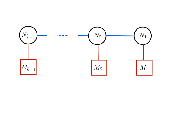
Figure 1: A linear quiver: circles denote gauge group factors $U(N_{j})$, while squares stand for hypermultiplets in the fundamental representation of the corresponding factor group. There is also one bi-fundamental hypermultiplet for each neighbouring pair of gauge group factors, denoted by a single blue line.

Any two partitions $\rho$ and $\hat{\rho}$ of $N$ determine completely the gauge theory data $\{N_{j},M_{j}\}$. Two useful parametrizations of the partition $\rho$ are given by

$$\rho:\qquad~{}N = l_{1}+\ldots+l_{k}$$ (2.2)

$$= \underbrace{1+\ldots+1}_{M_{1}}\,+\,\underbrace{2+\ldots+2}_{M_{2}}\,+\,\ldots+\ldots\ .$$

Here the $l_{i}$ are positive non-increasing integers, $l_{1}\geq l_{2}\ldots\geq l_{k}>0$, while $M_{l}$ is the number of times the integer $l$ occurs in this decomposition. The $M_{l}$ are thus zero or positive, and they obey the sum rule $\sum lM_{l}=N$. One can associate to $\rho$ a Young tableau whose rows have lengths $l_{1},\ldots,l_{k}$. The same parametrizations can also be used for the partition $\hat{\rho}$,

$$\hat{\rho}:\qquad~{}N = \hat{l}_{1}+\ldots+\hat{l}_{\hat{k}}$$ (2.3)

$$= \underbrace{1+\ldots+1}_{\hat{M}_{1}}\,+\,\underbrace{2+\ldots+2}_{\hat{M}_{2}}\,+\,\ldots+\ldots\,.$$

With this choice of “coordinates”, $M_{j}$ is precisely the number of hypermultiplets in the fundamental representation of the $j$th group factor, while the rank of each gauge group factor is given by

$$N_{1}=k-\hat{l}_{1}\,,\qquad{\rm and}\qquad N_{j}=N_{j-1}+m_{j}-\hat{l}_{j}\qquad{\rm for}\qquad j=2,\cdots\hat{k}-1\ .$$ (2.4)

Here $m_{l}$ counts the number of terms that are equal or bigger than $l$ in the first line of equation (2.2). Thus $m_{1}=k$, and $m_{l+1}=m_{l}-M_{l}$. As can be easily seen, the $m_{l}$ are a non-increasing sequence of positive integers defining the partition $\rho^{T}$, whose Young tableau is the transpose of the Young tableau of the partition $\rho$.

The condition (1.1) on the two Young tableaux is a short-hand notation for the following set of strict inequalities:

$$\rho^{T}>\hat{\rho}\ \ \Longleftrightarrow\ \ \sum_{s=1}^{i}m_{s}\ >\ \sum_{s=1}^{i}\hat{l}_{s}\qquad\forall i=1,\ldots,l_{1}\,.$$ (2.5)

Stated in words, the total number of boxes in the first $i$ rows of the Young tableau $\rho^{T}$ is strictly larger than the same number in the tableau $\hat{\rho}$. Note that the tableau $\rho^{T}$ has $l_{1}$ rows, while the number of rows in $\hat{\rho}$ is $\hat{k}$. Since the two tableaux have the same total number of boxes, namely $N$, it follows automatically that $\hat{\rho}$ must have more rows than $\rho^{T}$, i.e. that $\hat{k}>l_{1}$.

As can be seen from equation (2.4), the condition (2.5) is equivalent to requiring that the rank $N_{i}$, for each $U(N_{i})$ gauge group factor in the quiver diagram be a positive integer. This condition also implies that $M_{l}=0$ for $l\geq\hat{k}$, so that there are no hypermultiplets corresponding to empty gauge-group factors. Thus $\rho^{T}>\hat{\rho}$ is necessary in order for the linear quiver associated to the triplet $(\rho,\hat{\rho},N)$ to make sense. Note that if one of the inequalities in (2.5) is replaced by an equality, the quiver breaks into two disconnected components. What Gaiotto and Witten have conjectured is that all these quiver gauge theories flow to non-trivial infrared fixed points [2]. The existence of the dual gravity solutions, presented in the following section, is indirect evidence in favor of this conjecture.

The gauge theories $T^{\rho}_{\hat{\rho}}(SU(N))$ have both a Coulomb and a Higgs branch of vacua parametrized, respectively, by the vector-multiplet and hypermultiplet expectation values. Remarkably, the gauge theory $T_{\rho}^{\hat{\rho}}(SU(N))$ has precisely the same moduli space of vacua as $T^{\rho}_{\hat{\rho}}(SU(N))$, but with the role of Coulomb and Higgs branches exchanged. Since $\rho^{T}>\hat{\rho}$ implies $\hat{\rho}^{T}>\rho$ and vice-versa [3], both $T^{\rho}_{\hat{\rho}}(SU(N))$ and $T_{\rho}^{\hat{\rho}}(SU(N))$ are expected to flow to an infrared superconformal field theory. In fact, $T^{\rho}_{\hat{\rho}}(SU(N))$ and $T_{\rho}^{\hat{\rho}}(SU(N))$ are believed to flow to the same superconformal field theory, at the intersection of the Higgs and the Coulomb branch. This is a prime example of three dimensional mirror symmetry [14], which can be attributed to the S-duality of the underlying type-IIB string theory, where these theories admit an elegant brane realization (see section 2.1).

An important guide in the construction of the dual geometries is that they must realize the global symmetries of these superconformal field theories. The three dimensional ${\mathcal{N}}=4$ superconformal algebra is $OSp(4|4)$. The bosonic symmetries include $SO(2,3)$, the conformal group in three dimensions, and $SO(4)\simeq SU(2)_{1}\times SU(2)_{2}$, which is the associated $R$-symmetry.

These superconformal field theories also exhibit, however, a rich pattern of additional global symmetries, that depend on $\rho$ and $\hat{\rho}$ – the data that determines as we just saw the (mirror pair of) ultraviolet gauge theories whose infrared limit we want to describe. In a given ultraviolet Lagrangian description, only part of the fixed-point symmetry is manifest. This is the one acting on the Higgs branch of the theory. From the symmetry acting on the Coulomb branch, only the maximal abelian subgroup is in general manifest in the Lagrangian description. Fortunately, the Coulomb branch symmetry of a given theory – say $T^{\rho}_{\hat{\rho}}(SU(N))$ – can be read from the Higgs branch symmetry of its mirror, that is $T_{\rho}^{\hat{\rho}}(SU(N))$. Thus, the full global symmetry at the superconformal point is believed to be $H_{\rho}\times H_{\hat{\rho}}$, where

$$H_{\rho}=\prod_{i}U(M_{i})\qquad{\rm and}\qquad H_{\hat{\rho}}=\prod_{i}U(\hat{M}_{i})\,.$$ (2.6)

This is the symmetry that rotates the fundamental hypermultiplets of each gauge group factor in the quiver diagram of $T^{\rho}_{\hat{\rho}}(SU(N))$ and its mirror.

2.1 Brane construction of linear quivers

The gauge theories $T^{\rho}_{\hat{\rho}}(SU(N))$ can be realized as low-energy limits of certain type-IIB brane configurations on the interval. Indeed this is how these theories were introduced in the first place. We will here sketch the salient features of these brane constructions, and refer the reader to [2] and [15] for further explanations and more references. The basic setup consists of:
  - a set of $k$ D5-branes spanning the dimensions (012456),
  - a set of $\hat{k}$ NS5-branes spanning the dimensions (012789), and
  - a set of D3-branes stretched among the five-branes along (0123).
Such configurations preserve 1/4 of the supersymmetries of type-IIB string theory, which correspond to the three dimensional ${\mathcal{N}}=4$ Poincaré supersymmetries of $T^{\rho}_{\hat{\rho}}(SU(N))$. The brane configuration has a manifest $SU(2)_{1}\times SU(2)_{2}$ rotation symmetry in the (456) and (789) dimensions, which gets identified with the $R$-symmetry of $T^{\rho}_{\hat{\rho}}(SU(N))$, and also coincides with the $R$-symmetry of the infrared superconformal field theory. The vector multiplets live on the D3-branes, and since these have finite extent on the interval along the $x^{3}$ dimension, they give rise at large distances to a three dimensional gauge theory. Hypermultiplets arise from open strings stretching between the D3-branes and the D5-branes, or between two stacks of D3-branes ending on the same NS5-brane from the left and right. The five-branes are localized in the interval direction spanned by $x^{3}$.

In the infrared limit, the distance between the five-branes becomes irrelevant, and the gauge theory is expected to flow, under suitable conditions, to a three dimensional (in general strongly-interacting) theory with superconformal symmetry $OSp(4|4)$. The relevant data in the brane construction is the ordering of the five-branes along the $x^{3}$ segment, as well as the net number of D3-branes ending on each one of them. This data is actually redundant, since rearrangements of the five-branes change the phase of the gauge theory, but presumably not its superconformal (infrared) limit. The truly relevant data, besides the total numbers $k$ and $\hat{k}$ of D5- and NS5-branes of each kind, are the linking numbers associated with each five-brane separately [15]. These can be defined as follows:

$$l_{i} = -n_{i}+R_{i}^{\rm NS5}\ \ \ \ (i=1,\cdots k)$$

$$\hat{l}_{j} = \hat{n}_{j}+L^{\rm D5}_{j}\ \ \ \ (j=1,\cdots\hat{k})\,,$$ (2.7)

where $n_{i}$ is the number of D3-branes ending on the $i$th D5-brane from the right minus the number of D3-branes ending on it from the left, $\hat{n}_{j}$ is the same quantity for the $j$th NS5-brane, $R_{i}^{\rm NS5}$ is the number of NS5-branes lying to the right of the $i$th D5-brane, and $L^{\rm D5}_{j}$ is the number of D5-branes lying to the left of the $j$th NS5-brane. The linking numbers are invariant under five-brane moves, because when a D5 moves past a NS5 in the direction from left to right, a D3-brane stretching between the two is created. Consistency requires that the inverse move should result in the annihilation of a stretched D3-brane (or the creation of an anti-D3 brane).

The configurations of interest [2] which realize $T^{\rho}_{\hat{\rho}}(SU(N))$ can be depicted as $N$ D3-branes in the middle ending on the left on a collection of NS5-branes and on the right on a collection of D5-branes. Each D3-brane terminates on some NS5-brane on the left, and on some D5-brane on the right (see figure 2). This implies that the number of D3-branes that terminate on each five-brane is precisely the linking number defined in (2.1), and that furthermore

$$N\,=\,l_{1}+\ldots+l_{k}\,=\,\hat{l}_{1}+\ldots+\hat{l}_{\hat{k}}\ .$$ (2.8)

These are the two partitions of $N$, $\rho$ and $\hat{\rho}$, that label the theory $T^{\rho}_{\hat{\rho}}(SU(N))$. The partition $\hat{\rho}$ encodes the linking numbers of the NS5-branes, while $\rho$ encodes the linking number of the D5-branes. $S$-duality of the type-IIB string theory exchanges the two type of five-branes, and thus the two partitions. Therefore, the S-dual brane configuration realizes the mirror theory $T_{\rho}^{\hat{\rho}}(SU(N))$, so that S-duality acts as mirror symmetry in the gauge theory.

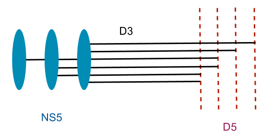
Figure 2: A brane configuration with $N=6$, $\rho=(2,2,1,1)$ and $\hat{\rho}=(3,2,1)$ .

Since five-branes of the same kind are not connected with D3-branes, they can be moved freely past each other, so their relative order is irrelevant in the infrared limit. We will adopt the convention that the linking numbers of the NS5-branes are non-decreasing from left to right, and that the same holds for the D5-branes from right to left. Thus $l_{1}\geq l_{2}\cdots\geq l_{k}$ and $\hat{l}_{1}\geq\hat{l}_{2}\cdots\geq\hat{l}_{\hat{k}}$, where $i=1$ and $j=1$ are the innermost five-branes, while $i=k$ and $j=\hat{k}$ are the outermost ones. As was already explained, it is convenient to associate to $\rho$ a Young tableau whose rows have $l_{1},\cdots,l_{k}\,$ boxes, and likewise for $\hat{\rho}$.

We are now ready to explain the condition that forces the ordering (2.5) of the Young tableaux. To understand the origin of this constraint, let us try to rearrange all D5-branes so that no D3-branes terminate on them at all, i.e. so that their linking numbers are equal to the number of NS5-branes that lie on their right. This is the configuration in which the field content of the quiver gauge theory is most easy to read (see figure 3). The argument that we will now explain shows, in a nutshell, that unbroken supersymmetry requires the weaker condition $\hat{\rho}^{T}\geq\rho$, or equivalently $\rho^{T}\geq\hat{\rho}$. However, when the inequality is saturated the corresponding quiver gauge theory breaks down to pieces that flow to non-interacting superconformal theories in the infrared.

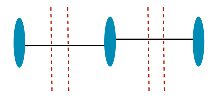
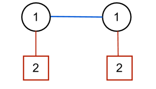
Figure 3: On the left, the brane construction of figure 2 after moving the D5-branes in the way described in the text. On the right the quiver diagram describing the corresponding supersymmetric gauge theory.

To see why, start moving the innermost D5-brane towards the left. Each time it crosses a NS5, one of the D3-branes ending on it is destroyed. If $l_{1}<\hat{k}$ the process stops when there are no more D3-branes terminating on our D5-brane, i.e. after having crossed all but $\hat{k}-l_{1}$ of the NS5-branes. What if $l_{1}>\hat{k}$? In this case, after moving $\hat{k}-1$ steps, our D5-brane will be attached to the outermost NS5-brane by more than one stretched D3-branes. This is forbidden by the s-rule, which states that such a gauge theory would have no supersymmetric ground states [15]. The marginal case $l_{1}=\hat{k}$ is not forbidden by the $s$-rule. In this case, however, in the final step the D5-brane will be detached from the rest of the quiver, and the infrared superconformal theory could be described by a partition $\rho^{\prime}$ whose Young tableau has one less row than our original partition $\rho$. Since we only want to characterize distinct superconformal theories, we should not count separately $\rho$ and $\rho^{\prime}$. By convention we only keep the partitions with the minimal number of rows. This implies the additional condition of $\hat{\rho}^{T}>\rho$ namely $\hat{l}_{1}<k$, which ensures that no NS5-branes are detached to the right of the quiver.

Assume then that $l_{1}<\hat{k}$, and try now to rearrange the second innermost D5. The first two D5-branes have a total of $l_{1}+l_{2}$ D3s ending on them. At most $\hat{M}_{1}=\hat{m}_{1}-\hat{m}_{2}$ of these can terminate on NS5-branes that have only a single D3-brane attached. [Recall the definition of $\hat{m}_{l}$ as the number of NS5-branes with at least $l$ D3-branes attached, or equivalently as the partition corresponding to the transposed Young tableau $\hat{\rho}^{T}$]. There remain, therefore, at least $l_{1}+l_{2}-(\hat{m}_{1}-\hat{m}_{2})$ D3-branes, that must be attached to the remaining NS5-branes. Unless

$$2\hat{m}_{2}\geq l_{1}+l_{2}-(\hat{m}_{1}-\hat{m}_{2})\ \Longleftrightarrow\ \hat{m}_{1}+\hat{m}_{2}\geq l_{1}+l_{2}\ ,$$ (2.9)

some D5/NS5 pairs would be attached by more than one D3-brane, thereby violating the $s$-rule. Thus supersymmetry requires that (2.9) hold. Furthermore, In the marginal case $\hat{m}_{1}+\hat{m}_{2}=l_{1}+l_{2}$, the quiver gauge theory can be again reduced, i.e. it breaks down to separate pieces that flow to decoupled superconformal theories in the infrared. This can be shown by first moving both D5-branes $\hat{m}_{2}$ steps, so that they enter the region of singly-attached NS5-branes. The latter are furthermore all attached to these two D5-branes, and to nothing else. It is then easy to see that the remaining $\hat{m}_{1}-\hat{m}_{2}$ moves will necessarily break up the quiver.

We now state the general result, which can be proved by induction with the above logic. By slight abuse of notation, we write $\rho^{T}\geq\hat{\rho}$ for the weaker form of (2.5) in which the total number of boxes up to the $i$th row must be greater or equal on the two sides. Then the brane rearrangement argument shows that:

$${\rm supersymmetry}\,\Longleftrightarrow\,\hat{\rho}^{T}\geq\rho\ ,\ \ \ {\rm and}\ \ \ {\rm irreducibility}\,\Longleftrightarrow\,\hat{\rho}^{T}>\rho\ .$$ (2.10)

When the strong form of the constraint is satisfied, the configuration after completing all rearrangements of D5-branes consists of a connected linear chain of $\hat{k}$ NS5-branes, attached in pairs by $N_{j}$ D3-branes. The D5-branes intersect, but are detached from the D3-branes. The corresponding gauge theory data can be read easily from this configuration: there is one $U(N_{j})$ gauge group factor for every set of stretched D3-branes, one hypermultiplet in the bifundamental representation for each adjacent pair, and one hypermultiplet in the fundamental representation of the corresonding gauge group for each D5-brane. The final result agrees precisely with the gauge theory content of $T^{\rho}_{\hat{\rho}}(SU(N))$ described in the previous subsection.

3 The ${\rm AdS}_{4}\ltimes K$ Supergravity Solutions

We will now derive the gravitational backgrounds dual to the superconformal field theories labeled by $(\rho,\hat{\rho})$ described in the previous section, as special limits of the type IIB-supergravity solutions found in [4, 5]. These were analyzed as candidate backgrounds for gravity localization in [9], whose conventions and notation we adopt. The main new result in this section is the existence of a smooth limit in which the asymptotic ${\rm AdS}_{5}\times{\rm S}^{5}$ regions of the solutions of [4, 5] are truncated away, and the space transverse to the ${\rm AdS}_{4}$ slices is compactified to $K$.

3.1 Local solutions: General form

For the reader’s convenience we collect here the formulae describing the general form of the solutions of [4, 5]. These solutions are fibrations of ${\rm AdS}_{4}\times{\rm S}^{2}\times{\rm S}^{2}$ over a base space which is a Riemann surface $\Sigma$ with the topology of a disk. The general discussion of these solutions [5] is most convenient with a choice of complex coordinate that varies over the upper-half plane, but for our purposes here we prefer to use a coordinate that varies over the infinite strip:

$$\Sigma\equiv\{z\in\mathbb{C}\,|\,0\leq{\rm Im}z\leq{\pi\over 2}\}\ .$$

The solutions have a manifest ${SO}(2,3)\times{SU}(2)_{1}\times{SU}(2)_{2}$ symmetry realized on the fibers, which combined with the sixteen super(conformal) symmetries of the solutions, give a bulk realization of the three dimensional $OSp(4|4)$ supeconformal algebra. The solutions are completely specified by two functions $h_{1}(z,\bar{z})$ and $h_{2}(z,\bar{z})$ which are real harmonic and regular inside $\Sigma$, and which obey the boundary conditions (here $\partial_{\perp}$ is the normal derivative):

$$h_{1}=\partial_{\perp}h_{2}=0\hskip 14.22636pt{\rm for}\hskip 14.22636pt{\rm Im}z=0\ ,\hskip 28.45274pth_{2}=\partial_{\perp}h_{1}=0\hskip 14.22636pt{\rm for}\hskip 14.22636pt{\rm Im}z={\pi\over 2}\ .$$ (3.1)

In writing down the solutions one also needs the dual harmonic functions, which are defined by the following relations

$$h_{1}=-i({\cal A}_{1}-\bar{\cal A}_{1})\qquad\rightarrow\qquad h_{1}^{D}={\cal A}_{1}+\bar{\cal A}_{1}\ ,$$

$$h_{2}={\cal A}_{2}+\bar{\cal A}_{2}\qquad\rightarrow\qquad h_{2}^{D}=i({\cal A}_{2}-\bar{\cal A}_{2})\ .$$ (3.2)

The dual functions are in general ambiguous. These ambiguities will have, however, a simple physical interpretation, as gauge transformations of the RR and NSNS 2-form gauge potentials (see section 4). Besides the dual functions, it is also convenient to define the following combinations of $h_{1}$, $h_{2}$, and of their first derivatives (here $\partial=\partial/\partial z,\bar{\partial}=\partial/\partial\bar{z}$) :

$$W = \partial h_{1}\bar{\partial}h_{2}+\bar{\partial}h_{1}\partial h_{2}=\partial\bar{\partial}(h_{1}h_{2})\ ,$$

$$N_{1} = 2h_{1}h_{2}|\partial h_{1}|^{2}-h_{1}^{2}W\ ,$$

$$N_{2} = 2h_{1}h_{2}|\partial h_{2}|^{2}-h_{2}^{2}W\ .$$ (3.3)

Now in the conventions of [9] the solution reads:

$$\underline{\rm Metric}:\qquad ds^{2}=f_{4}^{2}ds_{{\rm AdS}_{4}}^{2}+f_{1}^{2}ds_{{\rm S}_{1}^{2}}^{2}+f_{2}^{2}ds_{{\rm S}_{2}^{2}}^{2}+4\rho^{2}dzd\bar{z}\ ,$$ (3.4)

where

$$f_{4}^{8} = 16\,{N_{1}N_{2}\over W^{2}}\ ,\qquad\qquad\rho^{8}={N_{1}N_{2}W^{2}\over h_{1}^{4}h_{2}^{4}}\ ,$$

$$f_{1}^{8} = 16\,h_{1}^{8}{N_{2}W^{2}\over N_{1}^{3}}\ ,\qquad\qquad f_{2}^{8}=16\,h_{2}^{8}{N_{1}W^{2}\over N_{2}^{3}}\ ,$$ (3.5)

and the ${\rm AdS}_{4}$ and 2-sphere metrics are normalized to unit radius;

$$\hskip-170.71652pt\underline{\rm Dilaton}:\qquad e^{4\phi}={N_{2}\over N_{1}}\ ;$$ (3.6)

$$\underline{\rm 3{\rm-}forms}:\qquad H_{(3)}=\omega^{\,45}\wedge db_{1}\qquad{\rm and}\qquad\,F_{(3)}=\omega^{\,67}\wedge db_{2}\ ,$$ (3.7)

where $H_{(3)}$ and $F_{(3)}$ are the NS/NS and R/R  3-form field strengths, $\omega^{\,45}$ and $\omega^{\,67}$ are the volume forms of the unit-radius spheres ${\rm S}_{1}^{2}$ and ${\rm S}_{2}^{2}$, and

$$b_{1} = 2ih_{1}{h_{1}h_{2}(\partial h_{1}\bar{\partial}h_{2}-\bar{\partial}h_{1}\partial h_{2})\over N_{1}}+2h_{2}^{D}\ ,$$

$$b_{2} = 2ih_{2}{h_{1}h_{2}(\partial h_{1}\bar{\partial}h_{2}-\bar{\partial}h_{1}\partial h_{2})\over N_{2}}-2h_{1}^{D}\ ;$$ (3.8)

$$\hskip-17.07182pt\underline{\rm 5{\rm-}form}:\qquad F_{(5)}=-4\,f_{4}^{4}\,\omega^{\,0123}\wedge{\cal F}+4\,f_{1}^{2}f_{2}^{2}\,\omega^{\,45}\wedge\omega^{\,67}\wedge(*_{2}{\cal F})\ ,$$ (3.9)

where $\omega^{\,0123}$ is the volume form of the unit-radius ${\rm AdS}_{4}$, ${\cal F}$ is a 1-form on $\Sigma$ with the property that $f_{4}^{\,4}{\cal F}$ is closed, and $*_{2}$ denotes Poincaré duality with respect to the $\Sigma$ metric. The explicit expression for ${\cal F}$ is given by

$$f_{4}^{\,4}{\cal F}=dj_{1}\ \qquad{\rm with}\qquad j_{1}=3{\cal C}+3\bar{\cal C}-3{\cal D}+i\frac{h_{1}h_{2}}{W}\,(\partial h_{1}\bar{\partial}h_{2}-\bar{\partial}h_{1}\partial h_{2})\ ,$$ (3.10)

where ${\cal C}$ is defined by the relation $\partial{\cal C}={\cal A}_{1}\partial{\cal A}_{2}-{\cal A}_{2}\partial{\cal A}_{1}$ while ${\cal D}=\bar{\cal A}_{1}{\cal A}_{2}+{\cal A}_{1}\bar{\cal A}_{2}$.

The above set of expressions gives the local form of the general solution for the ansatz of references [4, 5]. These expressions are invariant under conformal transformations of the coordinate $z$, which map, however, in general $\Sigma$ to a different disk-like domain of the complex plane.

3.2 Asymptotic $AdS_{5}\times S^{5}$ regions and five-branes

The simplest solution with all necessary ingredients for our purposes here corresponds to the following choice of real harmonic functions: [5, 9]

$$h_{1} = \,\left[-i\alpha\,{\rm sinh}(z-\beta)-\gamma\,{\rm ln}\left({\rm tanh}\left({i\pi\over 4}-{z-\delta\over 2}\right)\right)\right]+{\rm c.c.}\ ,$$

$$h_{2} = \,\left[\hat{\alpha}\,{\rm cosh}(z-\hat{\beta})-\hat{\gamma}\,{\rm ln}\left({\rm tanh}\left({z-\hat{\delta}\over 2}\right)\right)\right]+{\rm c.c.}\ .$$ (3.11)

The parameters ($\alpha,\beta,\gamma,\delta$) and ($\hat{\alpha},\hat{\beta},\hat{\gamma},\hat{\delta}$) are all real. The only other condition on this set of parameters, explained in [5], is that $\alpha\gamma$ and $\hat{\alpha}\hat{\gamma}$ must be non-negative. If not, the solution has curvature singularities supported on a one-dimensional curve in the interior of $\Sigma$, which have no interpretation in string theory.

This solution describes the near-horizon geometry of stacks of intersecting D3-branes, NS5-branes and D5-branes. The setup preserves the same super-Poincaré and $R$ symmetries as the brane constructions considered in our discussion of linear quiver gauge theories in section 2. Flipping the sign of $\alpha$ and $\gamma$ amounts to trading the D3-branes and D5-branes for anti-branes. Without loss of generality, we will thus assume from now on that $\alpha,\gamma,\hat{\alpha},\hat{\gamma}$ are all non-negative.

Let us describe the main features of the above background. In the two regions $Re(z)\rightarrow\pm\infty$ it approaches asymptotically the $AdS_{5}\times S^{5}$ solution, with the values of the radius and the dilaton given by: [9]

$$L_{\pm}^{4}\,=\,16|\alpha^{\pm}\hat{\alpha}^{\pm}|\,{\rm cosh}(\beta^{\pm}-\hat{\beta}^{\pm})\qquad{\rm and}\qquad e^{2\phi_{\pm}}=\left|{\hat{\alpha}^{\pm}\over\alpha^{\pm}}\right|e^{\pm(\beta^{\pm}-\hat{\beta}^{\pm})}\ ,$$ (3.12)

where $\alpha^{\pm}$ and $\beta^{\pm}$ are given by:

$$\alpha^{\pm}=\alpha\,\sqrt{1+{4\gamma\over\alpha}e^{\pm(\delta-\beta)}}\ ,\qquad e^{\beta^{\pm}}=e^{\beta}\,\left(1+{4\gamma\over\alpha}e^{\pm(\delta-\beta)}\right)^{\pm 1/2}\ ,$$ (3.13)

with similar expressions holding for the hatted quantities $\hat{\alpha}^{\pm}$ and $\hat{\beta}^{\pm}$. In the limit $\gamma=\hat{\gamma}=0$, the solution becomes the supersymmetric Janus domain wall, in which the dilaton field varies from one asymptotic $AdS_{5}\times S^{5}$ region to the other. Setting in addition $\beta=\hat{\beta}=0$, gives the global $AdS_{5}\times S^{5}$ solution with radius $L^{4}=16\,\alpha\hat{\alpha}$ and a constant dilaton given by $e^{2\phi}=\hat{\alpha}/\alpha$.

The other important feature of the above solution is the presence of singularities on the boundary of the strip, namely at $z=i\frac{\pi}{2}+\delta$ and $z=\hat{\delta}$. These are associated with the non-trivial 3-cycles in the geometry. The solutions that we consider have the property that on the lower boundary of $\Sigma$ the two sphere $S_{1}^{2}$ shrinks to zero size smoothly (there is no conical singularity) and on the upper boundary of $\Sigma$ the two sphere $S_{2}^{2}$ shrinks to zero size smoothly. Therefore, with the exception of the singular points $z=i\frac{\pi}{2}+\delta$ and $z=\hat{\delta}$, the rest of the boundary of the strip corresponds to interior points of the ten dimensional geometry. Now consider a small open curve $I$ in $\Sigma$, which surrounds the singularity at $z=\hat{\delta}$ and ends on the ${\rm Im}(z)$=0 axis, where the 2-sphere $S_{1}^{2}$ shrinks to zero. Then $I\times S^{2}_{1}$ is a non-contractible 3-cycle which is, furthermore, threaded by non-vanishing $H_{(3)}$ flux, as can be checked with the help of the expressions (3.7) and (3.1). This flux signals that the local geometry describes a stack of NS5-branes, whose total charge is proportional to $\hat{\gamma}$. Likewise, the region near $z=i\frac{\pi}{2}+\delta$ describes a stack of D5-branes, with total charge proportional to the parameter $\gamma$ (see section 4). Note that at these singularities the dilaton field diverges, as expected near the location of five-branes.

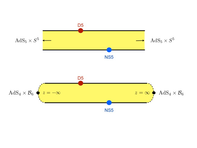
Figure 4: The four asymptotic regions of the solution (3.2): near $z\simeq\pm\infty$ the geometry asymptotes to $AdS_{5}\times S^{5}$, while the singularities on the lower and the upper strip boundary describe stacks of NS5 branes and D5 branes. Taking $\alpha$ and $\hat{\alpha}$ to zero replaces the $AdS_{5}\times S^{5}$ regions by smooth caps homeomorphic to $AdS_{4}$ times a 6-dimensional ball.

3.3 Closing the $AdS_{5}\times S^{5}$ regions

As explained in the last subsection, the $z\to\pm\infty$ regions of the strip describe regions of the 10-dimensional solution that approach $AdS_{5}\times S^{5}$, with the radii given by the expressions (3.12) and (3.13). These radii vanish if we take $\alpha$ and $\hat{\alpha}$ to zero, while keeping the other parameters of the solution fixed. Interestingly enough the limit is smooth: the asymptotic $AdS_{5}\times S^{5}$ regions are replaced in this limit by regions that are homeomorphic to $AdS_{4}\times{\cal B}_{6}$, where ${\cal B}_{6}$ is the 6-dimensional ball. This is depicted schematically in the lower part of figure 4.

Let us be a little more explicit. The limiting geometry is described by the two harmonic functions:

$$h_{1}=\,-\gamma\,{\rm ln}\,{\rm tanh}\left({i\pi\over 4}-{z-\delta\over 2}\right)+{\rm c.c.}\ ;\ \ h_{2}=\,-\hat{\gamma}\,{\rm ln}\,{\rm tanh}\left({z-\hat{\delta}\over 2}\right)+{\rm c.c.}\ .$$ (3.14)

Inserting these two functions in the expression (3.4) for the metric, and making the following change of coordinates:

$$r^{2}=2(e^{2\delta}+e^{2\hat{\delta}})\,e^{-2x}\qquad{\rm where}\qquad z=x+iy\ ,$$

gives in the limit $x\to\infty$:

$$ds^{2}\simeq L^{2}\,\Big{[}ds^{2}_{AdS_{4}}\,+\,dr^{2}\,+\,r^{2}\left(\sin^{2}y\,ds^{2}_{S^{2}_{1}}\,+\,\cos^{2}y\,ds^{2}_{S^{2}_{2}}\,+\,dy^{2}\right)\Big{]}\,$$ (3.15)

with

$$L^{4}={16\,{\gamma\hat{\gamma}}\over{\rm cosh}(\delta-\hat{\delta})}\ .$$ (3.16)

This is locally $AdS_{4}\times\mathbb{R}^{6}$, which shows that the $z\simeq\infty$ region becomes a regular interior region of the 10-dimensional geometry, as advertized. The Ricci scalar in the $x\to\infty$ limit asymptotes to ${\cal R}\simeq 8/L^{2}$, while the dilaton and the $p$-form fields are also finite. The region $x\to-\infty$ can be analyzed similarly; it is in fact sufficient to flip the signs of $\delta$ and $\hat{\delta}$ in the above expressions.

The complete metric defined by the harmonic functions (3.14) describes a warped product $AdS_{4}\ltimes K$, where $K$ is a compact 6-dimensional manifold with admissible singularities at the location of the five-branes. Notice that the overall scale of the metric is proportional to $\sqrt{\gamma\hat{\gamma}}$, so that both types of five-brane stacks are required for a regular solution. This is our first example of a background which is the gravity dual of the ${\mathcal{N}}=4$ superconformal theories labeled by the pair of partitions $(\rho,\hat{\rho})$. As will become clear in the following sections, this first example corresponds to two equipartitions of the D3-branes, $N=lM_{l}=\hat{l}\hat{M}_{\hat{l}}$. The simplest possible partitions

$$\rho=\hat{\rho}:\qquad N=\underbrace{1+1+\ldots+1}_{N}\,$$ (3.17)

are obtained in the special case $\gamma=\hat{\gamma}$ and $\hat{\delta}-\delta=\ln\tan{\pi\over 2N}$. The superconformal theory (and quiver gauge theories) corresponding to this simplest choice of partitions is sometimes denoted by just $T(SU(N))$. Notice that for this example the gauge theory is identical to its mirror.

3.4 Many stacks of five-branes

It is easy to generalize the above solution so as to include many singularities which will describe the asymptotic regions of different stacks of D5-branes and NS5-branes. The corresponding harmonic functions are given by

$$h_{1} = \left[-i\alpha\sinh(z-\beta)-\sum_{a=1}^{q}\gamma_{a}\ln\left(\tanh\left(\frac{i\pi}{4}-\frac{z-\delta_{a}}{2}\right)\right)\right]+c.c.$$

$$h_{2} = \left[\hat{\alpha}\cosh(z-\hat{\beta})-\sum_{b=1}^{\hat{q}}\hat{\gamma}_{b}\ln\left(\tanh\left(\frac{z-\hat{\delta}_{b}}{2}\right)\right)\right]+c.c.$$ (3.18)

with $\delta_{1}<\delta_{2}<...<\delta_{q}$ and $\hat{\delta}_{1}>\hat{\delta}_{2}>...>\hat{\delta}_{\hat{q}}$.

The solution described by these harmonic functions contains two asymptotic $AdS_{5}\times S^{5}$ regions, $q$ singularities on the upper boundary of $\Sigma$ corresponding to $q$ stacks of D5-branes, and $\hat{q}$ singularities on the lower boundary of $\Sigma$ corresponding to $\hat{q}$ stacks of NS5-branes. The $a^{th}$ stack of D5-branes is located at $z=i\frac{\pi}{2}+\delta_{a}$ and contains a number of D5-branes proportional to $\gamma_{a}$, while the $b^{th}$ stack of NS5-branes is located at $z=\hat{\delta}_{b}$ and contains a number of NS5-branes proportional to $\hat{\gamma}_{b}$. Note that we choose to label the singularities on the upper boundary of the strip from left to right, and on the lower boundary from right to left. This choice will prove convenient when identifying the parameters of the solution with the data of the dual superconformal field theory, in section 5.

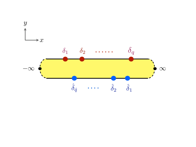
Figure 5: The infinite strip with several singularities, corresponding to many different stacks of five-branes. The positions of these singularities along the real axis are related to the data of the dual superconformal field theory, in a way that will be detailed in section 4.

The solution (3.4) describes the near-horizon geometry of a brane construction that contains D3-branes stretched between the two asymptotic regions, between the asymptotic regions and the stacks of five-branes, and between the D5- and NS5-brane stacks. This can be seen from the calculation of the 5-form flux that enters in the various asymptotic regions, as will be detailed in the following section.

We may now proceed as before to close the two asymptotic $AdS_{5}\times S^{5}$ regions by setting $\alpha=\hat{\alpha}=0$. The resulting harmonic functions are :

$$h_{1} = -\sum_{i=a}^{q}\gamma_{a}\ln\left(\tanh\left(\frac{i\pi}{4}-\frac{z-\delta_{a}}{2}\right)\right)+c.c.$$

$$h_{2} = -\sum_{b=1}^{\hat{q}}\hat{\gamma}_{b}\ln\left(\tanh\left(\frac{z-\hat{\delta}_{b}}{2}\right)\right)+c.c.$$ (3.19)

In this class of solutions the manifold is of the type $AdS_{4}\ltimes K$ where the $AdS_{4}$ is fibered over the compact six-dimensional manifold $K$. The closure of the $AdS_{5}\times S^{5}$ regions is smooth, and the points at infinity become interior points (locally $AdS_{4}\times\mathbb{R}^{6}$), as explained in the previous subsection. In the rest of this paper we will focus on this class of type-IIB supergravity solutions, and propose a precise correspondence with the three dimensional ${\mathcal{N}}=4$ superconformal field theories labeled by the two partitions $(\rho,\hat{\rho})$, and discussed in section 2.

We should mention here as a side remark that it is also possible to close only one asymptotic $AdS_{5}\times S^{5}$ region, by taking an appropriate limit of parameters. In this case it seems natural, even if we didn’t look at it in detail, that one can derive a similar correspondence with four dimensional ${\mathcal{N}}=4$ super-Yang-Mills on half-space with suitable half-supersymmetric conditions imposed at the boundary. This type of boundary conditions has been studied in detail in [8, 2]. The supergravity analysis of this case has appeared in the recent reference [13], which has some partial overlap with our work. The possibility of closing off an $AdS_{5}\times S^{5}$ region has been, in particular, also observed in this reference. Here we close off both $AdS_{5}\times S^{5}$ regions, and end up with $AdS_{4}\ltimes K$ backgrounds dual to three dimensional superconformal field theories, rather than ${\mathcal{N}}=4$ super-Yang-Mills in half-space. Another interesting class of limits are factorization limits of the five-brane singularities; these will be discussed briefly near the end of this paper.

4 Brane Charges and Quantization

In order to discuss the precise correspondence between the supergravity solutions of section 3 and the superconformal field theories to which $T^{\rho}_{\hat{\rho}}(SU(N))$ and $T_{\rho}^{\hat{\rho}}(SU(N))$ flow in the infrared, we must first compute the charges contained in the supergravity backgrounds. The definition of the amount of D3-brane charge dissolved into the D5-brane and NS5-brane stacks is subtle and suffers from a well known ambiguity. In particular, the so-called “Page charge” (which is quantized and localized) transforms under large gauge transformations of the two-form gauge potentials $B_{2}$ and $C_{2}$ (see [18] for a nice discussion of the issue). We will give below a physical interpretation of this gauge ambiguity in terms of the Hanany-Witten effect [15].

Let us start then by introducing the non-trivial 3- and 5-cycles which support the D3-brane, D5-brane and NS5-brane charges:

• ${\cal C}^{a}_{3}$: are defined by the fibration of $S_{2}^{2}$ over a line segment in $\Sigma$ which ends on the upper boundary of the strip and encloses the point $\delta_{a}$. Note that $h_{2}=0\Rightarrow f_{2}=0$ on the upper boundary, so that ${\cal C}^{a}_{3}$ is topologically also a 3-sphere.

• $\hat{\cal C}^{b}_{3}$: are defined by the fibration of $S_{1}^{2}$ over a line segment in $\Sigma$ which ends on the lower boundary and encloses the point $\hat{\delta}_{b}$. Note that $h_{1}=0\Rightarrow f_{1}=0$ on the lower boundary so that $\hat{\cal C}^{b}_{3}$ is topologically a 3-sphere.

• ${\cal C}^{a}_{5}$: is defined by the warped product $S_{1}^{2}\ltimes{\cal C}^{a}_{3}$ and is topologically an $S^{3}\times S^{2}$.

• $\hat{\cal C}^{b}_{5}$: is defined by the warped product $S_{2}^{2}\ltimes\hat{\cal C}^{b}_{3}$ and is topologically an $S^{3}\times S^{2}$.

Recall that $a=1,\ldots,q$ and $b=1,\ldots,\hat{q}$, where $q$ and $\hat{q}$ are the number of D5- and NS5-brane stacks in the supergravity solution that is determined by the two harmonic functions (3.4). The orientation of the cycles is chosen in such a way that the line segments on $\Sigma$ are always oriented counter-clockwise.

In evaluating the brane charges, we shall need the expressions for the two dual harmonic functions:

$$h_{1}^{D} =\zeta+\left[\alpha\sinh(z-\beta)-i\sum_{a=1}^{q}\gamma_{a}\ln\left(\tanh\left(\frac{i\pi}{4}-\frac{z-\delta_{a}}{2}\right)\right)\right]+c.c.\ ;$$ (4.20)

$$h_{2}^{D} =\hat{\zeta}+\left[i\hat{\alpha}\cosh(z-\hat{\beta})-i\sum_{b=1}^{\hat{q}}\hat{\gamma}_{b}\ln\left(\tanh\left(\frac{z-\hat{\delta}_{b}}{2}\right)\right)\right]+c.c.\ .$$ (4.21)

These expressions are ambiguous, because the imaginary part of the logarithmic function $f=\gamma{\rm log}z$ depends on the choice of the branch cut (whereas its real part is unambiguous everywhere other than at $z=0$). In general, a different choice can be made for each $a$ and $b$, but the most natural choice is to put all logarithmic cuts outside the infinite strip $\Sigma$. With this choice, $h_{1}^{D}$ has a discontinuity of $2\pi\gamma_{a}$ at the $a$-th singularity on the upper boundary of the strip, and $h_{2}^{D}$ has a discontinuity of $-2\pi\hat{\gamma}_{b}$ at the $b$-th singularity on the lower boundary. This leaves a residual ambiguity, which has to do with the choice of the phases at infinity; it is parameterized by the real constants $\zeta$ and $\hat{\zeta}$ in the above expressions. The meaning of these ambiguities in the choice of $h_{1}^{D}$ and $h_{2}^{D}$ will become clear shortly.

The five-brane charges are defined in the standard way:

$$Q^{{(a)}}_{D5} =\int_{{\cal C}^{a}_{3}}F_{3}=(4\pi)^{2}\gamma_{a}=4\pi^{2}\alpha^{\prime}N^{(a)}_{D5}$$ (4.22)

$$\hat{Q}^{{(b)}}_{NS5} =\int_{\hat{\cal C}^{b}_{3}}H_{3}=-(4\pi)^{2}\hat{\gamma}_{b}=-4\pi^{2}\alpha^{\prime}\hat{N}^{(b)}_{NS5}\ ,$$ (4.23)

where $N^{(a)}_{D5}$ is the number of D5-branes in the $a$-th D5-brane stack and $\hat{N}^{(b)}_{NS5}$ is the number of NS5-branes in the $b$-th NS5-brane stack. These charges are local, gauge invariant and conserved. We have used also here the fact that they are quantized in units of $2\kappa_{0}^{2}T_{5}$, where $2\kappa_{0}^{2}=(2\pi)^{7}(\alpha^{\prime})^{4}$ is the gravitational coupling constant, and $T_{5}=1/[(2\pi)^{5}(\alpha^{\prime})^{3}]$ is the five-brane tension. Note that since we have kept the dilaton arbitrary, we are free to set the string coupling $g_{s}=1$; the tension of the NS5-branes and the D5-branes is thus the same.

Because of the presence of five-branes, the definition of the D3-brane charge is more subtle. A “brane-source charge” can be defined by the failure of the Bianchi identity for the gauge-invariant field strength [18]

$$dF_{5}-H_{3}\wedge F_{3} =\ast j^{\rm bs}_{D3}\ .$$ (4.24)

However, in the presence of either D5- or NS5-branes, $j^{\rm bs}_{D3}$ is not conserved, since

$$d(\ast j^{\rm bs}_{D3})=-(\ast j_{NS5})\wedge F_{3}+H_{3}\wedge(\ast j_{D5})\,,$$ (4.25)

where $dH_{3}=\ast j_{NS5}$ and $dF_{3}=\ast j_{D5}$. As a result the brane-source charge is neither localized nor conserved. It is possible, however, to introduce a conserved current, which we shall denote by $j^{\rm Page}_{D3}$, at the cost of gauge invariance:

$$\ast j^{\rm Page}_{D3}=\ast j^{\rm bs}_{D3}\,+\,(\ast j_{NS5})\wedge C_{2}-B_{2}\wedge(\ast j_{D5})\ .$$ (4.26)

The corresponding charge is local, conserved and turns out to be quantized [18], but it is not gauge invariant. It is usually called the Page charge.

This rather formal argument boils down basically to the following fact: the Page charge is given by the integral of either $F^{\prime}_{5}=F_{5}+C_{2}\wedge H_{3}$ or of $F^{\prime\prime}_{5}=F_{5}-B_{2}\wedge F_{3}$, both of which obey the non-anomalous Bianchi identity in the absence of brane sources. Which of these two choices is the appropriate one, depends on which of the two potentials, $B_{2}$ or $C_{2}$, can be defined globally on the 5-cycle over which one wishes to integrate. Consider for example $\hat{\cal C}^{b}_{5}$ : as can be easily verified, the integral of $F_{3}$ on any 3-subcycle of $\hat{\cal C}^{b}_{5}$ is zero, so that $C_{2}$ can be defined on this 5-cycle globally. The corresponding D3-brane Page charge therefore reads

$$\hat{Q}^{{\rm Page}(b)}_{D3} =\int_{\hat{\cal C}_{5}^{b}}F_{5}+C_{2}\wedge H_{3}\ .$$ (4.27)

Similarly, on the the ${\cal C}^{a}_{5}$ 5-cycles, the gauge potential $B_{2}$ can be defined globally, and we may thus write the D3-brane Page charge as follows:

$$Q^{{\rm Page}(a)}_{D3} =\int_{{\cal C}^{a}_{5}}F_{5}-B_{2}\wedge F_{3}\ .$$ (4.28)

To make the notation lighter, we will from now on drop the word “Page” when we refer to a D3-brane charge. All D3-brane charges will be Page charges.

It turns out that the only non-vanishing contribution to the D3-brane charges comes from the Chern-Simons term, and we find

$$Q^{(a)}_{D3}=-4\pi b_{1}\Bigl{|}_{z=\delta_{a}+i\pi/2}\ Q^{(a)}_{D5}\ ,\qquad\ \hat{Q}^{(b)}_{D3}=4\pi b_{2}\Bigl{|}_{z=\hat{\delta}_{b}}\ \hat{Q}^{(b)}_{NS5}\ .$$ (4.29)

One can understand these formulae by taking the integration cycles to lie very close to the 5-brane singularities. The gauge potentials are in this case constant, while the integrals over the 3-form fluxes give exactly the 5-brane charges (4.22). In terms of the parameters appearing in the harmonic functions (3.4), these D3-brane charges can be written explicitly as follows:

$$Q^{(a)}_{D3} =2^{8}\pi^{3}\,\left(\hat{\alpha}\,\gamma_{a}\sinh(\delta_{a}-\hat{\beta})-2\,\gamma_{a}\sum_{b=1}^{\hat{q}}\hat{\gamma}_{b}\arctan(e^{\hat{\delta}_{b}-\delta_{a}})\right)\ ,$$ (4.30)

$$\hat{Q}^{(b)}_{D3} =2^{8}\pi^{3}\,\left(\alpha\,\hat{\gamma}_{b}\sinh(\hat{\delta}_{b}-\beta)+2\,\hat{\gamma}_{b}\sum_{a=1}^{q}\gamma_{a}\arctan(e^{\hat{\delta}_{b}-\delta_{a}})\right)\ .$$ (4.31)

The arctangent functions are here taken to be real. These expressions were obtained with the choice of logarithmic branch cuts described after equation (4.20), and with $\zeta=\hat{\zeta}=0$. We will refer to this as the “canonical gauge” choice.

Let us discuss the choice $\zeta=0$. From equations (3.7) it follows that $C_{2}\sim b_{2}\omega^{67}$ approaches $-2\zeta\omega^{67}$ in the $z\to-\infty$ region. Since the 2-sphere $S_{2}^{2}$ shrinks to zero size everywhere on the upper strip boundary, a gauge that is non-singular at $z\to-\infty$ must correspond to the choice $\zeta=0$. With this choice the 2-form gauge potential, $C_{2}$, is well-defined everywhere, except on the part of the upper boundary of the strip starting from ${\rm Re}z\geq\delta_{1}$. Likewise setting $\hat{\zeta}=0$ ensures that the 2-form gauge potential $B_{2}$ can be well-defined everywhere in the strip, except on the lower boundary for ${\rm Re}z\leq\hat{\delta}_{1}$. Thus, in the canonical gauge for the gauge potentials, the number of patches required to cover the entire spacetime is minimal. Other choices of the constants $\zeta$ and $\bar{\zeta}$, or different choices of the logarithmic branch cuts, would have lead to a description requiring more coordinate patches.

We focus now on the solutions with $\alpha=\hat{\alpha}=0$, for which the asymptotic $AdS_{5}\times S^{5}$ regions are capped off. Denoting the net number of D3-branes ending on the $a$-th D5-brane stack by $N^{(a)}_{D3}$ and the net number of D3-branes ending on the $b$-th NS5-brane stack by $\hat{N}^{(b)}_{D3}$, and using the quantization conditions for the charges, we find the following two relations

$$N^{(a)}_{D3} =-N^{(a)}_{D5}\sum_{b=1}^{\hat{q}}\hat{N}^{(b)}_{NS5}\,\frac{2}{\pi}\arctan(e^{\hat{\delta}_{b}-\delta_{a}})\ ,$$ (4.32)

$$\hat{N}^{(b)}_{D3} =\hat{N}^{(b)}_{NS5}\sum_{a=1}^{q}N^{(a)}_{D5}\,\frac{2}{\pi}\arctan(e^{\hat{\delta}_{b}-\delta_{a}})\,.$$ (4.33)

These formulae place restrictions on the values $\delta_{a}$ and $\hat{\delta}_{b}$ may take in the full quantum theory: they must be chosen so that, for given $N^{(a)}_{D5}$ and $\hat{N}^{(b)}_{NS5}$, the above formulae produce integer numbers of D3-branes. It is interesting to note that, taken together, the equations (4.22) and (4.32) are sufficient to quantize all the parameters in the supergravity solution.

Let us illustrate this point in the simplest case of a single stack of D5-branes and a single stack of NS5-branes. Dropping the indices one finds $\hat{N}_{D3}=-N_{D3}$, and

$$\hat{\delta}-\delta=\ln\tan\left(\frac{\pi}{2}\frac{\hat{N}_{D3}}{N_{D5}\hat{N}_{NS5}}\right)\ .$$ (4.34)

The quantized parameter $\hat{\delta}-\delta$ becomes quasi-continuous when $N_{D5}\hat{N}_{NS5}\gg 1$, i.e. for very large numbers of five-branes. The parameter $\hat{\delta}+\delta$, on the other hand, is irrelevant because a real translation of the origin of the $z$ axes does not change the supergravity solution. Counting also $\gamma$ and $\hat{\gamma}$, we thus have three physical parameters quantized so as to give three integer charges.

Expressing the parameters $\delta_{a}$ and $\hat{\delta}_{b}$ in terms of the integer quantities $N^{(a)}_{D3}$, $\hat{N}^{(b)}_{D3}$, $N^{(a)}_{D5}$ and $\hat{N}^{(b)}_{NS5}$ in the general case is much more difficult. Let us however do a simple counting: there are $q+\hat{q}$ parameters $\delta_{a}$ and $\hat{\delta}_{b}$, but one of them is irrelevant and can be eliminated by an overall shift. This matches the number of integer D3-brane charges in five-brane stacks, which are subject to the overall charge conservation condition

$$-\sum_{a=1}^{q}N^{(a)}_{D3}=\sum_{b=1}^{\hat{q}}\hat{N}^{(b)}_{D3}\ =\sum_{a=1}^{q}\sum_{b=1}^{\hat{q}}N^{(a)}_{D5}\,\hat{N}^{(b)}_{NS5}\,\frac{2}{\pi}\arctan(e^{\hat{\delta}_{b}-\delta_{a}})$$ (4.35)

This condition follows from (4.32) by summing over the indices $a$ and $b$.

In fact, since the arctangent functions are bounded from above by $\pi/2$, the allowed distribution of D3-brane charges is also subject to the following two inequalities:

$$|N^{(a)}_{D3}|\,\leq\,N^{(a)}_{D5}\sum_{b=1}^{\hat{q}}\hat{N}^{(b)}_{NS5}\qquad{\rm and}\qquad|\hat{N}^{(b)}_{D3}|\,\leq\,\hat{N}^{(b)}_{NS5}\sum_{a=1}^{q}N^{(a)}_{D5}\ .$$ (4.36)

These conditions can be attributed to the $s$-rule. Note indeed that the total number of D3-branes emanating from the $a$-th D5-brane stack cannot exceed the number of D5-branes in the stack, times the total number of NS5-branes. If it did exceed, some D5/NS5 pairs would be connected by more than one D3-brane, which would constitute a violation of the $s$-rule [15].

Under large gauge transformations which change $\zeta$ and $\hat{\zeta}$ from zero to some finite values, the integer D3-brane charges (4.32) transform as follows:

$$\delta N^{(a)}_{D3}=-{2\hat{\zeta}\over\pi\alpha^{\prime}}\,N^{(a)}_{D5}\ ,\qquad{\rm and}\qquad\delta\hat{N}^{(b)}_{D3}=-{2\zeta\over\pi\alpha^{\prime}}\,\hat{N}^{(b)}_{NS5}\ .$$ (4.37)

Thus, it is natural to define appropriate ratios which we will refer to by anticipation as “linking numbers”:

$$l^{(a)}\,\equiv\,-{N^{(a)}_{D3}\over N^{(a)}_{D5}}\,\qquad{\rm and}\qquad\hat{l}^{(b)}\,\equiv\,{\hat{N}^{(b)}_{D3}\over\hat{N}^{(b)}_{NS5}}\ .$$ (4.38)

These transform under the large gauge transformations by constant shifts. It is actually possible to define gauge-invariant but non-local D3-brane charges, by subtracting a contribution at infinity:

$$Q^{{\rm inv}(a)}_{D3} =\int_{{\cal C}^{a}_{5}}F_{5}-B_{2}\wedge F_{3}+\int_{{\cal C}^{a}_{3}}F_{3}\int_{S_{1}^{2}}B_{2}\Bigl{|}_{z=\infty}$$ (4.39)

$$\hat{Q}^{{\rm inv}(b)}_{D3} =\int_{\hat{\cal C}^{b}_{5}}F_{5}+C_{2}\wedge H_{3}-\int_{\hat{\cal C}^{b}_{3}}H_{3}\int_{S_{2}^{2}}C_{2}\Bigl{|}_{z=-\infty}\ .$$ (4.40)

It is now easy to check that large gauge transformations, such as a different choice for a logarithmic branch cut, changes the term at infinity in precisely the way needed to cancel the variation of the local charge. This is the supergravity analog of the Hanany-Witten effect, which trades a number of D3-branes ending on a given D5- or NS5-brane, for the equivalent number of five-branes of the opposite type that have crossed to the right, or to the left [15].

In the canonical gauge, the contributions at infinity in definitions (4.39) vanish. Thus the linking numbers that we computed above can be considered as the gauge-invariant linking numbers.

5 The Holographic Duality Map

The goal of this section is to establish an explicit correspondence between the three dimensional ${\mathcal{N}}=4$ superconformal field theories introduced in section 2 and the $AdS_{4}\ltimes K$ supergravity solutions presented in section 3.

We recall that this family of superconformal field theories is labeled by the triplet $(\rho,\hat{\rho},N)$ and describe the infrared limit of the $T^{\rho}_{\hat{\rho}}(SU(N))$ and $T_{\rho}^{\hat{\rho}}(SU(N))$ quiver gauge theories. The partitions of $N$ labeled $\rho$ and $\hat{\rho}$ were identified with the linking numbers $l_{i}$ and $\hat{l}_{j}$ of D5-branes and NS5-branes appearing in the brane construction in section 2.1. They obey $N=\sum_{i=1}^{k}l_{i}=\sum_{j=1}^{\hat{k}}\hat{l}_{j}$. In this brane construction, the D3-branes end on a collection of D5-branes and NS5-branes localized on an interval, and yield at low energies three dimensional gauge field theories.

On the other hand, in section 3 we have constructed type-IIB supergravity solutions with the $OSp(4|4)$ symmetry which is necessary to yield a gravitational description of three dimensional ${\mathcal{N}}=4$ superconformal field theories. In order for the solutions to describe three dimensional field theories on the boundary, however, we must decouple the asymptotically $AdS_{5}\times S^{5}$ regions present in these geometries. Otherwise these supergravity solutions describe a four dimensional field theory in the presence of a boundary or domain wall. Fortunately, we have shown that a simple limit, obtained by setting $\alpha=\hat{\alpha}=0$, caps off these asymptotic regions and yields a solution of the type $AdS_{4}\ltimes K$, precisely as required for three dimensional conformal field theories.

In section 4, we have defined the supergravity analog of the linking number of five-branes discussed in section 2.1. In fact, on the supergravity side one computes the total number of D3-branes ending on any particular five-brane stack, so the linking numbers of individual five-branes is actually defined by the ratios (4.38). This leads to the following definition of the partitions on the supergravity side:

$$\rho =(\underbrace{l^{(1)},...,l^{(1)}}_{N^{(1)}_{D5}},...,\underbrace{l^{(a)},...,l^{(a)}}_{N^{(a)}_{D5}},...,\underbrace{l^{(q)},...,l^{(q)}}_{N^{(q)}_{D5}})\ ,$$ (5.1)

$$\hat{\rho} =(\underbrace{\hat{l}^{(1)},...,\hat{l}^{(1)}}_{\hat{N}^{(1)}_{NS5}},...,\underbrace{\hat{l}^{(b)},...,\hat{l}^{(b)}}_{\hat{N}^{(b)}_{NS5}},...,\underbrace{\hat{l}^{(\hat{q})},...,\hat{l}^{(\hat{q})}}_{\hat{N}^{(\hat{q})}_{NS5}})\ .$$ (5.2)

We note that the ordering chosen in (3.4) for the location of the five-brane stacks $\delta_{a}$ and $\hat{\delta}_{b}$, together with the expressions for the charges (4.30) and the fact that arctangent is a monotonic function, implies that $l^{(a)}$ and $\hat{l}^{(b)}$ have a canonical non-decreasing ordering

$$l^{(1)}\geq l^{(2)}\ldots>0\ ,\quad\qquad\hat{l}^{(1)}\geq\hat{l}^{(2)}\ldots>0\ .$$ (5.3)

From the charge-conservation condition (4.35) we furthermore find:

$$\sum_{a=1}^{q}N^{(a)}_{D5}\,l^{(a)}\ =\ \sum_{b=1}^{\hat{q}}\hat{N}^{(b)}_{D3}\ \hat{l}^{(b)}\ =\ N\ ,$$ (5.4)

where we defined

$$N\equiv\sum_{a=1}^{q}\sum_{b=1}^{\hat{q}}N^{(a)}_{D5}\,\hat{N}^{(b)}_{NS5}\,\frac{2}{\pi}\arctan(e^{\hat{\delta}_{b}-\delta_{a}})$$ (5.5)

Comparing the above expressions with the parametrizations (2.2) and (2.3) of the quiver data in section 2, establishes the basic gauge/gravity duality dictionary.

An important remark is in order here: the definition (4.38) of the linking numbers in the supergravity solution does not of course require that these numbers be integers. This will only be the case if the number of D3-branes ending on the $a$-th D5-brane stack, or on the $b$-th NS5-brane stack, is exactly divisible by the corresponding number of five-branes, respectively $N^{(a)}_{D5}$ or $\hat{N}^{(b)}_{NS5}$. The quantization of these latter numbers, or of the total numbers of D3-branes in a given stack, are of course also not visible in supergravity. They can be however deduced from a semi-classical Dirac-type argument in the appropriate five-brane throat. The argument for quantization of the linking numbers would have to be more subtle: it would require splitting all asymptotic regions into individual five-brane throats.

Assuming the linking numbers to be integer, one notes that $N^{(a)}_{D5}$ is exactly the number of times the factor $l^{(a)}$ appears in (5.2) while $\hat{N}^{(b)}_{NS5}$ is the number of times the factor $\hat{l}^{(b)}$ appears in (5.2). Given our identification of the partitions of the supergravity solution with those of the dual superconformal field theory, we arrive at the following identifications:

$$M_{l^{(a)}}=N^{(a)}_{D5}\qquad{\rm and}\qquad\hat{M}_{\hat{l}^{(b)}}=\hat{N}^{(b)}_{NS5}\ ,$$ (5.6)

where the $M_{l}$ and $\hat{M}_{\hat{l}}$ which do not explicitly appear in the above expressions are set to zero by default. This entry in the dictionary identifies the numbers $M_{l^{(a)}}$ and $\hat{M}_{\hat{l}^{(b)}}$ of fundamental hypermultiplets coupled to each gauge group factor in $T^{\rho}_{\hat{\rho}}(SU(N))$ and $T_{\rho}^{\hat{\rho}}(SU(N))$ respectively, with the number of D5-branes and NS5-branes in each five-brane stack characterizing the corresponding type-IIB supergravity solution.

5.1 Bulk Realization of Fixed Point Symmetries

Having completed the identification of parameters of the three dimensional field theories in our supergravity solutions, the next step is to demonstrate that these latter precisely capture the global symmetries of the conformal field theories labeled by $(\rho,\hat{\rho})$. As explained earlier, the superconformal symmetry $OSp(4|4)$ is manifest in the supergravity solution; the bosonic symmetries are realized as isometries of the ${\rm AdS}_{4}\times{\rm S}^{2}\times{\rm S}^{2}$ fibers. In fact the supergravity equations which determine the solutions were constructed by demanding that the type-IIB supergravity Killing spinor equations are satisfied for Killing spinors generating an $OSp(4|4)$ symmetry [6, 4, 5].

The remaining task is to exhibit the rich global symmetry

$$H_{\rho}\times H_{\hat{\rho}}=\prod_{i}U(M_{i})\times\prod_{j}U(\hat{M}_{j})$$ (5.7)

of the superconformal theory in the corresponding supergravity solution. As has been explained in section 2, this symmetry can be easily read off from the manifest flavour symmetry of the ultraviolet $T^{\rho}_{\hat{\rho}}(SU(N))$ and $T_{\rho}^{\hat{\rho}}(SU(N))$ quiver gauge theories which flow to this conformal field theory in the infrared. The question is therefore, how can the $H_{\rho}\times H_{\hat{\rho}}$ global symmetry be realized in the corresponding supergravity solution?

To answer this question, recall that in holographic correspondences conserved currents associated with global symmetries of the boundary theory are associated to bulk gauge fields, and therefore to bulk gauge symmetries. As we have rather explicitly demonstrated in section 3, our solutions behave near the location of the singularities of the strip as five-branes. More precisely, the behaviour of the fields near a singularity in the upper/lower boundary of the strip is that due to a stack of D5/NS5–branes with an $AdS_{4}\times S^{2}$ worldvolume. The supergravity solution by itself is incomplete near these singularities. However, in string theory the presence of five-brane sources of precisely the required type, implies that near these sources we should place explicit five-branes in the geometry. By usual string theory arguments involving the quantization of open strings ending on branes, new degrees of freedom are localized on these five-branes, and our supergravity solution must be enriched by taking them into account.

Among the degrees of freedom introduced by a stack of $n$ coincident five-branes, are $U(n)$ gauge fields supported on $AdS_{4}\times S^{2}$. Therefore, taking into account that our supergravity solutions have $q$ stacks of D5-branes with $N^{(a)}_{D5}$ branes in each stack and $\hat{q}$ stacks of D5-branes with $\hat{N}^{(b)}_{NS5}$ branes in each stack (see 5.2), we find the following gauge symmetry

$$H_{\rho}\times H_{\hat{\rho}}\ =\ \prod_{a=1}^{q}U(N^{(a)}_{D5})\times\prod_{b=1}^{\hat{q}}U(\hat{N}^{(b)}_{NS5})\ .$$ (5.8)

The identification (5.6) between the numbers of five-branes in every stack and the numbers of fundamental hypermultiplets in the ultraviolet $T^{\rho}_{\hat{\rho}}(SU(N))$ and $T_{\rho}^{\hat{\rho}}(SU(N))$ quiver gauge theories, shows that the global symmetry of the field theory is precisely the gauge symmetry in the bulk solution. The proposed holographic correspondence thus passes successfully this test.

5.2 Matching Constraints

As discussed in section 2, in order for the $T^{\rho}_{\hat{\rho}}(SU(N))$ theories to flow to a non-trivial infrared fixed point, the partitions $\rho$ and $\hat{\rho}$ must satisfy the condition $\rho^{T}>\hat{\rho}$. When the bound is saturated, the theory becomes reducible. We shall now show that the supergravity solutions generally obey the constraint $\rho^{T}>\hat{\rho}$, except at certain degeneration limits where the bound is saturated.

To simplify the formulae leading to a proof of this constraint on the gravity side, we first introduce the reduced notation

$$N_{a}=N^{(a)}_{D5}\qquad;\qquad\hat{N}_{b}=\hat{N}^{(b)}_{NS5}\ .$$ (5.9)

Making use of the explicit expressions for the charges (4.32), we can express the linking numbers $l^{(a)}$ and $l^{(b)}$ as follows:

$$l^{(a)}=\sum_{b=1}^{\hat{q}}\hat{N}_{b}\,f(\hat{\delta}_{b}-\delta_{a})\qquad;\qquad\hat{l}^{(b)}=\sum_{a=1}^{q}N_{a}\,f(\hat{\delta}_{b}-\delta_{a})\ ,$$ (5.10)

where we also introduced the function

$$f(x)\equiv\frac{2}{\pi}\arctan(e^{x})\ .$$

Recall that the partitions $\rho$ and $\hat{\rho}$ were defined in supergravity as

$$\rho =(\underbrace{l^{(1)},...,l^{(1)}}_{N_{1}},...,\underbrace{l^{(a)},...,l^{(a)}}_{N_{a}},...,\underbrace{l^{(q)},...,l^{(q)}}_{N_{q}})\ ,$$ (5.11)

$$\hat{\rho} =(\underbrace{\hat{l}^{(1)},...,\hat{l}^{(1)}}_{\hat{N}_{1}},...,\underbrace{\hat{l}^{(b)},...,\hat{l}^{(b)}}_{\hat{N}_{b}},...,\underbrace{\hat{l}^{(\hat{q})},...,\hat{l}^{(\hat{q})}}_{\hat{N}_{\hat{q}}})\,.$$ (5.12)

The partition $\rho^{T}$ is then easily expressed as follows:

$$\rho^{T}=(\underbrace{\sum_{a=1}^{q}N_{a},...,\sum_{a=1}^{q}N_{a}}_{l^{(q)}},...,\underbrace{\sum_{a=1}^{A}N_{a},...,\sum_{a=1}^{A}N_{a}}_{l^{(A)}-l^{(A+1)}},...,\underbrace{N_{1},...,N_{1}}_{l^{(1)}-l^{(2)}})\ ,$$ (5.13)

where in the $i$-th “block” the sum ranges from $a=1$ to $a=A\equiv q-i+1$.

Our goal is to prove the set of inequalities $\rho^{T}>\hat{\rho}$ using the explicit formulae (5.10). The meaning of $\rho^{T}>\hat{\rho}$ was defined previously in (2.5), and we repeat it here for the reader’s convenience:

$$\sum_{s=1}^{r}m_{s}\ >\ \sum_{s=1}^{r}\hat{l}_{s}\qquad\forall r=1,\ldots,l_{1}\,,$$ (5.14)

where the $m_{s}$ are the lengths of the rows of the Young tableau $\rho^{T}$. As already noted in section 2, these conditions imply in particular that $l_{1}<\hat{k}$.

Using the formula (5.10), the condition $l_{1}<\hat{k}$ becomes

$$\sum_{b=1}^{\hat{q}}\hat{N}_{b}f(\hat{\delta}_{b}-\delta_{1})<\sum_{b=1}^{\hat{q}}\hat{N}_{b}\,.$$ (5.15)

Since $f(x)<1$ for any finite $x$, this inequality is manifestly valid. Next, we turn to the remaining inequalities (5.14). As a start let us show that it is sufficient to prove the inequalities in (5.14) for

$$r=\sum_{b=1}^{J}\hat{N}_{b}\qquad{\rm where}\qquad J=1,2,...,\hat{q}-1\ .$$ (5.16)

To see why, assume that $r$ is in the range $\sum_{b=1}^{J-1}\hat{N}_{b}<r\leq\sum_{b=1}^{J}\hat{N}_{b}$, for some $J=1,2,...,\hat{q}-1$. Then if (5.14) is satisfied for all $r^{\prime}<r$ but not for $r$, it will not be satisfied for $r^{\prime\prime}=\sum_{b=1}^{J}\hat{N}_{b}$ either. This is because $\hat{l}_{s}$ is constant for $s$ in the range $\sum_{b=1}^{J-1}\hat{N}_{b}<s\leq\sum_{b=1}^{J}\hat{N}_{b}$, while the integer $m_{s}$, which belongs to a non-decreasing sequence of integers, does not increase as $s$ ranges over the values $\sum_{b=1}^{J-1}\hat{N}_{b}<s\leq\sum_{b=1}^{J}\hat{N}_{b}$. Conversely, if the constraint is satisfied for $r^{\prime\prime}$ then it will be satisfied also for $r$. We remark here that the limit of decoupled quivers, corresponding to disjoint brane configurations, is reached when the inequality is saturated for some value of $r$, with the saturation preserved for $r^{\prime}>r$. Following the logic of the previous argument, such an $r$ must be of the form $r=\sum_{b=1}^{J}\hat{N}_{b}$.

Let us now take a fixed $J$ with $1\leq J\leq\hat{q}-1$. By summing over the number of rows in $\rho^{T}$, we can always find an integer $I$ such that

$$l^{(I)}>r\geq l^{(I+1)}\ ,$$ (5.17)

where we take $l^{(0)}=+\infty$ and $l^{(q+1)}=0$. We may then write the sum over $m_{s}$ as

$$\sum_{s=1}^{r}m_{s} =\sum_{A=I+1}^{q}\sum_{a=1}^{A}N_{a}\left(l^{(A)}-l^{(A+1)}\right)+\left(r-l^{(I+1)}\right)\sum_{a=1}^{I}N_{a}$$ (5.18)

$$=\sum_{a=I+1}^{q}l^{(a)}N_{a}+\left(\sum_{b=1}^{J}\hat{N}_{b}\right)\left(\sum_{a=1}^{I}N_{a}\right)\ ,$$ (5.19)

where we have used (5.16) to replace $r$. The inequality (5.14) then becomes

$$\sum_{b=1}^{J}\hat{l}^{(b)}\hat{N}_{b}<\sum_{a=I+1}^{q}l^{(a)}N_{a}+\left(\sum_{a=1}^{I}N_{a}\right)\left(\sum_{b=1}^{J}\hat{N}_{b}\right)\ .$$

This is the form of the inequality that we will now prove using the supergravity calculation of the charges.

Making use of the expressions (5.10) for the linking numbers, we can rewrite the above inequality as follows:

$$\sum_{a=1}^{q}\sum_{b=1}^{J}N_{a}\hat{N}_{b}\,f(\hat{\delta}_{b}-\delta_{a})<\sum_{a=I+1}^{q}\sum_{b=1}^{\hat{q}}N_{a}\hat{N}_{b}\,f(\hat{\delta}_{b}-\delta_{a})+\sum_{a=1}^{I}\sum_{b=1}^{J}N_{a}\hat{N}_{b}\ .$$

Splitting the sums, simplifying and rearranging gives :

$$\sum_{a=1}^{I}\sum_{b=1}^{J}N_{a}\hat{N}_{b}\,f(\hat{\delta}_{b}-\delta_{a})\,<\,\sum_{a=1}^{I}\sum_{b=1}^{J}N_{a}\hat{N}_{b}+\sum_{a=I+1}^{q}\sum_{b=J+1}^{\hat{q}}N_{a}\hat{N}_{b}\,f(\hat{\delta}_{b}-\delta_{a})\ .$$

For finite values of $\delta_{a}$ and $\hat{\delta}_{b}$, this inequality is manifestly true because $0<f(x)<1$ for all finite $x$. We notice that this inequality is saturated in two different limits:
(i) when $\delta_{a}\rightarrow+\infty$ for $a=I+1,I+2,...,q$ and $\hat{\delta}_{b}\rightarrow+\infty$ for $b=1,2,...,J$, or
(ii) when $\delta_{a}\rightarrow-\infty$ for $a=1,2,...,I$ and $\hat{\delta}_{b}\rightarrow-\infty$ for $j=J+1,J+2,...,\hat{q}$.
In the supergravity solution, these two limits are related by a singular coordinate transformation corresponding to a large (infinite) translation of the strip.

5.3 Degeneration limits as wormholes

The limits in which one or more of the inequalities contained in the statement $\rho^{T}>\hat{\rho}$ become equalities, are of special significance. As we have just seen these limits correspond, on the supergravity side, to detaching a subset of five-brane singularities and moving them off to infinity on the strip. On the field theory side, on the other hand, the quiver gauge theory breaks up into two (or more) pieces, which are connected by a “weak node”, i.e. a node of the quiver diagram for which the gauge group has rank much much smaller than the ranks of all other gauge groups. We will now make this statement more explicit.

Consider the limit (i) in which $\delta_{a}\rightarrow+\infty$ for $a=I+1,I+2,...,q$ and $\hat{\delta}_{b}\rightarrow+\infty$ for $b=1,2,...,J$ (the limit (ii) is as we have just argued equivalent). In this limit the charges (4.32) for the five-brane stacks at finite $z$ reduce to:

$$N^{(a)}_{D3} =-N_{D5}^{(a)}\sum_{b=1}^{J}\hat{N}^{(b)}_{NS5}-N^{(a)}_{D5}\sum_{b=J+1}^{\hat{q}}\hat{N}^{(b)}_{NS5}\frac{2}{\pi}\arctan(e^{\hat{\delta}_{b}-\delta_{a}})\ ,\qquad a=1,...,I$$ (5.20)

$$\hat{N}^{(b)}_{D3} =\hat{N}_{NS5}^{(b)}\sum_{a=1}^{I}N^{(a)}_{D5}\frac{2}{\pi}\arctan(e^{\hat{\delta}_{b}-\delta_{a}})\ ,\qquad\qquad\qquad b=J+1,...,\hat{q}\ .$$ (5.21)

The extra contribution in $N^{(a)}_{D3}$ coming from the branes located at $\infty$ is actually irrelevant, as it can be removed by an appropriate gauge transformation of $B_{2}$. This corresponds to choosing the gauge so that $B_{2}=0$ on the segment $(\delta_{I},\delta_{I+1})$. In this way, a solution with $I$ D5-branes stacks and $(\hat{q}-J)$ NS5-brane stacks is detached from the rest of the geometry.

More generally, if we also keep track of the five-branes moving off to infinity, we find a supergravity solution which consists of two geometries of type $AdS_{4}\ltimes K$ and $AdS_{4}\ltimes K^{\prime}$, connected by a narrow bridge, as illustrated in figure 6. The space $AdS_{4}\ltimes K$ corresponds to keeping only the stacks $a=1,2,...,I$ , $b=J+1,J+2,...,\hat{q}$, while the space $AdS_{4}\ltimes K^{\prime}$ is the solution obtained if we only keep the five-brane stacks $a=I+1,I+2,...,q$ , and $b=1,2,...,J$. Saturating the relation $\rho^{T}\geq\hat{\rho}$ corresponds to eliminating all D3-branes in the intermediate region. It can be checked indeed that, in the limit, the D3-brane charge is separately conserved in the two regions.

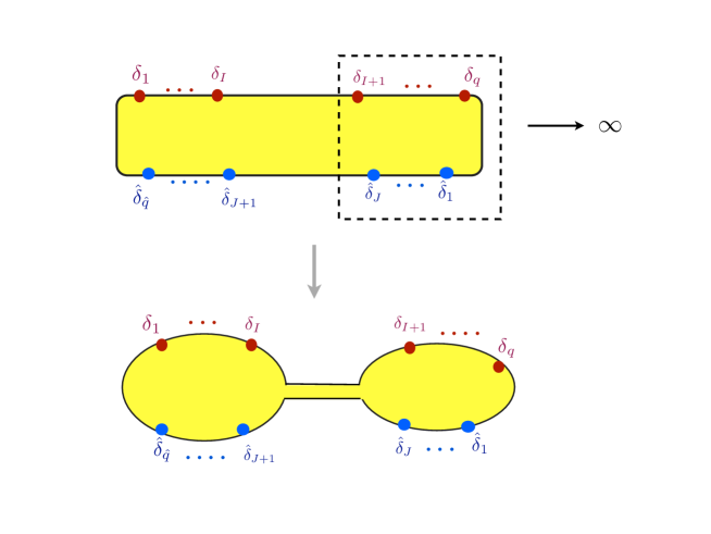
Figure 6: Schematic drawing of the factorization limit of five-brane singularities discussed in the text. The picture is meant to show the actual size of the strip geometry. The background consists of two, $AdS_{4}\ltimes K$ and $AdS_{4}\ltimes K^{\prime}$, solutions coupled through a narrow $AdS_{5}\times S^{5}$ bridge. The curvature of the narrow bridge is larger than the curvature in the rest of the geometry, but can be small enough so as to ignore quantum gravity corrections. The configuration resembles therefore a wormhole.

We can check that the partitions corresponding to these two solutions are exactly the ones obtained by the splitting of $(\rho,\hat{\rho})$ into two subpartitions by the saturation of the condition (2.5) for $r=\sum_{b=1}^{J}\hat{N}_{b}$. These partitions are explicitly :

$$\rho_{L} = \Big{(}\underbrace{l_{1}-\sum_{b=1}^{J}\hat{N}_{b},...,l_{1}-\sum_{b=1}^{J}\hat{N}_{b}}_{N_{1}},...,\underbrace{l_{I}-\sum_{b=1}^{J}\hat{N}_{b},...,l_{I}-\sum_{b=1}^{J}\hat{N}_{b}}_{N_{I}}\Big{)}$$

$$\hat{\rho}_{L} = \Big{(}\underbrace{\hat{l}_{J+1},...,\hat{l}_{J+1}}_{\hat{N}_{J+1}},...,\underbrace{\hat{l}_{\hat{q}},...,\hat{l}_{\hat{q}}}_{\hat{N}_{\hat{q}}}\Big{)}$$ (5.22)

and

$$\rho_{R} = \Big{(}\underbrace{l_{I+1},...,l_{I+1}}_{N_{I+1}},...,\underbrace{l_{q},...,l_{q}}_{N_{q}}\Big{)}$$

$$\hat{\rho}_{R} = \Big{(}\underbrace{\hat{l}_{1}-\sum_{a=1}^{I}N_{a},...,\hat{l}_{1}-\sum_{a=1}^{I}N_{a}}_{\hat{N}_{1}},...,\underbrace{\hat{l}_{J}-\sum_{a=1}^{I}N_{a},...,\hat{l}_{J}-\sum_{a=1}^{I}N_{a}}_{\hat{N}_{J}}\Big{)}$$ (5.23)

where the indices L, R refer to the left and right parts of the split quiver. The linking numbers have been here gauge transformed so as to make them agree, for each sub-quiver separately, with our earlier conventions. So the splitting of the quiver corresponds precisely to the factorization of the bulk geometry, confirming once again the holographic duality map.

As we have seen in section 3, the limit of capping off asymptotic $AdS_{5}\times S^{5}$ regions is smooth. We hope to return to the physics of this limit elsewhere.

6 Discussion

In this paper we have constructed the type-IIB supergravity solutions which are holographically dual to a rich family of three dimensional ${\mathcal{N}}=4$ superconformal field theories. These theories arise as infrared fixed points of the $T^{\rho}_{\hat{\rho}}(SU(N))$ and $T_{\rho}^{\hat{\rho}}(SU(N))$ quiver gauge theories whenever $\hat{\rho}^{T}>\rho$. This non-trivial constraint, together with the $H_{\rho}\times H_{\hat{\rho}}$ global symmetries of the associated superconformal field theory, have been precisely realized in our supergravity solutions.

Our explicit type-IIB supergravity solutions provide a novel arena in which to study this rich family of superconformal field theories. Even though the dilaton or curvature gets large near the location of five-brane singularities, our solution can be nicely interpreted in string theory by replacing the five-brane singularities by explicit five-branes, which give rise to important new light degrees of freedom localized in the geometry. Information regarding the spectrum of local and non-local operators in these conformal field theories can be obtained by studying the supergravity fluctuation spectrum around our $AdS_{4}\ltimes K$ solutions as well as by considering strings and branes ending on the boundary of our $AdS_{4}\ltimes K$ backgrounds along submanifolds of varying dimensionality.

Another very interesting direction is to use our supergravity solutions to determine the partition function $Z_{S^{3}}$ of the boundary field theory on $S^{3}$, obtained by evaluating the type-IIB string action on the $AdS_{4}\ltimes K$ solutions. Recently, it has been noted that the associated renormalized “free energy” [22, 23] (see also [24])

$$F=-\log|Z_{S^{3}}|$$ (6.24)

enjoys interesting monotonicity properties under renormalization group evolution. The partition function $Z_{S^{3}}$ of the infrared superconformal field theory associated to $T^{\rho}_{\hat{\rho}}(SU(N))$ deformed by FI and mass parameters has recently been calculated [3] (see also [25]) using the localization formulae in [26], and shown to reproduce the partition function of the mirror $T_{\rho}^{\hat{\rho}}(SU(N))$ theory upon exchanging the role of FI and mass parameters. By suitably taking the deformation parameters to their “superconformal” value, the formula for the partition function at the superconformal fixed point can be obtained, and compared with the one calculated from our supergravity solutions.

Also, as we have seen in this paper, the above type-IIB geometries have interesting factorization limits, as well as limits in which asymptotic $AdS_{5}\times S^{5}$ regions become very highly curved. The former can be thought of as wormhole-like solutions which describe two different $AdS_{4}\ltimes K$ regions, connected by an $AdS_{5}\times S^{5}$ throat, while in the latter limit a large $AdS_{4}\ltimes K$ region is extended to infinity along one or more very thin $AdS_{5}\times S^{5}$ fixtures or throats. We plan to return to the physics of these solutions, and whether they give a consistent string theory realization of massive gravity or multi-gravity.

Finally, we would like to point out that the solutions of type-IIB string theory constructed in this paper have no moduli! That is, the quantization condition of the various fluxes, and the presence of both NS5 and D5-branes in the geometry, fix all moduli, including the dilaton. It is interesting that rather simple and explicit isolated vacua of string theory can be explicitly constructed. It would be desirable to determine whether flux quantization in the presence of both NS5 and D5-branes can be used to construct phenomenologically more realistic vacua of string theory.

Aknowledgements: We thank D. Gaiotto and Y. Tachikawa for discussions. C.B. thanks the Alexander von Humboldt foundation and the Ludwig Maximilian Universität in Münich for hospitality in the final stages of this work. J.E. is supported by the FWO - Vlaanderen, Project No. G.0235.05, and by the “Federal Office for Scientific, Technical and Cultural Affairs through the Inter-University Attraction Poles Programme,” Belgian Science Policy P6/11-P. J.G. thanks the LPTENS, the LPTHE in Jussieu and the FRIF (“Federation de Recherche sur les Interactions Fondamentales”) for their hospitality during this work. J.G. further thanks the University of Barcelona for hospitality during the completion of this work. Research at the Perimeter Institute is supported in part by the Government of Canada through NSERC and by the Province of Ontario through MRI. J.G. also acknowledges further support from an NSERC Discovery Grant and from an ERA grant by the Province of Ontario.

References

- [1] J. M. Maldacena, “The Large N limit of superconformal field theories and supergravity,” Adv. Theor. Math. Phys. 2 (1998) 231-252. [hep-th/9711200].
- [2] D. Gaiotto, E. Witten, “S-Duality of Boundary Conditions In N=4 Super Yang-Mills Theory,” [arXiv:0807.3720 [hep-th]].
- [3] T. Nishioka, Y. Tachikawa and M. Yamazaki, “3d Partition Function as Overlap of Wavefunctions,” arXiv:1105.4390 [hep-th].
- [4] E. D’Hoker, J. Estes and M. Gutperle, “Exact half-BPS Type IIB interface solutions I: Local solution and supersymmetric Janus,” JHEP 0706 (2007) 021 [arXiv:0705.0022 [hep-th]].
- [5] E. D’Hoker, J. Estes and M. Gutperle, “Exact half-BPS type IIB interface solutions. II: Flux solutions and multi-janus,” JHEP 0706 (2007) 022 [arXiv:0705.0024 [hep-th]].
- [6] J. Gomis and C. Romelsberger, “Bubbling defect CFT’s,” JHEP 0608 (2006) 050 [arXiv:hep-th/0604155].
- [7] O. Lunin, “On gravitational description of Wilson lines,” JHEP 0606, 026 (2006). [hep-th/0604133].
- [8] D. Gaiotto, E. Witten, “Supersymmetric Boundary Conditions in N=4 Super Yang-Mills Theory,” [arXiv:0804.2902 [hep-th]].
- [9] C. Bachas, J. Estes, “Spin-2 spectrum of defect theories,” JHEP 1106 (2011) 005. [arXiv:1103.2800 [hep-th]].
- [10] O. Aharony, O. DeWolfe, D. Z. Freedman, A. Karch, “Defect conformal field theory and locally localized gravity,” JHEP 0307, 030 (2003). [hep-th/0303249].
- [11] E. Kiritsis, “Product CFTs, gravitational cloning, massive gravitons and the space of gravitational duals,” JHEP 0611 (2006) 049 [arXiv:hep-th/0608088].
- [12] O. Aharony, A. B. Clark and A. Karch, “The CFT/AdS correspondence, massive gravitons and a connectivity index conjecture,” Phys. Rev. D 74 (2006) 086006 [arXiv:hep-th/0608089].
- [13] O. Aharony, L. Berdichevsky, M. Berkooz, I. Shamir, “Near-horizon solutions for D3-branes ending on 5-branes,” [arXiv:1106.1870 [hep-th]].
- [14] K. A. Intriligator, N. Seiberg, “Mirror symmetry in three-dimensional gauge theories,” Phys. Lett. B387, 513-519 (1996). [hep-th/9607207].
- [15] A. Hanany, E. Witten, “Type IIB superstrings, BPS monopoles, and three-dimensional gauge dynamics,” Nucl. Phys. B492, 152-190 (1997). [hep-th/9611230].
- [16] C. P. Bachas, M. R. Douglas, M. B. Green, “Anomalous creation of branes,” JHEP 9707, 002 (1997). [hep-th/9705074].
- [17] C. P. Bachas, M. B. Green and A. Schwimmer, “(8,0) quantum mechanics and symmetry enhancement in type I’ superstrings,” JHEP 9801 (1998) 006 [arXiv:hep-th/9712086].
- [18] D. Marolf, “Chern-Simons terms and the three notions of charge,” [hep-th/0006117].
- [19] C. Bachas, M. R. Douglas, C. Schweigert, “Flux stabilization of D-branes,” JHEP 0005, 048 (2000). [hep-th/0003037].
- [20] M. S. Bianchi, S. Penati and M. Siani, “Infrared stability of ABJ-like theories,” JHEP 1001 (2010) 080 [arXiv:0910.5200 [hep-th]].
- [21] M. S. Bianchi, S. Penati and M. Siani, “Infrared Stability of N = 2 Chern-Simons Matter Theories,” JHEP 1005 (2010) 106 [arXiv:0912.4282 [hep-th]].
- [22] H. Casini, M. Huerta, R. C. Myers, “Towards a derivation of holographic entanglement entropy,” JHEP 1105, 036 (2011). [arXiv:1102.0440 [hep-th]].
- [23] D. L. Jafferis, I. R. Klebanov, S. S. Pufu, B. R. Safdi, “Towards the F-Theorem: N=2 Field Theories on the Three-Sphere,” [arXiv:1103.1181 [hep-th]].
- [24] A. Amariti and M. Siani, “Z-extremization and F-theorem in Chern-Simons matter theories,” arXiv:1105.0933 [hep-th].
- [25] S. Benvenuti and S. Pasquetti, “3D-partition functions on the sphere: exact evaluation and mirror symmetry,” arXiv:1105.2551 [hep-th].
- [26] A. Kapustin, B. Willett, I. Yaakov, “Exact Results for Wilson Loops in Superconformal Chern-Simons Theories with Matter,” JHEP 1003, 089 (2010). [arXiv:0909.4559 [hep-th]].
- [27] N. Drukker, M. Marino, P. Putrov, “From weak to strong coupling in ABJM theory,” [arXiv:1007.3837 [hep-th]].
- [28] D. Martelli, J. Sparks, “The large N limit of quiver matrix models and Sasaki-Einstein manifolds,” [arXiv:1102.5289 [hep-th]].
- [29] S. Cheon, H. Kim, N. Kim, “Calculating the partition function of N=2 Gauge theories on and AdS/CFT correspondence,” JHEP 1105, 134 (2011). [arXiv:1102.5565 [hep-th]].
- [30] D. R. Gulotta, C. P. Herzog, S. S. Pufu, “From Necklace Quivers to the F-theorem, Operator Counting, and T(U(N)),” [arXiv:1105.2817 [hep-th]].