Learning with the Weighted Trace-norm under Arbitrary Sampling Distributions

Abstract

We provide rigorous guarantees on learning with the weighted trace-norm under arbitrary sampling distributions. We show that the standard weighted trace-norm might fail when the sampling distribution is not a product distribution (i.e. when row and column indexes are not selected independently), present a corrected variant for which we establish strong learning guarantees, and demonstrate that it works better in practice. We provide guarantees when weighting by either the true or empirical sampling distribution, and suggest that even if the true distribution is known (or is uniform), weighting by the empirical distribution may be beneficial.

1 Introduction

One of the most common approaches to collaborative filtering and matrix completion is trace-norm regularization [1, 2, 3, 4]. In this approach we attempt to complete an unknown matrix, based on a small subset of revealed entries, by finding a matrix with small trace-norm, which matches those entries as best as possible.

This approach has repeatedly shown good performance in practice, and is theoretically well understood for the case where revealed entries are sampled uniformly [5, 6, 7, 8, 9, 10]. Under such uniform sampling, $\Theta(n\log(n))$ entries are sufficient for good completion of an $n\times n$ matrix—i.e. a nearly constant number of entries per row. However, for arbitrary sampling distributions, the worst-case sample complexity lies between a lower bound of $\mathbf{\Omega}(n^{4/3})$ [11] and an upper bound of $\mathbf{O}(n^{3/2})$ [12], i.e. requiring between $n^{1/3}$ and $n^{\nicefrac{{1}}{{2}}}$ observations per row, and indicating it is not appropriate for matrix completion in this setting.

Motivated by these issues, Salakhutdinov and Srebro [11] proposed to use a weighted variant of the trace-norm, which takes the distribution of the entries into account, and showed experimentally that this variant indeed leads to superior performance. However, although this recent paper established that the weighted trace-norm corrects a specific situation where the standard trace-norm fails, no general learning guarantees are provided, and it is not clear if indeed the weighted trace-norm always leads to the desired behavior. The only theoretical analysis of the weighted trace-norm that we are aware of is a recent report by Negahban and Wainwright [9] that provides reconstruction guarantees for a low-rank matrix with i.i.d. noise, but only when the sampling distribution is a product distribution, i.e. the rows index and column index of observed entries are selected independently. A product distribution assumption does not seem realistic in many cases—e.g. for the Netflix data, it would indicate that all users have the same (conditional) distribution over which movies they rate.

In this paper we rigorously study learning with a weighted trace-norm under an arbitrary sampling distribution, and show that this situation is indeed more complicated, requiring a correction to the weighting. We show that this correction is necessary, and present empirical results on the Netflix and MovieLens dataset indicating that it is also helpful in practice. We also rigorously consider weighting according to either the true sampling distribution (as in [9]) or the empirical frequencies, as is actually done in practice, and present evidence that weighting by the empirical frequencies might be advantageous. Our setting is also more general then that of [9]—we consider an arbitrary loss and do not rely in i.i.d. noise, instead presenting results in an agnostic learning framework.

Setup and Notation.

We consider an arbitrary unknown $n\times m$ target matrix $Y$, where a subset of entries $\{Y_{i_{t},j_{t}}\}_{t=1}^{s}$ indexed by $S=\left\{(i_{1},j_{1}),\dots,(i_{s},j_{s})\right\}$ is revealed to us. Without loss of generality, we assume $n\geq m$. Throughout most of the paper, we assume $S$ is drawn i.i.d. according to some sampling distribution $p(i,j)$ (with replacement). Based on this subset on entries, we would like to fill in the missing entries and obtain a prediction matrix $\hat{X}_{S}\in\mathbb{R}^{n\times m}$, with low expected loss $L_{p}(\hat{X}_{S})={{\mbox{\bf E}}_{ij\sim p}\left[{\ell((\hat{X}_{S})_{ij},Y_{ij})}\right]}$, where $\ell(x,y)$ is some loss function. Note that we measure the loss with respect to the same distribution $p(i,j)$ from which the training set is drawn (this is also the case in [11, 9, 12]).

Given some distribution $p(i,j)$ on $[n]\times[m]$, the weighted trace-norm of a matrix $X\in\mathbb{R}^{n\times m}$ is given by [11]

$$\left\|{X}\right\|_{\mathrm{tr}\left(p^{r},p^{c}\right)}=\left\|{\mathrm{diag}\left({p^{r}}\right)^{\nicefrac{{1}}{{2}}}\cdot X\cdot\mathrm{diag}\left({p^{c}}\right)^{\nicefrac{{1}}{{2}}}}\right\|_{\mathrm{tr}}\;,$$

where $p^{r}\in\mathbb{R}^{n}$ and $p^{c}\in\mathbb{R}^{m}$ denote vectors of the row- and column-marginals respectively. Note that the weighted trace-norm only depends on these marginals (but not their joint distribution) and that if $p^{r}$ and $p^{c}$ are uniform, then $\left\|{X}\right\|_{\mathrm{tr}\left(p^{r},p^{c}\right)}=\frac{1}{\sqrt{nm}}\left\|{X}\right\|_{\mathrm{tr}}$. The weighted trace-norm does not generally scale with $n$ and $m$, and in particular, if $X$ has rank $r$ and entries bounded in $[-1,1]$, then $\left\|{X}\right\|_{\mathrm{tr}\left(p^{r},p^{c}\right)}\leq\sqrt{r}$ regardless of which $p\left({i},{j}\right)$ is used. This motivates us to define the class

$$\mathcal{W}_{r}\left[{p}\right]=\{X\in\mathbb{R}^{n\times m}:\left\|{X}\right\|_{\mathrm{tr}\left(p^{r},p^{c}\right)}\leq\sqrt{r}\},$$

although we emphasize that our results do not directly depend on the rank, and $\mathcal{W}_{r}\left[{p}\right]$ certainly includes full-rank matrices. We analyze here estimators of the form $\hat{X}_{S}=\arg\min\{\hat{L}_{S}(X)\ :\ X\in\mathcal{W}_{r}\left[{p}\right]\}$ where $\hat{L}_{S}(X)=\frac{1}{s}\sum_{t=1}^{s}\ell(X_{i_{t},j_{t}},Y_{i_{t},j_{t}})$ is the empirical error on the observed entries.

Although we focus mostly on the standard inductive setting, where the samples are drawn i.i.d. and the guarantee is on generalization for future samples drawn by the same distribution, our results can also be stated in a transductive model, where a training set and a test set are created by splitting a fixed subset of entries uniformly at random (as in [12]). The transductive setting is discussed in Section 4.2, and variants of our Theorems in this setting are found there and in Appendix B.

2 Learning with the Standard Weighting

In this Section, we consider learning using the weighted trace-norm as suggested by Salakhutdinov and Srebro [11], i.e. when the weighting is according to the sampling distribution $p(i,j)$. Following the approach of [5] and [10], we base our results on bounding the Rademacher complexity of $\mathcal{W}_{r}\left[{p}\right]$, as a class of functions mapping index pairs to entry values. However, we modify the analysis for the weighted trace-norm with non-uniform sampling.

For a class of matrices $\mathcal{X}$ and a sample $S=\left\{(i_{1},j_{1}),\dots,(i_{s},j_{s})\right\}$ of indexes in $[n]\times[m]$, the empirical Rademacher complexity of the class (with respect to $S$) is given by

$$\hat{\mathcal{R}}_{S}(\mathcal{X})={{\mbox{\bf E}}_{\sigma\sim\{\pm 1\}^{s}}\left[{\sup_{X\in\mathcal{X}}\frac{1}{s}\sum_{t=1}^{s}\sigma_{t}X_{i_{t}j_{t}}}\right]}\;,$$

where $\sigma$ is a vector of signs drawn uniformly at random. Intuitively, $\hat{\mathcal{R}}_{S}(\mathcal{X})$ measures the extent to which the class $\mathcal{X}$ can “overfit” data, by finding a matrix $X$ which correlates as strongly as possible to a sample from a matrix of random noise. For a loss $\ell(x,y)$ that is Lipschitz in $x$, the Rademacher complexity can be used to uniformly bound the deviations $|L_{p}(X)-\hat{L}_{S}(X)|$ for all $X\in\mathcal{X}$, yielding a learning guarantee on the empirical risk minimizer [13].

2.1 Guarantees for Special Sampling Distributions

We begin by providing guarantees for an arbitrary, possibly unbounded, Lipschitz loss $\ell(x,y)$, but only under sampling distributions which are either product distributions (i.e. $p(i,j)=p^{r}(i)p^{c}(j)$) or have uniform marginals (i.e. $p^{r}$ and $p^{c}$ are uniform, but perhaps the rows and columns are not independent). In Section 2.3 below, we will see why this severe restriction on $p$ is needed.

Theorem 1.

For an $l$-Lipschitz loss $\ell$, fix any matrix $Y$, sample size $s$, and distribution $p$, such that $p$ is either a product distribution or has uniform marginals.

Let $\hat{X}_{S}=\arg\min\left\{\hat{L}_{S}(X)\ :\ X\in\mathcal{W}_{r}\left[{p}\right]\right\}$. Then, in expectation over the training sample $S$ drawn i.i.d. from the distribution $p$,

$$L_{p}(\hat{X}_{S})\leq\inf_{X\in\mathcal{W}_{r}\left[{p}\right]}L_{p}(X)+\mathbf{O}\left(l\cdot\sqrt{\frac{rn\log(n)}{s}}\right)\;.$$ (1)

Here and elsewhere we state learning guarantees in expectation for simplicity, but all guarantees can also be obtained with high probability.

Proof.

We will show how to bound the expected Rademacher complexity ${{\mbox{\bf E}}_{S}\left[{\hat{\mathcal{R}}_{S}(\mathcal{W}_{r}\left[{p}\right])}\right]}$, from which the desired results follows using standard arguments [13].

Following [10] by including the weights, using the duality between spectral norm $\left\lVert{\cdot}\right\rVert_{\mathrm{sp}}$ and trace-norm, we compute:

$${{\mbox{\bf E}}_{S}\left[{\hat{\mathcal{R}}_{S}(\mathcal{W}_{r}\left[{p}\right])}\right]}=\frac{\sqrt{r}}{s}{{\mbox{\bf E}}_{S,\sigma}\left[{\left\lVert{\sum_{t=1}^{s}\sigma_{t}\frac{e_{i_{t},j_{t}}}{\sqrt{p^{r}\left({i_{t}}\right)p^{c}\left({j_{t}}\right)}}}\right\rVert_{\mathrm{sp}}}\right]}=\frac{\sqrt{r}}{s}{{\mbox{\bf E}}_{S,\sigma}\left[{\left\lVert{\sum_{t=1}^{s}Q_{t}}\right\rVert_{\mathrm{sp}}}\right]}\;,$$

where $e_{i,j}=e_{i}e_{j}^{T}$ and $Q_{t}=\sigma_{t}\frac{e_{i_{t},j_{t}}}{\sqrt{p^{r}\left({i_{t}}\right)p^{c}\left({j_{t}}\right)}}\in\mathbb{R}^{n\times m}$. Since the $Q_{t}$’s are i.i.d. zero-mean matrices, Theorem 6.1 of [14], combined with Remarks 6.4 and 6.5 there, establishes that

$${{\mbox{\bf E}}_{S,\sigma}\left[{\left\lVert{\sum_{t=1}^{s}Q_{t}}\right\rVert_{\mathrm{sp}}}\right]}=\mathbf{O}\left(\sigma\sqrt{\log(n)}+R\log(n)\right)\;,$$

where $\left\lVert{Q_{t}}\right\rVert_{\mathrm{sp}}\leq R$ (almost surely) and $\sigma^{2}=\max\left\{\left\lVert{\sum{{\mbox{\bf E}}\left[{Q_{t}^{T}Q_{t}}\right]}}\right\rVert_{\mathrm{sp}},\left\lVert{\sum{{\mbox{\bf E}}\left[{Q_{t}Q^{T}_{t}}\right]}}\right\rVert_{\mathrm{sp}}\right\}$. Calculating these (see Appendix A ), we get $R\leq\sqrt{\frac{nm}{\min_{i,j}\{np^{r}\left({i}\right)\cdot mp^{c}\left({j}\right)\}}}$, and

$$\sigma\leq\sqrt{s\max\left\{\max_{i}\sum_{j}\frac{p\left({i},{j}\right)}{p^{r}\left({i}\right)p^{c}\left({j}\right)},\max_{j}\sum_{i}\frac{p\left({i},{j}\right)}{p^{r}\left({i}\right)p^{c}\left({j}\right)}\right\}}\leq\sqrt{\frac{sn}{\min_{i,j}\{np^{r}\left({i}\right)\cdot mp^{c}\left({j}\right)\}}}\;.$$

If $p$ has uniform row- and column-marginals, then for all $i,j$, $np^{r}\left({i}\right)=mp^{c}\left({j}\right)=1$. This yields

$${{\mbox{\bf E}}_{S}\left[{\hat{\mathcal{R}}(\mathcal{W}_{r}\left[{p}\right])}\right]}\leq\mathbf{O}\left(\sqrt{\frac{rn\log(n)}{s}}\right)\;,$$

as desired. (Here we assume $s>n\log(n)$, since otherwise we need only establish that excess error is $O(l\sqrt{r})$, which holds trivially for any matrix in $\mathcal{W}_{r}\left[{p}\right]$.)

If $p$ does not have uniform marginals, but instead is a product distribution, then the quantity $R$ defined above is potentially unbounded, so we cannot apply the same simple argument. However, we can consider the “$p$-truncated” class of matrices

$$\mathcal{Z}=\left\{Z(X)=\left(X_{ij}\mathbb{I}\left\{{p\left({i},{j}\right)\geq\frac{\log(n)}{s\sqrt{nm}}}\right\}\right)_{ij}:X\in\mathcal{W}_{r}\left[{p}\right]\right\}\;.$$

By a similar calculation of the expected spectral norms, we can now bound ${{\mbox{\bf E}}_{S}\left[{\hat{\mathcal{R}}_{S}(\mathcal{Z})}\right]}\leq\mathbf{O}\left(\sqrt{\frac{rn\log(n)}{s}}\right)$. Applying [13], this bounds $\left(L_{p}(Z(\hat{X}_{S}))-\hat{L}_{S}(Z(\hat{X}_{S}))\right)$ (in expectation). Since $Z(\hat{X}_{S})_{ij}\neq(\hat{X}_{S})_{ij}$ only on the extremely low-probability entries, we can also bound $\left(L_{p}(\hat{X}_{S})-L_{p}(Z(\hat{X}_{S}))\right)$ and $\left(\hat{L}_{S}(Z(\hat{X}_{S}))-\hat{L}_{S}(\hat{X}_{S})\right)$. Combining these steps, we can bound $\left(L_{p}(\hat{X}_{S})-\hat{L}_{S}(\hat{X}_{S})\right)$. We similarly bound $\hat{L}_{S}(X^{*})-L_{p}(X^{*})$, where $X^{*}=\arg\min_{X\in\mathcal{W}_{r}\left[{p}\right]}L_{p}(X)$. Since $\hat{L}_{S}(\hat{X}_{S})\leq\hat{L}_{S}(X^{*})$, this yields the desired bound on excess error. The details are given in Appendix A. ∎

Examining the proof of Theorem 1, we see that we can generalize the result by including distributions $p$ with row- and column-marginals that are lower-bounded. More precisely, if $p$ satisfies $p^{r}\left({i}\right)\geq\frac{1}{Cn}$, $p^{c}\left({j}\right)\geq\frac{1}{Cm}$ for all $i,j$, then the bound (1) holds, up to a factor of $C$. Note that this result does not require an upper bound on the row- and column-marginals, only a lower bound, i.e. it only requires that no marginals are too low. This is important to note since the examples where the unweighted trace-norm fails under a non-uniform distribution are situations where some marginals are very high (but none are too low)  [11]. This suggests that the low-probability marginals could perhaps be “smoothed” to satisfy a lower bound, without removing the advantages of the weighted trace-norm. We will exploit this in Section 3 to give a guarantee that holds more generally for arbitrary $p$, when smoothing is applied.

2.2 Guarantees for bounded loss

In Theorem 1, we showed a strong bound on excess error, but only for a restricted class of distributions $p$. We now show that if the loss function $\ell$ is bounded, then we can give a non-trivial, but weaker, learning guarantee that holds uniformly over all distributions $p$. Since we are in any case discussing Lipschitz loss functions, requiring that the loss function be bounded essentially amounts to requiring that the entries of the matrices involved be bounded. That is, we can view this as a guarantee on learning matrices with bounded entries. In Section 2.3 below, we will show that this boundedness assumption is unavoidable if we want to give a guarantee that holds for arbitrary $p$.

Theorem 2.

For an $l$-Lipschitz loss $\ell$ bounded by $b$, fix any matrix $Y$, sample size $s$, and any distribution $p$. Let $\hat{X}_{S}=\arg\min\left\{\hat{L}_{S}(X)\ :\ X\in\mathcal{W}_{r}\left[{p}\right]\right\}$ for $r\geq 1$. Then, in expectation over the training sample $S$ drawn i.i.d. from the distribution $p$,

$$L_{p}(\hat{X}_{S})\leq\inf_{X\in\mathcal{W}_{r}\left[{p}\right]}L_{p}(X)+\mathbf{O}\left((l+b)\cdot\sqrt[3]{\frac{rn\log(n)}{s}}\right)\;.$$ (2)

The proof is provided in Appendix A, and is again based on analyzing the expected Rademacher complexity, ${{\mbox{\bf E}}_{S}\left[{\hat{\mathcal{R}}(\ell\circ\mathcal{W}_{r}\left[{p}\right])}\right]}\leq\mathbf{O}\left((l+b)\cdot\sqrt[3]{\frac{rn\log(n)}{s}}\right)$.

2.3 Problems with the standard weighting

In the previous Sections, we showed that for distributions $p$ that are either product distributions or have uniform marginals, we can prove a square-root bound on excess error, as shown in (1). For arbitrary $p$, the only learning guarantee we obtain is a cube-root bound given in (2), for the special case of bounded loss. We would like to know whether the square-root bound might hold uniformly over all distributions $p$, and if not, whether the cube-root bound is the strongest result that we can give in this case for the bounded-loss setting, and whether any bound will hold uniformly over all $p$ in the unbounded-loss setting.

The examples below demonstrate that we cannot improve the results of Theorems 1 and 2 (up to log factors), by constructing degenerate examples using non-product distributions $p$ with non-uniform marginals. Specifically, in Example 1, we show that in the special case of bounded loss, the cube-root bound in 2 is the best possible bound (up to the log factor) that will hold for all $p$, by giving a construction for arbitrary $n=m$ and arbitrary $s\leq nm$, such that with $1$-bounded loss, excess error is ${\mathbf{\Omega}}\left(\sqrt[3]{\frac{n}{s}}\right)$. In Example 2, we show that with unbounded (Lipschitz) loss, we cannot bound excess error better than a constant bound, by giving a construction for arbitrary $n=m$ and arbitrary $s\leq nm$ in the unbounded-loss regime, where excess error is $\mathbf{\Omega}(1)$. For both examples we fix $r=1$. We note that both examples can be modified to fit the transductive setting, demonstrating that smoothing is necessary also in the transductive setting as well.

Example 1. Let $\ell(x,y)=\min\{1,|x-y|\}\leq 1$, let $a=(2s/n)^{\nicefrac{{2}}{{3}}}<n$, and let matrix $Y$ and block-wise constant distribution $p$ be given by

$$Y=\left(\begin{array}[]{cc}A&\mathbf{0}_{a\times\tfrac{n}{2}}\\ \mathbf{0}_{(n-a)\times\tfrac{n}{2}}&\mathbf{0}_{(n-a)\times\tfrac{n}{2}}\\ \end{array}\right)\;,\ \ (p\left({i},{j}\right))=\left(\begin{array}[]{cc}\frac{1}{2s}\cdot\mathbf{1}_{a\times\tfrac{n}{2}}&\mathbf{0}_{a\times\tfrac{n}{2}}\\ \mathbf{0}_{(n-a)\times\tfrac{n}{2}}&\frac{1-\tfrac{an}{4s}}{(n-a)\frac{n}{2}}\cdot\mathbf{1}_{(n-a)\times\tfrac{n}{2}}\\ \end{array}\right)\;,$$

where $A\in\{\pm 1\}^{a\times\tfrac{n}{2}}$ is any sign matrix. Clearly, $\left\|{Y}\right\|_{\mathrm{tr}\left(p^{r},p^{c}\right)}\leq 1$, and so $\inf_{X\in\mathcal{W}_{r}\left[{p}\right]}L_{p}(X)=0$. Now suppose we draw a sample $S$ of size $s$ from the matrix $Y$, according to the distribution $p$. We will show an ERM $\hat{Y}$ such that in expectation over $S$, $L_{p}(\hat{Y})\geq\frac{1}{8}\sqrt[3]{\frac{n}{s}}$.

Consider $Y^{S}$ where $Y^{S}_{ij}=Y_{ij}\mathbb{I}\left\{{ij\in S}\right\}$, and note that $\left\|{Y^{S}}\right\|_{\mathrm{tr}\left(p^{r},p^{c}\right)}\leq 1$. Since $\hat{L}_{S}(Y^{S})=0$, it clearly an ERM. We also have $L_{p}(Y^{S})=\frac{N}{2s}$, where $N$ is the number of $\pm 1$’s in $Y$ which are not observed in the sample. Since ${{\mbox{\bf E}}\left[{N}\right]}\geq\frac{an}{4}$, we see that ${{\mbox{\bf E}}\left[{L_{p}(Y^{S})}\right]}\geq\frac{1}{2s}\cdot\frac{an}{4}\geq\frac{1}{8}\sqrt[3]{\frac{n}{s}}$.

Example 2. Let $\ell(x,y)=|x-y|$. Let $Y=\mathbf{0}_{n\times n}$; trivially, $Y\in\mathcal{W}_{r}\left[{p}\right]$. Let $p\left({1},{1}\right)=\frac{1}{s}$, and $p\left({i},{1}\right)=p\left({1},{j}\right)=0$ for all $i,j>1$, yielding $p^{r}\left({1}\right)=p^{c}\left({1}\right)=\frac{1}{s}$. (The other entries of $p$ may be defined arbitrarily.) We will show an ERM $\hat{Y}$ such that, in expectation over $S$, $L_{p}(\hat{Y})\geq 0.25$. Let $A$ be the matrix with $X_{11}=s$ and zeros elsewhere, and note that $\left\|{A}\right\|_{\mathrm{tr}\left(p^{r},p^{c}\right)}=1$. With probability $\geq 0.25$, entry $(1,1)$ will not appear in $S$, in which case $\hat{Y}=A$ is an ERM, with $L_{p}(\hat{Y})=1$.

The following table summarizes the learning guarantees that can be established for the (standard) weighted trace-norm. As we saw, these guarantees are tight up to log-factors.

	$1$-Lipschitz, $1$-bounded loss	$1$-Lipschitz, unbounded loss
$p=$ product	$\sqrt{\frac{rn\log(n)}{s}}$	$\sqrt{\frac{rn\log(n)}{s}}$
$p^{r},p^{c}=$ uniform	$\sqrt{\frac{rn\log(n)}{s}}$	$\sqrt{\frac{rn\log(n)}{s}}$
$p$ arbitrary	$\sqrt[3]{\frac{rn\log(n)}{s}}$	1

3 Smoothing the weighted trace norm

Considering Theorem 1 and the degenerate examples in Section 2.3, it seems that in order to be able to generalize for non-product distributions, we need to enforce some sort of uniformity on the weights. The Rademacher complexity computations in the proof of Theorem 1 show that the problem lies not with large entries in the vectors $p^{r}$ and $p^{c}$ (i.e. if $p^{r}$ and/or $p^{c}$ are “spiky”), but with the small entries in these vectors. This suggests the possibility of “smoothing” any overly low row- or column-marginals, in order to improve learning guarantees.

In Section 3.1, we present such a smoothing, and provide guarantees for learning with a smoothed weighted trace-norm. The result suggests that there is no strong negative consequence to smoothing, but there might be a large advantage, if confronted with situations as in Examples 1 and 2. In Section 3.2 we check the smoothing correction to the weighted trace-norm on real data, and observe that indeed it can also be beneficial in practice.

3.1 Learning guarantee for arbitrary distributions

Fix a distribution $p$ and a constant $\alpha\in(0,1)$, and let $\tilde{p}$ denote the smoothed marginals:

$$\tilde{p}^{r}\left({i}\right)=\alpha\cdot p^{r}\left({i}\right)+(1-\alpha)\cdot\tfrac{1}{n},\ \ \ \tilde{p}^{c}\left({j}\right)=\alpha\cdot p^{c}\left({j}\right)+(1-\alpha)\cdot\tfrac{1}{m}\;.$$ (3)

In the theoretical results below, we use $\alpha=\frac{1}{2}$, but up to a constant factor, the same results hold for any fixed choice of $\alpha\in(0,1)$.

Theorem 3.

For an $l$-Lipschitz loss $\ell$, fix any matrix $Y$, sample size $s$, and any distribution $p$. Let $\hat{X}_{S}=\arg\min\left\{\hat{L}_{S}(X)\ :\ X\in\mathcal{W}_{r}\left[{\tilde{p}}\right]\right\}$. Then, in expectation over the training sample $S$ drawn i.i.d. from the distribution $p$,

$$L_{p}(\hat{X}_{S})\leq\inf_{X\in\mathcal{W}_{r}\left[{\tilde{p}}\right]}L_{p}(X)+\mathbf{O}\left(l\cdot\sqrt{\frac{rn\log(n)}{s}}\right)\;.$$ (4)

Proof.

We bound ${{\mbox{\bf E}}_{S\sim p}\left[{\hat{\mathcal{R}}_{S}(\mathcal{W}_{r}\left[{\tilde{p}}\right])}\right]}\leq\mathbf{O}\left(\sqrt{\frac{rn\log(n)}{s}}\right)$, and then apply [13]. The proof of this Rademacher bound is essentially identical to the proof in Theorem 1, with the modified definition of $Q_{t}=\sigma_{t}\frac{e_{i_{t},j_{t}}}{\sqrt{\tilde{p}^{r}\left({i}\right)\tilde{p}^{c}\left({j}\right)}}$. Then $\left\lVert{Q_{t}}\right\rVert_{\mathrm{sp}}\leq\max_{ij}\frac{1}{\sqrt{\tilde{p}^{r}\left({i}\right)\tilde{p}^{c}\left({j}\right)}}\leq 2\sqrt{nm}\doteq R$, and ${{\mbox{\bf E}}\left[{\left\lVert{\sum_{t=1}^{s}Q_{t}Q_{t}^{T}}\right\rVert_{\mathrm{sp}}}\right]}=s\cdot{\max_{i}\sum_{j}\frac{p\left({i},{j}\right)}{\tilde{p}^{r}\left({i}\right)\tilde{p}^{c}\left({j}\right)}}\leq s\cdot{\max_{i}\sum_{j}\frac{p\left({i},{j}\right)}{\frac{1}{2}p^{r}\left({i}\right)\cdot\frac{1}{2m}}}\leq{4sm}$.

Similarly, ${{\mbox{\bf E}}\left[{\left\lVert{\sum_{t=1}^{s}Q_{t}^{T}Q_{t}}\right\rVert_{\mathrm{sp}}}\right]}\leq{4sn}$. Setting $\sigma\doteq\sqrt{4sn}$ and applying [14], we obtain the result. ∎

Moving from Theorem 1 to Theorem 3, we are competing with a different class of matrices:

$$\inf_{X\in\mathcal{W}_{r}\left[{p}\right]}L_{p}(X)\rightsquigarrow\inf_{X\in\mathcal{W}_{r}\left[{\tilde{p}}\right]}L_{p}(X)\;.$$

In most applications we can think of, this change is not significant. For example, we consider the low-rank matrix reconstruction problem, where the trace-norm bound is used as a surrogate for rank. In order for the (squared) weighted trace-norm to be a lower bound on the rank, we would need to assume $\left\|{\mathrm{diag}\left({p^{r}}\right)^{\nicefrac{{1}}{{2}}}X\mathrm{diag}\left({p^{c}}\right)^{\nicefrac{{1}}{{2}}}}\right\|_{F}^{2}\leq 1$ [10]. If we also assume that $\left\lVert{(X^{*})_{(i)}}\right\rVert^{2}_{2}\leq m$ and $\left\lVert{(X^{*})^{(j)}}\right\rVert^{2}_{2}\leq n$ for all rows $i$ and columns $j$ — i.e. the row and column magnitudes are not “spiky” — then $X^{*}\in\mathcal{W}_{r}\left[{\tilde{p}}\right]$. Note that this condition is much weaker than placing a spikiness condition on $X^{*}$ itself, e.g. requiring $\left|{X^{*}}\right|_{\infty}\leq 1$.

3.2 Results on Netflix and MovieLens Datasets

We evaluated different models on two publicly-available collaborative filtering datasets: Netflix [15] and MovieLens [16]. The Netflix dataset consists of 100,480,507 ratings from 480,189 users on 17,770 movies. Netflix also provides qualification set containing 1,408,395 ratings, but due to the sampling scheme, ratings from users with few ratings are overrepresented relative to the training set. To avoid dealing with different training and test distributions, we also created our own validation and test sets, each containing 100,000 ratings set aside from the training set. The MovieLens dataset contains 10,000,054 ratings from 71,567 users and 10,681 movies. We again set aside test and validation sets of 100,000 ratings. Ratings were normalized to be zero-mean.

When dealing with large datasets the most practical way to fit trace-norm regularized models is via stochastic gradient descent [17, 2, 11]. For computational reasons, however, we consider rank-truncated trace-norm minimization, by optimizing within the restricted class $\{X:X\in\mathcal{W}_{r}\left[{p}\right],\mathrm{rank}\left({X}\right)\leq k\}$ for $k=30$ and $k=100$, and for various values of smoothing parameters $\alpha$ (as in (3)). For each value of $\alpha$ and $k$, the regularization parameter was chosen by cross-validation.

The following table shows root mean squared error (RMSE) for the experiments. For both k=30 and k=100 the weighted trace-norm with smoothing significantly outperforms the weighted trace-norm without smoothing ($\alpha=1$), even on the differently-sampled Netflix qualification set. We also note that the proposed weighted trace-norm with smoothing outperforms max-norm regularization [18], and compares favorably with the “geometric” smoothing used by [11] as a heuristic, without theoretical or conceptual justification. A moderate value of $\alpha=0.9$ seems consistently good.

		Netflix					MovieLens
$\alpha$	k	Test	Qual	k	Test	Qual	k	Test	k	Test
1	30	0.7604	0.9107	100	0.7404	0.9078	30	0.7852	100	0.7821
0.9	30	0.7589	0.9096	100	0.7391	0.9068	30	0.7831	100	0.7798
0.5	30	0.7601	0.9173	100	0.7419	0.9161	30	0.7836	100	0.7815
0.3	30	0.7712	0.9198	100	0.7528	0.9207	30	0.7864	100	0.7871
0	30	0.7887	0.9249	100	0.7659	0.9236	30	0.7997	100	0.7987

4 The empirically-weighted trace norm

In practice, the sampling distribution $p$ is not known exactly — it can only be estimated via the locations of the entries which are observed in the sample. Defining the empirical marginals

$$\hat{p}^{r}\left({i}\right)=\frac{\#\{t:i_{t}=i\}}{s},\ \hat{p}^{c}\left({j}\right)=\frac{\#\{t:j_{t}=j\}}{s}\;,$$

we would like to give a learning guarantee when $\hat{X}_{S}$ is estimated via regularization on the $\hat{p}$-weighted trace-norm, rather than the $p$-weighted trace-norm.

In Section 4.1, we give bounds on excess error when learning with smoothed empirical marginals, which show that there is no theoretical disadvantage as compared to learning with the smoothed true marginals. In fact, we provide evidence that suggests there might even be an advantage to using the empirical marginals. To this end, in Section 4.2, we introduce the transductive learning setting, and give a result based on the empirical marginals which implies a sample complexity bound that is better by a factor of $\log^{\nicefrac{{1}}{{2}}}(n)$. In Section 4.3, we show that in low-rank matrix reconstruction simulations, using empirical marginals is indeed yields better reconstructions.

4.1 Guarantee for the standard (inductive) setting

We first show that when learning with the smoothed empirical marginals, defined as

$$\check{p}^{r}\left({i}\right)=\tfrac{1}{2}\left(\hat{p}^{r}\left({i}\right)+\tfrac{1}{n}\right),\ \check{p}^{c}\left({j}\right)=\tfrac{1}{2}\left(\hat{p}^{c}\left({j}\right)+\tfrac{1}{m}\right)\;,$$

we can obtain the same guarantee as for learning with the smoothed (true) marginals, given by $\tilde{p}$.

Theorem 4.

For an $l$-Lipschitz loss $\ell$, fix any matrix $Y$, sample size $s$, and any distribution $p$. Let $\hat{X}_{S}=\arg\min\left\{\hat{L}_{S}(X)\ :\ X\in\mathcal{W}_{r}\left[{\check{p}}\right]\right\}$. Then, in expectation over the training sample $S$ drawn i.i.d. from the distribution $p$,

$$L_{p}(\hat{X}_{S})\leq\inf_{X\in\mathcal{W}_{r}\left[{\tilde{p}}\right]}L_{p}(X)+\mathbf{O}\left(l\cdot\sqrt{\frac{r\max\{n,m\}\log(n+m)}{s}}\right)\;.$$ (5)

Note that although we regularize using the (smoothed) empirically-weighted trace-norm, we still compare ourselves to the best possible matrix in the class defined by the (smoothed) true marginals.

The proof of the Theorem (given in Appendix A) uses Theorem 3 and involves showing that with a sample of size $s=\mathbf{\Omega}(n\log(n))$, which is required for all Theorems so far to be meaningful, the true and empirical marginals are the same up to a constant factor. For this to be the case, such a sample size is even necessary. In fact, the $\log(n)$ factor in our analysis (e.g. in the proof of Theorem 1) arises from the bound on the expected spectral norm of a matrix, which, for a diagonal matrix, is just a bound on the deviation of empirical frequencies. Might it be possible, then, to avoid this logarithmic factor by using the empirical marginals? Although we could not establish such a result in the inductive setting, we now turn to the transductive setting, where we could indeed obtain a better guarantee.

4.2 Guarantee for the transductive setting

In the transductive model, we fix a set $\overline{S}\subset[n]\times[m]$ of size $2s$, and then randomly split $\overline{S}$ into a training set $S$ and a test set $T$ of equal size $s$. The goal is to obtain a good estimator for the entries in $T$ based on the values of the entries in $S$, as well as the locations (indexes) of all elements on $\overline{S}$. We then use the (smoothed or unsmoothed) empirical marginals of $\overline{S}$, for the weighted trace-norm.

We now show that, for bounded loss, there may be a benefit to weighting with the smoothed empirical marginals — the sample size requirement can be lowered to $s=\mathbf{O}\left(rn\log^{\nicefrac{{1}}{{2}}}(n)\right)$.

Theorem 5.

For an $l$-Lipschitz loss $\ell$ bounded by $b$, fix any matrix $Y$ and sample size $s$. Let $\overline{S}\subset[n]\times[m]$ be a fixed subset of size $2s$, split uniformly at random into training and test sets $S$ and $T$, each of size $s$. Let $\overline{p}$ denote the smoothed empirical marginals of $\overline{S}$. Let $\hat{X}_{S}=\arg\min\left\{\hat{L}_{S}(X)\ :\ X\in\mathcal{W}_{r}\left[{\overline{p}}\right]\right\}$. Then in expectation over the splitting of $\overline{S}$ into $S$ and $T$,

$$\hat{L}_{T}(\hat{X}_{S})\leq\inf_{X\in\mathcal{W}_{r}\left[{\overline{p}}\right]}\hat{L}_{T}(X)+\mathbf{O}\left(l\cdot\sqrt{\frac{rn\log^{\nicefrac{{1}}{{2}}}(n)}{s}}+\frac{b}{\sqrt{s}}\right)\;.$$ (6)

This result (proved in Appendix B) is stated in the transductive setting, with a somewhat different sampling procedure and evaluation criteria, but we believe the main difference is in the use of the empirical weights. Although it is usually straightforward to convert a transductive guarantee to an inductive one, the situation here is more complicated, since the hypothesis class depends on the weighting, and hence on the sample $\overline{S}$. Nevertheless, we believe such a conversion might be possible, establishing a similar guarantee for learning with the (smoothed) empirically weighted trace-norm also in the inductive setting. Furthermore, by using the fact that a sample of size $s=\Theta(n\log(n))$ is sufficient for the empirical marginals to be close to the true marginals, it might be possible to obtain a learning guarantee for the true (non-empirical) weighting with a sample of size $s=\mathbf{O}(n(r\log^{\nicefrac{{1}}{{2}}}(n)+\log(n)))$.

Theorem 5 above can be viewed as a transductive analog to Theorem 3 (where weights are based on the combined sample $\overline{S}$). In Appendix B we state and prove transductive analogs also to Theorem 1 (for the case where smoothing is not needed) and Theorem 2 (giving a cubic-root rate). As mentioned in Section 2.3, our lower bound examples can also be stated in the transductive setting, and thus all our guarantees and lower bounds can also be obtained in this setting.

4.3 Simulations with empirical weights

In order to numerically investigate the possible advantage of empirical weighting, we performed simulations on low-rank matrix reconstruction under uniform sampling with the unweighted, and the smoothed empirically weighted, trace-norms. We choose to work with uniform sampling in order to emphasize the benefit of empirical weights, even in situations where one might not consider to use any weights at all. In all the experiments, we attempt to reconstruct a possibly noisy, random rank-2 “signal” matrix $M$ with singular values $\tfrac{1}{\sqrt{2}}(n,n,0,\dots,0)$, ensuring $\left\|{M}\right\|_{F}=n$, measuring error using the squared loss. Simulations were performed using Matlab, with code adapted from the SoftImpute code developed by [19]. We performed two types of simulations:

Sample complexity comparison in the noiseless setting:

We define $Y=M$, and compute $\hat{X}_{S}=\arg\min\left\{\left\lVert{X}\right\rVert:\hat{L}_{S}(X)=0\right\}$, where $\left\lVert{X}\right\rVert=\left\|{X}\right\|_{\mathrm{tr}}$ or $=\left\|{X}\right\|_{\mathrm{tr}\left(\hat{p}^{r},\hat{p}^{c}\right)}$, as appropriate. In Figure 1(a), we plot the average number of samples per row needed to get average squared error (over 100 repetitions) of at most $0.1$, with both uniform weighting and empirical weighting.

Excess error comparison in the noiseless and noisy settings:

We define $Y=M+\nu N$, where noise $N$ has i.i.d. standard normal entries. We compute $\hat{X}_{S}=\arg\min\left\{\left\lVert{X}\right\rVert:\hat{L}_{S}(X)\leq\nu^{2}\right\}$. In Figure 1(b), we plot the resulting average squared error (over 100 repetitions) over a range of sample sizes $s$ and noise levels $\nu$, with both uniform weighting and empirical weighting.

The results from both experiments show a significant benefit to using the empirical marginals.

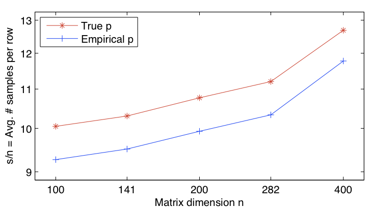
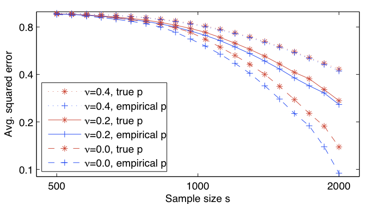
Figure 1: (a) Left: Sample size needed to obtain avg. error $0.1$, with respect to $n$. (b) Right: Excess error level over a range of sample sizes, for fixed $n=200$. (Axes are on a logarithmic scale.)

5 Discussion

In this paper, we prove learning guarantees for the weighted trace-norm by analyzing expected Rademacher complexities. We show that weighting with smoothed marginals eliminates degenerate scenarios that can arise in the case of a non-product sampling distribution, and demonstrate in experiments on the Netflix and MovieLens datasets that this correction can be useful in applied settings. We also give results for empirically-weighted trace-norm regularization, and see indications that using the empirical distribution may be better than using the true distribution, even if it is available.

Appendix A Proofs for the i.i.d. sampling setting

A.1 Proof of Theorem 1

We first fill in the details for the Rademacher bound in the case that $p$ has uniform row- and column-marginals. Define

$$Q_{t}=\sigma_{t}\frac{e_{i_{t},j_{t}}}{\sqrt{p^{r}\left({i_{t}}\right)p^{c}\left({j_{t}}\right)}}\in\mathbb{R}^{n\times m}\;.$$

We need to calculate $R$ and $\sigma^{2}$ such that $\left\lVert{Q_{t}}\right\rVert_{\mathrm{sp}}\leq R$ (almost surely) and

$$\sigma^{2}=\max\left\{\left\lVert{\sum{{\mbox{\bf E}}\left[{Q_{t}^{T}Q_{t}}\right]}}\right\rVert_{\mathrm{sp}},\left\lVert{\sum{{\mbox{\bf E}}\left[{Q_{t}Q^{T}_{t}}\right]}}\right\rVert_{\mathrm{sp}}\right\}.$$

For each $t$, $Q_{t}$ is just a matrix with a single non-zero entry of magnitude $\frac{1}{\sqrt{p^{r}\left({i}\right)p^{c}\left({j}\right)}}$, for some $i,j$, and so $\left\lVert{Q_{t}}\right\rVert_{\mathrm{sp}}\leq\max_{ij}\frac{1}{\sqrt{p^{r}\left({i}\right)p^{c}\left({j}\right)}}\doteq R$.

The matrix $Q_{t}Q_{t}^{T}\in\mathbb{R}^{n\times n}$ is equal to $\frac{e_{i,i}}{p^{r}\left({i}\right)p^{c}\left({j}\right)}$ with probability $p\left({i},{j}\right)$. Hence ${{\mbox{\bf E}}\left[{Q_{t}^{T}Q_{t}}\right]}$ is a diagonal matrix with entries $\sum_{j}\frac{p\left({i},{j}\right)}{p^{r}\left({i}\right)p^{c}\left({j}\right)}$. Similar arguments apply to $Q_{t}^{T}Q_{t}$. Multiplying by $s$, and recalling the spectral norm of a diagonal matrix is simply the maximal magnitude element, we have:

$$\sigma^{2}=s\cdot\max\left\{\max_{i}\sum_{j}\frac{p\left({i},{j}\right)}{p^{r}\left({i}\right)p^{c}\left({j}\right)},\max_{j}\sum_{i}\frac{p\left({i},{j}\right)}{p^{r}\left({i}\right)p^{c}\left({j}\right)}\right\}\;.$$

This completes the proof for the case that $p$ has uniform row- and column- marginals.

Next we turn to the case that $p$ is a product distribution, $p=p^{r}\times p^{c}$ (with possibly non-uniform marginals). For any $X\in\mathcal{W}_{r}\left[{p}\right]$, define

$$Z(X)=\left(X_{ij}\mathbb{I}\left\{{p\left({i},{j}\right)\geq\frac{\log(n)}{s\sqrt{nm}}}\right\}\right)_{ij}\;.$$

Let $\mathcal{Z}=\left\{Z(X):X\in\mathcal{W}_{r}\left[{p}\right]\right\}$.

We can then follow the proof of the bound in the uniform-marginals case, with a modified definition of $Q_{t}$:

$$Q_{t}=\sigma_{t}\frac{e_{i_{t},j_{t}}\mathbb{I}\left\{{p\left({i_{t}},{j_{t}}\right)\geq\frac{\log(n)}{s\sqrt{nm}}}\right\}}{\sqrt{p^{r}\left({i_{t}}\right)p^{c}\left({j_{t}}\right)}}\;.$$

Proceeding as in the proof for Theorem 1, we obtain $R\leq\sqrt{\frac{s\sqrt{nm}}{\log(n)}}$ and $\sigma^{2}\leq sn$, and thus

$${{\mbox{\bf E}}_{S\sim p}\left[{\hat{\mathcal{R}}_{S}(\mathcal{Z})}\right]}=\mathbf{O}\left(\sqrt{\frac{rn\log(n)}{s}}\right)\;.$$

Therefore, by [13],

$${{\mbox{\bf E}}\left[{\sup_{X\in\mathcal{W}_{r}\left[{p}\right]}L_{p}(Z(X))-\hat{L}_{S}(Z(X))}\right]}\leq\mathbf{O}\left(l\cdot\sqrt{\frac{rn\log(n)}{s}}\right)\;,$$

$${{\mbox{\bf E}}\left[{\sup_{X\in\mathcal{W}_{r}\left[{p}\right]}\hat{L}_{S}(Z(X))-L_{p}(Z(X))}\right]}\leq\mathbf{O}\left(l\cdot\sqrt{\frac{rn\log(n)}{s}}\right)\;.$$

Next, let $I=\left(\sqrt{p\left({i},{j}\right)}\mathbb{I}\left\{{p\left({i},{j}\right)<\frac{\log(n)}{s\sqrt{nm}}}\right\}\right)_{ij}$. For any matrix $M$, define

$$\left\|{M}\right\|_{F\left(p^{r},p^{c}\right)}=\left\|{\mathrm{diag}\left({p^{r}}\right)^{\nicefrac{{1}}{{2}}}M\mathrm{diag}\left({p^{c}}\right)^{\nicefrac{{1}}{{2}}}}\right\|_{F}\;.$$

Now take any $M$ with $\left\|{M}\right\|_{F\left(p^{r},p^{c}\right)}\leq 1$. Let $M^{\prime}=\mathrm{diag}\left({p^{r}}\right)^{\nicefrac{{1}}{{2}}}M\mathrm{diag}\left({p^{c}}\right)^{\nicefrac{{1}}{{2}}}$, then $\left\|{M^{\prime}}\right\|_{F}\leq 1$. We have

$$\sum_{ij:p\left({i},{j}\right)<\frac{\log(n)}{s\sqrt{nm}}}p\left({i},{j}\right)M_{ij}=\sum_{ij}I_{ij}M^{\prime}_{ij}=\langle I,M^{\prime}\rangle\leq\left\|{I}\right\|_{F}\cdot\left\|{M^{\prime}}\right\|_{F}$$

$$\leq\left\|{I}\right\|_{F}=\sqrt{\sum_{ij}p\left({i},{j}\right)\mathbb{I}\left\{{p\left({i},{j}\right)<\frac{\log(n)}{s\sqrt{nm}}}\right\}}\leq\sqrt{nm\cdot\frac{\log(n)}{s\sqrt{nm}}}=\sqrt{\frac{\sqrt{nm}\log(n)}{s}}\;.$$

Since $\left\|{M}\right\|_{F}\leq\left\|{M}\right\|_{\mathrm{tr}}$ for any matrix $M$, we then have, for any $X\in\mathcal{W}_{r}\left[{p}\right]$, $\left\|{X}\right\|_{F\left(p^{r},p^{c}\right)}\leq\left\|{X}\right\|_{\mathrm{tr}\left(p^{r},p^{c}\right)}\leq\sqrt{r}$, and so

$$\left|L_{p}(X)-L_{p}(Z(X))\right|=\left|\sum_{ij\not\in\mathcal{I}}p\left({i},{j}\right)\left(\ell(X_{ij},Y_{ij})-\ell(0,Y_{ij})\right)\right|$$

$$\leq l\cdot\sum_{ij\not\in\mathcal{I}}p\left({i},{j}\right)|X_{ij}|\leq\sqrt{\frac{l^{2}r\sqrt{nm}\log(n)}{s}}\;.$$

And, fixing some $X^{*}\in\mathcal{W}_{r}\left[{p}\right]$ such that $L_{p}(X^{*})=\inf_{X\in\mathcal{W}_{r}\left[{p}\right]}L_{p}(X)$,

$${{\mbox{\bf E}}\left[{\sup_{X\in\mathcal{W}_{r}\left[{p}\right]}\hat{L}_{S}(Z(X))-\hat{L}_{S}(X)}\right]}+{{\mbox{\bf E}}\left[{\hat{L}_{S}(X^{*})-\hat{L}_{S}(Z(X^{*}))}\right]}$$

$$={{\mbox{\bf E}}\left[{\sup_{X\in\mathcal{W}_{r}\left[{p}\right]}\frac{1}{s}\sum_{t=1}^{s}\mathbb{I}\left\{{(i_{t},j_{t})\not\in\mathcal{I}}\right\}\left(\ell(0,Y_{i_{t}j_{t}})-\ell(X_{i_{t}j_{t}},Y_{i_{t}j_{t}})\right)}\right]}$$

$$\ \ \ \ \ \ \ \ \ +{{\mbox{\bf E}}\left[{\frac{1}{s}\sum_{t=1}^{s}\mathbb{I}\left\{{(i_{t},j_{t})\not\in\mathcal{I}}\right\}\left(\ell(X^{*}_{i_{t}j_{t}},Y_{i_{t}j_{t}})-\ell(0,Y_{i_{t}j_{t}})\right)}\right]}$$

$$={{\mbox{\bf E}}\left[{\sup_{X\in\mathcal{W}_{r}\left[{p}\right]}\frac{1}{s}\sum_{t=1}^{s}\mathbb{I}\left\{{(i_{t},j_{t})\not\in\mathcal{I}}\right\}\left(\ell(X^{*}_{i_{t}j_{t}},Y_{i_{t}j_{t}})-\ell(X_{i_{t}j_{t}},Y_{i_{t}j_{t}})\right)}\right]}$$

$$\leq{{\mbox{\bf E}}\left[{\sup_{X\in\mathcal{W}_{r}\left[{p}\right]}\frac{1}{s}\sum_{t=1}^{s}\mathbb{I}\left\{{(i_{t},j_{t})\not\in\mathcal{I}}\right\}\ell(X^{*}_{i_{t}j_{t}},Y_{i_{t}j_{t}})}\right]}\leq l\cdot{{\mbox{\bf E}}\left[{\frac{1}{s}\sum_{t=1}^{s}\mathbb{I}\left\{{(i_{t},j_{t})\not\in\mathcal{I}}\right\}|X^{*}_{i_{t}j_{t}}|}\right]}$$

$$=l\cdot{{\mbox{\bf E}}\left[{\mathbb{I}\left\{{(i_{1},j_{1})\not\in\mathcal{I}}\right\}|X^{*}_{i_{1}j_{1}}|}\right]}=l\cdot\sum_{ij\not\in\mathcal{I}}p\left({i},{j}\right)|X^{*}_{ij}|\leq\sqrt{\frac{l^{2}r\sqrt{nm}\log(n)}{s}}$$

Then writing

$$L_{p}(\hat{X}_{S})-L_{p}(X^{*})=(L_{p}(\hat{X}_{S})-L_{p}(Z(\hat{X}_{S})))+(L_{p}(Z(\hat{X}_{S}))-\hat{L}_{S}(Z(\hat{X}_{S})))+(\hat{L}_{S}(Z(\hat{X}_{S}))-\hat{L}_{S}(\hat{X}_{S}))$$

$$+(\hat{L}_{S}(\hat{X}_{S})-\hat{L}_{S}(X^{*}))+(\hat{L}_{S}(X^{*})-\hat{L}_{S}(Z(X^{*})))+(\hat{L}_{S}(Z(X^{*}))-L_{p}(Z(X^{*})))+(L_{p}(Z(X^{*}))-L_{p}(X^{*}))\;,$$

we obtain

$${{\mbox{\bf E}}\left[{L_{p}(\hat{X}_{S})-L_{p}(X^{*})}\right]}\leq\mathbf{O}\left(\sqrt{\frac{l^{2}rn\log(n)}{s}}\right)\;.$$

A.2 Proof of Theorem 2

Assume $\ell$ is $l$-Lipschitz and $b$-bounded, and $r\geq 1$. We will show that (for any $p$)

$${{\mbox{\bf E}}_{S\sim p}\left[{\hat{\mathcal{R}}_{S}(\ell\circ\mathcal{W}_{r}\left[{p}\right])}\right]}=\mathbf{O}\left((l+b)\cdot\sqrt[3]{\frac{rn\log(n)}{s}}\right)\;.$$

Given a sample $S$, define

$$T^{0}_{S}=\left\{t\ :\ p^{r}\left({i_{t}}\right)\text{ or }p^{c}\left({j_{t}}\right)<\sqrt[3]{\frac{l^{2}r\log(n)}{b^{2}sn^{2}}}\right\}\;,T^{1}_{S}=\{1,\dots,s\}\backslash T^{0}_{S}\;.$$

We have

$$\hat{\mathcal{R}}_{S}(\ell\circ\mathcal{W}_{r}\left[{p}\right])={{\mbox{\bf E}}_{\sigma\sim\{\pm 1\}^{s}}\left[{\sup_{\left\|{X}\right\|_{\mathrm{tr}\left(p^{r},p^{c}\right)}\leq\sqrt{r}}\frac{1}{s}\sum_{t=1}^{s}\sigma_{t}\cdot\ell(X_{i_{t}j_{t}},Y_{i_{t}j_{t}})}\right]}$$

$$\leq{{\mbox{\bf E}}_{\sigma}\left[{\sup_{\left\|{X}\right\|_{\mathrm{tr}\left(p^{r},p^{c}\right)}\leq\sqrt{r}}\frac{1}{s}\sum_{t\in T^{0}_{S}}\sigma_{t}\cdot\ell(X_{i_{t}j_{t}},Y_{i_{t}j_{t}})}\right]}+{{\mbox{\bf E}}_{\sigma}\left[{\sup_{\left\|{X}\right\|_{\mathrm{tr}\left(p^{r},p^{c}\right)}\leq\sqrt{r}}\frac{1}{s}\sum_{t\in T^{1}_{S}}\sigma_{t}\cdot\ell(X_{i_{t}j_{t}},Y_{i_{t}j_{t}})}\right]}$$

Bounding the first term,

$${{\mbox{\bf E}}_{\sigma}\left[{\sup_{\left\|{X}\right\|_{\mathrm{tr}\left(p^{r},p^{c}\right)}\leq\sqrt{r}}\frac{1}{s}\sum_{t\in T^{0}_{S}}\sigma_{t}\cdot\ell(X_{i_{t}j_{t}},Y_{i_{t}j_{t}})}\right]}\leq{{\mbox{\bf E}}_{\sigma}\left[{\frac{1}{s}\sum_{t\in T^{0}_{S}}\left|\sigma_{t}\right|\cdot b}\right]}=\frac{b}{s}\cdot\left|T^{0}_{S}\right|\;.$$

In expectation over $S$,

$${{\mbox{\bf E}}_{S}\left[{\frac{b}{s}\cdot\left|T^{0}_{S}\right|}\right]}=b\cdot{{\mbox{\bf E}}_{ij\sim p}\left[{\mathbb{I}\left\{{p^{r}\left({i}\right)\text{ or }p^{c}\left({j}\right)<\sqrt[3]{\frac{l^{2}r\log(n)}{b^{2}sn^{2}}}}\right\}}\right]}$$

$$=b\cdot\sum_{ij}p\left({i},{j}\right)\mathbb{I}\left\{{p^{r}\left({i}\right)\text{ or }p^{c}\left({j}\right)<\sqrt[3]{\frac{l^{2}r\log(n)}{b^{2}sn^{2}}}}\right\}$$

$$\leq\left[b\cdot\sum_{i:p^{r}\left({i}\right)<\sqrt[3]{\frac{l^{2}r\log(n)}{b^{2}sn^{2}}}}\sum_{j}p\left({i},{j}\right)\right]+\left[b\cdot\sum_{j:p^{c}\left({j}\right)<\sqrt[3]{\frac{l^{2}r\log(n)}{b^{2}sn^{2}}}}\sum_{i}p\left({i},{j}\right)\right]$$

$$=\left[b\cdot\sum_{i:p^{r}\left({i}\right)<\sqrt[3]{\frac{l^{2}r\log(n)}{b^{2}sn^{2}}}}p^{r}\left({i}\right)\right]+\left[b\cdot\sum_{j:p^{c}\left({j}\right)<\sqrt[3]{\frac{l^{2}r\log(n)}{b^{2}sn^{2}}}}p^{c}\left({j}\right)\right]$$

$$\leq bn\cdot\sqrt[3]{\frac{l^{2}r\log(n)}{b^{2}sn^{2}}}+bm\sqrt[3]{\frac{l^{2}r\log(n)}{b^{2}sn^{2}}}\leq 2\sqrt[3]{\frac{l^{2}brn\log(n)}{s}}\;.$$

To bound the second term, we use the fact that $\left\|{\text{abs}(X)}\right\|_{\mathrm{tr}}\leq\left\|{X}\right\|_{\mathrm{tr}}$ for any matrix $X$, where $\text{abs}(X)$ is the matrix defined via $\text{abs}(X)_{ij}=|X_{ij}|$. We have

$${{\mbox{\bf E}}_{\sigma}\left[{\sup_{\left\|{X}\right\|_{\mathrm{tr}\left(p^{r},p^{c}\right)}\leq\sqrt{r}}\frac{1}{s}\sum_{t\in T^{1}_{S}}\sigma_{t}\cdot\ell(X_{i_{t}j_{t}},Y_{i_{t}j_{t}})}\right]}$$

$$\leq{{\mbox{\bf E}}_{\sigma}\left[{\sup_{\left\|{X}\right\|_{\mathrm{tr}\left(p^{r},p^{c}\right)}\leq\sqrt{r}}\frac{1}{s}\sum_{t\in T^{1}_{S}}\sigma_{t}\cdot\left(\ell(X_{i_{t}j_{t}},Y_{i_{t}j_{t}})-\ell(0,Y_{i_{t}j_{t}}\right)}\right]}+{{\mbox{\bf E}}_{\sigma}\left[{\sup_{\left\|{X}\right\|_{\mathrm{tr}\left(p^{r},p^{c}\right)}\leq\sqrt{r}}\frac{1}{s}\sum_{t\in T^{1}_{S}}\sigma_{t}\cdot\ell(0,Y_{i_{t}j_{t}})}\right]}$$

$$={{\mbox{\bf E}}_{\sigma}\left[{\sup_{\left\|{X}\right\|_{\mathrm{tr}\left(p^{r},p^{c}\right)}\leq\sqrt{r}}\frac{1}{s}\sum_{t\in T^{1}_{S}}\sigma_{t}\cdot\left(\ell(X_{i_{t}j_{t}},Y_{i_{t}j_{t}})-\ell(0,Y_{i_{t}j_{t}}\right)}\right]}\leq l\cdot{{\mbox{\bf E}}_{\sigma}\left[{\sup_{\left\|{X}\right\|_{\mathrm{tr}\left(p^{r},p^{c}\right)}\leq\sqrt{r}}\frac{1}{s}\sum_{t\in T^{1}_{S}}\sigma_{t}\cdot|X_{i_{t}j_{t}}|}\right]}$$

$$=l\cdot{{\mbox{\bf E}}_{\sigma}\left[{\sup_{\left\|{X^{\prime}}\right\|_{\mathrm{tr}}\leq\sqrt{r}}\frac{1}{s}\sum_{t\in T^{1}_{S}}\frac{\sigma_{t}}{\sqrt{p^{r}\left({i_{t}}\right)p^{c}\left({j_{t}}\right)}}\cdot|X^{\prime}_{i_{t}j_{t}}|}\right]}\leq l\cdot{{\mbox{\bf E}}_{\sigma}\left[{\sup_{\left\|{X^{\prime\prime}}\right\|_{\mathrm{tr}}\leq\sqrt{r}}\frac{1}{s}\sum_{t\in T^{1}_{S}}\frac{\sigma_{t}}{\sqrt{p^{r}\left({i_{t}}\right)p^{c}\left({j_{t}}\right)}}\cdot X^{\prime\prime}_{i_{t}j_{t}}}\right]}$$

$$=l\sqrt{r}\cdot{{\mbox{\bf E}}_{\sigma}\left[{\left\lVert{\frac{1}{s}\sum_{t=1}^{s}\sigma_{t}\frac{e_{(i_{t},j_{t})}\mathbb{I}\left\{{p^{r}\left({i_{t}}\right),p^{c}\left({j_{t}}\right)\geq\sqrt[3]{\frac{l^{2}r\log(n)}{b^{2}sn^{2}}}}\right\}}{\sqrt{p^{r}\left({i_{t}}\right)p^{c}\left({j_{t}}\right)}}}\right\rVert_{\mathrm{sp}}}\right]}\;,$$

Defining $Q_{t}=\sigma_{t}\frac{e_{(i_{t},j_{t})}\mathbb{I}\left\{{p^{r}\left({i_{t}}\right),p^{c}\left({j_{t}}\right)\geq\sqrt[3]{\frac{l^{2}r\log(n)}{b^{2}sn^{2}}}}\right\}}{\sqrt{p^{r}\left({i_{t}}\right)p^{c}\left({j_{t}}\right)}}$, we can follow identical arguments as in the proof of the first bound of this theorem. We have

$$\left\lVert{Q_{t}}\right\rVert_{\mathrm{sp}}\leq\max_{ij}\frac{\mathbb{I}\left\{{p^{r}\left({i}\right),p^{c}\left({j}\right)\geq\sqrt[3]{\frac{l^{2}r\log(n)}{b^{2}sn^{2}}}}\right\}}{\sqrt{p^{r}\left({i}\right)p^{c}\left({j}\right)}}\leq\sqrt[3]{\frac{b^{2}sn^{2}}{l^{2}r\log(n)}}\doteq R\;,$$

and

$$\sigma^{2}\doteq\max\left\{\left\lVert{\sum{{\mbox{\bf E}}\left[{Q_{t}^{T}Q_{t}}\right]}}\right\rVert_{\mathrm{sp}},\left\lVert{\sum{{\mbox{\bf E}}\left[{Q_{t}Q^{T}_{t}}\right]}}\right\rVert_{\mathrm{sp}}\right\}$$

$$\leq s\cdot\max\left\{\max_{i}\sum_{j}\frac{p\left({i},{j}\right)\mathbb{I}\left\{{p^{r}\left({i}\right),p^{c}\left({j}\right)\geq\sqrt[3]{\frac{l^{2}r\log(n)}{b^{2}sn^{2}}}}\right\}}{p^{r}\left({i}\right)p^{c}\left({j}\right)},\right.$$

$$\left.\hskip 142.26378pt\max_{j}\sum_{i}\frac{p\left({i},{j}\right)\mathbb{I}\left\{{p^{r}\left({i}\right),p^{c}\left({j}\right)\geq\sqrt[3]{\frac{l^{2}r\log(n)}{b^{2}sn^{2}}}}\right\}}{p^{r}\left({i}\right)p^{c}\left({j}\right)}\right\}$$

$$\leq s\cdot\sqrt[3]{\frac{b^{2}sn^{2}}{l^{2}r\log(n)}}\cdot\max\left\{\max_{i}\sum_{j}\frac{p\left({i},{j}\right)}{p^{r}\left({i}\right)},\max_{j}\sum_{i}\frac{p\left({i},{j}\right)}{p^{r}\left({i}\right)}\right\}=\sqrt[3]{\frac{b^{2}s^{4}n^{2}}{l^{2}r\log(n)}}$$

Then applying [14], we get

$${{\mbox{\bf E}}_{\sigma}\left[{\sup_{\left\|{X}\right\|_{\mathrm{tr}\left(p^{r},p^{c}\right)}\leq\sqrt{r}}\frac{1}{s}\sum_{t\in T^{1}_{S}}\sigma_{t}\cdot\ell(X_{i_{t}j_{t}},Y_{i_{t}j_{t}})}\right]}=\frac{l\sqrt{r}}{s}{{\mbox{\bf E}}_{S,\sigma}\left[{\left\lVert{\sum_{t=1}^{s}Q_{t}}\right\rVert_{\mathrm{sp}}}\right]}$$

$$\leq\mathbf{O}\left(\frac{l\sqrt{r}}{s}\left(\sigma\sqrt{\log(n)}+R\log(n)\right)\right)$$

$$\leq\mathbf{O}\left(\frac{l\sqrt{r}}{s}\left(\sqrt[6]{\frac{b^{2}s^{4}n^{2}}{l^{2}r\log(n)}}\sqrt{\log(n)}+\sqrt[3]{\frac{b^{2}sn^{2}}{l^{2}r\log(n)}}\log(n)\right)\right)$$

$$\leq\mathbf{O}\left(l^{\nicefrac{{2}}{{3}}}b^{\nicefrac{{1}}{{3}}}\sqrt[3]{\frac{rn\log(n)}{s}}+l^{\nicefrac{{1}}{{3}}}b^{\nicefrac{{2}}{{3}}}\left(\sqrt[3]{\frac{rn\log(n)}{s}}\right)^{2}\right)\;.$$

If $s\geq rn\log(n)$, then this proves the bound. If not, then the result is trivial, since $L_{p}(X)\leq b$ for any $X$.

A.3 Proof of Theorem 4

Throughout this section, assume $s\geq 24n\log(n)$. (If this is not the case, then we only need to prove excess error $\leq\mathbf{O}(l\sqrt{r})$, which is trivial given the class $\mathcal{W}_{r}\left[{\check{p}}\right]$.) We also assume $s\leq\mathbf{O}\left(nm\log(nm)\right)$. (If this is not the case, then with high probability, we observe all entries of the matrix and obtain optimal recovery.) The lemmas which are cited in this proof, are proved below.

Define

$$X^{*}=\arg\min_{X\in\mathcal{W}_{r}\left[{\tilde{p}}\right]}L_{p}(X),\ \ \ \ \ r^{*}=\left\|{X^{*}}\right\|_{\mathrm{tr}\left(p^{r},p^{c}\right)}^{2}\leq r\;.$$

For any sample $S$, define

$$c(S)=\max\left\{0,\left\|{\frac{1}{\sqrt{r^{*}}}X^{*}}\right\|_{\mathrm{tr}\left(\check{p}^{r},\check{p}^{c}\right)}-1\right\}\;.$$

Then, for a fixed $S$,

$$\left\|{(1-c(S))X^{*}}\right\|_{\mathrm{tr}\left(\check{p}^{r},\check{p}^{c}\right)}=\sqrt{r^{*}}(1-c(S))\left\|{\frac{1}{\sqrt{r^{*}}}X^{*}}\right\|_{\mathrm{tr}\left(\tilde{p}^{r},\tilde{p}^{c}\right)}\leq\sqrt{r}\ \Rightarrow\ (1-c(S))X^{*}\in\mathcal{W}_{r}\left[{\check{p}}\right]\;.$$

Applying Lemma 1 and Theorem 3,

$${{\mbox{\bf E}}\left[{L_{p}(\hat{X}_{S})-\hat{L}_{S}(\hat{X}_{S})}\right]}\leq{{\mbox{\bf E}}\left[{\sup_{X\in{\mathcal{W}_{r}\left[{\check{p}}\right]}}\left(L_{p}(X)-\hat{L}_{S}(X)\right)}\right]}$$

$$\leq{{\mbox{\bf E}}\left[{\sup_{X\in 2\cdot{\mathcal{W}_{r}\left[{\tilde{p}}\right]}}\left(L_{p}(X)-\hat{L}_{S}(X)\right)}\right]}+\frac{8\sqrt{l^{2}rnm}}{n^{2}}\leq\mathbf{O}\left(\sqrt{\frac{l^{2}rn\log(n)}{s}}\right)+\frac{8\sqrt{l^{2}rnm}}{n^{2}}$$

$$\leq\mathbf{O}\left(\sqrt{\frac{l^{2}rn\log(n)}{s}}\right)\;.$$

And, similarly,

$${{\mbox{\bf E}}\left[{\hat{L}_{S}((1-c(S))X^{*})-L_{p}((1-c(S))X^{*})}\right]}\leq{{\mbox{\bf E}}\left[{\sup_{X\in{\mathcal{W}_{r}\left[{\check{p}}\right]}}\left(\hat{L}_{S}(X)-L_{p}(X)\right)}\right]}$$

$$\leq{{\mbox{\bf E}}\left[{\sup_{X\in 2\cdot{\mathcal{W}_{r}\left[{\tilde{p}}\right]}}\left(\hat{L}_{S}(X)-L_{p}(X)\right)}\right]}+\frac{8\sqrt{l^{2}rnm}}{n^{2}}\leq\mathbf{O}\left(\sqrt{\frac{l^{2}rn\log(n)}{s}}\right)+\frac{8\sqrt{l^{2}rnm}}{n^{2}}$$

$$\leq\mathbf{O}\left(\sqrt{\frac{l^{2}rn\log(n)}{s}}\right)\;.$$

By definition, since $(1-c(S))X^{*}\in\mathcal{W}_{r}\left[{\check{p}}\right]$,

$${{\mbox{\bf E}}\left[{\hat{L}_{S}(\hat{X}_{S})-\hat{L}_{S}((1-c(S))X^{*})}\right]}\leq 0\;.$$

Finally, by Lemma 3,

$${{\mbox{\bf E}}\left[{L_{p}((1-c(S))X^{*})-L_{p}(X^{*})}\right]}\leq\sqrt{\frac{2l^{2}rn}{s}}\;.$$

Combining all of the above, we get

$${{\mbox{\bf E}}\left[{L_{p}(\hat{X}_{S})-L_{p}(X^{*})}\right]}\leq O\left(\sqrt{\frac{l^{2}rn\log(n)}{s}}\right)\;.$$

A.3.1 Lemmas for Theorem 6

Lemma 1.

$${{\mbox{\bf E}}\left[{\sup_{X\in{\mathcal{W}_{r}\left[{\check{p}}\right]}}\left(L_{p}(X)-\hat{L}_{S}(X)\right)}\right]}\leq{{\mbox{\bf E}}\left[{\sup_{X\in 2\cdot{\mathcal{W}_{r}\left[{\tilde{p}}\right]}}\left(L_{p}(X)-\hat{L}_{S}(X)\right)}\right]}+\frac{8\sqrt{l^{2}rnm}}{n^{2}}\;.$$

$${{\mbox{\bf E}}\left[{\sup_{X\in{\mathcal{W}_{r}\left[{\check{p}}\right]}}\left(\hat{L}_{S}(X)-L_{p}(X)\right)}\right]}\leq{{\mbox{\bf E}}\left[{\sup_{X\in 2\cdot{\mathcal{W}_{r}\left[{\tilde{p}}\right]}}\left(\hat{L}_{S}(X)-L_{p}(X)\right)}\right]}+\frac{8\sqrt{l^{2}rnm}}{n^{2}}\;.$$

Proof.

By Lemma 2, with probability at least $1-2n^{-2}$, for all $i,j$,

$$\check{p}^{r}\left({i}\right)\geq\frac{1}{2}\tilde{p}^{r}\left({i}\right),\ \check{p}^{c}\left({j}\right)\geq\frac{1}{2}\tilde{p}^{c}\left({j}\right)\;.$$

Let $A$ be the event that these inequalities hold. If $A$ occurs, then for any $X\in\mathcal{W}_{r}\left[{\check{p}}\right]$,

$$\left\|{X}\right\|_{\mathrm{tr}\left(p^{r},p^{c}\right)} =\left\|{\mathrm{diag}\left({\tilde{p}^{r}\left({i}\right)}\right)^{\nicefrac{{1}}{{2}}}X\mathrm{diag}\left({\tilde{p}^{c}\left({j}\right)}\right)^{\nicefrac{{1}}{{2}}}}\right\|_{\mathrm{tr}}$$

$$=\left\|{\mathrm{diag}\left({\frac{\tilde{p}^{r}\left({i}\right)}{\check{p}^{r}\left({i}\right)}}\right)^{\nicefrac{{1}}{{2}}}\mathrm{diag}\left({\check{p}^{r}\left({i}\right)}\right)^{\nicefrac{{1}}{{2}}}X\mathrm{diag}\left({\check{p}^{c}\left({j}\right)}\right)^{\nicefrac{{1}}{{2}}}\mathrm{diag}\left({\frac{\tilde{p}^{c}\left({j}\right)}{\check{p}^{c}\left({j}\right)}}\right)^{\nicefrac{{1}}{{2}}}}\right\|_{\mathrm{tr}}$$

$$\leq 2\left\|{\mathrm{diag}\left({\check{p}^{r}\left({i}\right)}\right)^{\nicefrac{{1}}{{2}}}X\mathrm{diag}\left({\check{p}^{c}\left({j}\right)}\right)^{\nicefrac{{1}}{{2}}}}\right\|_{\mathrm{tr}}=2\left\|{X}\right\|_{\mathrm{tr}\left(\check{p}^{r},\check{p}^{c}\right)}\leq 2\sqrt{r}\;.$$

In this case, $\mathcal{W}_{r}\left[{\check{p}}\right]\subset 2\cdot\mathcal{W}_{r}\left[{\tilde{p}}\right]$, and therefore,

$$\sup_{X\in\mathcal{W}_{r}\left[{\check{p}}\right]}\left[\left(L_{p}(X)-L_{p}(\mathbf{0}_{n\times m})\right)-\left(\hat{L}_{S}(X)-\hat{L}_{S}(\mathbf{0}_{n\times m})\right)\right]$$

$$\leq\sup_{X\in 2\cdot\mathcal{W}_{r}\left[{\tilde{p}}\right]}\left[\left(L_{p}(X)-L_{p}(\mathbf{0}_{n\times m})\right)-\left(\hat{L}_{S}(X)-\hat{L}_{S}(\mathbf{0}_{n\times m})\right)\right]\;.$$

Next we consider the case that $A$ does not occur. For any $X\in\mathcal{W}_{r}\left[{\check{p}}\right]$,

$$|X|_{\infty} \leq\left\|{X}\right\|_{F}=2\sqrt{nm}\left\|{\mathrm{diag}\left({\frac{1}{2n}\mathbf{1}_{n}}\right)^{\nicefrac{{1}}{{2}}}X\mathrm{diag}\left({\frac{1}{2m}\mathbf{1}_{m}}\right)^{\nicefrac{{1}}{{2}}}}\right\|_{F}$$

$$\leq 2\sqrt{nm}\left\|{\mathrm{diag}\left({\frac{1}{2n}\mathbf{1}_{n}}\right)^{\nicefrac{{1}}{{2}}}X\mathrm{diag}\left({\frac{1}{2m}\mathbf{1}_{m}}\right)^{\nicefrac{{1}}{{2}}}}\right\|_{\mathrm{tr}}\leq 2\sqrt{nm}\left\|{X}\right\|_{\mathrm{tr}\left(\check{p}^{r},\check{p}^{c}\right)}\leq 2\sqrt{rnm}\;.$$

Therefore,

$$\sup_{X\in\mathcal{W}_{r}\left[{\check{p}}\right]}\left[\left(L_{p}(X)-L_{p}(\mathbf{0}_{n\times m})\right)-\left(\hat{L}_{S}(X)-\hat{L}_{S}(\mathbf{0}_{n\times m})\right)\right]$$

$$\leq\sup_{X\in\mathcal{W}_{r}\left[{\check{p}}\right]}\left[\sum_{ij}p\left({i},{j}\right)\left(\ell(X_{ij},Y_{ij})-\ell(0,Y_{ij})\right)-\frac{1}{s}\sum_{t}\left(\ell(X_{i_{t}j_{t}},Y_{i_{t}j_{t}})-\ell(0,Y_{i_{t}j_{t}})\right)\right]$$

$$\leq l\cdot\sup_{X\in\mathcal{W}_{r}\left[{\check{p}}\right]}\left[\sum_{ij}p\left({i},{j}\right)\cdot|X_{ij}|+\frac{1}{s}\sum_{t}|X_{i_{t}j_{t}}|\right]$$

$$\leq l\cdot\sup_{X\in\mathcal{W}_{r}\left[{\check{p}}\right]}\left[\sum_{ij}p\left({i},{j}\right)\cdot 2\sqrt{rnm}+\frac{1}{s}\sum_{t}2\sqrt{rnm}\right]\leq 4\sqrt{l^{2}rnm}$$

And so,

$${{\mbox{\bf E}}_{S}\left[{\sup_{X\in\mathcal{W}_{r}\left[{\check{p}}\right]}\left[\left(L_{p}(X)-L_{p}(\mathbf{0}_{n\times m})\right)-\left(\hat{L}_{S}(X)-\hat{L}_{S}(\mathbf{0}_{n\times m})\right)\right]}\right]}$$

$$={{\mbox{\bf E}}_{S}\left[{\sup_{X\in\mathcal{W}_{r}\left[{\check{p}}\right]}\left[\left(L_{p}(X)-L_{p}(\mathbf{0}_{n\times m})\right)-\left(\hat{L}_{S}(X)-\hat{L}_{S}(\mathbf{0}_{n\times m})\right)\right]\cdot\mathbb{I}\left\{{A}\right\}}\right]}$$

$$\ \ \ \ \ \ +{{\mbox{\bf E}}_{S}\left[{\sup_{X\in\mathcal{W}_{r}\left[{\check{p}}\right]}\left[\left(L_{p}(X)-L_{p}(\mathbf{0}_{n\times m})\right)-\left(\hat{L}_{S}(X)-\hat{L}_{S}(\mathbf{0}_{n\times m})\right)\right]\cdot\mathbb{I}\left\{{A^{c}}\right\}}\right]}$$

$$\leq{{\mbox{\bf E}}_{S}\left[{\sup_{X\in 2\cdot\mathcal{W}_{r}\left[{\tilde{p}}\right]}\left[\left(L_{p}(X)-L_{p}(\mathbf{0}_{n\times m})\right)-\left(\hat{L}_{S}(X)-\hat{L}_{S}(\mathbf{0}_{n\times m})\right)\right]\cdot\mathbb{I}\left\{{A}\right\}}\right]}+P\left(A^{c}\right)\cdot 4\sqrt{l^{2}rnm}$$

$$\leq{{\mbox{\bf E}}_{S}\left[{\sup_{X\in 2\cdot\mathcal{W}_{r}\left[{\tilde{p}}\right]}\left[\left(L_{p}(X)-L_{p}(\mathbf{0}_{n\times m})\right)-\left(\hat{L}_{S}(X)-\hat{L}_{S}(\mathbf{0}_{n\times m})\right)\right]\cdot\mathbb{I}\left\{{A}\right\}}\right]}+\frac{8\sqrt{l^{2}rnm}}{n^{2}}$$

$$\leq{{\mbox{\bf E}}_{S}\left[{\sup_{X\in 2\cdot\mathcal{W}_{r}\left[{\tilde{p}}\right]}\left[\left(L_{p}(X)-L_{p}(\mathbf{0}_{n\times m})\right)-\left(\hat{L}_{S}(X)-\hat{L}_{S}(\mathbf{0}_{n\times m})\right)\right]}\right]}+\frac{8\sqrt{l^{2}rnm}}{n^{2}}\;.$$

where the last step is true because, since $\mathbf{0}_{n\times m}\in 2\cdot\mathcal{W}_{r}\left[{\tilde{p}}\right]$, for any $S$,

$$\sup_{X\in 2\cdot\mathcal{W}_{r}\left[{\tilde{p}}\right]}\left[\left(L_{p}(X)-L_{p}(\mathbf{0}_{n\times m})\right)-\left(\hat{L}_{S}(X)-\hat{L}_{S}(\mathbf{0}_{n\times m})\right)\right]\geq 0\;.$$

And, ${{\mbox{\bf E}}_{S}\left[{L_{p}(\mathbf{0}_{n\times m})-\hat{L}_{S}(\mathbf{0}_{n\times m})}\right]}=0$, so therefore,

$${{\mbox{\bf E}}_{S}\left[{\sup_{X\in{\mathcal{W}_{r}\left[{\check{p}}\right]}}\left(L_{p}(X)-\hat{L}_{S}(X)\right)}\right]}\leq{{\mbox{\bf E}}\left[{\sup_{X\in 2\cdot{\mathcal{W}_{r}\left[{\tilde{p}}\right]}}\left(L_{p}(X)-\hat{L}_{S}(X)\right)}\right]}+\frac{8\sqrt{l^{2}rnm}}{n^{2}}\;.$$

The second claim can be proved with identical arguments. ∎

Lemma 2.

With probability at least $1-2n^{-2}$, for all $i$ and all $j$,

$$\check{p}^{r}\left({i}\right)\geq\frac{1}{2}\tilde{p}^{r}\left({i}\right),\ \check{p}^{c}\left({j}\right)\geq\frac{1}{2}\tilde{p}^{c}\left({j}\right)\;.$$

Proof.

Take any row $i$. Suppose that $p^{r}\left({i}\right)\leq\frac{1}{n}$. Then $\tilde{p}^{r}\left({i}\right)\leq\frac{1}{n}$, while $\check{p}^{r}\left({i}\right)=\frac{1}{2}\left(\hat{p}^{r}\left({i}\right)+\frac{1}{n}\right)\geq\frac{1}{2n}$. Therefore, in this case, $\check{p}^{r}\left({i}\right)\geq\frac{1}{2}\tilde{p}^{r}\left({i}\right)$ with probability $1$.

Next, suppose that $p^{r}\left({i}\right)>\frac{1}{n}$. Then, by the Chernoff inequality,

$$P\left(\hat{p}^{r}\left({i}\right)<\frac{1}{2}p^{r}\left({i}\right)\right) =P\left(\mathrm{Bin}(s,p^{r}\left({i}\right))<sp^{r}\left({i}\right)\left(1-\frac{1}{2}\right)\right)\leq e^{-\frac{sp^{r}\left({i}\right)}{8}}$$

$$\leq e^{-\frac{s}{8n}}\leq e^{-3\log(n)}=n^{-3}\;.$$

Therefore, with probability at least $1-n^{-3}$, $\hat{p}^{r}\left({i}\right)\geq\frac{1}{2}p^{r}\left({i}\right)$, and so

$$\check{p}^{r}\left({i}\right) =\frac{1}{2}\left(\hat{p}^{r}\left({i}\right)+\frac{1}{n}\right)\geq\frac{1}{2}\left(\frac{1}{2}p^{r}\left({i}\right)+\frac{1}{n}\right)\geq\frac{1}{2}\tilde{p}^{r}\left({i}\right)\;.$$

Therefore, for any row $i$, with probability at least $1-n^{-3}$, $\check{p}^{r}\left({i}\right)\geq\frac{1}{2}\tilde{p}^{r}\left({i}\right)$. The same reasoning applies to every column $j$. Therefore, with probability at least $1-2n^{-2}$, the statement holds for all $i$ and all $j$. ∎

Lemma 3.

Fix $X^{*}$ with $\left\|{X^{*}}\right\|_{\mathrm{tr}\left(\tilde{p}^{r},\tilde{p}^{c}\right)}^{2}=r^{*}\leq r$, and define

$$c(S)=\max\left\{0,\left\|{\frac{1}{\sqrt{r^{*}}}X^{*}}\right\|_{\mathrm{tr}\left(\check{p}^{r},\check{p}^{c}\right)}-1\right\}\;.$$

Then

$${{\mbox{\bf E}}\left[{L_{p}((1-c(S))X^{*})-L_{p}(X^{*})}\right]}\leq\sqrt{\frac{2l^{2}rn}{s}}\;.$$

Proof.

$${L_{p}((1-c(S))X^{*})-L_{p}(X^{*})}=\sum_{ij}p\left({i},{j}\right)\left(\ell((1-c(S))X^{*}_{ij},Y_{ij})-\ell(X^{*}_{ij},Y_{ij})\right)$$

$$\leq l\cdot\sum_{ij}p\left({i},{j}\right)|(1-c(S))X^{*}_{ij}-X^{*}_{ij}|=l\cdot c(S)\cdot\sum_{ij}p\left({i},{j}\right)|X^{*}_{ij}|$$

$$=l\cdot c(S)\cdot\sum_{ij}\frac{p\left({i},{j}\right)}{\sqrt{\tilde{p}^{r}\left({i}\right)\tilde{p}^{c}\left({j}\right)}}\cdot\sqrt{\tilde{p}^{r}\left({i}\right)\tilde{p}^{c}\left({j}\right)}\cdot|X^{*}_{ij}|$$

Defining $M=\left(\frac{p\left({i},{j}\right)}{\sqrt{\tilde{p}^{r}\left({i}\right)\tilde{p}^{c}\left({j}\right)}}\right)_{ij}$,

$$=l\cdot c(S)\cdot\langle M,\left(\mathrm{diag}\left({\tilde{p}^{r}\left({i}\right)}\right)^{\nicefrac{{1}}{{2}}}X^{*}\mathrm{diag}\left({\tilde{p}^{c}\left({j}\right)}\right)^{\nicefrac{{1}}{{2}}}\right)_{ij}\rangle$$

$$\leq l\cdot c(S)\cdot\left\lVert{M}\right\rVert_{\mathrm{sp}}\cdot\left\|{\left(\mathrm{diag}\left({\tilde{p}^{r}\left({i}\right)}\right)^{\nicefrac{{1}}{{2}}}X^{*}\mathrm{diag}\left({\tilde{p}^{c}\left({j}\right)}\right)^{\nicefrac{{1}}{{2}}}\right)_{ij}}\right\|_{\mathrm{tr}}$$

$$\leq l\sqrt{r}\cdot c(S)\cdot\left\lVert{M}\right\rVert_{\mathrm{sp}}\;.$$

Now we show that $\left\lVert{M}\right\rVert_{\mathrm{sp}}\leq 2$. Take any unit vectors $u\in\mathbb{R}^{m}$, $v\in\mathbb{R}^{n}$. Then

$$u^{T}Mv=\sum_{ij}p\left({i},{j}\right)\cdot\sqrt{\frac{u_{i}^{2}}{\tilde{p}^{r}\left({i}\right)}}\cdot\sqrt{\frac{v_{j}^{2}}{\tilde{p}^{c}\left({j}\right)}}\leq\frac{1}{2}\sum_{ij}p\left({i},{j}\right)\left(\frac{u_{i}^{2}}{\tilde{p}^{r}\left({i}\right)}+\frac{v_{j}^{2}}{\tilde{p}^{c}\left({j}\right)}\right)$$

$$=\frac{1}{2}\sum_{i}p^{r}\left({i}\right)\cdot\frac{u_{i}^{2}}{\tilde{p}^{r}\left({i}\right)}+\frac{1}{2}\sum_{j}p^{c}\left({j}\right)\cdot\frac{v_{j}^{2}}{\tilde{p}^{c}\left({j}\right)}\leq\frac{1}{2}\sum_{i}2u_{i}^{2}+\frac{1}{2}\sum_{j}2v_{j}^{2}=2\;.$$

So, by Lemma 4,

$${{\mbox{\bf E}}\left[{L_{p}((1-c(S))X^{*})-L_{p}(X^{*})}\right]}\leq 2l\sqrt{r}\cdot{{\mbox{\bf E}}\left[{c(S)}\right]}\leq 2l\sqrt{r}\cdot\sqrt{\frac{n}{2s}}\;.$$

∎

Lemma 4.

For any $p$, for any fixed $X$ with $\left\|{X}\right\|_{\mathrm{tr}\left(\tilde{p}^{r},\tilde{p}^{c}\right)}=1$,

$${{\mbox{\bf E}}\left[{\max\{0,\left\|{X}\right\|_{\mathrm{tr}\left(\check{p}^{r},\check{p}^{c}\right)}-1\}}\right]}\leq\sqrt{\frac{n}{2s}}\;.$$

Proof.

By properties of the trace-norm [5], we can write $\mathrm{diag}\left({\tilde{p}^{r}}\right)^{\nicefrac{{1}}{{2}}}X\mathrm{diag}\left({\tilde{p}^{c}}\right)^{\nicefrac{{1}}{{2}}}=AB^{T}$, where $\left\|{A}\right\|_{F}^{2}=\left\|{B}\right\|_{F}^{2}=\left\|{X}\right\|_{\mathrm{tr}\left(p^{r},p^{c}\right)}=1$. Define

$$D_{1}=\mathrm{diag}\left({\check{p}^{r}}\right)\mathrm{diag}\left({\tilde{p}^{r}}\right)^{-1},\ D_{2}=\mathrm{diag}\left({\check{p}^{c}}\right)\mathrm{diag}\left({\tilde{p}^{c}}\right)^{-1}\;.$$

Then, by properties of the trace-norm [5],

$$\left\|{X}\right\|_{\mathrm{tr}\left(\check{p}^{r},\check{p}^{c}\right)}=\left\|{\mathrm{diag}\left({\check{p}^{r}}\right)^{\nicefrac{{1}}{{2}}}X\mathrm{diag}\left({\check{p}^{c}}\right)^{\nicefrac{{1}}{{2}}}}\right\|_{\mathrm{tr}}=\left\|{\left(D_{1}^{\nicefrac{{1}}{{2}}}A\right)\left(D_{2}^{\nicefrac{{1}}{{2}}}B\right)^{T}}\right\|_{\mathrm{tr}}$$

$$\leq\frac{1}{2}\left\|{D_{1}^{\nicefrac{{1}}{{2}}}A}\right\|_{F}^{2}+\frac{1}{2}\left\|{D_{2}^{\nicefrac{{1}}{{2}}}B}\right\|_{F}^{2}$$

$$=\frac{1}{2}\sum_{i}\frac{\check{p}^{r}\left({i}\right)}{\tilde{p}^{r}\left({i}\right)}\|A_{(i)}\|_{2}^{2}+\frac{1}{2}\sum_{j}\frac{\check{p}^{c}\left({j}\right)}{\tilde{p}^{c}\left({j}\right)}\|B_{(j)}\|^{2}_{2}$$

$$=\frac{1}{4}\sum_{i}\frac{\hat{p}^{r}\left({i}\right)+\frac{1}{n}}{\tilde{p}^{r}\left({i}\right)}\|A_{(i)}\|_{2}^{2}+\frac{1}{4}\sum_{j}\frac{\hat{p}^{c}\left({j}\right)+\frac{1}{m}}{\tilde{p}^{c}\left({j}\right)}\|B_{(j)}\|^{2}_{2}$$

$$=\frac{1}{4}\sum_{i}\frac{N^{r}_{i}+\frac{s}{n}}{s\tilde{p}^{r}\left({i}\right)}\|A_{(i)}\|_{2}^{2}+\frac{1}{4}\sum_{j}\frac{N^{c}_{j}+\frac{s}{m}}{s\tilde{p}^{c}\left({j}\right)}\|B_{(j)}\|^{2}_{2}\;,$$

where $N^{r}_{i}$ is the number of samples in row $i$, and $N^{c}_{j}$ is the number of samples in column $j$. Clearly,

$${{\mbox{\bf E}}\left[{\frac{1}{4}\sum_{i}\frac{N^{r}_{i}+\frac{s}{n}}{s\tilde{p}^{r}\left({i}\right)}\|A_{(i)}\|_{2}^{2}+\frac{1}{4}\sum_{j}\frac{N^{c}_{j}+\frac{s}{m}}{s\tilde{p}^{c}\left({j}\right)}\|B_{(j)}\|^{2}_{2}}\right]}$$

$$=\frac{1}{4}\sum_{i}\frac{sp^{r}\left({i}\right)+\frac{s}{n}}{s\tilde{p}^{r}\left({i}\right)}\|A_{(i)}\|_{2}^{2}+\frac{1}{4}\sum_{j}\frac{sp^{c}\left({j}\right)+\frac{s}{m}}{s\tilde{p}^{c}\left({j}\right)}\|B_{(j)}\|^{2}_{2}$$

$$=\frac{1}{4}\sum_{i}\frac{2s\tilde{p}^{r}\left({i}\right)}{s\tilde{p}^{r}\left({i}\right)}\|A_{(i)}\|_{2}^{2}+\frac{1}{4}\sum_{j}\frac{2s\tilde{p}^{c}\left({j}\right)}{s\tilde{p}^{c}\left({j}\right)}\|B_{(j)}\|^{2}_{2}$$

$$=\frac{1}{2}\left\|{A}\right\|_{F}^{2}+\frac{1}{2}\left\|{B}\right\|_{F}^{2}=1\;.$$

And, we can compute

$$\text{Var}(N^{r}_{i})\leq sp^{r}\left({i}\right),\ \text{Cov}(N^{r}_{i},N^{r}_{i^{\prime}})<0,\ \text{Var}(N^{c}_{j})\leq sp^{c}\left({j}\right),\ \text{Cov}(N^{c}_{j},N^{c}_{j^{\prime}})<0\;.$$

Therefore,

$$\text{Var}\left(\sum_{i}\frac{N^{r}_{i}}{s\tilde{p}^{r}\left({i}\right)}\|A_{(i)}\|^{2}_{2}+\sum_{j}\frac{N^{c}_{j}}{s\tilde{p}^{c}\left({j}\right)}\|B_{(j)}\|^{2}_{2}\right)$$

$$\leq 2\text{Var}\left(\sum_{i}\frac{N^{r}_{i}}{s\tilde{p}^{r}\left({i}\right)}\|A_{(i)}\|^{2}_{2}\right)+2\text{Var}\left(\sum_{j}\frac{N^{c}_{j}}{s\tilde{p}^{c}\left({j}\right)}\|B_{(j)}\|^{2}_{2}\right)$$

$$=\sum_{i}\frac{1}{s^{2}\tilde{p}^{r}\left({i}\right)^{2}}\text{Var}(N^{r}_{i})\|A_{(i)}\|^{4}_{2}+2\sum_{i<i^{\prime}}\frac{1}{s^{2}\tilde{p}^{r}\left({i}\right)\tilde{p}^{r}\left({i^{\prime}}\right)}\text{Cov}(N^{r}_{i},N^{r}_{i^{\prime}})\|A_{(i)}\|^{2}_{2}\|A_{(i^{\prime})}\|^{2}_{2}$$

$$\ \ \ \ +\sum_{j}\frac{1}{s^{2}\tilde{p}^{c}\left({j}\right)}\text{Var}(N^{c}_{j})\|B_{(j)}\|^{4}_{2}+2\sum_{j<j^{\prime}}\frac{1}{s^{2}\tilde{p}^{c}\left({j}\right)\tilde{p}^{c}\left({j^{\prime}}\right)}\text{Cov}(N^{c}_{j},N^{c}_{j^{\prime}})\|B_{(j)}\|^{2}_{2}\|B_{(j^{\prime})}\|^{2}_{2}$$

$$\leq\sum_{i}\frac{1}{s^{2}\tilde{p}^{r}\left({i}\right)^{2}}\text{Var}(N^{r}_{i})\|A_{(i)}\|^{4}_{2}+\sum_{j}\frac{1}{s^{2}\tilde{p}^{c}\left({j}\right)}\text{Var}(N^{c}_{j})\|B_{(j)}\|^{4}_{2}$$

$$\leq\sum_{i}\frac{sp^{r}\left({i}\right)}{s^{2}\tilde{p}^{r}\left({i}\right)^{2}}\|A_{(i)}\|^{4}_{2}+\sum_{j}\frac{sp^{c}\left({j}\right)}{s^{2}\tilde{p}^{c}\left({j}\right)}\|B_{(j)}\|^{4}_{2}$$

Since $\tilde{p}^{r}\left({i}\right)\geq\frac{1}{2}p^{r}\left({i}\right)$ and $\tilde{p}^{r}\left({i}\right)\geq\frac{1}{2n}$, and similarly for the columns, we continue:

$$\leq\sum_{i}\frac{4n}{s}\|A_{(i)}\|^{4}_{2}+\sum_{j}\frac{4m}{s}\|B_{(j)}\|^{4}_{2}\leq\frac{4n}{s}\left(\sum_{i}\|A_{(i)}\|^{2}_{2}\right)^{2}+\frac{4m}{s}\left(\sum_{j}\|B_{(j)}\|^{2}_{2}\right)$$

$$\leq\frac{4n}{s}\left\|{A}\right\|_{F}^{4}+\frac{4m}{s}\left\|{B}\right\|_{F}^{4}\leq\frac{4(n+m)}{s}\;.$$

So, we have

$${{\mbox{\bf E}}\left[{\max\{0,\left\|{X}\right\|_{\mathrm{tr}\left(\check{p}^{r},\check{p}^{c}\right)}-1\}}\right]}$$

$$\leq{{\mbox{\bf E}}\left[{\max\left\{0,\frac{1}{4}\sum_{i}\frac{N^{r}_{i}+\frac{s}{n}}{s\tilde{p}^{r}\left({i}\right)}\|A_{(i)}\|_{2}^{2}+\frac{1}{4}\sum_{j}\frac{N^{c}_{j}+\frac{s}{m}}{s\tilde{p}^{c}\left({j}\right)}\|B_{(j)}\|^{2}_{2}-1\right\}}\right]}$$

$$\leq\sqrt{\text{Var}\left(\frac{1}{4}\sum_{i}\frac{N^{r}_{i}+\frac{s}{n}}{s\tilde{p}^{r}\left({i}\right)}\|A_{(i)}\|_{2}^{2}+\frac{1}{4}\sum_{j}\frac{N^{c}_{j}+\frac{s}{m}}{s\tilde{p}^{c}\left({j}\right)}\|B_{(j)}\|^{2}_{2}\right)}$$

$$=\sqrt{\text{Var}\left(\frac{1}{4}\sum_{i}\frac{N^{r}_{i}}{s\tilde{p}^{r}\left({i}\right)}\|A_{(i)}\|_{2}^{2}+\frac{1}{4}\sum_{j}\frac{N^{c}_{j}}{s\tilde{p}^{c}\left({j}\right)}\|B_{(j)}\|^{2}_{2}\right)}\leq\sqrt{\frac{(n+m)}{4s}}$$

∎

Appendix B Proofs for the transductive setting

B.1 Proof of Theorem 5

Let $\overline{S}\subset[n]\times[m]$ be a subset of size $2s$. Let $\overline{p}$ denote the smoothed empirical marginals of $\overline{S}$.

Now choose any $S\subset\overline{S}$, a training set of size $s$. Without loss of generality, write $\overline{S}=\left\{(i_{1},j_{1}),\dots,(i_{2s},j_{2s})\right\}$ and $S=\left\{(i_{1},j_{1}),\dots,(i_{s},j_{s})\right\}$.

First, we bound transductive Rademacher complexity. By Lemma 12 in [5], for any sample $S$,

$$\hat{\mathcal{R}}_{S}(\mathcal{W}_{r}\left[{\overline{p}}\right]) ={{\mbox{\bf E}}_{\sigma\sim\{\pm 1\}^{s}}\left[{\sup_{X\in\mathcal{W}_{r}\left[{\overline{p}}\right]}\frac{1}{s}\sum_{t=1}^{s}\sigma_{t}X_{i_{t}j_{t}}}\right]}$$

$$={{\mbox{\bf E}}_{\sigma\sim\{\pm 1\}^{s}}\left[{\sup_{X\in\mathcal{W}_{r}\left[{\overline{p}}\right]}\frac{1}{s}\sum_{ij}X_{ij}\left(\sum_{t:(i_{t},j_{t})=(i,j)}\sigma_{t}\right)}\right]}$$

$$\leq{{\mbox{\bf E}}_{\sigma\sim\{\pm 1\}^{n\times m}}\left[{\sup_{X\in\mathcal{W}_{r}\left[{\overline{p}}\right]}\frac{1}{s}\sum_{ij}X_{ij}\sigma_{ij}\cdot\#\{t:(i_{t},j_{t})=(i,j),1\leq t\leq s\}}\right]}$$

$$={{\mbox{\bf E}}_{\sigma\sim\{\pm 1\}^{n\times m}}\left[{\sup_{X\in\mathcal{W}_{r}\left[{\overline{p}}\right]}\frac{1}{s}\sum_{ij}X_{ij}\sigma_{ij}\cdot\mathbb{I}\left\{{(i,j)\in S}\right\}}\right]}\;.$$

Now define matrix $\Sigma$ via

$$\Sigma_{ij}=\frac{\mathbb{I}\left\{{(i,j)\in S}\right\}}{s\sqrt{\overline{p}^{r}\left({i}\right)\overline{p}^{c}\left({j}\right)}}\;.$$

We have

$${{\mbox{\bf E}}_{S\sim p}\left[{\hat{\mathcal{R}}_{S}(\mathcal{W}_{r}\left[{\overline{p}}\right])}\right]} \leq{{\mbox{\bf E}}_{S}\left[{{{\mbox{\bf E}}_{\sigma\sim\{\pm 1\}^{n\times m}}\left[{\sup_{X\in\mathcal{W}_{r}\left[{\overline{p}}\right]}\frac{1}{s}\sum_{ij}X_{ij}\sigma_{ij}\cdot\mathbb{I}\left\{{(i,j)\in S}\right\}}\right]}}\right]}$$

$$={{\mbox{\bf E}}_{S}\left[{{{\mbox{\bf E}}_{\sigma\sim\{\pm 1\}^{n\times m}}\left[{\sup_{X\in\mathcal{W}_{r}\left[{\overline{p}}\right]}\sum_{ij}\left(\sqrt{p^{r}\left({i}\right)}X_{ij}\sqrt{p^{c}\left({j}\right)}\right)\sigma_{ij}\Sigma_{ij}}\right]}}\right]}$$

$$={{\mbox{\bf E}}_{S}\left[{{{\mbox{\bf E}}_{\sigma\sim\{\pm 1\}^{n\times m}}\left[{\sup_{X:\left\|{X}\right\|_{\mathrm{tr}}\leq\sqrt{r}}X_{ij}\sigma_{ij}\Sigma_{ij}}\right]}}\right]}$$

$$=\sqrt{r}\cdot{{\mbox{\bf E}}_{S}\left[{{{\mbox{\bf E}}_{\sigma\sim\{\pm 1\}^{n\times m}}\left[{\left\lVert{\sigma\bullet\Sigma}\right\rVert_{\mathrm{sp}}}\right]}}\right]}\;,$$

where $\sigma\bullet\Sigma$ is the element-wise product of $\Sigma$ with the random sign matrix $\sigma=(\sigma_{ij})$. By [20],

$${{\mbox{\bf E}}_{\sigma\sim\{\pm 1\}^{n\times m}}\left[{\left\lVert{\sigma\bullet\Sigma}\right\rVert_{\mathrm{sp}}}\right]}\leq\mathbf{O}\left(\log^{1/4}(n+m)\right)\cdot\max\left\{\max_{i}\left\lVert{\Sigma_{(i)}}\right\rVert_{2},\max_{j}\left\lVert{\Sigma^{(j)}}\right\rVert_{2}\right\}\;.$$

We now bound $\left\lVert{\Sigma_{(i)}}\right\rVert_{2}$ and $\left\lVert{\Sigma^{(j)}}\right\rVert_{2}$. Fix any $i$. Then

$$\left\lVert{\Sigma_{(i)}}\right\rVert_{2}^{2}=\sum_{j}\Sigma_{ij}^{2}=\sum_{j=1}^{m}\frac{\mathbb{I}\left\{{(i,j)\in S}\right\}}{\left(s\overline{p}^{r}\left({i}\right)\right)\cdot\left(s\overline{p}^{c}\left({j}\right)\right)}\leq\sum_{j=1}^{m}\frac{\mathbb{I}\left\{{(i,j)\in\overline{S}}\right\}}{\left(s\overline{p}^{r}\left({i}\right)\right)\cdot\left(s\cdot\frac{1}{2m}\right)}$$

$$\leq\sum_{j=1}^{m}\frac{\#\{t:(i_{t},j_{t})=(i,j),1\leq t\leq 2s\}}{\left(\frac{1}{4}\#\left\{t:i_{t}=i,1\leq t\leq 2s\right\}\right)\cdot\left(s\cdot\frac{1}{2m}\right)}\leq\frac{\#\{t:i_{t}=i,1\leq t\leq 2s\}}{\left(\frac{1}{4}\#\left\{t:i_{t}=i,1\leq t\leq 2s\right\}\right)\cdot\left(s\cdot\frac{1}{2m}\right)}\leq\frac{8m}{s}\;.$$

Similarly, for all $j$, $\left\lVert{\Sigma^{(j)}}\right\rVert_{2}^{2}\leq\frac{8n}{s}$. Therefore,

$${{\mbox{\bf E}}_{S\sim p}\left[{\hat{\mathcal{R}}_{S}(\mathcal{W}_{r}\left[{\overline{p}}\right])}\right]}\leq\sqrt{r}\cdot{{\mbox{\bf E}}_{S}\left[{{{\mbox{\bf E}}_{\sigma\sim\{\pm 1\}^{n\times m}}\left[{\left\lVert{\sigma\bullet\Sigma}\right\rVert_{\mathrm{sp}}}\right]}}\right]}$$

$$\leq\sqrt{r}\cdot{{\mbox{\bf E}}_{S}\left[{\mathbf{O}\left(\log^{1/4}(n)\right)\cdot\max\left\{\max_{i}\left\lVert{\Sigma_{(i)}}\right\rVert_{2},\max_{j}\left\lVert{\Sigma^{(j)}}\right\rVert_{2}\right\}}\right]}\leq\mathbf{O}\left(\sqrt{\frac{rn\log^{\nicefrac{{1}}{{2}}}(n)}{s}}\right)\;.$$

Applying Theorem 5 of [12] (using integration to obtain a bound in expectation from a bound in probability),

$${{\mbox{\bf E}}_{S}\left[{\hat{L}_{\overline{S}\backslash S}(\hat{X}_{S})-\inf_{X\in\mathcal{W}_{r}\left[{\overline{p}}\right]}\hat{L}_{\overline{S}\backslash S}(X)}\right]}\leq\mathbf{O}\left(\sqrt{\frac{l^{2}rn\log^{\nicefrac{{1}}{{2}}}(n)+b^{2}}{s}}\right)\;.$$

B.2 Transductive version of Theorem 1

Let $\overline{p}$ now denote the (unsmoothed) empirical marginals of $\overline{S}$. If $\overline{p}^{r}\left({i}\right)\geq\frac{1}{Cn}$ and $\overline{p}^{c}\left({j}\right)\geq\frac{1}{Cm}$ for all $i,j$, defining

$$\hat{X}_{S}=\arg\min_{X\in\mathcal{W}_{r}\left[{\overline{p}}\right]}\hat{L}_{S}(X)\;,$$

we can then show that, for an $l$-Lipschitz loss $\ell$ bounded by $b$, in expectation over the split of $\overline{S}$ into training set $S$ and test set $T$,

$$\hat{L}_{T}(\hat{X}_{S})\leq\inf_{X\in\mathcal{W}_{r}\left[{\overline{p}}\right]}\hat{L}_{T}(X)+\mathbf{O}\left(C^{\nicefrac{{1}}{{2}}}l\cdot\sqrt{\frac{rn\log^{\nicefrac{{1}}{{2}}}(n)+b^{2}}{s}}\right)\;.$$

We prove this by following identical arguments as in the proof of Theorem 5, we define

$$\Sigma_{ij}=\frac{\mathbb{I}\left\{{(i,j)\in S}\right\}}{s\sqrt{\overline{p}^{r}\left({i}\right)\overline{p}^{c}\left({j}\right)}}\;,$$

and obtain $\left\lVert{\Sigma_{(i)}}\right\rVert_{2}^{2},\left\lVert{\Sigma^{(j)}}\right\rVert_{2}^{2}\leq\frac{2Cn}{s}$ for all $i,j$, which yields

$${{\mbox{\bf E}}_{S}\left[{\hat{L}_{\overline{S}\backslash S}(\hat{X}_{S})-\inf_{X\in\mathcal{W}_{r}\left[{\overline{p}}\right]}\hat{L}_{\overline{S}\backslash S}(X)}\right]}\leq\mathbf{O}\left(\sqrt{\frac{Cl^{2}rn\log^{\nicefrac{{1}}{{2}}}(n)+b^{2}}{s}}\right)\;.$$

In fact, we can obtain the same result with a weaker requirement on $\overline{p}$, namely

$$\frac{s}{n}\max\left\{\max_{i}\|\Sigma_{(i)}\|^{2}_{2},\max_{j}\|\Sigma^{(j)}\|^{2}_{2}\right\}\leq\max\left\{\max_{i}\frac{1}{m}\sum_{j=1}^{m}\frac{\frac{1}{s}\mathbb{I}\left\{{(i,j)\in\overline{S}}\right\}}{\overline{p}^{r}\left({i}\right)\overline{p}^{c}\left({j}\right)},\max_{j}\frac{1}{n}\sum_{i=1}^{n}\frac{\frac{1}{s}\mathbb{I}\left\{{(i,j)\in\overline{S}}\right\}}{\overline{p}^{r}\left({i}\right)\overline{p}^{c}\left({j}\right)}\right\}\leq C\;.$$

For instance, this quantity is likely to be bounded if $\overline{S}$ is a sample drawn from a product distribution on the matrix.

B.3 Transductive version of Theorem 2

Let $\overline{p}$ now denote the (unsmoothed) empirical marginals of $\overline{S}$. We define

$$\hat{X}_{S}=\arg\min_{X\in\mathcal{W}_{r}\left[{\overline{p}}\right]}\hat{L}_{S}(X)\;,$$

we can then show that, for an $l$-Lipschitz loss $\ell$ bounded by $b$, without any requirements on $\overline{p}$, in expectation over the split of $\overline{S}$ into training set $S$ and test set $T$,

$$\hat{L}_{T}(\hat{X}_{S})\leq\inf_{X\in\mathcal{W}_{r}\left[{\overline{p}}\right]}\hat{L}_{T}(X)+\mathbf{O}\left((l+b)\cdot\sqrt[3]{\frac{rn\log(n)}{s}}\right)\;.$$

We prove this by combining the proof techniques used in the proofs of Theorems 2 and 5. Define

$$T^{0}_{S}=\left\{t\ :\ 1\leq t\leq 2s,p^{r}\left({i_{t}}\right)\text{ or }p^{c}\left({j_{t}}\right)<\sqrt[3]{\frac{l^{2}r\log(n)}{b^{2}sn^{2}}}\right\}\;,T^{1}_{S}=\{1,\dots,2s\}\backslash T^{0}_{S}\;.$$

We then have

$$\hat{\mathcal{R}}_{S}(\ell\circ\mathcal{W}_{r}\left[{\overline{p}}\right])={{\mbox{\bf E}}_{\sigma\sim\{\pm 1\}^{s}}\left[{\sup_{X\in\mathcal{W}_{r}\left[{\overline{p}}\right]}\frac{1}{s}\sum_{t=1}^{s}\sigma_{t}\ell(X_{i_{t}j_{t}},Y_{i_{t}j_{t}})}\right]}$$

$$\leq{{\mbox{\bf E}}_{\sigma\sim\{\pm 1\}^{n\times m}}\left[{\sup_{X\in\mathcal{W}_{r}\left[{\overline{p}}\right]}\frac{1}{s}\sum_{ij}\ell(X_{i_{t}j_{t}},Y_{i_{t}j_{t}})\sigma_{ij}\cdot\mathbb{I}\left\{{(i,j)\in S}\right\}}\right]}$$

$$\leq{{\mbox{\bf E}}_{\sigma}\left[{\sup_{X\in\mathcal{W}_{r}\left[{\overline{p}}\right]}\frac{1}{s}\sum_{ij}\ell(X_{i_{t}j_{t}},Y_{i_{t}j_{t}})\sigma_{ij}\cdot\mathbb{I}\left\{{(i,j)\in S,\text{ and }\overline{p}^{r}\left({i}\right),\overline{p}^{c}\left({j}\right)\geq\sqrt[3]{\frac{l^{2}r\log(n)}{b^{2}sn^{2}}}}\right\}}\right]}$$

$$\ \ \ \ \ +{{\mbox{\bf E}}_{\sigma}\left[{\sup_{X\in\mathcal{W}_{r}\left[{\overline{p}}\right]}\frac{1}{s}\sum_{ij}\ell(X_{i_{t}j_{t}},Y_{i_{t}j_{t}})\sigma_{ij}\cdot\mathbb{I}\left\{{(i,j)\in S,\text{ and }\overline{p}^{r}\left({i}\right)\text{ or }\overline{p}^{c}\left({j}\right)<\sqrt[3]{\frac{l^{2}r\log(n)}{b^{2}sn^{2}}}}\right\}}\right]}$$

$$\doteq\text{(Term 1)}+\text{(Term 2)};.$$

Now define matrix $\Sigma$ via

$$\Sigma_{ij}=\frac{\mathbb{I}\left\{{(i,j)\in S,\text{ and }\overline{p}^{r}\left({i}\right),\overline{p}^{c}\left({j}\right)\geq\sqrt[3]{\frac{l^{2}r\log(n)}{b^{2}sn^{2}}}}\right\}}{s\sqrt{\overline{p}^{r}\left({i}\right)\overline{p}^{c}\left({j}\right)}}\;.$$

Following the same arguments as in the proof of Theorem 5, we obtain for all $i,j$,

$$\|\Sigma_{(i)}\|^{2}_{2},\|\Sigma^{(j)}\|^{2}_{2}\leq\frac{4}{s}\cdot\sqrt[3]{\frac{b^{2}sn^{2}}{l^{2}r\log(n)}}$$

Therefore, using the same arguments as in the proof of Theorem 2,

$$\text{(Term 1)}\leq l\sqrt{r}\mathbf{O}\left(\log^{\nicefrac{{1}}{{4}}}(n)\sqrt{\frac{4}{s}\cdot\sqrt[3]{\frac{b^{2}sn^{2}}{l^{2}r\log(n)}}}\right)=\mathbf{O}\left(\sqrt[3]{\frac{l^{2}brn\log(n)}{s}}\right)\;.$$

Next we have

$$\text{(Term 2)}={{\mbox{\bf E}}_{\sigma}\left[{\sup_{X\in\mathcal{W}_{r}\left[{\overline{p}}\right]}\frac{1}{s}\sum_{ij}\ell(X_{i_{t}j_{t}},Y_{i_{t}j_{t}})\sigma_{ij}\cdot\mathbb{I}\left\{{(i,j)\in S,\text{ and }\overline{p}^{r}\left({i}\right)\text{ or }\overline{p}^{c}\left({j}\right)<\sqrt[3]{\frac{l^{2}r\log(n)}{b^{2}sn^{2}}}}\right\}}\right]}$$

$$\leq\sup_{X\in\mathcal{W}_{r}\left[{\overline{p}}\right]}\frac{1}{s}\sum_{ij}\ell(X_{i_{t}j_{t}},Y_{i_{t}j_{t}})\cdot\mathbb{I}\left\{{(i,j)\in S,\text{ and }\overline{p}^{r}\left({i}\right)\text{ or }\overline{p}^{c}\left({j}\right)<\sqrt[3]{\frac{l^{2}r\log(n)}{b^{2}sn^{2}}}}\right\}$$

$$\leq\frac{1}{s}\sum_{ij}b\cdot\mathbb{I}\left\{{(i,j)\in\overline{S},\text{ and }\overline{p}^{r}\left({i}\right)\text{ or }\overline{p}^{c}\left({j}\right)<\sqrt[3]{\frac{l^{2}r\log(n)}{b^{2}sn^{2}}}}\right\}$$

$$\leq\frac{1}{s}\sum_{i:\overline{p}^{r}\left({i}\right)<\sqrt[3]{\frac{l^{2}r\log(n)}{b^{2}sn^{2}}}}\left(\sum_{j:(i,j)\in\overline{S}}b\right)+\frac{1}{s}\sum_{j:\overline{p}^{c}\left({j}\right)<\sqrt[3]{\frac{l^{2}r\log(n)}{b^{2}sn^{2}}}}\left(\sum_{i:(i,j)\in\overline{S}}b\right)$$

$$\leq\frac{2n}{s}\left(b\cdot 2s\cdot\sqrt[3]{\frac{l^{2}r\log(n)}{b^{2}sn^{2}}}\right)\leq\mathbf{O}\left(\sqrt[3]{\frac{l^{2}rbn\log(n)}{s}}\right)\;.$$

Combining the two, we get $\mathcal{R}_{s}(\ell\circ\mathcal{W}_{r}\left[{\overline{p}}\right])\leq\mathbf{O}\left(\sqrt[3]{\frac{l^{2}rbn\log(n)}{s}}\right)$, and therefore, in expectation over the split of $\overline{S}$ into $S$ and $T$,

$$\hat{L}_{T}(\hat{X}_{S})\leq\inf_{X\in\mathcal{W}_{r}\left[{\overline{p}}\right]}\hat{L}_{T}(X)+\mathbf{O}\left((l+b)\cdot\sqrt[3]{\frac{rn\log(n)}{s}}\right)\;.$$

References

- Srebro et al. [2004] N. Srebro, J. Rennie, and T. Jaakkola. Maximum-margin matrix factorization. Advances in Neural Information Processing Systems, 17, 2004.
- Salakhutdinov and Mnih [2007] R. Salakhutdinov and A. Mnih. Probabilistic matrix factorization. Advances in Neural Information Processing Systems, 20, 2007.
- Bach [2008] F. Bach. Consistency of trace-norm minimization. Journal of Machine Learning Research, 9:1019–1048, 2008.
- Candès and Tao [2009] E. Candès and T. Tao. The power of convex relaxation: Near-optimal matrix completion. IEEE Trans. Inform. Theory, 56(5):2053–2080, 2009.
- Srebro and Shraibman [2005] N. Srebro and A. Shraibman. Rank, trace-norm and max-norm. 18th Annual Conference on Learning Theory (COLT), pages 545–560, 2005.
- Recht [2009] B. Recht. A simpler approach to matrix completion. arXiv:0910.0651, 2009.
- Keshavan et al. [2010] R. Keshavan, A. Montanari, and S. Oh. Matrix completion from noisy entries. Journal of Machine Learning Research, 11:2057–2078, 2010.
- Koltchinskii et al. [2010] V. Koltchinskii, A. Tsybakov, and K. Lounici. Nuclear norm penalization and optimal rates for noisy low rank matrix completion. arXiv:1011.6256, 2010.
- Negahban and Wainwright [2010] S. Negahban and M. Wainwright. Restricted strong convexity and weighted matrix completion: Optimal bounds with noise. arXiv:1009.2118, 2010.
- Foygel and Srebro [2011] R. Foygel and N. Srebro. Concentration-based guarantees for low-rank matrix reconstruction. 24th Annual Conference on Learning Theory (COLT), 2011.
- Salakhutdinov and Srebro [2010] R. Salakhutdinov and N. Srebro. Collaborative Filtering in a Non-Uniform World: Learning with the Weighted Trace Norm. Advances in Neural Information Processing Systems, 23, 2010.
- Shamir and Shalev-Shwartz [2011] O. Shamir and S. Shalev-Shwartz. Collaborative filtering with the trace norm: Learning, bounding, and transducing. 24th Annual Conference on Learning Theory (COLT), 2011.
- Bartlett and Mendelson [2002] P. Bartlett and S. Mendelson. Rademacher and Gaussian complexities: Risk bounds and structural results. Journal of Machine Learning Research, 3:463–482, 2002.
- Tropp [2010] J.A. Tropp. User-friendly tail bounds for sums of random matrices. arXiv:1004.4389, 2010.
- Bennett and Lanning [2007] J. Bennett and S. Lanning. The netflix prize. In Proceedings of KDD Cup and Workshop, volume 2007, page 35. Citeseer, 2007.
- Dataset [2006] MovieLens Dataset. Available at http://www.grouplens.org/node/73. 2006.
- Koren [2008] Yehuda Koren. Factorization meets the neighborhood: a multifaceted collaborative filtering model. ACM Int. Conference on Knowledge Discovery and Data Mining (KDD’08), pages 426–434, 2008.
- Lee et al. [2010] J. Lee, B. Recht, R. Salakhutdinov, N. Srebro, and J. Tropp. Practical Large-Scale Optimization for Max-Norm Regularization. Advances in Neural Information Processing Systems, 23, 2010.
- Mazumder et al. [2010] R. Mazumder, T. Hastie, and R. Tibshirani. Spectral regularization algorithms for learning large incomplete matrices. Journal of Machine Learning Research, 11:2287–2322, 2010.
- Seginer [2000] Y. Seginer. The expected norm of random matrices. Combinatorics, Probability and Computing, 9(2):149–166, 2000.