Eigenvalue and eigenspace anholonomies in hierarchical systems

Abstract

An adiabatic cycle of parameters in a quantum system can yield the quantum anholonomies, nontrivial evolution not just in phase of the states, but also in eigenvalues and eigenstates. Such exotic anholonomies imply that an adiabatic cycle rearranges eigenstates even without spectral degeneracy. We show that an arbitrarily large quantum circuit generated by recursive extension can also exhibit the eigenvalue and eigenspace anholonomies.

A quantum system described by a parametric Hamiltonian goes through an adiabatic change connecting instantaneous eigenstates when it is subjected to a slow variation of parameters. Berry pointed out that this adiabatic change can yield nontrivial anholonomy in quantum phase when the trajectory of the parameter variation is closed to form a loop, for which he coined the term geometric phase [1].

Anholonomy under cyclic adiabatic parameter variation need not be limited to the phase of an eigenstate, but can involve the interchange of eigenvalues and eigenstates, since what is required after the return to the original parameter value is the identity of the whole set of eigensystem. Curiously, however, this possibility has been overlooked until recently, when examples of quantum system exhibiting eigenvalue and eigenspace anholonomy have been found, first in the Hamiltonian spectra of one-dimensional system with generalized point interaction [2], and then in the Floquet spectra of time-periodic kicked-spin [3] (see also, Fig. 1). In hindsight, quantum anholonomy of Wilczek and Zee, in which eigenstates belonging to a single degenerate eigenvalue undergo mutual exchange and mixing [4], can be thought of as a precursor to this new type. Since then, further examples of novel type of quantum anholonomy have been found both in Hamiltonian [5, 6] and Floquet systems [7, 8]. In one example, even the requirement of adiabaticity has been lifted, and the new type of anholonomy is shown to persist in a system with non-adiabatic cyclic parameter variation [6].

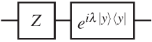
Figure 1: A simple quantum circuit that exhibits eigenvalue and eigenspace anholonomies, where $Z=|{}0{}\rangle\langle{}0{}|-|{}1{}\rangle\langle{}1{}|$ and $|{}y{}\rangle\equiv(|{}0{}\rangle-i|{}1{}\rangle)/{\sqrt{2}}$. Note that $e^{i{\lambda}|{}y{}\rangle\langle{}y{}|}$ is a phase shift gate: If the input is $|{}y{}\rangle$, this gate put a phase factor $e^{i\lambda}$ to the qubit. On the other hand, if the input state is orthogonal to $|{}y{}\rangle$, this gate do not change the state of the qubit. This system can be interpreted as a kicked spin system [3]. Although the eigenvalue and eigenspace anholonomies may be considered to be rather exotic, these anholonomies appear even in such a simple system. We will examine its $N$-qubit extensions in the main text.

Lately, it has been shown that all quantum holonomy, namely, Berry, Wilczek-Zee and the novel type having the eigenvalue exchange can be described by a unified formulation which is built upon the generalized Mead-Truhlar-Berry gauge connection [8]. The structure of gauge connection in the anholonomy of the new type has been examined in terms of the theory of Abelian gerbes [9]. It is also clarified that the exceptional point, the singularity of gauge connection in complex plane, plays a crucial role in the new type of quantum holonomy [10]. Applications to adiabatic manipulations of quantum states, including quantum computation [11], are promising [3, 12], since the eigenvalue and eigenspace anholonomies are stable against perturbations that retains the periodicity of the parameter space [3, 7].

Until now, there has been no known composite system that exhibits the new type of quantum anholonomy. In other words, all the conventional examples are “one-body” type systems. This raises the question on whether there is any way to realize the eigenvalue and eigenspace anholonomies in quantum composite systems. This question is not only fundamental for the anholonomies, but also important for the application to quantum computation [12]: It is essential to deal with more than one qubit and to find a systematic way to generate multi-qubit systems starting from a single qubit.

In this letter, we propose a systematic way to construct quantum circuits that exhibit the eigenvalue and eigenspace anholonomies based upon multiple qubits. The obtained multi-qubit systems clearly show that the hierarchical structure exists in the resultant quantum circuits. We also examine the influence of the hierarchical structure on the non-Abelian gauge connection associated with the eigenspace anholonomy.

1 Preliminaries — a one-body example

We first explain the constituent building block of our many-body examples. This is a quantum circuit on a qubit. The eigenvalue and eigenspace anholonomies in the constituent are also explained using a gauge theoretical approach for the anholonomies [8].

We introduce our simplest example (Fig. 1):

$$\hat{u}(\lambda)=e^{i\lambda|{}y{}\rangle\langle{}y{}|}\hat{Z},$$ (1)

where $\hat{X}\equiv|{}0{}\rangle\langle{}1{}|+\text{h.c.}$, $\hat{Y}\equiv i|{}1{}\rangle\langle{}0{}|+\text{h.c.}$, and $\hat{Z}\equiv|{}0{}\rangle\langle{}0{}|-|{}1{}\rangle\langle{}1{}|$. $|{}y{}\rangle\equiv(|{}0{}\rangle-i|{}1{}\rangle)/{\sqrt{2}}$ satisfies $\hat{Y}|{}y{}\rangle=-|{}y{}\rangle$. The first factor in Eq. (1) is the phase shift gate where the $y$-axis of the control qubit is chosen. We solve the eigenvalue problem of $\hat{u}(\lambda)$. Let $z(n;\lambda)$ denote the $n$-th eigenvalue of the unitary operator $\hat{u}(\lambda)$ ($n=0,1$). Since $z(n;\lambda)$ is a a unimodular complex number, we introduce a real number $\theta(n;\lambda)$ that satisfies $z(n;\lambda)=\exp\{i\theta(n;\lambda)\}$:

$$\theta(n;\lambda)=n\pi+\frac{\lambda}{2},$$ (2)

which is called an eigenangle. The corresponding eigenvectors are

$$\begin{split}|{}0;\lambda{}\rangle&\equiv\cos\frac{\lambda}{4}|{}0{}\rangle+\sin\frac{\lambda}{4}|{}1{}\rangle,\\ |{}1;\lambda{}\rangle&\equiv\cos\frac{\lambda}{4}|{}1{}\rangle-\sin\frac{\lambda}{4}|{}0{}\rangle,\end{split}$$ (3)

where the phases of the eigenvectors are chosen so as to simplify the following analysis.

$\hat{u}(\lambda)$ is periodic with $\lambda$, namely $\hat{u}(\lambda+2\pi)=\hat{u}(\lambda)$. Let $C$ denote the closed path of $\lambda$ from $\lambda=0$ to $2\pi$. Both the spectral set $\left\{e^{i\theta(n;\lambda)}\right\}_{n=0,1}$ and the set of projectors $\left\{|{}n;\lambda{}\rangle\langle{}n;\lambda{}|\right\}_{n=0,1}$ obey the same periodicity of $\hat{u}(\lambda)$. However, each eigenvalue $e^{i\theta(n;\lambda)}$ and each projector $|{}n;\lambda{}\rangle\langle{}n;\lambda{}|$ have a longer period. Namely, $\hat{u}(\lambda)$ exhibits eigenvalue and eigenspace anholonomies under adiabatic parametric change along the closed path $C$, where eigenvalues and eigenvectors are respectively exchanged.

We outline a theoretical framework for the eigenangle and eigenspace anholonomies using the one-body example $\hat{u}(\lambda)$. First, we examine the anholonomy in eigenangles. Using integers $s(n)$ and $r(n)$, the parametric dependence of eigenangle is arranged as

$$\theta(n;\lambda+2\pi)=\theta(s(n);\lambda)+2\pi r(n).$$ (4)

Namely, the $n$-th eigenangle arrives the $s(n)$-th eigenangle after a cycle $C$. On the other hand, $r(n)$ is “a winding number” of quasienergy (cf. It is shown that $\sum_{n}r(n)$ offers a topological character for the “Floquet operator” $\hat{u}(\lambda)$ [13]). We introduce a $2\times 2$ matrix $S(C)$ whose elements are defined as

$$\{S(C)\}_{n^{\prime},n}\equiv\delta_{n^{\prime},s(n)}.$$ (5)

From Eq. (2), we have $s(n)=\overline{n}$ and $r(n)=n$, where $\overline{0}=1$ and $\overline{1}=0$. Accordingly, the permutation matrix $\{S(C)\}_{n^{\prime},n}=\delta_{n^{\prime},\bar{n}}$ describes a cycle whose length is $2$.

Second, we examine the geometric phase factors associated with the adiabatic time evolution along the cycle $C$. We introduce a holonomy matrix $M(C)$ [8], whose $(n^{\prime},n)$-th elements is the overlapping integral $\langle{}n^{\prime};\lambda{}|{}n;\lambda+2\pi{}\rangle$, where $|{}n;\lambda{}\rangle$ is supposed to satisfy the parallel transport condition [14] along $C$ for the non-degenerate eigenspace, i.e., $\langle{}n;\lambda{}|\partial_{\lambda}|{}n;\lambda{}\rangle=0$. Due to the periodicity of $\hat{u}(\lambda)$, $|{}n;\lambda+2\pi{}\rangle$ is either parallel or perpendicular to $|{}n;\lambda{}\rangle$. In the former case, the diagonal elements of $M(C)$ are the Berry’s geometric phase factors [1]. The latter case implies the presence of the eigenvalue and eigenspace anholonomies and the off-diagonal elements provides Manini-Pistolesi’s gauge invariants [15]. It is worth to remark that the nodal-free geometric phase factors, which are the eigenvalues of $M(C)$, offers the geometric phases for both cases [16]. An extension of Fujikawa formalism for the geometric phase [17] offers a gauge covariant expression of $M(C)$ [8]:

$$M(C)=\mathop{\mathrm{exp}}_{\rightarrow}\left(-i\int_{C}A(\lambda)\upd\lambda\right)\mathop{\mathrm{exp}}_{\leftarrow}\left(i\int_{C}A^{\mathrm{D}}(\lambda)\upd\lambda\right),$$ (6)

where $\mathop{\mathrm{exp}}_{\leftarrow}$ and $\mathop{\mathrm{exp}}_{\rightarrow}$ are path-ordered and anti-path-ordered exponentials, respectively. Gauge connections $\{A(\lambda)\}_{n^{\prime},n}\equiv i\langle{}n^{\prime};\lambda{}|\partial_{\lambda}|{}n;\lambda{}\rangle$ and $A^{\mathrm{D}}(\lambda)\equiv\delta_{n^{\prime},n}\{A(\lambda)\}_{n^{\prime},n}$ are also introduced. The second factor in the right hand side of Eq. (6) describes time evolution in terms of adiabatic basis vectors $|{}n;\lambda(t){}\rangle$ [18] (see also, Eq. (3) in Ref. [8]). On the other hand, the first factor in Eq. (6) is introduced so as to incorporate the multiple-valuedness of $|{}n;\lambda{}\rangle$, which is nothing but the eigenspace anholonomy [8]. The gauge connection in our model (1), under the gauge specified by Eq. (3), is

$$A(\lambda)=\frac{1}{4}Y,\quad\text{where}\quad\begin{bmatrix}Y_{00}&Y_{01}\\ Y_{10}&Y_{11}\end{bmatrix}=\begin{bmatrix}0&-i\\ i&0\end{bmatrix},$$ (7)

which implies $A^{\mathrm{D}}(\lambda)=0$. Accordingly, we obtain $M(C)=-iY$, or, equivalently

$$\{M(C)\}_{n^{\prime},n}=\{S(C)\}_{n^{\prime},n}(-1)^{n}.$$ (8)

Namely, $M(C)$ is composed by two parts, the permutation matrix $S(C)$ and the phase factors $(-1)^{n}$.

2 Recursive construction of $N$-qubit circuit

A crucial ingredient of our $N$-body extension of $\hat{u}(\lambda)$ is the following “super-operator” $\hat{D}[\cdot]$

$$\hat{D}[\hat{U}]\equiv\hat{C}^{y}[\hat{U}](\hat{Z}\otimes\hat{1})$$ (9)

in which

$$\hat{C}^{y}[U]\equiv(\hat{1}-|{}y{}\rangle\langle{}y{}|)\otimes\hat{1}+|{}y{}\rangle\langle{}y{}|\otimes\hat{U}$$ (10)

is a controlled-unitary gate, where the “axis” of the control-bit is chosen to be in the “$y$-direction”.

In order to expose the one body quantum circuit $\hat{u}(\lambda)$ hidden in $\hat{D}[\cdot]$, we examine $\hat{D}[\cdot]$ with the global phase gate $e^{i\lambda}\hat{1}_{\mathrm{A}}$ for an ancilla, where $\hat{1}_{\mathrm{A}}$ is the identity operator of the ancilla: $\hat{D}[e^{i\lambda}\hat{1}_{\mathrm{A}}]=\hat{u}(\lambda)\otimes\hat{1}_{\mathrm{A}}.$ Namely, we may say that $\hat{u}(\lambda)$ is an extension of the global phase gate on an ancilla with $\hat{D}[\cdot]$. This interpretation suggests the following $N$-body extension.

A family of quantum circuits $\hat{U}^{(N)}(\lambda)$ on $N$-qubits is recursively defined in the following. For $N=1$, we set $\hat{U}^{(1)}(\lambda)=\hat{u}(\lambda)$, which is examined above. For $N>1$, we compose $\hat{U}^{(N)}(\lambda)$ from a $(N-1)$-qubit circuit $\hat{U}^{(N-1)}(\lambda)$, adding a qubit (Fig. 2):

$$\hat{U}^{(N)}(\lambda)\equiv\hat{D}[\hat{U}^{(N-1)}(\lambda)].$$ (11)

We depict the quantum circuit with $N=3$ in Fig. 3. It is worth pointing out the scalability of $\hat{U}^{(N)}(\lambda)$, i.e., only ${\rm poly}(N)$ quantum gates are required to construct $\hat{U}^{(N)}(\lambda)$.

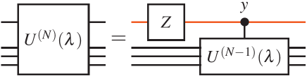
Figure 2: (Color online) Recursive construction of $\hat{U}^{(N)}(\lambda)$. The label $y$ over the control qubit indicates the “axis” for the control. $\hat{U}^{(N)}(\lambda)$ is made of a qubit, indicated by the uppermost line (colored), and $N-1$ qubits, indicated by the lower lines.

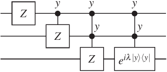
Figure 3: Circuit for $\hat{U}^{(3)}(\lambda)$. For notation, see, Fig. 2. The corresponding algebraic expression of the circuit is $\hat{U}^{(3)}(\lambda)=\{(\hat{C}^{y})^{2}[e^{i\lambda|{}y{}\rangle\langle{}y{}|}]\}\{(\hat{C}^{y})^{2}[Z]\}\{\hat{C}^{y}[Z]\}(Z\otimes 1\otimes 1),$ where $(\hat{C}^{y})^{n}[U]=\hat{C}^{y}[(\hat{C}^{y})^{n-1}[U]]$ for $n>1$ and $(\hat{C}^{y})^{1}[U]=\hat{C}^{y}[U]$. It is straightforward to see that $\hat{U}^{(N)}(\lambda)$ is composed by $Z$, $\hat{C}^{y}[Z]$, $\dots$, $(\hat{C}^{y})^{N-1}[Z]$ and $(\hat{C}^{y})^{N-1}[e^{i\lambda|{}y{}\rangle\langle{}y{}|}]$. Because $(\hat{C}^{y})^{n}[Z]$ can be composed by $\mathcal{O}(n^{2})$ quantum gates (see, e.g, §4.3 in Ref. [11]), $\hat{U}^{(N)}(\lambda)$ can be efficiently implemented by quantum gates.

We will solve the eigenvalue problem of $\hat{U}^{(N)}(\lambda)$. A complete set of quantum numbers for $\hat{U}^{(N)}(\lambda)$ is $(n_{N},n_{N-1},\cdots,n_{1})$, where $n_{j}\in\left\{0,1\right\}$. Let $|{}n_{N},n_{N-1},\cdots,n_{1};\lambda{}\rangle$ and $\theta^{(N)}(n_{N},n_{N-1},\cdots,n_{1};\lambda)$ denote an eigenvector and the corresponding eigenangle of $\hat{U}^{(N)}(\lambda)$, respectively. We will obtain recursion relations for eigenangles and eigenvectors. Suppose that we have an eigenvector $|{}\Psi{}\rangle$ and the corresponding eigenangle $\Theta$ of the smaller quantum circuit $\hat{U}^{(N-1)}(\lambda)$. From Eq. (11), $|{}n_{N};\Theta{}\rangle\otimes|{}\Psi{}\rangle$ is an eigenvector of $\hat{U}^{(N)}(\lambda)$, where $n_{N}\in\left\{0,1\right\}$. The corresponding eigenangle is $\theta^{(1)}(n_{N};\Theta)$. Accordingly the recursion relations are

$$\theta^{(N)}(n_{N},n_{N-1},\dots,n_{1};\lambda)$$

$$=\theta^{(1)}(n_{N};\theta^{(N-1)}(n_{N-1},\dots,n_{1};\lambda))$$ (12)

and

$$|{}n_{N},n_{N-1},\dots,n_{1};\lambda{}\rangle$$

$$=|{}n_{N};\theta^{(N-1)}(n_{N-1},\dots,n_{1};\lambda){}\rangle$$

$$\qquad\otimes|{}n_{N-1},\dots,n_{1};\lambda{}\rangle.$$ (13)

Hence we obtain the eigenangle

$$\theta^{(N)}(n_{N},\dots,n_{1};\lambda)$$

$$=\frac{2\pi}{2^{N}}\left\{m_{N}(n_{N},n_{N-1},\dots,n_{1})+\frac{\lambda}{2\pi}\right\},$$ (14)

where

$$m_{N}(n_{N},\dots,n_{1}) \equiv\sum_{j=1}^{N}2^{j-1}n_{j}.$$ (15)

This is called a principal quantum number. Note that $\hat{U}^{(N)}(\lambda)$ has no spectral degeneracy. Eq. (15) shows $n_{N},\dots,n_{1}$ are the coefficients of the binary expansion of $m_{N}$. Because of the simplicity of the correspondence between $m_{N}$ and $(n_{N},\dots,n_{1})$, we will identify them in the following. An eigenvector of $\hat{U}^{(N)}(\lambda)$ is

$$|{}n_{N},\dots,n_{1};\lambda{}\rangle$$

$$=|n_{N};\theta^{(N-1)}(m_{N-1};\lambda)\rangle\otimes\dots$$

$$\qquad\otimes|n_{2};\theta^{(1)}(m_{1};\lambda)\rangle\otimes|n_{1};\lambda\rangle.$$ (16)

3 Analysis of exotic anholonomies

We examine the parametric dependences of eigenangles and eigenprojectors of $\hat{U}^{(N)}(\lambda)$, along the cycle $C$, i.e., $\lambda\mapsto\lambda+2\pi$. Let $(n_{N},\dots,n_{1})$, or equivalently, $m_{N}$, be the set of quantum numbers of the initial eigenstate. After the completion of the parametric variation along the cycle $C$, the quantum numbers are rearranged, which shows the anholonomies take place. Let $s^{(N)}_{j}(m_{N};C)$ ($\in\left\{0,1\right\}$) denote the value of the $j$-th quantum number ($1\leq j\leq N$). We introduce a $2^{N}\times 2^{N}$ permutation matrix $S^{(N)}(C)$ whose elements are determined by $s^{(N)}_{j}(m_{N};C)$:

$$\{S^{(N)}(C)\}_{m^{\prime}_{N},m_{N}}=\prod_{j=1}^{N}\delta_{n^{\prime}_{j},s_{j}(m_{N};C)},$$ (17)

which represents an anholonomy in quantum numbers.

Now we show that $S^{(N)}(C)$ can be obtained from the parametric dependence of eigenangles:

$$\theta^{(N)}(m_{N};\lambda+2\pi)$$

$$=\theta^{(N)}(s^{(N)}(m_{N};C);\lambda)+2\pi r^{(N)}(m_{N};C),$$ (18)

where we abbreviate the collection of the quantum numbers $s^{(N)}_{N}(m_{N};C),\dots,s^{(N)}_{1}(m_{N};C)$ as $s^{(N)}(m_{N};C)$. An integer $r^{(N)}(m_{N};C)$ is a “winding number” of $\theta^{(N)}(m_{N};\lambda)$ in the periodic space of eigenangle.

In our model (Eq. (11)), $s^{(N)}_{N}$ and $r^{(N)}$ can be obtained through recursion relations. Here we show only the solutions:

$$s^{(N)}_{N}(n_{N},\dots,n_{1}) =\begin{cases}\overline{n_{N}}&\text{for $n_{N-1}\cdots n_{1}=1$}\\ n_{N}&\text{otherwise}\\ \end{cases},$$ (19)

and

$$r^{(N)}(n_{N},\dots,n_{1}) =n_{N}\cdots n_{1},$$ (20)

for $N>1$, and $s^{(1)}_{1}(n_{1})=\overline{n_{1}}$ and $r^{(1)}(n_{1})=n_{1}$. Hence the permutation matrix $S^{(N)}$ contains only a cycle whose length is $2^{N}$. The itinerary of $n_{N},\dots,n_{1}$ with $N=3$, for example, is the following

$$000\mapsto 001\mapsto 010\mapsto 011$$

$$\mapsto 100\mapsto 101\mapsto 110\mapsto 111\mapsto 000.$$ (21)

In terms of the principal quantum number $m_{N}$, this itinerary can be described in a simple way: When $m_{N}<2^{N}-1$, at every parametric variation of $\lambda$ by $2\pi$, $m_{N}$ increases by unity. Otherwise, $m_{N}$ becomes zero. Hence, after encircling the path $C$ by $2^{N}$ times, $m_{N}$ reruns to the initial point.

4 Adiabatic geometric phase

We examine the holonomy matrix

$$\{M^{(N)}(C)\}_{m^{\prime}_{N},m_{N}}=\langle{}m^{\prime}_{N};\lambda{}|{}\psi^{(C)}(m_{N};\lambda){}\rangle,$$ (22)

where $|{}\psi^{(C)}(m_{N};\lambda){}\rangle$ is obtained by the parallel transport of $|{}m_{N};\lambda{}\rangle$ along the path $C$. $M^{(N)}(C)$ incorporates two aspects of adiabatic cycle along $C$. One is the change in the quantum numbers, which is described by $S^{(N)}(C)$ (Eq. (17)). The other involves the geometric phase, in a generalized sense [15, 19]. Let $\sigma^{(N)}(m_{N})$ be the phase factor associated with the eigenspace initially labeled by $m_{N}$. These two factors comprise the holonomy matrix $\{M^{(N)}(C)\}_{m^{\prime}_{N},m_{N}}=\{S^{(N)}(C)\}_{m^{\prime}_{N},m_{N}}\sigma^{(N)}(m_{N};C).$ We will obtain the phase factor $\sigma^{(N)}(m_{N};C)$ using a gauge covariant expression of $M^{(N)}(C)$ (Eq. (6)). Here the non-Abelian gauge connection is

$$\{A^{(N)}(\lambda)\}_{m^{\prime}_{N},m_{N}}\equiv\langle{}m^{\prime}_{N};\lambda{}|\left[i\partial_{\lambda}|{}m_{N};\lambda{}\rangle\right].$$ (23)

Because of the absence of the spectral degeneracy in $\hat{U}^{(N)}(\lambda)$, the diagonal part of $A^{(N)}(\lambda)$ is $\{A^{\mathrm{D}(N)}(\lambda)\}_{m^{\prime}_{N},m_{N}}\equiv\delta_{m^{\prime}_{N},m_{N}}\{A^{(N)}(\lambda)\}_{m_{N},m_{N}}$.

We will obtain $A^{(N)}(\lambda)$ through recursion relations. Note that the results for the case $N=1$ are already obtained above. For $N>1$, the Leibniz rule in the derivative of Eq. (2) suggests the decomposition of the gauge connection $A^{(N)}(\lambda)=A^{(N)}_{\mathrm{H}}(\lambda)+A^{(N)}_{\mathrm{L}}(\lambda)$, where

$$\{A^{(N)}_{\mathrm{H}}(\lambda)\}_{m^{\prime}_{N},m_{N}}$$

$$\equiv\left\{A(\theta^{(N-1)}(m_{N-1}^{\prime};\lambda))\right\}_{n_{N}^{\prime},n_{N}}$$

$$\qquad{}\times\left\{\partial_{\lambda}\theta^{(N-1)}(m_{N-1}^{\prime};\lambda)\right\}\prod_{j=1}^{N-1}\delta_{n_{j}^{\prime},n_{j}}$$ (24)

$$\{A^{(N)}_{\mathrm{L}}(\lambda)\}_{m^{\prime}_{N},m_{N}}$$

$$\equiv\langle{}n^{\prime}_{N}(\theta^{(N-1)}(m_{N-1}^{\prime};\lambda)){}|{}n_{N}(\theta^{(N-1)}(m_{N-1};\lambda)){}\rangle$$

$$\qquad{}\times\left\{A^{(N-1)}(\lambda)\right\}_{m^{\prime}_{N-1},m_{N-1}}.$$ (25)

We also have a similar recursion relation for “diagonal” gauge connection $A^{\mathrm{D}(N)}(\lambda)$. As we have already chosen the gauge that satisfy $A^{\mathrm{D}}(\lambda)=0$ in the one-body problem, we obtain $A^{\mathrm{D}(N)}(\lambda)=0$ for all $N$ from the recursion relations. It is straightforward to obtain

$$A^{(N)}_{\mathrm{L}}(\lambda) =e^{i\pi 2^{-N}Y\otimes J_{\mathrm{D}}^{(N-1)}}\left\{1\otimes A^{(N-1)}(\lambda)\right\}$$

$$\qquad\times e^{-i\pi 2^{-N}Y\otimes J_{\mathrm{D}}^{(N-1)}},$$ (26)

and

$$A^{(N)}_{\mathrm{H}}(\lambda) =\frac{1}{2^{N+1}}Y\otimes 1^{(N-1)},$$ (27)

where $\left\{J_{\mathrm{D}}^{(N)}\right\}_{m^{\prime}_{N},m_{N}}\equiv m_{N}\delta_{m^{\prime}_{N},m_{N}}.$ Because $A^{(N)}_{\mathrm{H}}(\lambda)$ is independent of $\lambda$, $A^{(N)}_{\mathrm{L}}(\lambda)$ as well as $A^{(N)}(\lambda)$ are also independent of $\lambda$. Hence, in our model, $A^{(N)}(\lambda)$ is independent of $\lambda$. Furthermore, $A^{(N)}_{\mathrm{H}}(\lambda)$ commutes with $A^{(N)}_{\mathrm{L}}(\lambda)$. Now it is straightforward to obtain

$$\left\{M^{(N)}(C)\right\}_{m^{\prime}_{N},m_{N}} =\{S^{(N)}(C)\}_{m^{\prime}_{N},m_{N}}(-1)^{r^{(N)}(m_{N})}$$

$$\qquad\times\sigma^{(N-1)}(m_{N-1};C),$$ (28)

which implies a recursion relation for $\sigma^{(N)}$:

$$\sigma^{(N)}(m_{N};C)=(-1)^{r^{(N)}(m_{N})}\sigma^{(N-1)}(m_{N-1};C).$$ (29)

5 Manini-Pistolesi gauge invariant

The holonomy matrix $M^{(N)}(C)$ is a gauge covariant quantity, from which we can construct a gauge invariant Manini-Pistolesi phase factor [15]

$$\gamma_{\mathrm{MP}}^{(N)}(C)=\prod_{n_{N}=0}^{1}\cdots\prod_{n_{1}=0}^{1}\sigma^{(N)}(n_{N},\dots,n_{1};C),$$ (30)

which turns out to be a sole nontrivial invariant phase factor of the system. We explain how Eq. (30) is obtained through the $2^{N}$ repetitions of the adiabatic cycle $C$. Assume we start from an eigenstate specified by a set of quantum number $(n_{N},\dots,n_{1})$. Let $(n_{N}(j),\dots,n_{1}(j))$ denote the value of quantum numbers after the completion of $j$-th cycle. At $j=2^{N}$, $(n_{N}(j),\dots,n_{1}(j))$ returns to the initial point. From $M^{(N)}(C)$, $\gamma_{\mathrm{MP}}^{(N)}(C)$ is defined as

$$\gamma_{\mathrm{MP}}^{(N)}(C)$$

$$=\prod_{j=1}^{2^{N}-1}\{M(C)\}_{(n_{N}(j+1),\dots,n_{1}(j+1)),(n_{N}(j),\dots,n_{1}(j))}.$$ (31)

Because $(n_{N}(j),\dots,n_{1}(j))$ experiences all the combinations of $\left\{0,1\right\}^{N}$, we have $\gamma_{\mathrm{MP}}^{(N)}(C)=\prod_{n_{N}=0}^{1}\cdots\prod_{n_{1}=0}^{1}\{M(C)\}_{s(n_{N},\dots,n_{1}),(n_{N},\dots,n_{1})},$ which implies Eq. (30). The meaning of $\gamma_{\mathrm{MP}}^{(N)}(C)$ is straightforward; it is the Berry phase obtained after $2^{N}$ repetitions of the loop $C$ in the parameter space. In our model, we have

$$\gamma_{\mathrm{MP}}^{(N)}(C)=-1$$

for arbitrary $N>0$, which suggests that the anholonomy found in the model is a “halfway evolution” to Longuet-Higgins anholonomy [20].

6 Summary and Discussion

We have introduced a family of a multi-qubit systems that display the eigenvalue and the eigenspace anholonomies. The systems considered here can be regarded as a quantum map under a rank-one perturbation [21, 7]. As this family is composed in a recursive way, their eigenvalues and eigenvectors exhibit a hierarchical structure. Furthermore, since these examples have explicit analytic expressions of eigenvalues and eigenvectors, we have examined the resultant eigenspace anholonomy using the extended Fujikawa formalism. The structure of the non-Abelian gauge connection also reflects the recursive construction. The path-ordered exponential of the gauge connection has an explicit analytical expression, which allows us to examine the holonomy matrix throughout.

Our quantum circuit $\hat{U}^{(N)}(\lambda)$ can be utilized as a reference to construct another quantum circuits that retains the eigenvalue and the eigenspace anholonomies. More precisely, while we vary $\hat{U}^{(N)}(\lambda)$ keeping both the periodicity in $\lambda$ and the unitarity, the anholonomies survive until we encounter a spectral degeneracy [3, 7]. Because $\hat{U}^{(N)}(\lambda)$ has no spectral degeneracy as shown in Eq. (2), there are a lot of quantum circuits that exhibit the anholonomies around $\hat{U}^{(N)}(\lambda)$.

On the other hand, the eigenspace and eigenvalue anholonomies are generally fragile against the increment of the degrees of freedom. For example, when two qubits each of which exhibits the anholonomies are composed without any interaction, i.e., $\hat{u}(\lambda)\otimes\hat{1}+\hat{1}\otimes\hat{u}(\lambda)$, the anholonomies do not survive in the resultant composite system. Hence the realization of eigenspace and eigenvalue anholonomies in a quantum composite system is not straightforward. This also explains why the eigenspace and eigenvalue anholonomies are rather uncommon.

Nevertheless, our recursive construction offers a way to realize the anholonomies in quantum composite systems including systems with large degree of freedom. It is also possible to extend our method to construct systems which have different topological feature (i.e., $S^{(N)}(C)$ in Eq. (17)) from the present one. This will be reported in a future publication [22]. Also, such a recursive construction might be useful to construct many-body systems with the phase anholonomy. Because quantum circuits allow such a recursive construction in a straightforward manner, this suggests that quantum circuits offer an interesting playground for many-body quantum anholonomies.

- [1] \NameBerry M. V. \REVIEWProc. R. Soc. London A392198445.
- [2] \NameCheon T. \REVIEWPhys. Lett. A2481998285.
- [3] \NameTanaka A. Miyamoto M. \REVIEWPhys. Rev. Lett.982007160407.
- [4] \NameWilczek F. Zee A. \REVIEWPhys. Rev. Lett.5219842111.
- [5] \NameCheon T., Tanaka A. Kim S. W. \REVIEWPhys. Lett. A3742009144.
- [6] \NameTanaka A. Cheon T. \REVIEWPhys. Rev. A822010022104.
- [7] \NameMiyamoto M. Tanaka A. \REVIEWPhys. Rev. A762007042115.
- [8] \NameCheon T. Tanaka A. \REVIEWEurophys. Lett.85200920001.
- [9] \NameViennot D. \REVIEWJ. Phys. A.422009395302 (22pp).
- [10] \NameKim S. W., Cheon T. Tanaka A. \REVIEWPhys. Lett. A37420101958.
- [11] \NameNielsen M. A. Chuang I. L. \BookQuantum Computation and Quantum Information (Cambridge University Press, Cambridge) 2000.
- [12] \NameTanaka A. Nemoto K. \REVIEWPhys. Rev. A812010022320.
- [13] \NameKitagawa T., Berg E., Rudner M. Demler E. \REVIEWPhys. Rev. B 822010235114.
- [14] \NameStone A. J. \REVIEWProc. R. Soc. London A3511976141.
- [15] \NameManini N. Pistolesi F. \REVIEWPhys. Rev. Lett.8520003067.
- [16] \NameEricsson M., Kult D., Sjöqvist E. Åberg J. \REVIEWPhys. Lett. A3722008596.
- [17] \NameFujikawa K. \REVIEWPhys. Rev. D722005025009.
- [18] \NameAnandan J. \REVIEWPhys. Lett. A1331988171.
- [19] \NameSamuel J. Bhandari R. \REVIEWPhys. Rev. Lett.6019882339.
- [20] \NameHerzberg G. Longuet-Higgins H. C. \REVIEWDisc. Farad. Soc. 35196377.
- [21] \NameCombescure M. \REVIEWJ. Stat. Phys.591990679.
- [22] \NameTanaka A., Cheon T. Kim S. W. in preparation.