A STUDY OF THE X-RAYED OUTFLOW OF APM 08279+5255 THROUGH PHOTOIONIZATION CODES.

Abstract

We present new results from our study of the X-rayed outflow of the $z=3.91$ gravitationally lensed broad absorption line (BAL) quasar APM 08279+5255. These results are based on spectral fits to all the long exposure observations of APM 08279+5255 using a new quasar-outflow model. This model is based on cloudy simulations of a near-relativistic quasar outflow.

The main conclusions from our multi-epoch spectral re-analysis of Chandra, XMM-Newton and Suzaku observations of APM 08279+5255 are: 1) In every observation we confirm the presence of two strong features, one at rest-frame energies between 1–4 keV, and the other between 7–18 keV. 2) We confirm that the low-energy absorption (1–4 keV rest-frame) arises from a low-ionization absorber with $\hbox{log~{}($N_{\rm H}/{\rm cm}^{-2})$}\sim 23$ and the high-energy absorption (7$-$18 keV rest-frame) arises from highly ionized ($3\lesssim\hbox{log~{}$\xi$}\lesssim 4$; where $\xi$ is the ionization parameter) iron in a near-relativistic outflowing wind. Assuming this interpretation, we find that the velocities on the outflow could get up to $\sim$ 0.7c. 3) We confirm a correlation between the maximum outflow velocity and the photon index and find possible trends between the maximum outflow velocity and the X-ray luminosity, and between the total column density and the photon index.

We performed calculations of the force multipliers of material illuminated by absorbed power laws and a Mathews-Ferland SED. We found that variations of the X-ray and UV parts of the SEDs and the presence of a moderate absorbing shield will produce important changes in the strength of the radiative driving force. These results support the observed trend found between the outflow velocity and X-ray photon index in APM 08279+5255. If this result is confirmed it will imply that radiation pressure is an important mechanism in producing quasar outflows.

1. INTRODUCTION

The existence of a $M_{\rm BH}-\sigma$ relation in nearby galaxies (e.g., Ferrarese & Merritt, 2000) suggests that a feedback mechanism exists regulating the co-evolution between the massive black hole at the center of a galaxy and the formation of its bulge. Quasar outflows could transport a fraction of the central black hole binding energy to the host galaxy by possibly shocking against the host interstellar medium (ISM) and therefore may be responsible for the $M_{\rm BH}-\sigma$ relation (e.g., King, 2011). Fast and powerful AGN jets and winds can be formed mainly by magnetic or radiative driving. Magnetically driven jets are thought to be responsible for the production of bubbles and cavities in galaxy clusters. The sources of these jets are found to be radio-loud (RL) AGNs located in the central giant elliptical galaxies (see McNamara & Nulsen, 2007, and references therein). Although there is compelling evidence for the existence of jets in RL AGNs (see e.g., Bridle & Perley, 1984, and references therein), the presence of jets or magnetically-driven winds in radio quiet AGNs is still debated. The mechanism driving winds in the majority of AGNs therefore is currently uncertain since the majority of AGN are radio quiet. It is important to note, however, that a recent study claims observational evidence of magnetically-driven winds in high signal-to-noise ratio (S/N) spectra of nearby AGNs (Fukumura et al., 2010). Specifically, Fukumura et al. (2010) find that a MHD model can explain the distribution of absorption as a function of ionization parameter ($d\hbox{log~{}$N_{\rm H}$}/d\xi$) in the X-ray spectra of five nearby AGNs (mostly Seyfert 1 galaxies at $z\lesssim 0.1$). In is not clear if this result can be extended to high redshift sources or sources with relativistic winds where we expect strong and likely discontinuous gradients of the outflow velocity and therefore we do not expect to find smooth ${\rm d}\hbox{log~{}$N_{\rm H}$}/d\xi$ distributions as required in their model.

At moderate to high Eddington ratios ($L/L_{\rm Edd}\gtrsim 0.2$), which may be common in high redshift sources $z\gtrsim 2$ (Kollmeier et al., 2006), we expect that radiative driving becomes more important than magnetic driving (Everett, 2005). Recent observations of the high redshift ($z\approx 2$) ultraluminous infrared galaxy (ULIRG) SMM J1237+6203 suggest a large-scale powerful wind in this object driven by AGN radiation (Alexander et al., 2010). These observations are suggestive that in high redshift AGNs ($z\gtrsim 2$) radiatively driven winds may be more common than the jets found in radio galaxies. Radiative driving is also the favorite mechanism for explaining the formation of outflows observed in the UV from BAL quasars. Evidence of the later is found in the correlation between changes in the maximum velocity of the outflow (C iv  absorption lines) as a function of variations in the soft-to-hard spectral slope $\alpha_{\rm ox}$  (e.g., Gibson et al., 2009). The outflows observed in the UV from BAL quasars usually have moderate velocities ($\lesssim 0.1c$), however, there have been reported cases with velocities of $\sim 0.2c$ (Rodriguez-Hidalgo et al., 2007). Observations (Hamann et al., 2008) of the quasar J105400.40+034801.2 imply wind velocities of $\sim 0.8c$ based on measurements of the C iv line. We note, however, that even though this source reveals blue-shifted broadenings $\gtrsim 4000~{}\hbox{km~{}s${}^{-1}$}$ in C iv lines, it is not considered a BAL quasar in the strict sense of the definition (i.e. Weymann et al., 1991). Several of the reported low S/N cases of high velocity AGN outflows have led to spurious detections (see Vaughan & Uttley, 2008, and references therein). A handful of moderate S/N X-ray spectra of BAL and mini-BAL quasars have been obtained that show strong signatures of fast winds (e.g., Chartas et al., 2002, 2007a, 2007b, 2009a). The velocities of the outflowing X-ray absorbing material in some cases are found to be ($\gtrsim 0.7c$) indicating a different dynamical state than the observed outflow in the UV band. The fast variability and high ionization state of the winds observed in the X-rays could also be indicating that these X-ray outflows are originating closer to the central source than the outflows observed in the UV.

Recently (Saez, Chartas & Brandt, 2009; Chartas et al., 2009a) we presented observational evidence for the presence of a powerful outflow in BAL quasar APM 08279+5255  based on the analysis of the X-ray spectra of this object. APM 08279+5255 is a high redshift quasar which is unusually bright due to gravitational lensing, providing the exceptional opportunity to study it with high-quality spectral data. Our conclusions from these studies were that the outflow was accelerated to relativistic speeds, and was releasing kinetic energy at a rate comparable to the bolometric luminosity of this source. The latter indicated that this outflow can release an important fraction of the energy produced by black-hole accretion into the surrounding galaxy. In our study of APM 08279+5255 we also found evidence that the outflow could be radiatively accelerated by the central source.
This paper is laid out as follows. In §2 we present the main conclusions extracted from recent studies that focused on long X-ray observations ($\sim$100 ks) of APM 08279+5255  performed with Chandra, XMM-Newton, and Suzaku. We also expand on the previous studies in two directions. First in §3 we describe how the use of photoionization models may help us better constrain the physical properties of the outflowing X-ray absorbing gas. Second in §4 we discuss how the SED of the central source may influence the dynamics of the outflow.

Unless stated otherwise, throughout this paper we use CGS units, the errors listed are at the 1-$\sigma$ level, and we adopt a flat $\Lambda$-dominated universe with $H_{0}=70~{}\hbox{km~{}s${}^{-1}$}$Mpc^-1, $\Omega_{\Lambda}=0.7$, and $\Omega_{M}=0.3$.

2. The fast outflow of APM 08279+5255

This section contains information extracted from past studies of APM 08279+5255. In §2.1, we concentrate on general information that is relevant to understanding the origin of the fast outflow of X-ray absorbing material observed in this object. In (§2.2), we describe the most important results extracted from eight deep X-ray observations of APM 08279+5255.

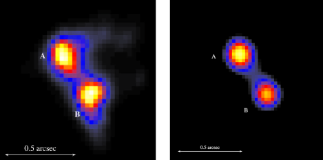
Figure 1.— Deconvolved image (left panel) of the 2002 February 24 Chandra  observation of APM 08279+5255. North is up, and east is to the left. Best fit PSF model (right panel) to the same observation of APM 08279+5255.

2.1. Properties of the fast outflow of APM 08279+5255

APM 08279+5255 is a gravitationally lensed BAL quasar at redshift z=3.911 (Downes et al., 1999). Its bolometric luminosity estimated as $L_{\rm bol}=7\times 10^{15}\mu_{L}^{-1}L_{\odot}$ ($\mu_{L}$ is the lens amplification factor; Irwin et al., 1998; Riechers et al., 2009) makes this source one of the most luminous in the universe, despite the value of the lens amplification factor. The presence of high-ionization BAL features produced in C iv, O vi, N v and Ly $\alpha$ transitions indicates that it is a high ionization BAL quasar (HiBAL). The C iv BAL of APM 08279+5255 contains multiple absorption troughs with widths ranging between 2000 km s^-1 and 2500 km s^-1. The maximum observed outflow velocity of the C iv absorption is $v_{\rm max(CIV)}\sim 0.04c$ relative to the source systemic redshift of $z=3.911$ (Srianand & Petitjean, 2000).

Table 1Log of observations of APM 08279+5255.

Datea	OBS ID	Telescope	Instrument	Exposure	Net exp	Net countsb	$f_{0.5-8}$c
2002-02-24 (Epoch1)	2979	Chandra	ACIS BI	91.9 ks	88.8 ks	5,627$\pm$75	5.44$\pm$0.15
2002-04-28 (Epoch2)	0092800201	XMM-Newton	EPIC pn	102.9 ks	83.5 ks	12,820$\pm$139	5.51$\pm$0.15
2006-10-12 (OBS1)	701057010	Suzaku	XIS FI	102.3 ks	71.3 ks	6,071$\pm$90	5.58$\pm$0.34
2006-10-12 (OBS1)	701057010	Suzaku	XIS BI	102.3 ks	71.3 ks	2,325$\pm$64	5.39$\pm$0.43
2006-11-01 (OBS2)	701057020	Suzaku	XIS FI	102.3 ks	67.9 ks	5498$\pm$87	5.18$\pm$0.32
2006-11-01 (OBS2)	701057020	Suzaku	XIS BI	102.3 ks	67.9 ks	2,181$\pm$62	5.15$\pm$0.37
2007-03-24 (OBS3)	701057030	Suzaku	XIS FI	117.1 ks	86.4 ks	4750$\pm$80	5.55$\pm$0.49
2007-03-24 (OBS3)	701057030	Suzaku	XIS BI	117.1 ks	86.4 ks	2,918$\pm$71	5.63$\pm$0.39
2007-10-06 (Epoch3)	0502220201	XMM-Newton	EPIC pn	89.6 ks	56.4 ks	11,400$\pm$114	6.04$\pm$0.16
2007-10-22 (Epoch4)	0502220301	XMM-Newton	EPIC pn	90.5 ks	60.4 ks	16,698$\pm$133	8.06$\pm$0.15
2008-01-14 (Epoch5)	7684	Chandra	ACIS BI	91.7 ks	88.06 ks	6,938$\pm$83	5.89$\pm$0.21

Gravitational lensing of APM 08279+5255 produces three images with the two brightest ones separated by $\sim$ 0.5″ (see Figure 1). The time-delay between images A and B of APM 08279+5255 is estimated to be of the order of a few hours (e.g., Muñoz, Kochanek & Keeton, 2001). The Eddington ratio of APM 08279+5255 can be estimated from an assumed value of $\Gamma\sim 2$ (where $\Gamma$ is the X-ray photon index), which is close to the mean value estimated from observations (Saez, Chartas & Brandt, 2009; Chartas et al., 2009a), and using the $L_{\rm bol}/L_{\rm Edd}$ vs. $\Gamma$ correlation found in RQ quasars (e.g., Wang et al., 2004; Shemmer et al., 2006, 2008). The $L_{\rm bol}/L_{\rm Edd}$ vs. $\Gamma$ correlation for APM 08279+5255 implies $L_{\rm bol}/L_{\rm Edd}\sim 0.2$, and therefore $M_{\rm BH}\sim 10^{12}\mu_{L}^{-1}M_{\odot}$. A second independent method of estimating the Eddington ratio through the use of the observed width of the C iv line indicates a black-hole mass of $M_{\rm BH}\sim 10^{11}\mu_{L}^{-1}M_{\odot}$ (see e.g., Riechers et al., 2009). The Eddington ratio derived using the second method is $L_{\rm bol}/L_{\rm Edd}\sim 2$, implying the source is accreting at a super-Eddington rate. However caution must be taken with this result because the estimates of $M_{\rm BH}$ based on C iv emission-line widths is subject to a lot of systematic uncertainties (i.e., it contains non-virial components such as the disk wind that can contribute to the broadening, e.g., Shemmer et al., 2008). There are also conflicting reported estimates of the magnification parameter ($\mu_{L}$). Optical observations indicate $\mu_{L}\sim 100$ (e.g, Egami al., 2000), while observations of CO emission yield $\mu_{L}\sim 4$ (e.g., Riechers et al., 2009). In this work we try, as far as possible, to present our results as a function of the magnification factor, however when this is not possible a value of $\mu_{L}=100$ is assumed (as in, Egami al., 2000). The absorption corrected optical to X-ray power-law slope, of APM 08279+5255  is $\hbox{$\alpha_{\rm ox}$}\sim-1.8$ (e.g., Dai et al., 2004). The relatively soft SED of APM 08279+5255 combined with its nearly large Eddington ratio provide ideal conditions for the production of radiatively driven winds (see e.g., Everett, 2005, and §4).

2.2. Results from eight deep X-ray observations of APM 08279+5255

This section summarizes results from 2 Chandra, 3 XMM-Newton and 3 Suzaku observations of APM 08279+5255 (8 in total; see Table 1 for details). The data reduction of the Chandra and XMM-Newton observations is described in Chartas et al. (2009a) and the reduction of the Suzaku  observations in Saez, Chartas & Brandt (2009). Note that from here on when we refer to a particular observation we will use the same names defined in Saez, Chartas & Brandt (2009) and Chartas et al. (2009a). Therefore the three Suzaku observations are referred to as OBS1, OBS2 and OBS3, the three XMM-Newton observations are referred to as Epoch 2, Epoch 3 and Epoch 4 and the two Chandra observations are referred to as Epoch 1 and Epoch 5 (see Table 1 for details).

Table 2 The minimum and maximum energies and velocities of the high-energy absorption features in APM 08279+5255^a.

OBS	Instrument		$E_{\rm min}$	$E_{\rm max}$	$v_{\rm min}$	$v_{\rm max}$	$\Gamma$
			[keV]	[keV]	[$c$]	[$c$]
OBS1	XIS FI		7.52$\pm$0.36	12.16$\pm$0.52	0.11$\pm$0.05	0.53$\pm$0.03	1.94$\pm$0.04
OBS2	XIS FI		7.88$\pm$0.48	11.57$\pm$0.51	0.16$\pm$0.06	0.50$\pm$0.03	2.02$\pm$0.03
OBS3	XIS FI		7.51$\pm$0.32	11.70$\pm$1.06	0.11$\pm$0.04	0.51$\pm$0.07	1.94$\pm$0.05
OBS1	XIS BI		7.24$\pm$0.51	12.47$\pm$1.12	0.08$\pm$0.07	0.55$\pm$0.06	1.95$\pm$0.07
OBS2	XIS BI		8.74$\pm$0.58	12.24$\pm$1.16	0.26$\pm$0.06	0.54$\pm$0.07	1.91$\pm$0.06
OBS3	XIS BI		7.53$\pm$0.82	12.40$\pm$0.92	0.12$\pm$0.11	0.54$\pm$0.05	1.92$\pm$0.05
Epoch1	ACIS S3		8.05$\pm$0.11	10.64$\pm$0.19	0.18$\pm$0.01	0.43$\pm$0.01	1.74$\pm$0.03
Epoch2	EPIC pn		7.54$\pm$0.42	15.04$\pm$0.97	0.12$\pm$0.06	0.67$\pm$0.04	1.89$\pm$0.03
Epoch3	EPIC pn		6.42$\pm$0.48	17.94$\pm$1.81	$<0.03$	0.76$\pm$0.04	2.03$\pm$0.04
Epoch4	EPIC pn		6.94$\pm$0.20	16.31$\pm$0.90	0.04$\pm$0.03	0.71$\pm$0.03	2.11$\pm$0.02
Epoch5	ACIS S3		7.36$\pm$0.30	15.35$\pm$1.13	0.09$\pm$0.04	0.68$\pm$0.04	1.94$\pm$0.04

Our analysis of the X-ray observations of the BAL quasar APM 08279+5255 indicates strong and broad absorption at rest-frame energies of 1–4 keV (low-energy) and 7–18 keV (high-energy). The medium producing the low-energy absorption is a nearly neutral absorber with a column density of $\hbox{log~{}($N_{\rm H}/{\rm cm}^{-2})$}\sim 23$. However, since APM 08279+5255 is at a high redshift of $z=3.91$ it is difficult to constrain the ionization state of the low-energy absorber. The absorption signatures of this complex low energy absorber are shifted outside the range of the observed X-ray band (typically between 0.3–10 keV). The high-energy absorption features are easily detected in the 8 deep X-ray observations of APM 08279+5255. In every case these features satisfy $\rm EW/\sigma_{EW}\gtrsim 3$ (see, Saez, Chartas & Brandt, 2009; Chartas et al., 2009a), and therefore they satisfy realistic limits for significant detections (Vaughan & Uttley, 2008).

Chartas el al. 2002 have interpreted the high-energy X-ray BALs as being produced by absorption of highly ionized iron such as Fe xxv  K$\alpha$ ($1s^{2}-1s2p$; 6.70 keV) and/or Fe xxvi  ($1s-2p$; 6.97 keV) launched very near an ionizing compact central source. Evidence to support this interpretation is the significant variability in the strength and energy of the X-ray BALs over short time-scales present in many of the observations. This variability is found to be as short as $\sim$ 3 days rest-frame  in the Chandra and XMM-Newton observations, and $\sim$ month in the Suzaku observations. This fast variability presents a strong argument in favor of a wind that originates from a distance of a few times the Schwarzschild radius.

In the Suzaku observations the variability of the high energy absorber is present at energies close to 7 keV rest-frame. On the other hand the Chandra and XMM-Newton observations show variability of the high-energy absorption profiles at both: low energies (i.e. rest-frame energies $\sim 7$ keV) and high energies (i.e. rest-frame energies $\gtrsim 9$ keV). A time-variable outflow provides a plausible explanation for the changes in shape on the absorption features in past X-ray observations of APM 08279+5255 (Chartas et al., 2002; Hasinger et al., 2002). An even stronger case is presented in Chartas et al. (2009a) and Saez, Chartas & Brandt (2009), where it can be seen clearly that in some cases the appearance of the high-energy absorption feature can take the shape of a notch, an edge or two absorption lines. Our spectral analysis of the 8 deep observations also indicates variability of the parameters defining the high energy attenuation which is likely due to a change in the outflow velocity of the absorber (Saez, Chartas & Brandt, 2009; Chartas et al., 2009a). The short time-scale ($\sim$week in the rest-frame) of the variability combined with the high ionization of the absorbing material which is moving at relativistic speeds imply that the absorbers are launched from distances $\lesssim 10~{}R_{S}$ from the central source (see e.g §4 of Saez, Chartas & Brandt, 2009). The short time-scale of this variability in the Suzaku (Saez, Chartas & Brandt, 2009) and XMM-Newton (Chartas et al., 2009a) observations also indicates that this absorber should be strongly accelerated. The global covering factor of these winds should be low $\lesssim 20\%$ based on the absence of emission features from the outflowing ionized gas (see e.g. Chartas et al., 2009a).

The minimum and maximum projected velocities ($v_{\rm min},v_{\rm max}$) of the outflow are estimated from the minimum and maximum energy ranges ($E_{\rm min},E_{\rm max}$) of the high-energy absorption features in APM 08279+5255. We obtained $E_{\rm min}$ and $E_{\rm max}$ from our spectral fits assuming first the two absorption-line (APL+2AL) model. Specifically, based on the best-fit values of an absorbed power-law model with two absorption lines (from Table 3 of Saez, Chartas & Brandt 2009 and Table 2 of Chartas et al. 2009), we obtain $E_{\rm min}=E_{\rm abs1}-2\sigma_{\rm abs1}$ and $E_{\rm max}=E_{\rm abs2}+2\sigma_{\rm abs2}$. As in Chartas et al. (2009a), we estimate the line of sight projected velocities $v_{\rm min}$ and $v_{\rm max}$ assuming the absorption arises from highly blueshifted Fe xxv K$\alpha$ ($E_{\rm lab}=6.7$ keV). In Table 2 we show the values obtained for $E_{\rm min}$, $E_{\rm max}$, $v_{\rm min}$ and $v_{\rm max}$. In this table we also add a column with the fitted values of $\Gamma$ (based on the APL+2AL model). Using $E_{\rm max}$ $\sim$ 18 keV (the maximum observed value), we constrain the maximum angle between our line of sight and the wind direction to be less than $22^{\circ}$.

As we indicated in Chartas et al. (2009a) (and from Table 2) there is a hint that changes in the photon index ($\Gamma$) may be positively correlated with the changes of the maximum velocity of the outflow ($v_{\rm max}$). This possible trend between $\Gamma$ versus $v_{\rm max}$ is shown in Figure 10 of Chartas et al. (2009a). In §3 we recalculate the velocities found in Table 2 with a model based on cloudy simulations of a near-relativistic outflow. In §4 we provide an interpretation of the possible trend between maximum outflow velocity and $\Gamma$.

3. Photoionization models of near-relativistic outflows

3.1. Motivation

From the X-ray analysis of our 8 observations of APM 08279+5255 (see, Saez, Chartas & Brandt, 2009; Chartas et al., 2009a, for more details), and past observations of this object and PG 1115+080 (e.g., Chartas et al., 2007a), it became clear that a more sophisticated spectral model was needed to fit the X-ray BALs. Currently there are no proper tools available in the spectral fitting package xspec to model absorption profiles resulting from near-relativistic outflows. In Saez, Chartas & Brandt (2009) we used photoionization models created from the photoionization code xstar (see, e.g., Kallman & Bautista, 2001) to fit the broad absorption feature found between 7$-$18 keV rest-frame in APM 08279. This spectral analysis did not include relativistic corrections, and does not contain a realistic model of the outflow. In this section we describe new software code that we have developed that provides a more realistic description of radially accelerated near-relativistic outflows. Our main goal is to better constrain important parameters describing near-relativistic outflows; among these are, the velocity profile, the ionization parameter and the column density of the observed X-ray wind.

3.2. Description of the code

Our quasar outflow code is based on a multilayer approach which mimics the absorption and scattering through a near-relativistic outflow using the photoionization code cloudy (Ferland al., 1998). An existing quasar outflow code called xscort developed by Schurch & Done 2007 follows a similar approach and is based on the photoionization code xstar.

In our quasar outflow code we use cloudy simulations to approximate the absorption signature produced by an outflowing medium that is radiatively accelerated from a central source. We describe the outflowing medium with a set of absorption layers with specific velocity profile and ionization states. The details of the approximations and assumptions used in our quasar outflow model are described in the following paragraphs.

3.2.1 The case of one absorption layer

We approximate the attenuation through the outflowing ionized gas as the absorption through a series of layers of different velocities and ionization states. We begin by calculating the output absorption profile assuming the wind is made up of a single layer and then generalize our model by dividing the outflowing wind into multiple layers. We assume the layer is at a distance $R$ from the continuum source, has a thickness $\Delta R\ll R$, a density $n$, and is moving at a velocity $v$ away from it. We further assume that spectral energy distribution of the source is a power-law ($L_{\nu}\propto\nu^{\alpha}$) with spectral index $\alpha=-1.0$. From here on, unless mentioned otherwise, this is the SED that we will assume in our simulations. The ionization parameter (Tarter, Tucker & Salpeter, 1969, see Appendix A) measured in the absorption layer’s rest-frame is

$$\xi=\frac{4\pi F^{\prime}_{I}}{n^{\prime}}$$ (1)

where primed quantities $n^{\prime}$ ($n^{\prime}=\gamma n$) and $F^{\prime}_{I}$ refer to the density and the incident ionizing flux in the layer’s rest-frame, respectively. Non primed parameters are assumed to be in the rest-frame of the luminous source. Using the fact that $I_{\nu}/\nu^{3}$ is a Lorentz invariant, the incident ionization flux in a layer’s rest-frame is given by

$$F^{\prime}_{I}=\gamma^{4}(1-v/c)^{4}F_{I}.$$ (2)

The column density (in any reference frame) of the layer is given by $N_{\rm H}=n\Delta r$. The incident flux on a layer is calculated between 1–1000 Ry in the rest-frame of the moving layer. From the incident flux in the rest-frame of the layer and from the use of equation (1) we calculate the ionization state of this layer. We next input the derived ionization state and column density of the layer into the photoionization code cloudy  to obtain the output spectrum of the layer in its rest-frame and transform it to the rest-frame of the luminous source.

3.2.2 A model to describe X-ray absorption profiles.

The X-ray spectra that we have obtained from observations of several BAL quasars do not show any emission lines associated with the X-ray BALs (Chartas et al., 2009a). This is expected since BAL quasar outflows in general have relatively small global covering factors (Hewett & Foltz, 2003). Therefore, we will concentrate on absorption-dominated outflows neglecting emission features in our model. For our cloudy code, we will assume an approximately constant ionization parameter in the outflow.

We assume that the region of the outflow that contributes to the observed Fe xxv and/or Fe xxvi absorption is localized in a relatively thin multilayer of thickness $\Delta R$ at a distance $R$ from the black hole. The justification behind the assumption that $\Delta R\ll R$ in our model is that the presence of Fe xxv  is likely to occur in a relatively narrow region away from the source where the ionization parameter and density are such that Fe xxv  is abundant at these distances. Even though the ionization parameter is expected to fall off with distance along the flow as $1/R^{2}$ it remains relatively constant within the multilayer since $\Delta R\ll R$. To compensate for changes in flux across the multilayer due to relativistic effects (e.g., beaming effects) we adjust the density $n_{i}$ of each layer such that the ionization parameter remains approximately constant within the multilayer $\Delta R$. In the case that the region of the outflow that we are modeling is not physically thin, our approach will still be valid as long as the ionization parameter along this region does not change appreciably.

From equation (1) the ionization parameter of each layer is $\xi_{i}=4\pi F_{\rm I,i}^{\prime}/n^{\prime}_{i}$; where $F_{I,i}^{\prime}$ is the incident flux in the rest-frame of layer $i$ estimated from the flux coming from layer $i-1$ after taking into account relativistic effects. The density of each layer, is determined from an a priori defined velocity profile $v(r)$. In our multilayer approach, the density of each layer is $n_{i}\propto\gamma_{i}^{3}(1-v_{i}/c)^{4}$ for $i=0,1..(N_{l}-1)$, were $N_{l}$ is the number of layers. We note that the assumed density profile adjusts the ionization parameter so that it does not vary across the multilayer due to relativistic effects. However, the ionization parameter will still decrease between $0.02-0.40$ dex mainly due to attenuation (see §3.2.3). For our case we concentrate on simulated outflows with ${\rm log~{}}\xi\gtrsim 3$. As long as each layer used in our calculations has a column density of ${\rm log}~{}(\Delta\hbox{${N}_{\rm H}$}_{i}/{\rm cm}^{-2})\lesssim 23$ it can be assumed to be almost transparent (or thin) to radiation (see Appendix B). As we describe in §3.2.3 the assumption of optically thin layers will allow us to more greatly reduce the time needed to compute the absorption signature of the multilayered outflow.
In this work we assume that the outflow velocity profile will have a $p$-type form given by

$$v(\hat{N}_{\rm H})=v_{\rm min}+(v_{\rm max}-v_{\rm min})(\hat{N}_{\rm H}/\hbox{${N}_{\rm H}$})^{p},$$ (3)

where ${N}_{\rm H}$ is the total column density of the simulated wind ($0<\hat{N}_{\rm H}<\hbox{${N}_{\rm H}$}$). We note that given the assumptions described here, and the moderate S/N of the absorption profile in X-ray, we do not expect to obtain significant constraints on the acceleration mechanism of the outflow by using this profile.

3.2.3 Passing a continuum spectrum from one absorbing layer to the next

When passing the continuum spectrum from one layer ($i$-1) to the next ($i$) we first transform the source rest-frame spectrum coming from layer $i$-1 to the rest-frame of layer $i$. In the rest-frame of layer $i$ we remove absorption and add emission (in cases where we do consider emission) to the incident spectrum given the column density and ionization parameter of the layer. The column density of layer $i$ is obtained from the velocity profile, and its ionization parameter is calculated from the input spectrum in its rest-frame. Finally we transform the output spectrum coming from layer $i$ back to the source rest-frame.

Since the density of each layer is chosen to correct the attenuation of the flux due to relativistic effects, the ionization parameter will mostly decrease due to the absorption of the outflow across the layer. The decrease of the ionization through the multilayered outflow due to absorption will be greater in winds that are less ionized and with higher column densities. For example, a wind with $\hbox{log~{}($N_{\rm H}/{\rm cm}^{-2})$}=22.75$ with initial ionization parameter of $\hbox{log~{}$\xi$}_{i}=3.25$ will have a final ionization parameter of $\hbox{log~{}$\xi$}_{f}\sim 3.21$, however for $\hbox{log~{}($N_{\rm H}/{\rm cm}^{-2})$}=22.75$ and $\hbox{log~{}$\xi$}_{i}=3.75$ the final ionization parameter is $\hbox{log~{}$\xi$}_{f}\sim 3.73$. Additionally a wind with $\hbox{log~{}($N_{\rm H}/{\rm cm}^{-2})$}=23.75$ and $\hbox{log~{}$\xi$}_{i}=3.25$ will have $\hbox{log~{}$\xi$}_{f}\sim 2.84$, however if $\hbox{log~{}($N_{\rm H}/{\rm cm}^{-2})$}=23.75$ and $\hbox{log~{}$\xi$}_{i}=3.75$ then $\hbox{log~{}$\xi$}_{f}\sim 3.53$.

After correcting the spectrum incident on layer $i$ for the effects of relativistic beaming, we estimate the absorption and emission from layer $i$ using simulations performed with the photoionization code cloudy. These cloudy simulations are implemented using the unabsorbed source spectrum (power-law with $\alpha=-1$ in our case) and various values of the ionization parameter. The main advantage of this approximation is a dramatic shortening in the time it takes to obtain a profile. This speed-up is possible because the photoionization runs at each layer use a library of preexisting cloudy runs (see next paragraph for details). If the flux emitted by the source is a power-law, the flux received by a moving layer is also a power-law with the same spectral index as the source as long as the SED is not significantly attenuated in an energy dependent way. In addition, if each layer of the multilayered media is approximately optically thin then the state of the gas depends primarily on the ionization parameter and secondarily on the SED (Tarter, Tucker & Salpeter, 1969). This dependence indicates that our approach is at first order a good approximation as long as the SED along the multilayered outflow does not differ appreciably from the incident SED at the first layer. However, for low ionization states ($\hbox{log~{}$\xi$}<3$) and large total column densities ($\hbox{log~{}($N_{\rm H}/{\rm cm}^{-2})$}\gtrsim 23.5$), the SED along the multilayered outflow will deviate appreciably from the initial incident SED, and therefore, our approximation breaks down.

In order to avoid invoking cloudy too many times ($\sim 100$) to simulate the signature of the multilayered absorber, we created a library of spectra to speed-up our calculations. This library contains a set of simulated transmitted spectra through absorbers having a range of ionization parameters between $1.8-4.1$ dex (log $\xi$ steps of 0.01 dex), column density of $\hbox{log~{}($N_{\rm H}/{\rm cm}^{-2})$}=19$, density of $n_{\rm H}=10^{12}$ cm^-3 and an input SED that has the form of a power law ($L_{\nu}\propto\nu^{\alpha}$) in the energy range between $1-10^{4}$ Rys with spectral index $\alpha=-1$. The value of the density of the absorber ($n_{\rm H}=10^{12}$ cm^-3) is chosen to be close to the value of the density predicted by 2-d numerical simulations of radiative winds by Proga et al. (2000, 2004). The simulations used to construct this library (from here on referred to as library runs), as well as all the simulated profiles described in the next sections, are calculated using standard solar metallicities. We primarily used cloudy to perform the photoionization calculations but we also compared our results with those generated by the photoionization code xstar.

In order to reduce the number of realizations in our library, we performed these runs assuming a specific turbulent velocity of $v_{\rm turb}=1500~{}\hbox{km~{}s${}^{-1}$}$. Our choice of a specific turbulent velocity requires that the relative speed $\Delta v_{i}^{\prime}$ between layers $i$ and $i+1$ to be the same for every layer in the simulations of multilayered outflows (i.e. $\Delta v_{i}^{\prime}=\Delta v^{\prime}$; see Appendix C). In our simulations we use a finite number of layers to describe the outflow, each layer having a slightly different velocity following the adopted velocity profile. The distribution of the velocity differences between adjacent layers is assumed to be uniform and to extend between 0 and a maximum velocity difference of $\Delta v^{\prime}$. The velocity difference of $\Delta v^{\prime}$ is kept lower than $v_{\rm turb}\sqrt{12}$; where $v_{\rm turb}=1500~{}\hbox{km~{}s${}^{-1}$}$ is the assumed turbulent velocity (see Schurch & Done, 2007). By selecting a turbulent velocity we set a lower limit on the number of layers used in simulating a BAL spectrum. The simulations making up our library are all performed using the same column density ($\hbox{log~{}($N_{\rm H}/{\rm cm}^{-2})$}=19$). Consequently, the opacity of a layer $i$ (i.e., the layer’s rest-frame absorption) is calculated by first obtaining the opacity from the library at the ionization state of the layer, and second, by scaling the opacity obtained (from the library) to the column density of the layer. This approximation is justified given that in the range of densities of our simulations ($8\lesssim\rm log~{}\hbox{${n}_{\rm H}$}\lesssim 12$) the dependency of the opacity on $n_{H}$ is negligible, and therefore, the opacity of a layer $i$ can be found from the library just by knowing its ionization state and column density. Emission spectra may also be obtained from our library runs, however for our study we mostly concentrated on the absorption spectra. We focus on the absorption spectra since the main goal of our study is to fit the spectral signatures produced by winds in which emission lines are relatively weak implying low global covering factors. Additionally, we assume that the line-of-sight covering factor is equal to one.

3.2.4 Testing our relativistic outflow code

We first generate the absorption profiles for a linearly accelerated outflow with $v_{\rm min}=0$, $v_{\rm max}=0.3c$ ($v\propto\hbox{${N}_{\rm H}$}$), $\hbox{${N}_{\rm H}$}=3\times 10^{23}$ cm^-2, initial density $n_{0}=10^{12}$ cm^-3, and values of $\hbox{log~{}$\xi$}=$ 2.75, 3.00, 3.25, 3.50, 3.75 and 4.00. These profiles have been generated to compare the results of our code with those presented in Schurch & Done (2007). In order to make a fair comparison with the results of Schurch & Done (2007), we use a library of xstar runs using a power-law model with $\alpha=-1.4$. This library of xstar runs, has the same characteristics as the cloudy library described in §3.2.3. Our simulated X-ray absorption profiles are very similar to the ones computed by Schurch & Done 2007 under the assumption of a multilayer outflow with spherical symmetry (see Appendix D).

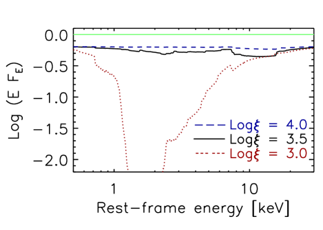
Figure 2.— X-ray spectra derived from multilayered cloudy simulations of near-relativistic outflows. The assumed input spectrum is a power-law with $\Gamma=2.0$. The outflow has been accelerated between $0.1c-0.7c$ using a $p$-type velocity profile with $p=1.0$. The total column density of the outflow is $\hbox{log~{}($N_{\rm H}/{\rm cm}^{-2})$}=23.75$. We have calculated the output spectra for 3 different values of the ionization parameter, log $\xi$ = 3.0, 3.5 and 4.0.

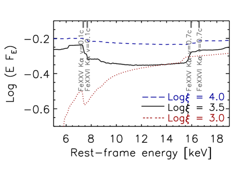
Figure 3.— X-ray spectra derived from multilayered cloudy simulations of near-relativistic outflows. This is a zooming of Figure 2 in the region where we find iron absorption. The assumed input spectrum is a power-law with $\Gamma=2.0$. The outflow has been accelerated between $0.1c-0.7c$ using a $p$-type velocity profile with $p$=1.0. The total column density of the outflow is $\hbox{log~{}($N_{\rm H}/{\rm cm}^{-2})$}=23.75$. We have calculated the output spectra for 3 different values of the ionization parameter, log $\xi$ = 3.0, 3.5 and 4.0. For reference the observed blueshifted energies of the Fe xxv K$\alpha$ and Fe xxvi K$\alpha$ lines with $v=0.1c$ and of the Fe xxv K$\alpha$ and Fe xxvi K$\alpha$ lines with $v=0.7c$ are highlighted.

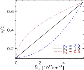
Figure 4.— Outflow velocity as a function of column density through the outflow for 3 different values of the the exponent of the $p$-type velocity profile (see equation 3), $p$ = 0.5 (dotted line), 1.0 (solid line) and 2.0 (dashed line). We assumed the outflow has a launch velocity of 0.1 $c$, a terminal velocity of 0.7 $c$ and a total column density of $\hbox{log~{}($N_{\rm H}/{\rm cm}^{-2})$}=23.75$.

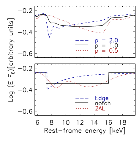
Figure 5.— Upper panel: X-ray spectra produced from multilayered cloudy simulations of near-relativistic outflows. The assumed input spectrum is a power-law with $\Gamma=2.0$ (solid line). The outflow has been accelerated between 0.1$c$$-$0.7$c$ using an exponent of the velocity profile with $p$=1.0. The total column density of the outflow is $\hbox{log~{}($N_{\rm H}/{\rm cm}^{-2})$}=23.75$. We have calculated the output spectra for 3 different values of the exponent $p$, $p$ = 0.5 (dotted line), 1.0 (solid line) and 2.0 (dashed line). Lower panel: X-ray spectra resulting from the best fitted models used in Chartas et al. (2009a) to fit the high energy absorption of APM 08279+5255  in Epoch 3. The solid line is for the notch model, the dotted line corresponds to the two absorption line model and the dashed line is for the absorption edge model.

We generate a second run of simulations based on our results presented in §2.2. For this purpose, we simulate absorption profiles with $v_{\rm min}=0.1c$, $v_{\rm max}=0.7c$, $n_{0}=10^{12}~{}\hbox{cm${}^{-3}$}$, $\hbox{log~{}($N_{\rm H}/{\rm cm}^{-2})$}=23.75$, and three values of the ionization parameter $\hbox{log~{}$\xi$}=3.0,3.5,4.0$. The outflow parameters have been chosen approximately in accordance to the estimated values based on one of the XMM-Newton observations of APM 08279+5255  (Epoch 3 from Chartas et al., 2009a). To generate notch-type absorption profiles we chose $p=1$ for these simulations. The resulting profiles are presented in Figure 2. In Figure 3 we zoom in on the iron blend feature which shows up at energies between 7.5$-$16.5 keV. The resonance absorption lines responsible for the features are mainly Fe xxv  K$\alpha$ ($1s^{2}-1s2p$; 6.70 keV) and Fe xxvi  K$\alpha$ ($1s-2p$; 6.97 keV). From Figures 2 and 3 it is clear that the strength of the iron blend feature is larger for $\hbox{log~{}$\xi$}=3.5$. The strength of this feature is large for ionization parameters in the range of $3\lesssim\hbox{log~{}$\xi$}\lesssim 4$, since at lower ionization levels the abundance of highly ionized iron atoms (e.g., Fe xxv and Fe xxvi) is too small to produce any appreciable feature in the spectra. At $\hbox{log~{}$\xi$}\gtrsim 4$ the atoms in the gas become stripped of almost all their electrons, and therefore, the resulting spectra contain very few bound-bound and bound-free absorption features. When $\hbox{log~{}$\xi$}\lesssim 3$ there is substantial absorption present at rest-frame energies $\lesssim$ 2 keV. As a consequence, in a heavily absorbed source like APM 08279+5255, the low-energy ($\lesssim$ 2 keV) absorbed component of the spectrum, possibly due to non-outflowing material, will overlap with the absorbed component produced by the wind (e.g., Saez, Chartas & Brandt, 2009; Chartas et al., 2009a). However, the high-energy absorption iron trough (above $\sim 7$ keV) is not contaminated by absorption lines from non-outflowing material, and consequently, it provides a clean signature of the outflowing material.

The absorption profiles described in §2.2 contain a diversity of shapes, sometimes resembling notches, edges or two absorption lines. Given the variety of shapes of the absorption profiles we attempted to emulate these different shapes by generating simulations of outflows with $v_{\rm min}=0.1c$ and $v_{\rm max}=0.7c$, $\hbox{log~{}($N_{\rm H}/{\rm cm}^{-2})$}=23.75$, $\hbox{log~{}$\xi$}=3.5$ and three values of $p$, $p=0.5,1$ and 2. The output spectra of the resulting velocity profiles (see Figure 4 ) are presented in Figure 5. In the lower panel of Figure 5 we also show as a reference three model spectra used to fit Epoch 3. The three different models used are a notch, an edge and a two absorption line model (see Table 2 from Chartas et al., 2009a).

3.3. Fits to the observed spectra of APM 08279+5255 using our quasar outflow model

In this section we present results from fits to spectra obtained from XMM-Newton, Chandra and Suzaku observations of APM 08279+5255 using our thin multilayered outflow model. We created xspec table models from a large number of simulated quasar absorption spectra produced from running our multilayered model over a large range of parameter space of the outflow parameters. Specifically, the parameter space of our simulations covered five important properties of the multilayered outflow model: minimum velocity of the outflowing gas $v_{\rm min}$, maximum velocity $v_{\rm max}$, ionization parameter $\xi$, total column density ${N}_{\rm H}$ and the value $p$ which defines the outflow velocity profile (see equation 3). For our simulations we assume (unless mentioned otherwise) an initial density of the outflowing gas in the multilayer of $n_{0}=10^{12}$ cm^-3. We note that our results are not sensitive to the assumed initial density of the outflowing gas. A change of the density by up to two orders of magnitudes from our assumed value does not result in any significant variation of our results.

3.3.1 xspec table models for quasar outflows

In order to fit the variety of absorption spectra of APM 08279+5255 we generated three different types of xspec table models that mainly differ in the parameter space of the outflow properties that are covered.

The first table model (windfull.tab) assumes the presence of only one outflowing component. We define as component $i$ of an outflow a multilayer absorber at a distance $R_{\rm i}$ from the black hole, with a thickness $\Delta R_{\rm i}$ ($\Delta R_{\rm i}/R_{\rm i}\ll 1$), a velocity gradient of $\Delta v_{i}$ across it, a column density of $N_{\rm H}$, and an ionization parameter of $\hbox{log~{}$\xi$}_{i}$. We produced the table model windfull.tab by simulating transmitted spectra through a range of outflows with minimum velocities ($v_{\rm min}$) in the range of 0.0$-$0.3$c$ (a simulation for every 0.02$c$ interval), with maximum velocities ($v_{\rm max}$) in the range of 0.3$-$0.9$c$ (step intervals of 0.04$c$), log ($N_{\rm H}/{\rm cm}^{-2})$ in the range 22$-$24 (step intervals of 0.25 dex), log $\xi$ in the range 2.8$-$4.0 (step intervals of 0.2 dex), and the index $p$ having values of 0.5, 1.0, 2.0 and 5.0.

Table 3 Results from spectral fits to the three Suzaku observations of APM 08279+5255.

		FI   SPECTRUMb				BI   SPECTRUMb
		$\overline{\hskip 150.0pt}$				$\overline{\hskip 150.0pt}$
Modela	Parameter	Values OBS1	Values OBS2	Values OBS3		Values OBS1	Values OBS2	Values OBS3
MODEL1..	$\Gamma$	$1.96_{-0.05}^{+0.04}$	$2.03_{-0.05}^{+0.06}$	$1.95_{-0.06}^{+0.06}$		$2.03_{-0.15}^{+0.15}$	$1.93_{-0.05}^{+0.07}$	$1.91_{-0.07}^{+0.09}$
	${\rm log}~{}(N_{\rm H1}/{\rm cm}^{-2})$	$22.91_{-0.05}^{+0.09}$	$22.95_{-0.12}^{+0.12}$	$22.83_{-0.09}^{+0.11}$		$22.76_{-0.13}^{+0.12}$	$22.79_{-0.09}^{+0.06}$	$22.78_{-0.09}^{+0.08}$
	${\rm log}~{}(N_{\rm H2}/{\rm cm}^{-2})$	$23.54_{-0.11}^{+0.10}$	$23.32_{-0.15}^{+0.18}$	$23.55_{-0.15}^{+0.12}$		$23.82_{-0.16}^{+0.18}$	$23.42_{-0.15}^{+0.16}$	$23.68_{-0.22}^{+0.20}$
	$\hbox{log~{}$\xi$}_{2}$	$3.44_{-0.24}^{+0.16}$	$3.29_{-0.10}^{+0.10}$	$3.52_{-0.12}^{+0.16}$		$3.59_{-0.17}^{+0.25}$	$3.52_{-0.25}^{+0.12}$	$3.64_{-0.27}^{+0.22}$
	$v_{\rm min}/c$	$0.14_{-0.02}^{+0.02}$	$0.19_{-0.02}^{+0.02}$	$0.10_{-0.02}^{+0.02}$		$0.07_{-0.06}^{+0.03}$	$0.28_{-0.07}^{+0.04}$	$0.13_{-0.06}^{+0.03}$
	$v_{\rm max}/c$	$0.50_{-0.02}^{+0.04}$	$0.51_{-0.04}^{+0.04}$	$0.49_{-0.08}^{+0.12}$		$0.58_{-0.05}^{+0.05}$	$0.60_{-0.07}^{+0.06}$	$0.62_{-0.10}^{+0.15}$
	$p$	$1.6_{-0.4}^{+0.4}$	$1.8_{-0.6}^{+0.8}$	$2.3_{-0.7}^{+1.0}$		$1.4_{-0.6}^{+0.6}$	$2.8_{-1.0}^{+2.2}$	$2.6_{-1.4}^{+2.0}$
	log $L_{2-10}$	46.92$\pm$0.08	46.91$\pm$0.07	46.93$\pm$0.08		47.10$\pm$0.16	46.85$\pm$0.08	46.95$\pm$0.10
	$\chi^{2}/\nu$	60.5/67	68.8/60	70.2/65		56.1/65	89.6/60	43.8/65
	$P(\chi^{2}/\nu)$	0.70	0.21	0.32		0.78	0.01	0.98
MODEL2..	$\Gamma$	$1.98_{-0.05}^{+0.05}$	$2.03_{-0.04}^{+0.04}$	$1.95_{-0.05}^{+0.05}$		$2.00_{-0.10}^{+0.10}$	$1.92_{-0.05}^{+0.05}$	$1.91_{-0.07}^{+0.07}$
	${\rm log}~{}(N_{\rm H1}/{\rm cm}^{-2})$	$22.82_{-0.20}^{+0.16}$	$22.97_{-0.07}^{+0.07}$	$22.81_{-0.11}^{+0.13}$		$22.76_{-0.15}^{+0.10}$	$22.79_{-0.09}^{+0.09}$	$22.78_{-0.08}^{+0.06}$
	${\rm log}~{}(N_{\rm H21}/{\rm cm}^{-2})$	$23.23_{-0.15}^{+0.15}$	$23.10_{-0.14}^{+0.20}$	$23.08_{-0.20}^{+0.18}$		$23.50_{-0.18}^{+0.15}$	$23.42_{-0.22}^{+0.20}$	$23.48_{-0.32}^{+0.20}$
	${\rm log}~{}(N_{\rm H22}/{\rm cm}^{-2})$	$23.26_{-0.18}^{+0.20}$	$22.98_{-0.22}^{+0.26}$	$23.27_{-0.20}^{+0.28}$		$23.53_{-0.17}^{+0.16}$	$<23.5$	$23.40_{-0.36}^{+0.20}$
	$\hbox{log~{}$\xi$}_{2}$	$3.28_{-0.18}^{+0.28}$	$3.33_{-0.16}^{+0.12}$	$3.48_{-0.26}^{+0.20}$		$3.42_{-0.17}^{+0.16}$	$3.46_{-0.13}^{+0.14}$	$3.52_{-0.30}^{+0.25}$
	$v_{\rm min}^{(1)}/c$	$0.12_{-0.02}^{+0.02}$	$0.20_{-0.03}^{+0.03}$	$0.12_{-0.01}^{+0.01}$		$0.08_{-0.03}^{+0.02}$	$0.25_{-0.02}^{+0.02}$	$0.11_{-0.03}^{+0.04}$
	$v_{\rm max}^{(1)}/c$	$0.28_{-0.03}^{+0.03}$	$0.29_{-0.04}^{+0.04}$	$0.15_{-0.02}^{+0.02}$		$0.30_{-0.05}^{+0.05}$	$0.35_{-0.02}^{+0.02}$	$0.26_{-0.08}^{+0.08}$
	$v_{\rm min}^{(2)}/c$	$0.39_{-0.06}^{+0.06}$	$0.41_{-0.05}^{+0.05}$	$0.23_{-0.06}^{+0.06}$		$0.36_{-0.04}^{+0.04}$	$0.48_{-0.05}^{+0.05}$	$0.39_{-0.08}^{+0.08}$
	$v_{\rm max}^{(2)}/c$	$0.49_{-0.02}^{+0.03}$	$0.50_{-0.02}^{+0.02}$	$0.48_{-0.05}^{+0.05}$		$0.54_{-0.03}^{+0.03}$	$0.58_{-0.06}^{+0.04}$	$0.58_{-0.07}^{+0.07}$
	log $L_{2-10}$	46.95$\pm$0.08	46.92$\pm$0.07	46.91$\pm$0.08		47.08$\pm$0.09	46.87$\pm$0.07	46.98$\pm$0.12
	$\chi^{2}/\nu$	55.1/65	65.5/58	67.4/63		52.8/63	83.8/58	41.3/63
	$P(\chi^{2}/\nu)$	0.81	0.23	0.33		0.82	0.15	0.98

Table 4 Results from spectral fits of the Chandra and XMM-Newton observations of APM 08279+5255.

Modela	Parameter	Values Epoch 1	Values Epoch 2	Values Epoch 3	Values Epoch 4	Values Epoch 5
MODEL1…	$\Gamma$	$1.75_{-0.03}^{+0.04}$	$2.00_{-0.05}^{+0.06}$	$2.13_{-0.05}^{+0.09}$	$2.38_{-0.08}^{+0.09}$	$1.96_{-0.03}^{+0.03}$
	${\rm log}~{}(N_{\rm H1}/{\rm cm}^{-2})$	$22.67_{-0.07}^{+0.04}$	$22.72_{-0.07}^{+0.04}$	$22.71_{-0.02}^{+0.02}$	$22.68_{-0.02}^{+0.02}$	$23.02_{-0.03}^{+0.03}$
	${\rm log}~{}(N_{\rm H2}/{\rm cm}^{-2})$	$23.62_{-0.06}^{+0.05}$	$23.67_{-0.06}^{+0.06}$	$23.76_{-0.05}^{+0.08}$	$23.85_{-0.05}^{+0.06}$	$23.13_{-0.11}^{+0.09}$
	$\hbox{log~{}$\xi$}_{2}$	$3.56_{-0.12}^{+0.08}$	$3.35_{-0.10}^{+0.09}$	$3.47_{-0.10}^{+0.10}$	$3.36_{-0.05}^{+0.05}$	$3.28_{-0.10}^{+0.12}$
	$v_{\rm min}/c$	$0.15_{-0.01}^{+0.01}$	$0.13_{-0.01}^{+0.01}$	$0.08_{-0.02}^{+0.02}$	$0.05_{-0.01}^{+0.01}$	$0.13_{-0.03}^{+0.03}$
	$v_{\rm max}/c$	$0.43_{-0.04}^{+0.03}$	$0.64_{-0.06}^{+0.07}$	$0.69_{-0.03}^{+0.03}$	$0.73_{-0.02}^{+0.03}$	$0.31_{-0.02}^{+0.02}$
	$p$	$3.8_{-1.0}^{+1.0}$	$2.2_{-0.5}^{+0.8}$	$1.6_{-0.2}^{+0.2}$	$1.5_{-0.1}^{+0.2}$	$1.2_{-0.4}^{+0.6}$
	log $L_{2-10}$	46.83$\pm$0.06	47.01$\pm$0.07	47.15$\pm$0.08	47.48$\pm$0.12	46.91$\pm$0.04
	$\chi^{2}/\nu$	132.1/104	110.5/115	109.4/105	152.4/143	77.2/70
	$P(\chi^{2}/\nu)$	0.03	0.60	0.36	0.28	0.26
MODEL2…	$\Gamma$	$1.77_{-0.02}^{+0.02}$	$2.04_{-0.05}^{+0.05}$	$2.17_{-0.07}^{+0.06}$	$2.31_{-0.05}^{+0.08}$	$1.99_{-0.04}^{+0.05}$
	${\rm log}~{}(N_{\rm H1}/{\rm cm}^{-2})$	$22.61_{-0.05}^{+0.05}$	$22.63_{-0.05}^{+0.05}$	$22.67_{-0.05}^{+0.04}$	$22.63_{-0.03}^{+0.03}$	$23.01_{-0.04}^{+0.04}$
	${\rm log}~{}(N_{\rm H21}/{\rm cm}^{-2})$	$23.27_{-0.08}^{+0.11}$	$23.17_{-0.13}^{+0.12}$	$23.60_{-0.08}^{+0.07}$	$23.34_{-0.10}^{+0.06}$	$23.22_{-0.10}^{+0.08}$
	${\rm log}~{}(N_{\rm H22}/{\rm cm}^{-2})$	$23.08_{-0.12}^{+0.12}$	$23.47_{-0.13}^{+0.10}$	$23.41_{-0.12}^{+0.12}$	$23.51_{-0.07}^{+0.07}$	$23.12_{-0.22}^{+0.13}$
	$\hbox{log~{}$\xi$}_{2}$	$3.32_{-0.19}^{+0.18}$	$3.22_{-0.06}^{+0.06}$	$3.37_{-0.08}^{+0.08}$	$3.28_{-0.04}^{+0.04}$	$3.25_{-0.11}^{+0.15}$
	$v_{\rm min}^{(1)}/c$	$0.15_{-0.01}^{+0.01}$	$0.13_{-0.02}^{+0.02}$	$0.04_{-0.02}^{+0.02}$	$0.06_{-0.03}^{+0.02}$	$0.11_{-0.01}^{+0.01}$
	$v_{\rm max}^{(1)}/c$	$0.17_{-0.01}^{+0.01}$	$0.31_{-0.04}^{+0.04}$	$0.40_{-0.05}^{+0.05}$	$0.21_{-0.05}^{+0.05}$	$0.31_{-0.02}^{+0.02}$
	$v_{\rm min}^{(2)}/c$	$0.32_{-0.02}^{+0.02}$	$<0.12$	$0.43_{-0.10}^{+0.10}$	$0.24_{-0.06}^{+0.06}$	$0.58_{-0.04}^{+0.04}$
	$v_{\rm max}^{(2)}/c$	$0.40_{-0.01}^{+0.01}$	$0.63_{-0.03}^{+0.04}$	$0.69_{-0.03}^{+0.03}$	$0.73_{-0.02}^{+0.02}$	$0.66_{-0.03}^{+0.02}$
	log $L_{2-10}$	46.79$\pm$0.05	47.03$\pm$0.06	47.18$\pm$0.08	47.40$\pm$0.07	46.98$\pm$0.06
	$\chi^{2}/\nu$	116.8/102	107.5/113	106.5/103	152.5/141	66.2/68
	$P(\chi^{2}/\nu)$	0.15	0.63	0.39	0.24	0.54

In several observations, the X-ray BALs produced by highly ionized iron lines (above 7 keV rest-frame) appear to consist of two broad absorption components. The component covering low energies ($\lesssim$ 9 keV rest-frame) is referred to as slow and the one covering larger energies ($\gtrsim$ 10 keV rest-frame) is referred to as fast. Typical models used to fit the fast component contain a number of gaussian lines (Chartas et al., 2002, 2007a, 2009a; Saez, Chartas & Brandt, 2009). We created the table model windvslow.tab to fit the slow component and the table model windvfast.tab to fit the fast component. Since table models windvslow.tab and windvfast.tab are used to fit a relative small portion of the spectra we fix the velocity profile parameter to $p=1.0$. Each component of the outflow has a velocity gradient ${\Delta v}$ with a minimum ($v_{\rm min}$) and maximum velocity ($v_{\rm max}$) that satisfy $v_{\rm max}=v_{\rm min}+\Delta v$. By fitting these table models to the spectra we constrain the minimum and maximum projected velocities of each component. Table model windvslow.tab is generated with $\Delta v$ having values in the range 0.02-0.42$c$ (step intervals of 0.04$c$) and the parameters ($v_{\rm min}$), log $N_{\rm H}$ and log $\xi$ cover the same range and values as those used for producing table model windfull.tab. Table model windvfast.tab is generated with $\Delta v$ having values in the range 0.04-0.80$c$ (step intervals of 0.04$c$ for $\Delta v<0.24c$ and step intervals of 0.08$c$ for $\Delta v\geq 0.24c$) and the parameters $v_{\rm max}$, log $N_{\rm H}$ and log $\xi$ cover the same range and values as those used for producing table model windfull.tab.

3.3.2 Results from fits to X-ray spectra of APM 08279+5255

We fit the X-ray spectra of APM 08279+5255 using two different models. These two models assume a source spectrum consisting of a power-law attenuated by Galactic absorption (xspec model wabs). We assumed a Galactic column density of $4.1\times 10^{20}\hbox{cm${}^{-2}$}$ (Kalberla et al., 2005). The first model (MODEL1) contains an intrinsic neutral absorber (xspec model zwabs) to describe the absorption in the low energy range of 1$-$4 keV rest-frame and an outflowing ionized absorber (xspec table model windfull.tab) to account for the X-ray BALs. In xspec notation MODEL1 is written as:
wabs*zwabs*mtable{windfull.tab}*pow. The second model (MODEL2) contains an intrinsic neutral absorber (xspec model zwabs) to describe the absorption in the low energy range of 1$-$4 keV rest-frame and a two component outflowing ionized absorber (xspec table models windvslow.tab and windvfast.tab) to account for the X-ray BALs. In xspec notation MODEL1 is written as:
wabs*zwabs*mtable{windvslow.tab}*
mtable{windvfast.tab}*pow.

We note that MODEL1 and MODEL2 use a neutral absorber to describe the intrinsic attenuation in the low energy range of 1$-$4 keV rest-frame. In this work we also tried fits with an ionized absorber to describe the attenuation at 1$-$4 keV; these fits did not result in a significant improvement over fits that used a neutral absorber. Additionally, as discussed in Saez, Chartas & Brandt (2009); Chartas et al. (2009a), the use of a neutral absorber to describe the absorption in the low energy range of 1$-$4 keV rest-frame  did not improve with the use of more complex absorbers even for spectral fits performed to deep X-ray observations of APM 08279+5255. We also note that given the high redshift of APM 08279+5255, our fits to the spectra of this source cannot adequately constrain the low-energy intrinsic absorption at 1$-$4 keV rest-frame.
For MODEL2 the current data cannot adequately constrain the ionization parameters of both the slow and fast components of the outflow. We therefore set the ionization parameters of the slow and fast component to be equal in MODEL2.

Table 5 Estimates of the improvement of fits to the spectra of APM 08279+5255 using MODEL2 over MODEL1.

OBSID	Instrument	$F$-statistica	null probability	significance
OBS1	FI	2.59	4.8 $\times$ 10-2	95.2%
OBS1	BI	3.05	1.5 $\times$ 10-1	85.5%
OBS2	FI	5.32	2.4 $\times$ 10-1	76.0%
OBS2	BI	7.15	1.4 $\times$ 10-1	85.6%
OBS3	FI	1.31	2.8 $\times$ 10-1	72.3%
OBS3	BI	1.91	1.6 $\times$ 10-1	84.3%
Epoch 1	ACIS S3	6.68	1.8 $\times$ 10-3	99.8%
Epoch 2	EPIC pn	1.56	2.2 $\times$ 10-1	78.4 %
Epoch 3	EPIC pn	1.40	2.5 $\times$ 10-1	74.9 %
Epoch 4	EPIC pn	…	…	…
Epoch 5	ACIS S3	5.66	5.32 $\times$ 10-3	99.5%

The results of the fits of these models to the Suzaku spectra of APM 08279+5255 are presented in Table 3 and to the Chandra and XMM-Newton spectra in Table 4. We note that in MODEL1 of Tables 3 and 4 $\hbox{log~{}$N_{\rm H}$}_{1}$ and $\hbox{log~{}$N_{\rm H}$}_{2}$ are the best fitted column densities of the intrinsic neutral absorber and the outflowing ionized absorber, respectively. In MODEL2 of these same tables $\hbox{log~{}$N_{\rm H}$}_{1}$, $\hbox{log~{}$N_{\rm H}$}_{21}$, $\hbox{log~{}$N_{\rm H}$}_{22}$ are the best fitted column densities of the intrinsic neutral absorber, the slow and fast outflowing ionized absorber, respectively. In MODEL2 of these tables the velocity superscripts (1) and (2) represent the best-fitted velocity parameters of the slow and fast component, respectively.

In general the models that fit the high-energy outflowing absorber (see Tables 3 and 4) tend to have ionization parameters in the range $3.2\lesssim\hbox{log~{}$\xi$}\lesssim 3.7$. With the exception of the Chandra observations, there is no improvement in the fits when using MODEL2 over MODEL1. In Table 5 we show the statistical improvements based on the $F$-test of fits using MODEL2 over those using MODEL1. For the Chandra observations the improvements are $\gtrsim 99.5\%$ when we use MODEL2 over MODEL1. There are also marginal improvements using MODEL2 over MODEL1 for the Suzaku observations especially in OBS1 (see Table 5). In general we will use MODEL2 to estimate the outflow parameters because this model provides better constrains of the maximum velocity of the outflow. However, in the case of the XMM-Newton observations we use MODEL1 to estimate the outflow parameters because these observations show the widest X-ray BALs and provide better constraints of the velocity profile parameter $p$. We mainly used MODEL 1 to fit the XMM-Newton spectra of APM 08279+5255 because only one broad absorption trough is clearly observed at high energies. When we used Model 2 to fit the XMM-Newton spectra of APM 08279+5255 the two outflow components were found to overlap in velocity space. This overlap occurs when values of $v_{\rm max}^{(1)}$ are less or similar to $v_{\rm min}^{(2)}$, as presented in Table 4.

Based on the spectral fits to the Suzaku observations (Table 3), we find possible variability ($\gtrsim 2\sigma$) in the minimum velocity of the outflow between OBS2 and OBS3 ($v_{\rm min}$ in MODEL1 and $v_{\rm min}^{(1)}$ in MODEL 2) for both the BI and FI spectra. The evidence of this variability in the Suzaku spectra of APM 08279+5255  was already analyzed in Saez, Chartas & Brandt (2009) and in this work we conclude that its significance is at the 99.9% and 98% significance levels in the FI and BI spectra, respectively. This variability is also confirmed to exist between the column density and velocity of the slow component when we compare epochs OBS2 and OBS3.

We confirm the dramatic change in the maximum velocity of the fast component of the Chandra observations as shown in Chartas et al. (2009a). We find a $\gtrsim 3\sigma$ change of $v_{\rm max}^{(2)}$ between Epoch 1 and Epoch 5 using either MODEL1 or MODEL2 (see Table 4). We also confirm this change in velocity when we plot the confidence contours of the column density ($\hbox{log~{}$N_{\rm H}$}_{22}$) versus the maximum velocity of the fast outflow component ($v_{\rm max}^{(2)}$) using MODEL2. In Figure 6 we present confidence contours of $\hbox{log~{}$N_{\rm H}$}_{22}$ versus $v_{\rm max}^{(2)}$ for Epoch 1 and Epoch 5. The significance of the change of $\hbox{log~{}$N_{\rm H}$}_{22}$ versus $v_{\rm max}^{(2)}$ between Epochs 1 and 5 is $\gtrsim 99.9\%$ with a null probability of $\lesssim 10^{-4}$.

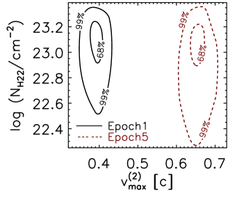
Figure 6.— Contour plots of the column density (${\rm log}~{}(N_{\rm H22}/{\rm cm}^{-2})$) versus maximum velocity ($v_{\rm max}^{(2)}$) of the fast component of the ionized outflow absorber. The contour plots have been calculated for the Chandra observations Epoch 1 (continuous line) and Epoch 5 (dashed line) at the 68% and 99% level of significance using MODEL2 of Table 4.

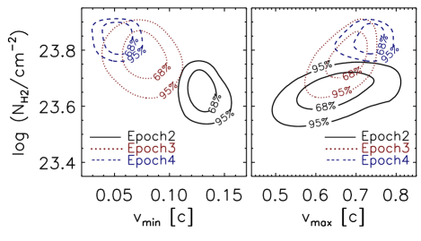
Figure 7.— Confidence contours of the total column density (${\rm log}~{}(N_{\rm H2}/{\rm cm}^{-2})$) versus minimum velocity ($v_{\rm min}$; left panel) and maximum velocity ($v_{\rm max}$; right panel) of the high-energy absorber. The contour plots have been calculated for the XMM-Newton observations Epoch 2 (solid line), Epoch 3 (dotted line) and Epoch 4 (dashed line) at the 68% and 95% level of significance using MODEL1 of Table 4.

Using either MODEL1 or MODEL2 we find a possible change in the maximum velocity of the outflow between the XMM-Newton observations of Epoch 2 and Epoch 4, however, the significance of this change is only at the 1$-$$\sigma$ level (see Table 4). We do find however significant changes in the minimum velocity and total column density of the outflow ($\hbox{log~{}$N_{\rm H}$}_{2}$; Table 4) between Epochs 2 and 4. In Table 4 we show that this variability is significant at the $\gtrsim$ 2$-$$\sigma$ level for fits using MODEL1. In Figure 7 we plot confidence contours of $\hbox{log~{}$N_{\rm H}$}_{2}$ versus $v_{\rm min}$ (left panel) and $\hbox{log~{}$N_{\rm H}$}_{2}$ versus $v_{\rm max}$ (right panel) for each XMM-Newton observation for fits using MODEL1. We find that the significance of the variability between Epoch 2 and Epoch 4 of $\hbox{log~{}$N_{\rm H}$}_{2}$ versus $v_{\rm min}$ is significant at the $\gtrsim 99.9\%$ level and of $\hbox{log~{}$N_{\rm H}$}_{2}$ versus $v_{\rm max}$ is significant at the $\gtrsim 99\%$ level. We also find variability in the minimum velocity of the outflow when we compare Epoch 2 and Epoch 3. This can be seen in Table 4 and the left panel of Figure 7. From the confidence contours (Figure 7, left panel), we estimate the significance of the variability on $\hbox{log~{}$N_{\rm H}$}_{2}$ versus $v_{\rm min}$ between Epoch 2 and Epoch 3 to be $\gtrsim 99\%$. It is worth mentioning that the fits using MODEL2 show an increase in the maximum velocity $\sim$ 2$-$$\sigma$ of the slow outflow component ($v_{\rm max}^{(1)}$) between Epoch 3 and Epoch 4. This change is consistent with the change found in the first component energy of the two gaussian absorption line model of Chartas et al. (2009a). Finally we note that the spectral fits to the XMM-Newton  observations show values of $p$ that are greater than one. Although we find indications of variability of $p$, these changes are not significant given the poor constraints of this parameter.

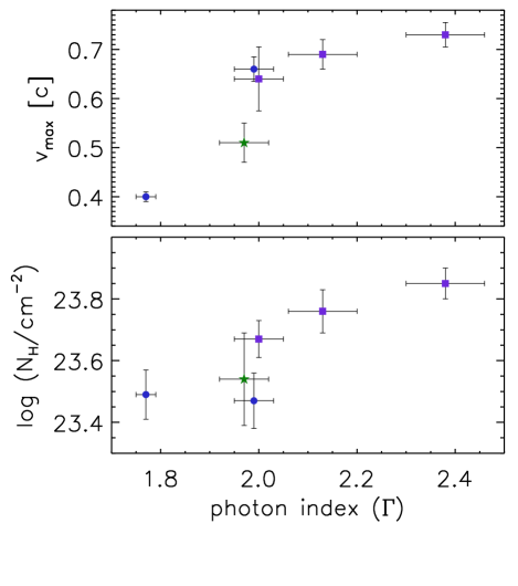
Figure 8.— Maximum velocity ($v_{\rm max}$; upper panel) and total column density of the outflow (log ($N_{\rm H}/{\rm cm}^{-2})$; lower panel) versus photon index ($\Gamma$) for our eight deep observations. $v_{\rm max}$, log ($N_{\rm H}/{\rm cm}^{-2})$ and $\Gamma$ were derived from fits to the spectra of APM 08279+5255 with a model that included an absorbed power-law and two component outflow (MODEL2 of Tables 3 and 4) for the Suzaku and Chandra observations and a single component outflow for the XMM-Newton observations (MODEL1 of Table 4). Errors shown are at the 68% confidence level. In each panel the Suzaku data points are displayed as a single point that represents the weighted (by total counts) mean of the three Suzaku observations. Data shown with circles, a star, and squares are obtained from Chandra, Suzaku and XMM-Newton observations respectively.

3.3.3 Mass outflow rate and kinetic energy of outflow of APM 08279+5255

We use results from fits of our quasar outflow model to the spectra of APM 08279+5255 to constrain the mass outflow rate and kinetic energy injected by this outflow into the surrounding medium. In Saez, Chartas & Brandt (2009) and Chartas et al. (2009a) we also constrained these properties of the outflow, however, these estimates were based on less realistic models (see §2.2).

Table 6 Mass-outflow rates and efficiencies of outflows in APM 08279+5255 ^a.

OBS	Instr.	$\dot{M}$ (abs1)	$\epsilon_{K}$ (abs1)	$\dot{M}$ (abs2)	$\epsilon_{K}$ (abs2)	$\dot{M}$ (tot)b	$\epsilon_{K}$ (tot)b
		[$10^{3}M_{\odot}\mu_{L}^{-1}{\rm yr}^{-1}$]		[$10^{3}M_{\odot}\mu_{L}^{-1}{\rm yr}^{-1}$]		[$10^{3}M_{\odot}\mu_{L}^{-1}{\rm yr}^{-1}$]
OBS1	XIS FI	$1.0^{+0.9}_{-0.6}$	$0.05^{+0.05}_{-0.03}$	$2.2^{+2.2}_{-1.5}$	$0.6^{+0.7}_{-0.4}$	$3.2^{+3.2}_{-2.1}$/$3.5^{+3.4}_{-2.3}$	$0.6^{+0.7}_{-0.4}$/$0.9^{+1.0}_{-0.6}$
OBS2	XIS FI	$0.9^{+0.8}_{-0.6}$	$0.06^{+0.07}_{-0.04}$	$1.0^{+1.0}_{-0.7}$	$0.3^{+0.3}_{-0.2}$	$1.9^{+1.9}_{-1.2}$/$2.0^{+2.0}_{-1.4}$	$0.3^{+0.4}_{-0.2}$/$0.5^{+0.5}_{-0.3}$
OBS3	XIS FI	$4.6^{+4.4}_{-3.0}$	$0.01^{+0.01}_{-0.01}$	$1.8^{+1.8}_{-1.2}$	$0.3^{+0.4}_{-0.2}$	$2.3^{+2.2}_{-1.5}$/$2.5^{+2.5}_{-1.7}$	$0.4^{+0.4}_{-0.2}$/$0.5^{+0.6}_{-0.3}$
OBS1	XIS BI	$1.7^{+1.7}_{-1.1}$	$0.11^{+0.13}_{-0.08}$	$4.2^{+4.1}_{-2.7}$	$1.1^{+1.2}_{-0.7}$	$5.9^{+5.8}_{-3.9}$/$6.5^{+6.4}_{-4.2}$	$1.2^{+1.3}_{-0.8}$/$1.7^{+1.8}_{-1.1}$
OBS2	XIS BI	$2.2^{+2.2}_{-1.5}$	$0.24^{+0.26}_{-0.16}$	$2.7^{+2.6}_{-1.9}$	$1.1^{+1.3}_{-0.7}$	$4.8^{+4.9}_{-3.3}$/$5.3^{+5.3}_{-3.7}$	$1.3^{+1.5}_{-0.9}$/$1.8^{+2.2}_{-1.3}$
OBS3	XIS BI	$1.6^{+1.6}_{-1.1}$	$0.09^{+0.14}_{-0.07}$	$3.4^{+3.3}_{-2.3}$	$1.2^{+1.5}_{-0.9}$	$5.0^{+5.0}_{-3.4}$/$5.4^{+5.4}_{-3.7}$	$1.3^{+1.6}_{-0.9}$/$1.9^{+2.4}_{-1.4}$
Epoch 1	ACIS S3	$0.8^{+0.8}_{-0.5}$	$0.02^{+0.02}_{-0.02}$	$1.2^{+1.1}_{-0.8}$	$0.2^{+0.2}_{-0.1}$	$2.1^{+1.9}_{-1.3}$/$2.2^{+2.1}_{-1.4}$	$0.2^{+0.2}_{-0.1}$/$0.3^{+0.3}_{-0.2}$
Epoch2	EPIC pn	…	…	…	…	$3.9^{+3.6}_{-2.5}$/$4.3^{+4.0}_{-2.7}$	$0.9^{+1.0}_{-0.6}$/$1.4^{+1.6}_{-1.0}$
Epoch3	EPIC pn	…	…	…	…	$5.2^{+4.9}_{-3.3}$/$5.8^{+5.4}_{-3.7}$	$1.6^{+1.5}_{-1.0}$/$2.5^{+2.5}_{-1.6}$
Epoch4	EPIC pn	…	…	…	…	$6.5^{+5.8}_{-4.1}$/$7.4^{+6.6}_{-4.7}$	$2.3^{+2.1}_{-1.5}$/$4.0^{+3.7}_{-2.6}$
Epoch5	ACIS S3	$0.9^{+0.8}_{-0.6}$	$0.05^{+0.05}_{-0.03}$	$2.3^{+2.3}_{-1.5}$	$1.4^{+1.4}_{-0.9}$	$3.2^{+3.1}_{-2.1}$/$3.5^{+3.4}_{-2.3}$	$1.5^{+1.4}_{-1.0}$/$2.3^{+2.3}_{-1.5}$

A trend between $v_{\rm max}$ and $\Gamma$ based on the X-ray observations of APM 08279+5255 (Figure 8, upper panel) was recently found by Chartas et al. (2009a). Such a trend is consistent with models that predict that quasar winds are driven by radiation pressure. Our fits with a more realistic quasar outflow model confirm the trend between $v_{\rm max}$ and $\Gamma$. We also find a possible trend between the total column density of the outflowing ionized absorber (log $N_{\rm H}$) and $\Gamma$. As the lower panel of Figure 8 shows, we find that log $N_{\rm H}$ increases with $\Gamma$. The increase of the maximum velocity with $\Gamma$ could be related to the fact that softer spectra have a stronger radiative effect on the wind (see §4 and §3.3 of Chartas et al., 2009a). On the other hand, a possible increase in column density with $\Gamma$ could be indicating that APM 08279+5255 becomes a more effective radiative driving source as the spectrum of the ionizing source becomes softer. Additional X-ray observations of APM 08279+5255  will show if these trends are significant.

In order to calculate the mass outflow rate ($\dot{M}$) and the efficiency of the wind ($\epsilon_{K}$) we have modified the formulas used in Saez, Chartas & Brandt (2009) and Chartas et al. (2009a) to include the modeled velocity gradient of the wind and include special relativistic corrections. The mass outflow rate is given by ($\dot{M}=4\pi f_{c}m_{p}\frac{R^{2}}{\Delta R}\int_{0}^{\hbox{${N}_{\rm H}$}}v(\hbox{${\hat{N}}_{\rm H}$})d\hbox{${\hat{N}}_{\rm H}$}$)

$$\dot{M}=4\pi f_{c}\frac{R^{2}}{\Delta R}\hbox{${N}_{\rm H}$}m_{p}\left(v_{\rm min}+\frac{v_{\rm max}-v_{\rm min}}{p+1}\right),$$ (4)

and the wind efficiency, defined as the ratio of the rate of kinetic energy injected into the interstellar medium and IGM by the outflow to the quasar s bolometric luminosity, is ($\epsilon_{K}=\frac{c^{2}}{L_{\rm bol}}\int(\gamma-1)d\dot{M}$)

$$\epsilon_{K}=\frac{4\pi c^{2}f_{c}m_{p}}{L_{\rm bol}}\frac{R^{2}}{\Delta R}\int_{0}^{\hbox{${N}_{\rm H}$}}(\gamma-1)v(\hbox{${\hat{N}}_{\rm H}$})d\hbox{${\hat{N}}_{\rm H}$}.$$ (5)

In equations (4) and (5) $f_{c}$ is the global covering factor, ${N}_{\rm H}$ is the column density, $R$ is the radius, and $\Delta R$ is the thickness of the absorber. We note that for an absorber with constant non-relativistic speed ($v/c\ll 1$) equations (4) and (5) have the same form as the ones used in Saez, Chartas & Brandt (2009) and Chartas et al. (2009a) (see e.g., equation 4 of Saez, Chartas & Brandt, 2009). The velocity profile assumed in our models is given by equation (3), therefore equations (4) and (5) contain the dependence of the estimated outflow properties on the model parameters of the velocity profile. To obtain error bars for $\epsilon_{K}$ and $\dot{M}$, we performed a Monte Carlo simulation, assuming a uniform distribution of the parameters $f_{c}$, $R$, and $R/\Delta R$ around the expected values of these parameters, and a normal distribution for log $N_{\rm H}$, $v_{\rm min}$ and $v_{\rm max}$ (described by the parameters in Tables 3 and 4). Specifically, we assume a global covering factor lying in the range $f_{c}=0.1-0.3$, based on the observed fraction of BAL quasars (e.g., Hewett & Foltz, 2003; Gibson et al., 2009) and a fraction $R/\Delta R$ ranging from 1 to 10 based on current theoretical models of quasar outflows (Proga et al., 2000, 2004). Based on our estimated maximum velocities ($v_{\rm max}\sim 0.7c$) (see e.g., Chartas et al., 2009a) and the fast variability of the outflow we expect that $R$ will be close to the Schwarzschild radius ($R_{S}$). Therefore in the Monte Carlo simulation we allow $R$ to vary between $3R_{S}$ and $15R_{S}$.

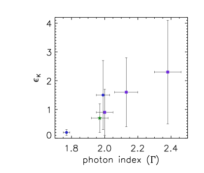
Figure 9.— Outflow efficiency ($\epsilon_{K}$) of the outflow versus photon index ($\Gamma$) for our eight observations of APM 08279+5255. $\epsilon_{K}$ and $\Gamma$ were derived from fits to the spectra of APM 08279+5255 with a model that included an absorbed power-law and two component outflow (MODEL2 of Tables 3 and 4) for the Suzaku and Chandra observations and a single component outflow for the XMM-Newton observations (MODEL1 of Table 4). Errors shown are at the 68% confidence level. The Suzaku data points are displayed as a single point that represents the weighted (by total counts) mean of the three Suzaku observations. Data shown with circles, a star, and squares are obtained from Chandra, Suzaku and XMM-Newton observations respectively.

In Table 6 we show the mass outflow rate ($\dot{M}$) and the efficiency ($\epsilon_{K}$) of the wind in each observation. The parameters used in equations (4) and (5) to derive $\dot{M}$ and $\epsilon_{K}$ were obtained from spectral fits of MODEL2 to the Suzaku and Chandra observations, and through the use of MODEL1 for the XMM-Newton observations (see Tables 3 and 4). For the Suzaku and Chandra observations we estimate $\dot{M}$ and $\epsilon_{K}$ for the slow and fast component of the outflow. The total mass outflow rate and efficiency is obtained by summing the contributions of the slow and fast outflow component (MODEL2, § 3.3.2) when multiple components are required to fit the data. In the case of the XMM-Newton observations no summing is required since a one component wind model (MODEL1, § 3.3.2) provides better fits (in a statistical sense) to the spectra of APM 08279+5255 (see § 3.3.2). In Table 6, assuming that the outflow is viewed along our line of sight, we show that during the observations of APM 08279+5255 the total mass outflow rate varied between $21^{+19}_{-13}-65^{+58}_{-41}$ $M_{\odot}{\rm yr}^{-1}$ ($\mu_{L}=100$) and the total efficiency varied between $0.2^{+0.2}_{-0.1}-2.3^{+2.1}_{-1.5}$. However, the total values of $\dot{M}$ and $\epsilon_{K}$ are $\sim 10\%$ and $\sim 50\%$ higher respectively if we assume an outflow forming an angle of $10^{\circ}$ with our line of sight (see Table 6). In Table 6 we also show that an important fraction ($>10\%$) of the bolometric energy of APM 08279+5255 is injected into the surrounding galaxy through quasar winds.

As Figure 8 shows the softer spectra probably result in a faster and more massive (higher total column density) wind. This tendency can be seen more clearly in Figure 9 where we have plotted the total efficiency ($\epsilon_{K}$) as a function of the photon index ($\Gamma$). We note that a small contribution to the error bars ($\lesssim 20\%$) of $\epsilon_{K}$ arises from errors in the fitted parameters (i.e., $v_{\rm min}$, $v_{\rm max}$ and log $N_{\rm H}$) while most of the error in $\epsilon_{K}$ is due to the uncertainty of $R$, $f_{c}$, $R/\Delta R$.

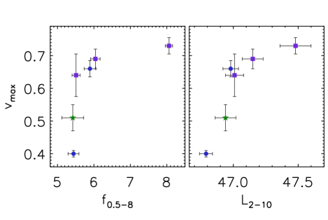
Figure 10.— Maximum velocity ($v_{\rm max}$; upper panel) versus absorbed flux in the 0.5$-$8 keV band ($f_{0.5-8}$; left panel) and intrinsic luminosity in the 2$-$10 keV rest-frame  band ($L_{2-10}$; right panel) for our eight deep observations. $v_{\rm max}$ and $L_{2-10}$ were derived from fits to the spectra of APM 08279+5255 with a model that included an absorbed power-law and two component outflow (MODEL2 of Tables 3 and 4) for the Suzaku and Chandra observations and a single component outflow for the XMM-Newton observations (MODEL1 of Table 4). The absorbed fluxes in the 0.5$-$8 keV band are from Table 1. Errors shown are at the 68% confidence level. In each panel the Suzaku data points are displayed as a single point that represents the weighted (by total counts) mean of the three Suzaku observations. Data shown with circles, a star, and squares are obtained from Chandra, Suzaku and XMM-Newton observations respectively.

The 0.5$-$8 keV flux of APM 08279+5255  varies by up to 50% in the observations of our study (see Table 1). These flux changes appear to be correlated to changes of the maximum outflow velocity (see Figure 10; left panel). The observed changes in flux may be caused by changes in the luminosity of the ionizing source. By fitting our outflow model to the X-ray spectra of APM 08279+5255 we obtain the intrinsic (unabsorbed) 2$-$10 keV rest-frame X-ray luminosity of the ionization source ($L_{2-10}$) (see Tables 3 and 4). We find that the maximum velocity of the outflow is possibly correlated to the intrinsic luminosity of the ionizing source (see Figure 10; right panel). From the radiative outflow wind equation we obtain that the terminal velocity of the wind is $v_{\infty}\propto\sqrt{\Gamma_{f}L}$, where $L$ is the luminosity producing the radiative driving and $\Gamma_{f}$ is the force multiplier (see §4 for an analysis describing the dependence of $\Gamma_{f}$ with the photon index). This equation predicts that an increase in the luminosity of the ionizing source should result in an increase of the terminal velocity of the outflow as observed. The Suzaku observations of APM 08279+5255 do not show any significant changes of $\Gamma$, $v_{\rm max}$, the total column density, and $L_{2-10}$ (see Table 3). In Figures 8, 9 and 10 we therefore chose to represent the Suzaku observations with one data point. The Suzaku data point in each figure is the weighted mean of the three Suzaku observations.

As a final comment, the ionization parameter obtained from the spectral fits is based on the assumption that the incident spectrum is a pure power-law with a fixed slope ($\alpha=-1$). In reality the spectra are likely more complex and variable than assumed in our model. Our simple approach provides reliable constrains on the column density and velocity of the outflow. However, since the ionization parameter depends on the SED from 1$-$1000 Ry (see Appendix A) we do not expect that fits of our quasar outflow model to the spectra of APM 08279 +5255 to constrain the ionization parameter since our model assumes a fixed SED. What our model does constrain is the temperature of the absorber which is a reliable indicator of the degree of ionization of the outflowing gas.

4. Influence of the SED on the dynamics of the outflow

In section 3 we presented a quasar outflow model that was fit to X-ray observations of APM 08279+5255 in order to constrain the column densities of the absorbers, their ionization state and their outflow velocities. The outflow models used to fit these X-ray data assumed that the incident SED is a power law with a spectral index of $\alpha=-1$. In this section we attempt to understand the influence of the incident SED on the dynamics of the outflow. We vary the SED to obtain insight into the dependence of the force multiplier on the incident SED, however, we do not fit any data with variable SEDs. This section extends the analysis presented in §3.3 from Chartas et al. (2009a) by providing an analysis of force multipliers as a function of the spectral changes of a Mathews-Ferland SED, while, in the Chartas et al. (2009a) paper we performed the same analysis but using a pure power-law SED. Here we focus on the new results that are based on more realistic SEDs.

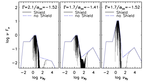
Figure 11.— Modified Mathews-Ferland SEDs used to calculate force-multipliers in §4.1. The x-axis is the logarithm of frequency (in Ry units) and the y-axis is in units of the logarithm of the flux times the frequency (arbitrary units). The left and right panels correspond to two modified versions of the Mathews-Ferland SED. In the left and right panels $\Gamma=2.1$ and $\Gamma=1.7$ with $\hbox{$\alpha_{\rm ox}$}=-1.52$. The middle panel corresponds to the standard Mathews-Ferland SED, i.e. $\Gamma=1.7$ with $\hbox{$\alpha_{\rm ox}$}=-1.41$. In each panel the dotted line is the unabsorbed SED and the solid line is the shielded SED (with $\hbox{log~{}$\xi$}_{\rm sh}\sim 2.9$).

4.1. The dependence of the force multiplier on the photon index and $\alpha_{\rm ox}$  for a Mathews-Ferland SED.

As suggested in Chartas et al. 2002, 2009a and Saez et al. 2009 it is plausible that the driving force on the high-energy absorbers is produced initially by X-rays. The short term variability time-scale of the X-ray BALs of APM 08279+5255 suggests a launching radius of $\lesssim$ $10R_{\rm S}$ and recent studies of AGN employing the microlensing technique indicate that the X-ray emission region of the hot corona in AGNs is compact with a half-light radius of a few $R_{\rm S}$ and their UV regions are roughly a factor of ten larger (e.g., Morgan et al., 2008; Chartas, 2009b). Therefore UV radiation is not expected to contribute initially at small radii to driving the X-ray absorbing outflow. However, as the outflowing absorber gets further away from the source the contribution of the UV photons to the driving force will increase relative to that of the X-ray photons. To investigate the driving mechanism of the wind we calculated the force multipliers for SEDs that extend to radio wavelengths and estimated the effect of changes in $\Gamma$. In Chartas et al. (2009a) we described the dependence of the force multiplier on the photon index assuming the SED is a power-law extending from the UV (or 1 Ryd $\sim$13.6 eV) to hard X-rays (or $10^{4}$ Ryd $\sim$100 keV). In those calculations we assume SEDs with two different values of the power-law photon index. A “soft” ($\Gamma=2.1$) and a “hard” ($\Gamma=1.7$) SED. In this work we extend our simulations to include a standard and a slightly modified version of the Mathews-Ferland SED (Mathews & Ferland, 1987). For each SED we calculated the continuum ($M_{\rm C}$) and the line ($M_{\rm L}$) components of the force multiplier. $M_{L}$ depends on an additional parameter, $t$, which is commonly referred to as the “effective electron optical depth” and encodes the dynamical information of the wind in the radiative acceleration calculation (see Appendix E). For our calculations we have assumed ${\rm log}~{}t=-7$.

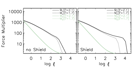
Figure 12.— The bound-free, $M_{\rm C}$, and bound-bound, $M_{\rm L}$, components of the force multiplier are shown as a function of the ionization parameter. Force multipliers are calculated for Mathews-Ferland SEDs with photon indices of $\Gamma$ = 2.1 (solid lines) and $\Gamma$ = 1.7 (dotted lines). In the left panel we have assumed no absorbing shield, whereas, in the right panel the soft and hard SEDs have been attenuated by a warm-absorber shield with $\hbox{log~{}($N_{\rm H}/{\rm cm}^{-2})$}=23$ and $\hbox{log~{}$\xi$}_{\rm sh}=2.9$ on its illuminated face. The SEDs used are described by the middle and right panels of Figure 11.

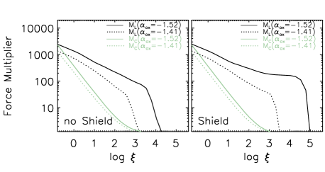
Figure 13.— The bound-free, $M_{\rm C}$, and bound-bound, $M_{\rm L}$, components of the force multiplier are shown as a function of the ionization parameter. Force multipliers are calculated for a Mathews-Ferland SED with $\hbox{$\alpha_{\rm ox}$}=-1.52$ (solid lines) and $\hbox{$\alpha_{\rm ox}$}=-1.41$ (dotted lines); in both SEDs $\Gamma=1.7$. In the left panel we have assumed no absorbing shield, whereas, in the right panel the soft and hard SEDs have been attenuated by a warm-absorber shield with $\hbox{log~{}($N_{\rm H}/{\rm cm}^{-2})$}=23$ and $\hbox{log~{}$\xi$}_{\rm sh}=2.9$ on its illuminated face. The SEDs used are described by the middle and left panel of Figure 11.

The standard Mathews-Ferland SED is characterized by $\hbox{$\alpha_{\rm ox}$}=-1.41$ and by a power-law spectral index of $\alpha_{X}=-0.7$ ($\Gamma=1.7$) which extends from 27 Ry ($\sim$0.36 keV) to 7.4$\times 10^{3}$ Ry ($\sim$100 keV). The modified Mathews-Ferland SED is similar to the standard one but with $\alpha_{X}=-1.1$ and $\hbox{$\alpha_{\rm ox}$}=-1.52$ (see Figure 11 to see the different SEDs used). In the left panel of Figure 12 we show that for low ionization parameters ($\hbox{log~{}$\xi$}\lesssim 2$) the UV dominates the driving of the wind, therefore in this regime there is no major change in the force multipliers when we compare the soft and hard Mathews-Ferland SEDs. However at $\hbox{log~{}$\xi$}\gtrsim 2$, the line force multipliers for the soft Mathews-Ferland SED case are larger than those for the hard SED case. This effect is produced because in the case of a Mathews-Ferland SED with a soft X-ray spectrum ($\Gamma=2.1$) the outflowing gas does not become very ionized at high levels of the ionization parameter compared to the case of a Mathews-Ferland SED with a hard X-ray spectrum ($\Gamma=1.7$). We conclude that an ionizing source that is relatively soft in the X-ray band will result in a force multiplier that remains relatively large even at ionization levels of the outflowing absorber of $\hbox{log~{}$\xi$}\gtrsim 3$. This prediction is consistent with the observed correlation of maximum outflow velocity with the X-ray photon index. We modified the SEDs by including a warm-absorber shield with $\hbox{log~{}($N_{\rm H}/{\rm cm}^{-2})$}=23$ and $\hbox{log~{}$\xi$}_{\rm sh}=3.1$ (Figure 12 right panel; see also Figure 11 to see the shielded SED). The motivation of the inclusion of this absorbing shield is based on the fact that both observations and theoretical models of radiatively driven winds suggest its existence (e.g., Murray et al., 1995; Proga et al., 2004). We note that the observed absorption at rest-frame energies $\lesssim 2$ keV appears to be produced by gas of low ionization parameter and could therefore be associated with this proposed shield. The main effect of including a shield is a larger increase of the line force multipliers for the soft SED case ($\Gamma=2.1$) compared to the increase produced by the hard SED case ($\Gamma=1.7$) for $\hbox{log~{}$\xi$}\gtrsim 2$. We also find that by including a shield we obtain significant line force multipliers at ionization levels that are larger than the ones possible with no shield present. This effect is especially important in the soft SED case.

In the process of changing the X-ray photon index from the default value of $\Gamma=1.7$ (hard-spectrum) to $\Gamma=2.1$ (soft spectrum) in the Mathews-Ferland SED, we also changed $\alpha_{\rm ox}$ from $-1.41$ to $-1.52$. To test the sensitivity of the force multiplier to changes of the $\alpha_{\rm ox}$ of the SED, we estimated the force multiplier for the case where $\alpha_{\rm ox}$ changed while the X-ray spectral slope remained constant. In order to produce this effect we increased the blue bump of the Mathews-Ferland SED by changing the default value of $\alpha_{\rm ox}$ from $-1.41$ to $-1.52$ (to see the SEDs used see Figure 11). As shown in the left panel of Figure 13 the force multiplier is more sensitive to $\alpha_{\rm ox}$ than $\Gamma$. This difference in sensitivity is associated with the fact that the UV covers the range where most of the absorption lines lie. We also modified the SEDs by including an absorbing shield with $\hbox{log~{}($N_{\rm H}/{\rm cm}^{-2})$}=23$ and $\hbox{log~{}$\xi$}_{\rm sh}=3.1$ (see Figure 11). In the right panel of Figure 13 we show that the effect of adding this warm-absorber shield is an increase of the force multiplier for soft SEDs even at high ionization levels.

We note that we used a moderate amount of shielding for the estimates shown in the left panels of Figures 12 and 13. The combination of moderate attenuation and high force multipliers in this type of shield is expected to produce high velocity outflows (Chelouche & Netzer, 2003). If we use an absorbing shield with a relatively low ionization level we find that the large absorption from the shield will attenuate a large fraction of the UV and X-ray photons, and therefore prevent the outflow from reaching high terminal velocities.

In general, the presence of an absorbing shield will increase the differences between the line force multipliers for the soft and hard SED cases. These differences will be important for shields with ionization parameters in the range of $1.0\lesssim\hbox{log~{}$\xi$}_{\rm sh}\lesssim 1.8$ for the power-law SED case and will be important for shields with ionization parameters in the range of $1.2\lesssim\hbox{log~{}$\xi$}_{\rm sh}\lesssim 3.1$ for the Mathews-Ferland SED case (see Appendix F). For values of the ionization parameter of the shield over these boundaries, the shield will be transparent to incident radiation and the force multipliers will be similar to ones with no shield present (left panels of Figures 12 and 13). For values of $\hbox{log~{}$\xi$}_{\rm sh}\lesssim 1.0$ the large absorption produced by the shield will result in a weak outflow (see, Chelouche & Netzer, 2003).

If the $\Gamma-v_{\rm max}$ trend is confirmed with additional observations we plan to produce a more sophisticated model that will include more realistic kinematic, ionization and absorption properties of the outflow. If the $\Gamma-v_{\rm max}$ relation is real we would also like to know if the changes in $\Gamma$ are accompanied by changes of $\alpha_{ox}$. Studies of correlations between outflow properties and the SED of the ionizing source will provide crucial information regarding the driving mechanism of the outflow. Simultaneous multiwavelength observations of sources such as APM 08279+5255 that show fast outflows will therefore be essential for the study of quasar outflows. We note that for the SEDs analyzed in this section the contribution to the force multiplier from highly ionized iron lines such as Fe xxv  K$\alpha$ ($1s^{2}-1s2p$; 6.70 keV) and/or Fe xxvi  ($1s-2p$; 6.97 keV) is relatively small. However, we observe significant blueshifts of the X-ray BALs of APM 08279+5255 indicating highly ionized material moving at near-relativistic velocities. One possible interpretation is that we are observing absorption from outflowing highly ionized material that was accelerated at a previous time when it was at a lower ionization level. We note that a better understanding of quasar outflows will have to await for the development of more sophisticated numerical codes that combine MHD simulations of the outflowing material and the photoionization properties of the wind. Such an analysis is beyond the scope of this paper.

5. Conclusions

We have re-analyzed 8 long exposure X-ray observations of APM 08279+5255 (2 Chandra, 3 XMM-Newton, and 3 Suzaku) using a new quasar-outflow model. This model is based on cloudy simulations of a near-relativistic quasar outflow that were used to generate xspec table models.

The main conclusions from this re-analysis are: 1) In each observation we have found X-ray BALs that have been detected at a high level of significance. Specifically, we find strong and broad absorption at rest-frame energies of $1-4$ keV (low-energy) and $7-18$ keV (high-energy). 2) We confirm that the medium producing the low-energy absorption is a nearly neutral absorber with a column density of $\hbox{log~{}($N_{\rm H}/{\rm cm}^{-2})$}\sim 23$. The medium producing the high-energy absorption appears to be outflowing from the central source at relativistic velocities (between $0-0.7c$) and with a range of ionization parameters ($3\lesssim\hbox{log~{}$\xi$}\lesssim 4$). The maximum detected projected outflow velocity of $\sim 0.7c$ constrains the angle between our line of sight and the wind direction to be $\lesssim 22^{\circ}$. The short time-scale variability ($\lesssim$ week in the rest-frame) of the high-energy absorption implies that X-ray absorbers are launched from distances of $\sim 10R_{S}$ from the central source (where $R_{S}$ is the Schwarzschild radius). 3) We also confirm trends between the maximum projected outflow velocity ($v_{\rm max}$) with the photon index ($\Gamma$) and the intrinsic (unabsorbed) X-ray luminosity at the 2$-$10 rest-frame band; i.e. softer and more luminous X-ray spectra generate larger outflow terminal velocities. We also find that the total column density (${N}_{\rm H}$) of the outflow increases with $\Gamma$. The trends found suggest that the wind becomes more powerful as the incident spectrum becomes softer. This tendency is confirmed through estimates of the efficiency of the wind. Additionally, we estimate that a significant fraction ($>$10%) of the total bolometric energy over the quasar’s lifetime is injected into the intergalactic medium of APM 08279+5255 in the form of kinetic energy.

In this work we modeled the spectrum of the central ionizing source with a power-law SED and with Mathews-Ferland SEDs and found that variations of the X-ray and UV parts of the SEDs will produce important changes in the strength of the radiative driving force. These results support the observed trend found between the outflow velocity and X-ray photon index in APM 08279+5255. In general we find as expected that the presence of a moderate absorbing shield results in more powerful outflows (Chelouche & Netzer, 2003). Specifically, we find that shields with column densities of $\hbox{log~{}($N_{\rm H}/{\rm cm}^{-2})$}\sim 23$, covering an optically thin outflow, provide a significant increase in the driving force when their ionization parameters are in the range of $1.0\lesssim\hbox{log~{}$\xi$}_{\rm sh}\lesssim 1.8$ for the case of a power-law SED and in the range of $1.2\lesssim\hbox{log~{}$\xi$}_{\rm sh}\lesssim 3.1$ for the case of a Mathews-Ferland SED. Therefore the strength of the radiative driving force depends critically on both the column density of the shield and its ionization level. A confirmation of the results found in our simulations of quasar outflow will require new deeper X-ray  multi-wavelegth observations of quasars that contain clear signs of fast outflow. Such observations will allow us to correlate the properties of the outflow with properties of the SED and thus test our predictions.

Appendix A Ionization parameter.

There are two definitions of the ionization parameter that are broadly used in the scientific literature. The first definition, which will be mostly adopted in this work, is the ionization parameter of Tarter, Tucker & Salpeter (1969) given by

$$\xi=\frac{L_{\rm I}}{n_{H}r^{2}}=\frac{4\pi}{n_{H}}\int_{1\rm Ry}^{1000\rm Ry}F_{\nu}d\nu=\frac{4\pi F_{I}}{n_{H}},$$ (A1)

where $L_{I}$ is the ionizing luminosity, $F_{I}$ is the ionizing flux, $F_{\nu}$ is the incident flux, $n_{H}$ is the hydrogen density, and $r$ is the source-cloud separation. A second definition of the ionization (Davidson, 1977) parameter is given by the ratio of photons that can ionize hydrogen to the number of hydrogen atoms in a spherical layer at a distance $r$ from an illuminating point source, i.e.,

$$U=\frac{Q}{4\pi r^{2}cn_{H}}\hskip 10.0pt,{\rm where}\hskip 10.0ptQ=\int_{1\rm Ry}^{\infty}\frac{L_{\nu}}{h\nu}d\nu.$$ (A2)

We note that for a pure power law (i.e., $F_{\nu}\propto\nu^{\alpha}$), the analytic expressions to convert between $\xi$ and $U$ (valid for $\alpha<0$) are,

$$\hbox{log~{}$\xi$}=\left\{\begin{array}[]{ll}\hbox{log~{}$U$}+1.754&\alpha=-1\\ \hbox{log~{}$U$}+0.914+{\rm log}\left(-(1000^{\alpha+1}-1)\frac{\alpha}{\alpha+1}\right)&\alpha\neq-1\end{array}\right.$$ (A3)

Appendix B When can an absorption slab be considered thin?

The fraction of flux absorbed in the rest-frame of a layer of gas depends on the ionization state of the absorber, its column density, and the SED of the illuminating source. Our quasar outflow code calculates the absorption profiles resulting from absorption of the central source spectrum by ionized gas in an accelerated outflow. One of the assumptions of our quasar outflow model is that the absorption layer producing the observed X-ray BALs has a plane-parallel geometry with a thickness that is much smaller than the distance from the central source. We therefore expect any decrease in the ionization parameter across an absorbing layer to be predominantly due to the absorption of the flux in the layer rather than to the 1/R² decrease of the ionization parameter.

We will refer to a layer as optically thin if the change between the ionization parameter on the illuminated side and the dark side of the layer is less than 0.05 dex.

Figure A.1.— Limiting column density at which a layer will be considered thin. In this case we arbitrarily define a layer as thin when the ionization parameter decreases after crossing the layer less than 0.05 dex due to absorption. The solid and dotted lines represent a soft spectrum power-law ($\Gamma=2.2$) and hard power-law spectrum ($\Gamma=1.5$), respectively. Both spectra are defined between 1 Ry and $10^{4}$ Ry

In Figure A.1 we show the column density of a thin layer that will produce a decrease of 0.05 dex of the ionization parameter across this layer as a function of the ionization parameter at the front surface of the layer. We plot this relation for power-law SEDs with a photon index of $\Gamma=1.5$ (dotted line) and with $\Gamma=2.2$ (solid line). The results show that the upper limit of the column density of an absorbing layer required for this layer to be considered thin, increases with ionization parameter. Soft spectra have lower thresholds than hard spectra, especially for low values of the ionization parameter ($\hbox{log~{}$\xi$}\lesssim 2$). However, for highly ionized media the threshold of the soft and hard spectra are similar, in particular for ($\hbox{log~{}$\xi$}\gtrsim 3$) the limiting column density is $\hbox{log~{}($N_{\rm H}/{\rm cm}^{-2})$}\sim 23$.

Appendix C Near-relativistic quasar outflow code: assuming an outflow with a constant $\Delta v^{\prime}$ between layers

Since our library of cloudy simulations was generated for a specific turbulent velocity we adjusted the relative speed between layers $i$ and $i+1$ to be constant (i.e. $\Delta v_{i}^{\prime}=(v_{i+1}-v_{i})/(1-v_{i}v_{i+1}/c^{2})$ constant). Assuming $N_{l}$ layers, we initialize the parameters defining our profile by: 1) Deriving the velocity profile, which satisfies $v_{0}=v_{\rm min}$; $v_{N_{l}}=v_{\rm max}$ ($\Delta v_{i}^{\prime}=\Delta v^{\prime}$). 2)Deriving $\hbox{${N}_{\rm H}$}_{i}$ (i=0,..,$N_{l}$) through the use of $\hbox{${N}_{\rm H}$}_{i+1}^{p}-\hbox{${N}_{\rm H}$}_{i}^{p}=\Delta v_{i}/k$; this result comes from $v(\hbox{${N}_{\rm H}$})=v_{\rm min}+k\hbox{${N}_{\rm H}$}^{p}$ ($k=(v_{\rm max}-v_{\rm min})/\hbox{${N}_{\rm H}$}_{T}^{p}$ and $\hbox{${N}_{\rm H}$}_{T}$ is the total column density of the outflow). Using the last expression we calculate $\hbox{${N}_{\rm H}$}_{i}$ from $\hbox{${N}_{\rm H}$}_{i-1}$ starting from $\hbox{${N}_{\rm H}$}_{0}=0$. 3) Calculating the average velocity $v_{mi}=(v(r_{i+1})+v(r_{i}))/2$, the column density $\Delta\hbox{${N}_{\rm H}$}_{i}=\hbox{${N}_{\rm H}$}_{i+1}-\hbox{${N}_{\rm H}$}_{i}$, the density $n_{i}=n(v_{mi})$, (i=0,..,$N_{l-1}$) and the radial steps $\Delta r_{i}=\Delta\hbox{${N}_{\rm H}$}/n_{i}$ of each layer.

We note that our assumptions are valid as long as $\Delta v<v_{\rm turb}\sqrt{12}$ (see §3.2.3). In our simulations we chose $\Delta v_{i}\sim v_{\rm turb}$ and $v_{\rm turb}=1500~{}\hbox{km~{}s${}^{-1}$}\sim 0.005c$ . In the case of $v_{\rm min}=0.1c$ and $v_{\rm max}=0.7c$ we would have $N_{l}\sim 100$ layers.

Appendix D Near-relativistic quasar outflow code: comparison with Schurch & Done (2007)

In this appendix we compare our quasar outflow code to a similar code presented in Schurch & Done (2007). The goal is to estimate the level of agreement between two independent quasar outflow codes and at the same time evaluate the limitations of each approach. We first generated absorption profiles for a linearly accelerated outflow ($p=1$) with $v_{\rm min}=0$, $v_{\rm max}=0.3c$, $\hbox{${N}_{\rm H}$}=3\times 10^{23}$ cm^-2, $n_{0}=10^{12}$ cm^-3, and values of $\hbox{log~{}$\xi$}=$ 2.75, 3, 3.25, 3.5, 3.75 and 4. In order to make a fair comparison with the results of Schurch & Done (2007) we ran a large number of simulations using the photoionization code xstar and assumed a power-law model with $\alpha=-1.4$.

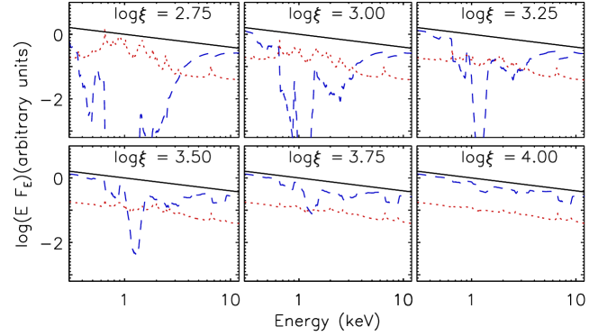
Figure A.2.— 0.3-13 keV spectra of the incident (full-line), transmitted (dashed-line) and emitted (dotted-line) continua for different ionization levels of the outflowing material simulated with our quasar outflow code. In Panels 1-3 (Top, left to right) the ionization levels of the outflowing material are log $\xi$= 2.75, 3.0 & 3.25, respectively. In Panels 4-6 (Bottom, left to right) the ionization levels of the outflowing material are log $\xi$= 2.75, 3.0 & 3.25, respectively. For all these simulations the total number of layers is $N_{l}=100$, the total column density of the outflowing material is $N_{\rm H}=3\times 10^{23}$ cm^-2, the initial gas density is 10¹² cm^-3 and the velocity of the outflow is assumed to vary linearly between 0 and 0.3 $c$. These results are in good agreement with those of Schurch & Done (2007) as evident from a comparison between this figure and their Figure 7.

In each layer we subtract the absorption an add the emission. Since xstar does not include a “Compton scattered” component for the emission, we add this component in a similar way as the one described in Schurch & Done 2007. The Compton scattered emission component is obtained by calculating the Thomson scattered flux of each layer, where the incident spectrum is the output from the previous layer. Since in the case of Schurch & Done (2007) the calculations were made assuming spherical symmetry of the multilayer absorber, with global covering factors equal to one, we use similar assumptions to obtain the emission of each layer. We calculated the emission from a spherical shell by adding the spectral contribution from each solid angle of the layer. The emission from each solid angle of the shell is corrected for Doppler beaming of material outflowing at a projected velocity with respect to a fixed line of sight.

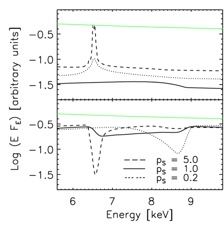
Figure A.3.— Emitted (upper panel) and absorbed (lower panel) spectra in the energy range where we detect iron absorption ($\sim$7–9 keV) for three different values of the exponent of the $p$-type velocity profile, (see equation 3, §3) of $p$ = 5.0, 1.0 and 0.2. For these comparison tests we set $v_{\rm min}=0$, $v_{\rm max}=0.3c$, $\hbox{${N}_{\rm H}$}=3\times 10^{23}$ cm^-2, $n_{0}=10^{12}$ cm^-3, and $\hbox{log~{}$\xi$}=3$. We find agreement between our code and that of Schurch & Done 2007 as shown in the comparison between the absorption and emission profiles presented in Figure A.3 and Figure 4 of Schurch & Done (2007).

The spectra of the incident, absorbed and emitted continua for each of the initial values of the ionization parameters used in these calculations of absorption line profiles are presented in the six panels of Figure A.2. We find a remarkable similarity of Figure A.2 with Figure 7 of Schurch & Done 2007. The small differences found in our results when compared to those of Schurch & Done (2007) are mainly associated with differences in the details of the calculations. Specifically, Schurch & Done 2007 pass the output flux from one layer to the other internally, while in our approach we perform separate photoionization runs from one layer to the next. Possibly an important factor that contributes to the discrepancies between the two codes is that in our calculations we approximate the incident flux on each layer as being the unabsorbed source SED. On the other hand, Schurch & Done (2007) use the absorbed SED to perform the photoionization calculations in each layer. We expect our approximation of using the unabsorbed source SED as incident on all layers to break down at low ionization levels where absorption through a layer may significantly change the SED. This explains why our results begin to noticeably differ from those of Schurch & Done (2007) at $\hbox{log~{}$\xi$}\lesssim 3$.

In Figure A.3 we plot the absorbed and emitted spectra in the energy range where we detect iron absorption ($\sim$7–9 keV) for three different values of the exponent of the $p$-type velocity profile, (see equation 3, §3) of $p$ = 5.0, 1.0 and 0.2. For these comparison tests we set $v_{\rm min}=0$, $v_{\rm max}=0.3c$, $\hbox{${N}_{\rm H}$}=3\times 10^{23}$ cm^-2, $n_{0}=10^{12}$ cm^-3, and $\hbox{log~{}$\xi$}=3$. We find agreement between our code and that of Schurch & Done 2007 as shown in the comparison between the absorption and emission profiles presented in Figure A.3 and Figure 4 of Schurch & Done (2007). Our emission spectra for the case of a velocity profile with an exponent of $p=5$ differs from those derived by Schurch & Done 2007 (see Figure 4 of Schurch & Done (2007)) mainly because in their simulations the turbulent velocity is set to be variable in order to model fine structures in the spectra. In our simulations we fix the turbulent velocity in the outflow, and therefore we are not able to reproduce fine details ($\lesssim 1500$ km s^-1) in the spectra. This is not a significant problem since we are mainly interested in simulating the broad absorption lines detected in the X-ray spectra of BAL quasars.

We conclude that our quasar outflow code provides results that are very similar to those found in the independent code of Schurch & Done 2007 as long as the SED does not change significantly across the multilayer. For our study we have mostly selected quasar outflows of highly ionized material (i.e., log $\xi$ $\gtrsim 3.0$ ) and therefore expect the SED of the central source not to be significantly attenuated across the outflowing multilayer. As a final remark, we note that in our quasar outflow code the photoionization calculations at each layer use a library of preexisting runs that can be performed either with cloudy  xstar or any other photoionization code. This presents an advantage over the quasar outflow code xscort in the sense that we can compare photoionization calculations performed with different photoionization codes which might incorporate slightly different atomic physics. Additionally, the major advantage of using our outflow code over xscort, is a significant shortening in the computing time required for the simulation of an absorption profile.

Appendix E Force multiplier calculations

In this appendix we derive a formula for the force multiplier and compare our expression to ones reported in earlier studies (see e.g., Arav et al., 1994; Mihalas & Mihalas, 1984).

E.0.1 Force multiplier calculation

For a medium that absorbs radiation, the force per unit volume on the medium is

$$f_{v}=\frac{1}{c}\int\alpha_{\nu}F_{\nu}d\nu,$$ (E1)

where $\alpha_{\nu}$(cm^-1) is the absorption coefficient and $F_{\nu}$ is the incident flux on the medium. Assuming that the flux originates from a point source with luminosity $L_{\nu}$ at $r=0$ the acceleration is given by

$$\frac{dv(r)}{dt}=\frac{1}{4\pi r^{2}\rho(r)c}\int\alpha_{\nu}L_{\nu}e^{-\tau_{\nu}}d\nu.$$ (E2)

The factor $e^{-\tau_{\nu}}$ corresponds to the attenuation factor at radius r, ($\tau_{\nu}(r)=\int_{0}^{r}\alpha_{\nu}(r^{\prime})dr^{\prime}$). Assuming that the central source has a mass of $M_{s}$ the force equation can be re-written as:

$$\frac{dv(r)}{dt}=\frac{n_{e}(r)\sigma_{\rm T}L_{\rm bol}}{4\pi r^{2}\rho(r)c}M(r)-\frac{GM_{s}}{r^{2}}\hskip 10.0pt{\rm with}\hskip 10.0ptM(r)=\frac{\int_{0}^{\infty}\alpha_{\nu}(r)L_{\nu}e^{-\tau_{\nu}(r)}d\nu}{n_{e}(r)\sigma_{T}L_{\rm bol}},$$ (E3)

where $L_{\rm bol}$ is the bolometric luminosity, $\sigma_{T}$ is the Thomson cross section and $M(r)$ is the force multiplier. $M(r)$ can be interpreted as the ratio of energy absorbed by the medium to the energy absorbed by the electrons.

As a simple example we assume that the medium is a spherical shell with inner and outer radii of $R$ and $R+\Delta R$, respectively. For this case $\left<M(r)\right>=\int M(r)dr/\Delta R$; and therefore, the wind equation (E3) is approximated as

$$\frac{dv(r)}{dt}=\frac{\sigma_{\rm T}L_{\rm bol}}{1.2m_{\rm p}4\pi r^{2}c}\left<M(r)\right>-\frac{GM_{s}}{r^{2}}$$ (E4)

In this last stage we have assumed a high ionization state for the gas at solar metallicities and therefore $\rho_{r}/n_{e}(r)\sim 1.2m_{\rm p}$, where $m_{\rm p}$ is the mass of the proton. Assuming that $v(R_{\rm min})=0$ the solution of equation (E4) is

$$v(r)=\sqrt{2GM_{s}\left(\frac{L_{\rm bol}}{1.2L_{\rm Edd}}\left<M\right>-1\right)\left(\frac{1}{r_{\rm min}}-\frac{1}{r}\right)}$$ (E5)

where $L_{\rm Edd}$ is the Eddington Luminosity (i.e. $L_{\rm Edd}=\frac{4\pi cG\mu m_{p}M_{s}}{\sigma_{T}}$).

To calculate the force multiplier of a line we start from equation (E3). Let’s assume that the absorption line has a constant opacity, frequency $\nu_{l}$ and a width $\Delta\nu_{\rm th}=\nu_{l}v_{\rm th}/c$ (where $v_{\rm th}$ is the thermal speed of the absorbing atoms). The characteristic distances of radiative interactions are of the order of $l\sim v_{\rm th}/(\nabla v)$. Hence for radially streaming radiation in an expanding medium the optical thickness is,

$$\tau_{l}=\alpha_{l}v_{\rm th}/(dv/dr)$$ (E6)

where $\alpha_{l}$ is the absorption coefficient of the line. We define $\eta_{l}=\frac{\alpha_{l}}{n_{e}\sigma_{T}}$ and introduce an equivalent electron optical depth scale

$$t=\tau_{l}/\eta_{l}=n_{e}\sigma_{T}v_{\rm th}/(dv/dr).$$ (E7)

Therefore the mean force multiplier is $\left<M(r)\right>=\int M(r)dr/l$, i.e.,

$$\left<M(r)\right>=\frac{\int_{r}^{r+l}M(r)dr}{l}=\frac{L_{\nu_{l}}\Delta\nu_{th}(1-e^{-\tau_{l}})}{n_{e}\sigma_{T}l~{}L_{\rm bol}}.$$ (E8)

Summing up over all absorption lines we obtain

$$M(t)=\frac{1}{L_{\rm bol}}\sum_{l}\frac{L_{\nu_{l}}\Delta\nu_{th,l}(1-e^{-\eta_{l}t})}{t}\approx\frac{1}{L_{\rm bol}}\sum_{l}L_{\nu_{l}}\Delta\nu_{th,l}~{}{\rm min}\left(\eta_{l},\frac{1}{t}\right).$$ (E9)

To obtain $\alpha_{l}$ we use equation 1.78 from Rybicki & Lightman (1985) i.e.,

$$\alpha_{l}=\frac{h\nu_{l}}{4\pi}n_{l}B_{lu}\left(1-\frac{g_{l}n_{u}}{g_{u}n_{l}}\right)\phi(\nu).$$ (E10)

Assuming that the absorption line has a square-topped profile of width $\Delta\nu_{\rm th,l}$, $\phi=\frac{1}{\Delta v_{\rm th,l}}$, and using $B_{lu}=\frac{4\pi^{2}e^{2}}{h\nu_{l}mc}f_{l}$, where $f_{l}$ is the oscillator strength we obtain

$$\alpha_{l}=\frac{\pi e^{2}}{m_{e}c}g_{l}f_{l}\frac{(n_{l}/g_{l}-n_{u}/g_{u})}{\Delta\nu_{th,l}}.$$ (E11)

Inserting equation E11 into E9 we reproduce the result of Arav et al. (1994), i.e.,

$$M(t)=\frac{1}{L_{\rm bol}}\sum_{l}L_{\nu_{l}}\Delta\nu_{th,l}\frac{1-e^{-\eta_{l}t}}{t}\hskip 20.0pt{\rm with}\hskip 20.0pt\eta_{l}=\frac{\pi e^{2}}{m_{e}c}gf_{l}\frac{(n_{l}/g_{l}-n_{u}/g_{u})}{n_{e}\sigma_{T}\Delta\nu_{th,l}}.$$ (E12)

E.1. Comparison with other results.

The force multiplier mainly depends on the SED of the source, the composition of the gas, and its ionization parameter. In general a soft spectrum irradiating a gas that is nearly neutral (i.e. low ionization parameter) will strongly accelerate the gas and the force multiplier will be relatively large.

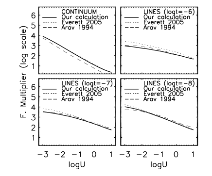
Figure A.4.— A comparison between our force multiplier calculations (solid lines) and those of Everett 2005 (dotted lines) and Arav et al. 1994 (dashed lines). The upper-left panel shows the continuum force multiplier as a function of the ionization parameter $U$. The other three panels show the line force multiplier as function of $U$ for three different values of $t$.

When the gas is highly ionized it absorbs less radiation and is subject to a weaker radiative driving force (i.e., the force multiplier is relatively small).

Figure A.4 shows the estimated force multiplier assuming a Mathews-Ferland SED. Figure A.4 has four panels, the upper-left panel represents the continuum component of the force multiplier, mainly produced by bound-bound transitions. The other three panels in Figure A.4 show the contribution to the force multiplier from bound-free transitions for three different values of the dimensionless factor $t$; ${\rm log}~{}t=$ $-6$, $-7$ and $-8$. The line force multipliers increase as $t$ decreases. This increase is noticeable when the medium is not highly ionized ($\hbox{log~{}$U$}\lesssim-1$; $\hbox{log~{}$\xi$}\lesssim 0.3$). Our calculations are in good agreement with those performed by Arav et al. (1994); Everett (2005).

Appendix F Force multipliers calculations of material illuminated by absorbed power-laws and Mathews-Ferland SED

A warm absorber shielding the outflow may increase the effectiveness of radiation driving. In this appendix we use the same unabsorbed SEDs used in §4 to estimate the amount of shielding required to significantly increase the radiative driving force. Additionally, we estimate the differences between the radiative forces produced by a soft incident spectrum and a hard incident spectrum for different ionization levels of the absorbing outflow. As in §4 we assume that the warm absorber shielding the outflow has $\hbox{log~{}($N_{\rm H}/{\rm cm}^{-2})$}=23$.

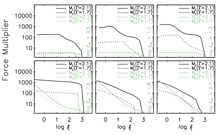
Figure A.5.— The bound-free, $M_{\rm C}$, and bound-bound, $M_{\rm L}$, components of the force multiplier are shown as a function of the ionization parameter. Force multipliers are calculated for a power-law SEDs with photon indices of $\Gamma$ = 2.1 (solid lines) and $\Gamma$ = 1.7 (dotted lines). In the upper-left, upper-right, lower-left and lower-right panel we have assumed absorbing shield where the soft and hard SEDs have been attenuated by a warm-absorber shield with $\hbox{log~{}($N_{\rm H}/{\rm cm}^{-2})$}=23$ and $\hbox{log~{}$\xi$}_{\rm sh}=$ 0.6, 1.0, 1.3, 1.6, 1.8 and 2.1 respectively.

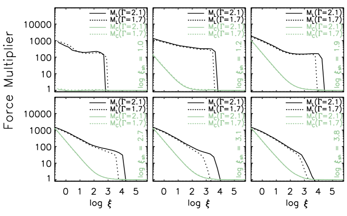
Figure A.6.— The bound-free, $M_{\rm C}$, and bound-bound, $M_{\rm L}$, components of the force multiplier are shown as a function of the ionization parameter. Force multipliers are calculated for Mathews-Ferland SEDs with X-ray photon indices of $\Gamma=2.1$ ($\hbox{$\alpha_{\rm ox}$}=-1.52$; solid lines) and $\Gamma$ = 1.7 ($\hbox{$\alpha_{\rm ox}$}=-1.41$ dotted lines). In the upper-left, upper-right, lower-left and lower-right panels we have assumed that the SEDs have been attenuated by shields with $\hbox{log~{}($N_{\rm H}/{\rm cm}^{-2})$}=23$ and $\hbox{log~{}$\xi$}_{\rm sh}=$ 1.0, 1.2, 1.9, 2.7, 3.1 and 3.8, respectively. The default parameters of a Mathews-Ferland SED are $\Gamma=1.7$ and $\hbox{$\alpha_{\rm ox}$}=-1.41$.

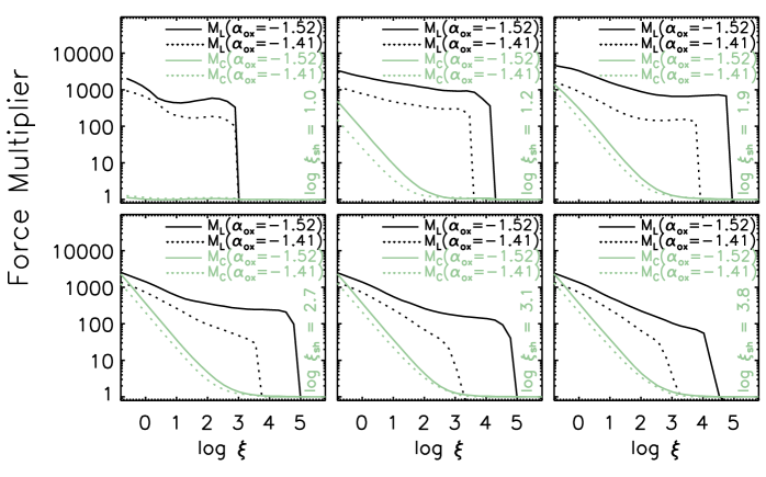
Figure A.7.— The bound-free, $M_{\rm C}$, and bound-bound, $M_{\rm L}$, components of the force multiplier are shown as a function of the ionization parameter. Force multipliers are calculated for Mathews-Ferland SEDs with X-ray photon indices of $\hbox{$\alpha_{\rm ox}$}=-1.52$ ($\Gamma$ = 1.7; solid lines) and $\hbox{$\alpha_{\rm ox}$}=-1.41$ ($\Gamma$ = 1.7; dotted lines). In the upper-left, upper-right, lower-left and lower-right panels we have assumed that the SEDs have been attenuated by absorbing shields with $\hbox{log~{}($N_{\rm H}/{\rm cm}^{-2})$}=23$ and $\hbox{log~{}$\xi$}_{\rm sh}=$ 1.0, 1.2, 1.9, 2.7, 3.1 and 3.8, respectively. The default parameters of a Mathews-Ferland SED are $\Gamma=1.7$ and $\hbox{$\alpha_{\rm ox}$}=-1.41$.

In Figure A.5 we have plotted the bound-free, $M_{C}$, and the bound-bound, $M_{L}$, components of the force multiplier as a function of the ionization parameter for soft ($\Gamma=2.1$) and hard ($\Gamma=1.7$) absorbed power-law SEDs. In the upper-left, upper-right, lower-left and lower-right panel we have assumed absorbing shields with $\hbox{log~{}($N_{\rm H}/{\rm cm}^{-2})$}=23$ and $\hbox{log~{}$\xi$}_{\rm sh}$ = 0.6, 1.0, 1.3, 1.6, 1.8 and 2.1, respectively. In Figure A.5 we show that $M_{\rm L}$ is significantly larger for incident SEDs with soft spectra (i.e., ${\Gamma=2.1}$) than for incident SEDs with hard spectra (i.e., ${\Gamma=1.7}$) especially at low ionization levels of the shielding gas. For values of $\hbox{log~{}$\xi$}_{\rm sh}\lesssim 0.6$ we do not expect strong radiative driving given the heavy attenuation of the continuum (see e.g., Chelouche & Netzer, 2003). We also note that the force multipliers $M_{C}$ and $M_{L}$ are significantly reduced for low ionization levels of the shield as shown in Figure A.5. Additionally, when $\hbox{log~{}$\xi$}_{\rm sh}\gtrsim 2.0$ the shielding becomes transparent to the radiation and therefore the force multipliers are similar to the ones in the unabsorbed case. Finally from Figure A.5 we see that when the ionization parameter of the shield lies in the range of $1.0\lesssim\hbox{log~{}$\xi$}_{\rm sh}\lesssim 1.8$ the line force multiplier of the outflowing material is greater with the presence of an absorbing shield than without one.

In Figure A.6 we have plotted $M_{C}$, and $M_{L}$ as a function of the ionization parameter for soft ($\Gamma=2.1$; $\hbox{$\alpha_{\rm ox}$}=-1.51$) and hard ($\Gamma=1.7$; $\hbox{$\alpha_{\rm ox}$}=-1.41$) absorbed Mathews-Ferland SEDs. In the upper-left, upper-right, lower-left and lower-right panels we assume shields that attenuate the SEDs with $\hbox{log~{}($N_{\rm H}/{\rm cm}^{-2})$}=23$ and $\hbox{log~{}$\xi$}_{\rm sh}$ = 1.0, 1.2, 1.9, 2.7, 3.1 and 3.8, respectively. In the case of a Mathews-Ferland SED incident on a shield with an ionization parameter in the range of $1.2\lesssim\hbox{log~{}$\xi$}_{\rm sh}\lesssim 3.8$ we find that the line force multiplier $M_{L}$ for soft SEDs (i.e., $\Gamma=2.1$) extends to larger values of the ionization parameter of the outflowing material compared to hard SEDs (i.e., $\Gamma=1.7$).

In Figure A.7 we have plotted $M_{C}$, and $M_{L}$ as a function of the ionization parameter of the outflow for soft ($\Gamma=1.7$; $\hbox{$\alpha_{\rm ox}$}=-1.51$) and hard ($\Gamma=1.7$; $\hbox{$\alpha_{\rm ox}$}=-1.41$) absorbed modified Mathews-Ferland SEDs. In the upper-left, upper-right, lower-left and lower-right panels we assume shields that attenuate the SEDs with $\hbox{log~{}($N_{\rm H}/{\rm cm}^{-2})$}=23$ and $\hbox{log~{}$\xi$}_{\rm sh}$ = 1.0, 1.2, 1.9, 2.7, 3.1 and 3.8, respectively. In the case of a modified Mathews-Ferland SED incident on a shield with an ionization parameter in the range of $1.0\lesssim\hbox{log~{}$\xi$}_{\rm sh}\lesssim 3.9$, we find that the line force multiplier $M_{L}$ is significantly larger for soft SEDs (i.e., $\hbox{$\alpha_{\rm ox}$}=-1.52$) than for hard SEDs (i.e., $\hbox{$\alpha_{\rm ox}$}=-1.41$). We note that the line force multiplier for the case of a soft Mathews-Ferland SED incident on a shield with an ionization parameter of $\hbox{log~{}$\xi$}_{\rm sh}$=1.9 has a value larger than $\sim$1000 for ionization parameters of the outflowing absorber in the range of $0\lesssim\hbox{log~{}$\xi$}\lesssim 5$. For a shield with $\hbox{log~{}$\xi$}_{\rm sh}\lesssim 1$ we predict that the continuum becomes too attenuated to allow effective radiative driving. When $\hbox{log~{}$\xi$}_{\rm sh}\gtrsim 3.1$ the shield becomes transparent to the incident radiation and therefore the force multipliers are similar to the ones estimated for the unabsorbed case (see lower right panels of Figures A.6 and A.7).

In Figure A.8 we plot the temperature of an absorbing shield as a function of its ionization parameter (on its illuminated side) for a shield with $\hbox{log~{}($N_{\rm H}/{\rm cm}^{-2})$}=23$. From the analysis in the last three paragraphs and from Figure A.8 we conclude that the most powerful winds are probably produced at temperatures in the range $4.5\lesssim{\rm log}~{}T\lesssim 5.2$. This occurs for power-law SEDs incident on shields with $1.0\lesssim\hbox{log~{}$\xi$}_{\rm sh}\lesssim 1.8$ and for Mathews-Ferland SEDs incident on shields with $1.2\lesssim\hbox{log~{}$\xi$}_{\rm sh}\lesssim 3.1$.

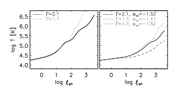
Figure A.8.— Temperature of a warm absorber (shield) as a function of its ionization parameter (illuminated side) for a warm absorber with $\hbox{log~{}($N_{\rm H}/{\rm cm}^{-2})$}=23$. In the left panel the illuminating source is a power law with $\Gamma=2.1$ (solid line) and $\Gamma=1.7$ (dotted line). In the right panel the illuminating source is a modified Mathews-Ferland SED with $\Gamma=2.1$ and $\hbox{$\alpha_{\rm ox}$}=-1.52$ (solid line), $\Gamma=1.7$ and $\hbox{$\alpha_{\rm ox}$}=-1.41$ (dotted line), and $\Gamma=1.7$ and $\hbox{$\alpha_{\rm ox}$}=-1.52$ (dashed line).

References

- Alexander et al. (2010) Alexander, D. M., Swinbank, A. M., Smail, I., McDermid, R., & Nesvadba, N. P. H 2010, MNRAS, 402, 2211.
- Arav et al. (1994) Arav, N., Li, Z.-Y., & Begelman, M. C. 1994, ApJ, 432, 62
- Bridle & Perley (1984) Bridle, A. H., & Perley, R. A. 1984, ARA&A, 22, 319.
- Chartas et al. (2002) Chartas, G., Brandt, W. N., Gallagher, S. C., & Garmire, G. P. 2002, ApJ, 579, 169.
- Chartas et al. (2007a) Chartas, G.; Brandt, W. N.; Gallagher, S. C.; Proga, D. 2007a, AJ, 133, 1849.
- Chartas et al. (2007b) Chartas, G., Eracleous, M., Dai, X., Agol, E., & Gallagher, S. 2007b, ApJ, 661, 678.
- Chartas et al. (2009a) Chartas, G., Saez, C., Brandt, W. N., Giustini, M., & Garmire, G. P. 2009a, ApJ, 706, 644.
- Chartas (2009b) Chartas, G., Kochanek, C. S., Dai, X., Poindexter, S., & Garmire, G. P. 2009b, ApJ, 693, 174.
- Chelouche & Netzer (2001) Chelouche, D., & Netzer, H. 2001, MNRAS, 326, 916.
- Chelouche & Netzer (2003) Chelouche, D., & Netzer, H. 2003, MNRAS, 344, 233.
- Dadina & Cappi (2004) Dadina, M. & Cappi, M. 2004, A&A, 413, 921.
- Dai et al. (2004) Dai, X., Chartas, G., Eracleous, M., & Garmire, G.P. 2004, ApJ, 605, 45.
- Davidson (1977) Davidson, K. 1977, ApJ, 218, 20.
- Degraf, Di Matteo & Springel (2010) Degraf, C., Di Matteo, T., & Springel, V. 2010, MNRAS, 402, 1927.
- Di Matteo (2005) Di Matteo, T., Springel, V., & Hernquist, L. 2005, Nature, 433, 604.
- Downes et al. (1999) Downes D., Neri R., Wiklind T., Wilner D.J., & Shaver P.A. 1999, ApJ 513, L1
- Egami al. (2000) Egami, E., Neugebauer, G., Soifer, B.T., Matthews, K., Ressler, M., Becklin, E. E., Murphy, T.W., Jr., & Dale, D.A. 2000, ApJ, 535, 561.
- Everett (2005) Everett, J.E. 2005, ApJ, 631, 689.
- Ferguson et al. (2001) Ferguson, J. W., Korista, Kirk. T., Verner, D. A., & Ferland, G. J., 2001, ASP Conference Series, 247, 287.
- Ferland al. (1998) Ferland, G. J., Korista, K. T., Verner, D. A., Ferguson, J. W., Kingdon, J. B.; Verner, E. M. 1998, PASP, 110, 761.
- Ferrarese & Merritt (2000) Ferrarese, L., & Merritt, D. 2000, ApJ, 539, 9.
- Fukumura et al. (2010) Fukumura, K., Kazanas, D., Contopoulos, I., & Behar, E. 2010, ApJ, 715, 636.
- Gallagher et al. (2006) Gallagher, S.C., Brandt, W.N., Chartas, G., Priddey, R., Garmire, G.P., & Sambruna, R.M. 2006, ApJ, 644, 709.
- Ganguly et al. (2007) Ganguly, R., Brotherton, M. S., Cales, S., Scoggins, B., Shang, Z., & Vestergaard, M. 2007, ApJ, 665, 990.
- Gibson et al. (2009) Gibson, R. R., Jiang, L., Brandt, W. N., Hall, P. B., Shen, Y., Wu, J., Anderson, S. F., Schneider, D. P.; Vanden Berk, D., Gallagher, S. C., Fan, X., & York, D. G. 2009, ApJ, 692, 758.
- Granato et al. (2004) Granato, G.L., De Zotti, G., Silva, L., Bressan, A., Danese, L. 2004, ApJ, 600 ,580.
- Green & Mathur (1996) Green, P.J. & Mathur, S. 1996, ApJ, 462, 637.
- Hamann et al. (2008) Hamann, F., Kaplan, K. F., Rodríguez Hidalgo, P., Prochaska, J. X., & Herbert-Fort, S. 2008, MNRAS, 391, L39.
- Hasinger et al. (2002) Hasinger, G., Schartel, N., & Komossa, S. 2002, ApJ, 573, L77.
- Hewett & Foltz (2003) Hewett, P.C. & Foltz, C.B. 2003, AJ, 125, 1784.
- Hopkins et al. (2005a) Hopkins, P. F., Hernquist, L., Cox, T. J., Di Matteo, T., Robertson, B. & Springuel, V. 2005a, ApJ, 625, L71.
- Hopkins et al. (2005b) Hopkins, P. F., Hernquist, L., Cox, T. J., Di Matteo, T., Robertson, B., & Springel, V. 2005b, ApJ, 632, 81.
- Hopkins et al. (2006) Hopkins, P. F., Hernquist, L., Cox, T. J., Di Matteo, T., Robertson, B., & Springel, V. 2006, ApJS, 163, 1.
- Jiang et al. (2007) Jiang, L., Fan, X., Ivezić, Ž., Richards, G.T., Schneider, D.P., Strauss, M.A., & Kelly, B.C. 2007, ApJ, 656, 680.
- Irwin et al. (1998) Irwin, M. J., Ibata, R. A., Lewis, G. F., & Totten, E. J. 1998, ApJ, 505, 529.
- Ivezić, et al. (2002) Ivezić, Z̆., Menou, K., Knapp, G. R., Strauss, M. A., Lupton, R. H., Vanden Berk, D. E., Richards, G. T., Tremonti, C., Weinstein, M. A., Anderson, S., Bahcall, N. A., Becker, R. H., Bernardi, M., Blanton, M., Eisenstein, D., Fan, X., Finkbeiner, D., Finlator, K., Frieman, J., Gunn, J. E., Hall, P. B., Kim, R. S. J., Kinkhabwala, Ali, Narayanan, V. K., Rockosi, C. M., Schlegel, D., Schneider, D. P., Strateva, I., SubbaRao, M., Thakar, A. R., Voges, W., White, R. L., Yanny, B., Brinkmann, J., Doi, M., Fukugita, M., Hennessy, Gregory S., Munn, J. A., Nichol, R. C., & York, D. G. 2002, AJ, 124, 2364.
- Kalberla et al. (2005) Kalberla, P.M.W., Burton, W.B., Hartmann, D., Arnal, E.M., Bajaja, E., Morras, R., & Pöppel, W. G. L. 2005, A&A, 440, 775.
- Kallman & Bautista (2001) Kallman, T., & Bautista, M. 2001, ApJS, 133, 221.
- King (2011) King, A. R. 2010, MNRAS, 402, 1516.
- Kollmeier et al. (2006) Kollmeier, J. A., Onken, C. A., Kochanek, C. S., Gould, A., Weinberg, D. H., Dietrich, M., Cool, R., Dey, A., Eisenstein, D. J., Jannuzi, B. T., Le Floc’h, E., Stern, D. 2006, ApJ, 648, 128.
- Mathews & Ferland (1987) Mathews, W. G., & Ferland, G. J. 1987, ApJ, 323, 456.
- McNamara & Nulsen (2007) McNamara, B. R., & Nulsen, P. E. J. 2007, ARA&A, 45, 117.
- Mihalas & Mihalas (1984) Mihalas, D., & Mihalas, B. W., “Foundations of radiation hydrodynamics”, New York, Oxford University Press, 1984.
- Morgan et al. (2008) Morgan, C. W., Kochanek, C. S., Dai, X., Morgan, N. D., & Falco, E. E. 2008, ApJ, 689, 755.
- Muñoz, Kochanek & Keeton (2001) Muñoz, J. A., Kochanek, C. S., Keeton, C. R.
- Murray et al. (1995) Murray, N., Chiang, J., Grossman, S. A., & Voit, G. M. 1995, ApJ, 451, 498.
- Reeves, O’Brien & Ward (2003) Reeves, J.N., O’Brien, P.T., & Ward, M.J. 2003, ApJ, 593L, 65.
- Proga et al. (2000) Proga, D., Stone, J.M., & Kallman, T.R. 2000, ApJ, 543, 686.
- Proga et al. (2004) Proga, D., Kallman, T. R. 2004, ApJ, 616, 688.
- Reeves et al. (2009) Reeves, J. N., O’Brien, P. T., Braito, V., Behar, E., Miller, L., Turner, T. J., Fabian, A. C., Kaspi, S., Mushotzky R., & Ward, M. 2009, ApJ, 701, 493.
- Riechers et al. (2009) Riechers, D. A., Walter, F., Carilli, C. L., & Lewis, G. F. 2009, ApJ, 690, 463.
- Rodriguez-Hidalgo et al. (2007) Rodriguez-Hidalgo, P., Hamann, F., Nestor, D., & Shields, J. 2007, ASPC, 373, 287.
- Rybicki & Lightman (1985) Rybicki, G. B., & Lightman, A. P. “Radiative processes in astrophysics”. John Wiley & Sons, New York, 1985.
- Saez, Chartas & Brandt (2009) Saez, C., Chartas, G., Brandt, W. N. 2009, ApJ, 697, 194.
- Schurch & Done (2007) Schurch, N. J. & Done, C. 2007, MNRAS, 381, 1413.
- Shen et al. (2008) Shen, Y., Greene, J. E., Strauss, M. A., Richards, G. T., & Schneider, D. P. 2008, ApJ, 680, 169.
- Shemmer et al. (2006) Shemmer, O., Brandt, W.N., Netzer, H., Maiolino, R., & Kaspi, S. 2006, ApJ, 646, L29.
- Shemmer et al. (2008) Shemmer, O., Brandt, W.N., Netzer, H., Maiolino, R., & Kaspi, S. 2008, ApJ, 682, 81.
- Springel et al. (2005) Springel, V., Di Matteo, T., & Hernquist, L. 2005, ApJ, 620, L79.
- Srianand & Petitjean (2000) Srianand, R. & Petitjean, P. 2000, A&A, 357, 414.
- Strateva et al. (2005) Strateva, I. V., Brandt, W. N., Schneider, D. P., Vanden Berk, D. G., & Vignali, C. 2005, AJ, 130, 387.
- Steffen et al. (2006) Steffen, A. T., Strateva, I., Brandt, W. N., Alexander, D. M., Koekemoer, A. M., Lehmer, B. D., Schneider, D. P., & Vignali, C. 2006, AJ, 131, 2826.
- Tarter, Tucker & Salpeter (1969) Tarter, C. B., Tucker, W. H., & Salpeter, E. E. 1969, ApJ, 156, 943.
- Vaughan & Uttley (2008) Vaughan S., & Uttley P. 2008, MNRAS, 390, 421.
- Wang et al. (2004) Wang, J., Watarai, K., & Mineshige, S. 2004, ApJ, 607, L107.
- Weymann et al. (1991) Weymann, R.J., Morris, S.L., Foltz, C.B., & Hewett, P.C. 1991, ApJ, 373, 23.
- Zheng & Wang (2008) Zheng, Z. Y., & Wang, J. X. 2008, ApJ, 688, 116