Constraining Type Ia Supernovae progenitors from three years of SNLS data.
Abstract
While it is generally accepted that Type Ia supernovae are the result of the explosion of a carbon-oxygen White Dwarf accreting mass in a binary system, the details of their genesis still elude us, and the nature of the binary companion is uncertain. Kasen (2010) points out that the presence of a non-degenerate companion in the progenitor system could leave an observable trace: a flux excess in the early rise portion of the lightcurve caused by the ejecta impact with the companion itself. This excess would be observable only under favorable viewing angles, and its intensity depends on the nature of the companion. We searched for the signature of a non-degenerate companion in three years of Supernova Legacy Survey data by generating synthetic lightcurves accounting for the effects of shocking and comparing true and synthetic time series with Kolmogorov-Smirnov tests. Our most constraining result comes from noting that the shocking effect is more prominent in rest-frame B than V band: we rule out a contribution from white dwarf–red giant binary systems to Type Ia supernova explosions greater than 10% at , and than 20% at level.
1. Introduction
Type Ia supernova () explosions are marvelous astrophysical tools, and they currently offer the most precise way of constraining dark energy (Sullivan et al. 2011). Today, several thousand have been observed and theoretical models and simulations are progressing rapidly (see for example Almgren et al. 2010), and many aspects of explosions can be reproduced in detail. However, these cosmic explosions, studied for decades, still are not fully understood. Particularly, we lack a solid understanding of the progenitor systems. There is consensus that arise from the thermonuclear explosion of a carbon-oxygen (C-O) white dwarf (WD), but is the WD in a binary system with a main sequence (MS) or red giant (RG) star, accreting mass from the companion to approach the Chandrasekhar limit (single degenerate –SD– scenario)? Or is the explosion caused by the merger of two WDs in a compact binary system (double degenerate –DD– scenario) ? Constraining the progenitor scenarios is key for learning the details of explosion physics, and to improve our understanding of the effects of environment on explosions and thus of the systematics that still affect the constraints on cosmology derived from SN surveys (Kessler et al. 2009; Guy et al. 2010, Wood-Vasey et al. 2007; for a review of SN Ia cosmology see Howell 2010).
No progenitor system of a has yet been observed prior to explosion: these binary systems would be very faint and undetectable, at this time, in extra-galactic surveys. Population synthesis and environment studies have not been able to firmly set constraints on the progenitors. From the theoretical point of view, generating in the DD scenario presents difficulties. The mass transfer only successfully leads to a deflagration if it occurs at a rate significantly slower than the Eddington limit, through the formation of a thick disk (Nomoto & Iben 1985), and even then fine tuning of various parameters might be needed (see Tout 2007 for a brief review, and the references therein).
Some observational evidence might already disfavor SD progenitors. While the WD accretes mass from a companion in the SD scenario, the system should emit X-ray radiation for an extended period of time. Under the assumptions of continuous duty cycle, and that all SD progenitors would emit in the X-ray, the rate is too high by over an order of magnitude compared to the number of X-ray sources observed in nearby elliptical galaxies (Gilfanov & Bogdán 2010), as well as soft X-ray sources in our own galaxy (Di Stefano 2010a). While this evidence can be used to set upper limits to SD progenitors, Di Stefano (2010b) points out that there are too few super soft X-ray sources, sources with energy typically 10 to and luminosity to , to account for the Type Ia rate within the DD scenario as well, suggesting instead that super soft X-ray radiation may not always be emitted in nuclear-burning white dwarf systems and that it could be absorbed within the system itself. A few peculiar have been observed in the past few years to produce masses close to, or in excess of, the theoretical limit for a WD mass: the Chandrasekhar limit. These apparent super-Chandrasekhar may originate from the merger of two WDs, in the DD scenario (Howell et al. 2006; Silverman et al. 2011; Yuan et al. 2010).
Kasen (2010) – hereinafter K10 – explores the effect that a non-degenerate companion star would have on the observables of the explosion, and shows that in the SD scenario, the presence of a companion may manifest itself in the early days after the SN explosion as a flux excess. As the cloud of SN ejecta expands, it collides with the companion. This impact shocks the expanding material creating a hole in the otherwise optically thick ejecta shell through which radiation can escape. An excess flux is produced in the shocked gas, propagating in the direction of the observer, and it should be detectable when the geometry is favorable and the observer looks into the companion star. As the the equilibrium temperature of the shocked debris is inversely proportional to the distance from the WD center to the power of 3/4 (see Eq. 7 in K10), the flux excess is larger the larger the separation from the companion, and assuming Roche lobe overflow, RG companions will leave the most prominent signature. The intensity of the feature is higher in bluer bands (see Section 3). The effect only lasts a few days, completely vanishing by 10 days after explosion.
With detailed early time lightcurves we may be able to identify the progenitor system of a particular SN explosion, singling out events generated by red giant progenitors when seen from favorable angles. Unfortunately, early detailed SN lightcurves, with daily or so cadence, are still rare. New surveys like the PanSTARRS Medium Deep Survey (PS1, Pastorello et al. 2010) and the Palomar Transient Factory (PTF, Law et al. 2009) provide well sampled early lightcurves, which might lead to the identification of progenitors in individual cases, as might early UV follow up.
With the large collection of lightcurves provided by surveys such as the Supernova Legacy Survey (SNLS, Astier et al. 2006) and the Sloan Digital Sky Survey (SDSS, Abazajian et al. 2009) the companion scenarios can be constrained in a statistical fashion. The SDSS collaboration recently searched for evidence of an early flux excess due to shocking in high signal-to-noise ratio (S/N) spectroscopically confirmed lightcurves from the SDSS-II survey. Finding no evidence of shocking-related excess in a subset of 108 confirmed with well observed early time behavior, Hayden et al. 2010a conclude that RG’s cannot be the main channel for explosions. Here we use confirmed from the first three years of SNLS data to set an upper limit to the contribution of RGs to progenitors.
After describing the dataset used here, consisting of spectroscopically confirmed from the first three years of SNLS, and the processes used to standardize the data and generate composite lightcurves (Section 2), in Section 3 we summarize the results presented in K10 and show our rendering of these models. We then describe the statistical tests that allowed us to derive constraints to the contribution from RG progenitors to explosions (Section 4). We also extended our analysis beyond the spectroscopically confirmed sample to include photometrically selected lightcurves, showing that lightcurves affected by shock were not rejected as spectroscopic follow up candidates in SNLS because of a selection bias, and that our conclusions extend to the photometrically selected (Section 5). Finally, in Section 7 we summarize our conclusions and outline future work.
2. SNLS data, third year
The dataset used here is described in detail in Conley et al. (2011), Guy et al. (2010), González-Gaitán et al. (2011) and Bazin et al. (2011). We use data from the first 3 years of the SNLS. The SNLS is a rolling survey that gathered photometric data at the Canada-France-Hawaii-Telescope (CFHT). Two independent photometric pipelines, based in France and Canada, are used for the SNLS data reduction (Bazin et al. 2011; Perrett et al. 2010). Here we use the photometry output of the French pipeline. SNLS lightcurves, originally collected in griz (Regnault et al. 2009b), are k-corrected (Hsiao et al. 2007), and standardized by applying a stretch factor, to broaden or narrow the rest-frame timescale of the lightcurve (Perlmutter et al. 1997), in order to generate rest-frame and band lightcurves111Note that this is different from what is done in the processing of SNIa lightcurves for cosmology, where the stretch correction is applied to the rest-frame template, to match the data (Conley et al. 2011; Sullivan et al. 2011).. We define the variable as
| (1) |
where is the date of maximum flux (in rest-frame filter band), is the SN redshift and the stretch; represents the rest-frame, stretch-corrected, time to peak luminosity. We processed the lightcurves using the SiFTO method (Conley et al. 2008) and we used a single template to fit the data and stretch correct the lightcurves. In processing the SN data we assumed a rise time days, the time elapsed between explosion and maximum B luminosity, according to what González-Gaitán et al. (2011) finds in a similar (but larger) SNLS dataset, and it is also consistent with the rise time derived in Hayden et al. (2010b) from SDSS-II ().
Our primary analysis is focused on spectroscopically confirmed . The first 3 years of SNLS data offer over 200 spectroscopically confirmed lightcurves. The original dataset was reduced to 87 SN lightcurves by applying quality and redshift cuts described below. The final dataset uses only SNe that satisfy the following requirements:
-
•
spectroscopically confirmed Type Ia SNe at redshift (135 lightcurves)
-
•
the total reduced for the SiFTO template fit, applied to epochs days, is better than 3.0 (130 lightcurves)
-
•
the error in the determination of the peak date is days (117 lightcurves)
-
•
have at least three data points in rest-frame and three data points in rest-frame band in the rise portion of the lightcurve, days, to ensure the quality of the pre-peak fit (87 lightcurves).
The excess due to shocking may be visible up to 10 days after explosion (K10), or given our choice of days. No data prior to days were used to standardize the data and generate our composite lightcurves in order to avoid including in the lightcurve fitting process data points potentially affected by the excess that we are seeking. Different choices of minimum day (between -10 and -7) were also tested and they do not affect our result. However removing points earlier than causes, in a few cases, a poor lightcurve fit, and thus a larger scatter in the data. Visual inspection reveals that none of those for which the fit parameters significantly change if data points between and are excluded is actually affected by shocking. Thus we conclude that including points at only strengthens the significance of our results.
The templates adopted to process the data (Conley09c and Conley09f222We see no difference in our results choosing either Conley09c or Conley09f, and where not specified we will refer to Conley09f throughout the paper., Conley et al. 2008) assume a parabolic behavior in time prior to days333In fact, the SiFTO method allows as well for a cubic fit to the early rise portion of the lightcurves, but this was found not to improve the lightcurve fit in most cases (Conley et al. 2008)., as described in Goldhaber et al. (2001), Conley et al. (2008), and in the references therein :
| (2) |
where is the flux as a function of time , and rise time . This is consistent with a simple expanding fire ball modeling of the exploding ejecta (see for example Riess et al. 1999), with representing the rise “speed,” which is what we expect in absence of shocking by a companion. We refer the reader to González-Gaitán et al. (2011) for a detailed study of the rise behavior of in the SNLS data.
Hayden et al. (2010b) found that a better fit to the SDSS-II data can be achieved using two separate templates to fit the rise and fall portion of the lightcurves, thus obtaining two stretch values. While using 2 stretches slightly improves the per degree of freedom the individual lightcurve fits, F-tests show that for these SNLS data the improvement achieved using 2 stretches is not significant (see also González-Gaitán et al. 2011). Furthermore, because we use only data points at , with the 5 day cadence of the SNLS data, we generally have only 2-3 points in the rise portion of each lightcurve that would be used for fitting. Fitting separately the rise and fall portions of the lightcurve then exposes us to the risk of misfitting or over-fitting the rise portion. We conclude it is best to use a single stretch template for the purpose of this analysis.
A more detailed description of the standard SNLS lightcurve processing can be found in Conley et al. (2011), Guy et al. (2010), and Conley et al. (2006). For a discussion on the SNLS photometric calibration see Regnault et al. (2009a).
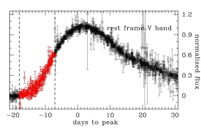
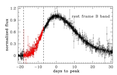
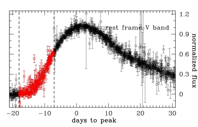
The SNLS lightcurves, normalized to peak flux in each color channel, stretched, and k-corrected as described above, can be combined into a composite lightcurve: our composite rest-frame (V) lightcurve contains a total of 1059 (1125) data points between and , and 202 (217) in the 10 days after explosion that would be affected by the flux excess: days. The composite and lightcurves are shown in Figure 1, band flux on the left hand side and band flux on the right hand side444For a discussion on the distinction between photon-based, and energy-based flux see Nugent et al. (2002). Throughout the paper we refer to flux as photon-based flux.. The data points potentially affected by the shocking excess are plotted in red, and included within vertical lines.

3. Models
After an explosion, the SN ejecta expands and collides with the companion star, if one exists. K10 showed that this impact shocks the SN ejecta creating a hole in the expanding material. Radiation can now escape from the otherwise optically thick ejecta shell. An early X-ray emission, analogous to the X-ray flash in core-collapse SN (Soderberg et al. 2008; Modjaz et al. 2009), should last minutes to hours, with little chance to be observed. In UV and optical bands the flux excess lasts longer: the gas begins expanding to refill the hole carved by the companion. Radiation continues to diffuse out of this hot, shocked region, and it is observable until the luminosity begins to dominate the lightcurve. The time scale for this process is roughly 5-10 days. The effect is more prominent in bluer bands and can span over an order of magnitude in flux in UV, generating an early peak even brighter than the peak luminosity in absence of shocking, while it is substantially dimmed in V band.
The size of the hole and of the shocked gas region, and thus the amount of radiation escaping, depend essentially on the solid angle subtended by the companion carving the hole, and on velocity of the ejecta at the time of impact. The models assume that the companion star is in Roche lobe overflow and that the exploding WD has reached the Chandrasekhar limit. Under such assumptions these are determined by the distance to the companion, and the geometry of the system (semi-major axis of the binary orbit and size of the Roche lobe) is set by the nature of the companion. This excess radiation is then a powerful tool to identify the SN progenitor system.
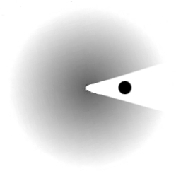
K10 considered 3 types of companions: a MS star, at a distance from the WD, a MS companion at , and a RG companion at . The effect is most prominent for observers viewing directly into, or at small angles from, the companion (i.e. into the hole), or roughly of the time (Figure 2). However, particularly in the case of RG companions, where the excess is maximum, some flux excess is observable even at large angles. We expect the distribution of viewing angles to be uniform in nature, and in our set of lightcurves. The presence of a flux excess may increase the detectability of a SN, thus the orientation of the WD-companion system may constitute a selection bias when operating close to a survey detection limit. The cut at assures that we keep safely away from the detection limit of SNLS. Furthermore the maximum excess in B band is significantly smaller (a factor ) than the peak luminosity, and since SNLS is a rolling survey, covering each field every five days, each lightcurve should, in principle, contain data points within 10 days of peak that would be brighter than the maximum shocking flux. The shock-induced flux excess, therefore, does not significantly increase the detectability of a SN in our sample, and we can assume that the distribution of angles in our data is unbiased. Later we will expand our analysis to a photometrically selected sample, to assess weather an early flux excess might have caused the to be misclassified as a non-, and thus not followed spectroscopically (Section 5).
The models are generated from 2-dimensional Monte Carlo radiation transport simulations that are subject to random sampling errors. Such errors are purely statistical, and don’t take into account any of the possible systematic errors or uncertainties in the model calculations. The statistical errors are accounted for throughout our analysis.


The excess generated by shocking is shown in Figure 3, averaged over viewing angles, for all three progenitor scenarios in both B and V band.
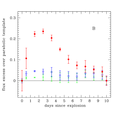
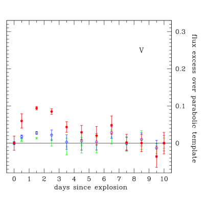
It is evident that, while the RG progenitors generate a significant excess, and a very distinct effect in both B and V band, the time behavior for MS stars is only marginally changed in the presence of shocking, especially after averaging over viewing angles. Such a small deviation from the parabolic early rise behavior would hardly be detectable in the presence of the typical noise of SNLS data. Therefore we restrict ourselves to the RG scenario and only try to constrain the RG contribution to SN progenitor systems. We also expect that the explosion in a DD scenario would show even smaller, or no, deviations from a parabolic behavior. We thus tentatively associate the DD scenario to the standard template. Note, however, that it is possible, as mentioned in K10 and shown in Fryer et al. (2010), that in a WD merger gas would be blown out to large radii (), producing a shock signature, with a UV excess possibly propagating through visible wavelengths. However, the simulations in Fryer et al. (2010) generally produce lightcurves rather dissimilar from standard , with broader visible band lightcurve, unlikely to match in our sample.
Where needed, we will assume that any explosion not generated by a RG-WD binary pair has equal probability of arising from any of the three remaining scenarios.
3.1. Rendering of the models
The K10 simulations generate full spectra of the SN explosion, including the effects of shocking, at time intervals of 0.1 days for the first 10 days after explosion. The spectra are integrated on a day time scale and filtered through the same V and B filters into which the SNLS data have been converted. This is done for every angular separation between the WD and the companion, in 40 equal intervals of observing probability, for the three progenitor scenarios considered: RG, and MS sub-giants.
The K10 spectra are designed to reproduce the excess generated by shocking on top of a nominal template. The input template in the models is irrelevant to the shocking physics. We use the spectra for the smallest companion scenario () at the largest angular separation (), where we expect the effects of shocking to be entirely negligible, as a neutral template: the template in absence of shocking. To better reproduce what we actually expect the result of shocking to look like in a SNLS lightcurve we subtract the neutral template from the lightcurve templates generated as described above. The new lightcurves are shown in Figure 3, averaged over all angles, and they describe the excess due to shocking. This excess can be added to the parabolic portion of the templates to reproduce what we would expect to see in our data. The reader is reminded that this portion of the lightcurve is not used to standardize the SNLS data and generate the composite lightcurves.
We now have template lightcurves for the first 10 days of a explosion in the SD scenario, with different companion stars and at different observing angles, which can be compared to the SNLS observations.
4. Tests
4.1. Template goodness of fit
We begin by noticing that the fit of the composite SN to the SN template (here Conley09c and Conley09f were used, with no significant differences) is worst in the region of interest for the shocking effect, days to peak, in both and bands.
]


Figure 4 shows the median, binned by day, of the composite lightcurves (top plots). The error bars represent the scatter – standard deviation – of the individual measurements (the standard deviation is measured as conventionally done with respect to the mean and we ignore the error of each measurement). The bottom plots show the deviation from the template as the difference between the data, , and in the template, , at time , over the error in the data , averaged over each day:
| (3) |
as an estimator of the goodness of fit of the template to the composite lightcurve. The propagation of errors along the time dimension is also ignored.
The most significant deviation from the template happens in both and band roughly prior to days, with a clear excess in band at or in the first few days after explosion. It is intriguing that the deviation is more prominent in than in band, consistent with the chromatically biased effect that shocking by a companion would produce. Note, however, that this is the portion of the lightcurve that is not fit to the template, and it is thus not surprising to see a larger scatter here.
4.2. Simulations
Having found a deviation from our fiducial template in the early days after explosion, we test if this can be attributed to shocking by a companion.
With the K10 templates in hand we can create synthetic rise lightcurves that incorporate the effect of shocking for the different progenitor scenarios, as seen from different viewing angle. We start off with the standard parabolic rise templates (Conley09f). In each band we add the excess described by the models (Figure 3) to our standard template. For each epoch corresponding to the SNLS data, we draw a data point from the new template thus obtained. To choose the viewing angle from which this data point should come we draw angles with equal probability between 0 and 180∘.
Families of synthetic lightcurves are generated using increasing contributions of data points from the RG progenitor scenario, and drawing the remaining points equally likely from a parabolic template (DD scenario), the and the MS progenitor scenarios. We generate families with 0% RG contribution, to 100% RG contribution, in steps of 10%. A finer grid was also tested, but a resolution of 10% in the RG contribution is adequate to represent the progenitor populations given our errors.
In our test we have to account for the errors in both the templates and the data. Thus at a given epoch, in generating the simulated data points, we draw each flux value from a Gaussian distribution around the template value at the corresponding epoch, where the width of the Gaussian is the sum in quadrature of the errors in the SNLS data and in the model.
For each between and 100% we create 100 sets of simulated observations, in steps of 10%, thus generating 100 synthetic lightcurves per , each one the size of the rise portion of the lightcurve: 202 points in B and 217 in V band.
4.3. One band K-S test
We then compare each population of synthetic lightcurves to our composite lightcurves. We chose the non-parametric 2-sample Kolmogorov-Smirnov (K-S) test (Peacock 1983) to do so. This simple statistical test measures the maximum distance between the simulated and true cumulative lightcurves, and we find it is a sensible statistic to determine the presence of an excess in data with large scatter. The K-S tests are non parametric, and thus do not require us to make any assumptions on the distribution of data, and, unlike for example the Pearson’s statistics (Rice 2001), do not require binning the data. The SNLS data points are sorted by flux, and added to generate a cumulative flux distribution. Similarly, a cumulative flux distribution is generated for each synthetic realization. The maximum distance between two cumulative distributions is a measure of the level at which the null hypothesis that the data sets being compared come from the same distribution, can be rejected (see Figure 5). In other words: comparing the true data with synthetic data generated from scenarios with different RG contributions, we test if the data comes from a distribution with a given fraction of RG progenitors, .

For each , we pair each of the 100 sets of simulated observations with our true lightcurve, apply a 2-sample K-S tests, and average over the 100 K-S numbers. This allows us to obtain the confidence level for the rejection of the null hypothesis – that the two sets being compared come from the same distribution – and its statistical errors, accounting for all sources of noise: the uncertainty in the models, in the data, and for the presumed diversity in progenitors.
Using only the data, and within error bars, we reject at roughly 90% confidence level (c.l.) the hypothesis that a progenitor population with has generated our data. A contribution of more than is ruled out at the c.l. These results are largely consistent with the analysis presented in Hayden et al. (2010a), and with the upper limits placed by (Gilfanov & Bogdán 2010) in SNIa in elliptical galaxies. Accounting for all angles, with only data points in the 10 days that would be affected by the shocking effect, we would expect data points to be affected significantly by the effect we are probing, even if all companions were RGs. This is therefore a small number statistics problem, in the presence of noise in both data and models, and it is not surprising that we have a limited ability to place strict limits to the contribution of RG progenitors this way. However we will obtain stronger limits by including considerations on the color bias in the shocking excess in the next section (Section 4.4).
Noticeably, despite the noise, the probability that the true and synthetic distribution of data points come from the same progenitor distribution clearly decreases monotonically as we increase the contribution of RG systems, particularly in the band (Figure 6). This strongly suggests a minimal contribution of RGs to progenitors. Similarly, an almost monotonic decrease in probability (increase in c.l.) is evident in the band, though less pronounced. This is expected, on account of a smaller signature of shocking in redder bands (see Figure 2).
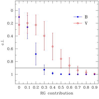
4.4. K-S chromatic test
In this section we investigate the chromatic bias in the shocking footprint. In absence of shocking, the expected time behavior of the SN explosion is a parabola, similar in and band. Thus, in the rise portion of the lightcurves we would expect points drawn from a set of SNe to come, statistically speaking, from the same distribution in and band. However, in the K10 simulations (see Section 3) the and time behavior differ dramatically in the rise portion of the lightcurve in the presence of RG progenitors. We again perform a 2-sample K-S test. This time we want to asses the similarity of the B and V populations of early-rise data, so for the SNLS data and we compare the B and V channel with a K-S test, and we do the same for each synthetic population.
We find that the hypothesis that rest-frame and populations of data points from the composite true SNLS lightcurves, day 0-10 after explosion, come statistically from the same distribution can only be rejected to c.l., or equivalently that the hypothesis that the two channels come from the same distribution has a .
We compare the synthetic B and V lightcurves, and find, as expected, that the K-S number increases with the increasing RG contribution: the probability that the B and V synthetic data come from the same distribution decreases as more RG progenitors are used in the progenitor mix.
The results of this test are plotted in Figure 7. Within error bars, only the population with no contribution from RG progenitors is consistent with the SNLS data. We rule out a contribution at , and greater than 20% at level.

4.5. Color distributions


In standardizing our lightcurves we have chosen one stretch value for each lightcurve to be applied to all rest-frame bands. We ask the question: could there be a correlation between and that would interfere with the result of our K-S chromatic test (see Section 4.4). Suppose some data points in the region days, which is not fit to the template, have more (or less) flux than the template, so that if we included those points when fitting the lightcurve to the template we would have generated different fit parameters, and a different value for the stretch or day of maximum; in this case both the and lightcurves would show flux in excess (deficit) of the template in the shock region. We might then see a correlation in our and composite lightcurves. Any such correlation would systematically lower the K-S number (higher the for the null hypothesis) found for the true data. Meanwhile our simulated lightcurves are generated independently in B and V bands. Since in our chromatic K-S test even the simulations which use no RGs among the progenitors are consistent with our true data at the level, but show a lower , indicating a greater discrepancy between B and V band, we further explore this possibility, seeking an independent confirmation of what we see in the K-S tests beyond this possible systematic correlation.
We test the color of our true and simulated lightcurves by taking to be the difference of the B and V flux after normalizing each channel at peak. Under the assumption that in absence of shocking the rise portion of the lightcurve would follow a parabolic behavior identical in both bands, diverging only at as modeled in the Conley09f template, the distribution of values should be consistent with 0 for our composite lightcurves, while the effect of shocking would produce a distribution of with a positive mean, and a large standard deviation.
For every flux point in each normalized, standardized rest-frame lightcurve, we subtract the flux of the closest rest-frame data point, within . Similarly, we generated synthetic colors for different RG fractions, by creating pairs of V and B synthetic lightcurves, accounting as usual for the typical error bars in the data and in the models. We derive the distribution of colors for both true and simulated data.
The distributions are plotted in Figure 8. The top panel shows the distribution for true data. There is no blue excess in flux in the true color: in fact the distribution has a mean of , a median , and a standard deviation : statistically consistent with a random distribution around 0.
The distributions generated from simulated lightcurves are shown below the distribution for true data in Figure 8, for RG contributions , plotted from the top to the bottom. Each distribution is generated from a factor of 100 more points than the true color distribution and is thus minimally noisy. The mean of the distribution increases as we increase and the distributions get increasingly asymmetric, weighted toward positive values of (bluer color). The synthetic distributions generated with no RGs (=0%) has moments that are extremely similar to those of the true color distribution: , median and . Once again, this shows that the distribution of colors in the SNLS data is compatible with minimal – or no – contribution of RG to progenitors, confirming the results obtained from the K-S tests.
5. Photometrically selected
The excess due to shocking of the SN ejecta affects the early time domain photometric and spectral behavior of the explosions. Since in surveys such as SNLS and SDSS are identified by their early lightcurves, and thus an explosion is followed up spectroscopically only if it is thought to be a SN explosion, an interesting question is whether this early effect might have lead to the rejection of phenomena that indeed were , but deviated from the expected early behavior on account of shocking. In Hayden et al. (2010a), a subset of unconfirmed is visually inspected and no such effect is found. We investigate 905 SNLS lightcurves with some redshift information, either spectroscopic or photometric. We exclude likely or known AGN, variable stars, and core-collapse (CC) SNe. In order to avoid contamination from unidentified SNe II, Ib, or Ic, we also apply cuts in stretch and color space. In particular, CC SNe show a different average color than SNe Ia, and color constraints eliminate them from the sample. A detailed discussion of photometric selection of in the SNLS data can be found in Bazin et al. (2011). We thus believe our new dataset has minimal contamination from non events. Our new dataset contains 336 lightcurves before our cuts are applied (see Section 2), and 110 after. Our new composite lightcurves contain 251 points in rest-frame and 270 in rest-frame in the region of interest: =-17.4 to -7.4 days to peak (Figure 9).
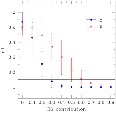
We repeat the K-S tests applied earlier to the extended set and find that the statistics confirm the upper limits set to the contribution of RG binary systems to explosions (Figures 10 and 11). The K-S test of the composite lightcurve in each B and V with the respective synthetic lightcurves is entirely consistent with the test for the spectroscopically confirmed subset, and consistent with minimal or no contribution of RG to the progenitors.

6. U band data
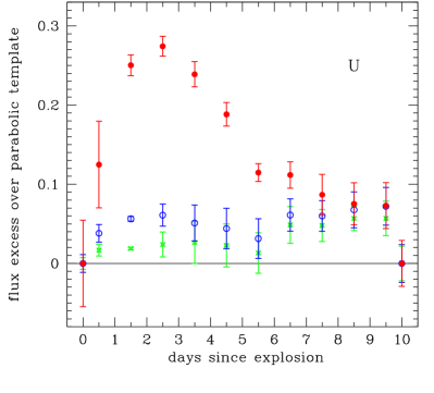
As described in Section 3, the excess due to shocking is more prominent at bluer wavelengths. In band, the models by K10 predict an excess over a nominal template more pronounced by roughly 20% over the B band for the RG case, averaged over all angles and over the first 10 days after explosion. The prediction for the angle averaged excess in band is shown in Figure 12. We thus extend our analysis to the rest-frame band data, to see if a stronger constraint can be placed to the contribution of RG to the progenitor population.
.
Three years of SNLS spectroscopically confirmed lightcurves are processed as described in Section 2, in order to generate rest-frame band lightcurves. The lightcurves are then selected if they pass similar cuts to those described earlier:
-
•
spectroscopically confirmed Type Ia SNe at redshift (135 lightcurves)
-
•
the total reduced for the SiFTO template fit, applied to epochs days, is better than 3.0 (130 lightcurves)
-
•
the error in the determination of the peak date is days (117 lightcurves)
-
•
have at least three data points in rest-frame B, three data points in rest-frame V, and three in rest-frame band in the rise portion of the lightcurve, days, to ensure the quality of the pre-peak fit (57 lightcurves).
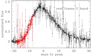
The rest-frame band composite lightcurve thus generated is plotted in Figure 13, and it contains 662 points between days -20 and 40 from explosion, and 123 in the region of interest: . Applying the latter cut, which is more restrictive than the corresponding cut in our primary analysis, the new composite and lightcurves contain, respectively, 152 and 161 data points in the region . It is immediately evident that the band composite lightcurve is significantly noisier than the and composites, and it contains 35% fewer lightcurves, and roughly 40% fewer relevant data points.
We generate synthetic band lightcurves as described in Section 4.2 and we reproduce the 2-sample, monochromatic K-S test we described in Section 4.3 for the band data. We find that the true data distribution once again grows dissimilar from the simulated distribution as more RG progenitors are included in the simulation (Figure 14). Using the data a progenitor fraction is ruled out at the level. The results of the single band K-S test for the and for the subsample of lightcurves that pass the new set of cuts are also plotted, and they are entirely consistent, though with larger errors on account of the smaller dataset size, with the results obtained in Section 4.3.
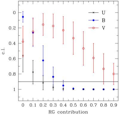
Note that the band data, even in absence of RG in the simulated data, appears from a K-S test to be different at the level from the parabolic-rise model (i.e. the 2 limit of the c.l. of rejection of the null hypothesis that synthetic and true data come from the same distribution is below c.l. = 0 for all synthesized populations). The simulated lightcurves are generated as described in Section 4.2, and an adiabatic (parabolic) expansion is postulated up to 6 days after explosion. However, effects of line opacity and dispersion in the spectra at wavelengths bluer of , as described in Ellis et al. (2008), affect the lightcurve, and may modify it from the our simple model prediction. This can explain the relative low correlation between our true and simulated data, which is revealed by the K-S test. For this reason we are reluctant to apply the chromatic K-S test describe in 4.5 to the U band data, as our assumption that the U and B, or U and V lightcurves would have identical early rise behavior might not hold here. As a matter of visualization though, we reproduce Figure 8 for the and data (see Section 4.5). As in all other cases considered, the distribution of simulated color gets increasingly different from the distribution of true data as we increase the contribution of RG in the progenitor mix for our simulations.


We limit ourselves to point out that the band data confirms the constraints that we set with and data.
7. Conclusions
We analyzed 3 years of spectroscopically confirmed from the SNLS survey looking for an early rise flux excess that could be attributed to shocking by a companion. We created composite lightcurve standardizing the data with the SiFTO method, excluding from the fit the region that might be affected by the shocking phenomenon.
We found a worsening of the fit of the data to the standard templates in the first few days after explosion (Section 4.1), but we found no evidence that is due to anything but the fact that the data prior to are not used in the template fit.
We used the spectra generated by the K10 (Kasen 2010) simulations to model the expected time domain behavior in the SD scenario, thus we can account for sources of noise in the models, as well as in the data. We found no evidence of flux excess in our data, and conclude that, based on the K10 models, the contribution from RG progenitors is less than 10% in the SNLS 3-year sample. We thus set a upper limit of 10% to the contribution of RG-WD binary systems to the progenitors, and a upper limit of 20%. With roughly 100 lightcurves in our sample, with a contribution of lightcurves from RG progenitors, data points could be affected by shocking. We cannot exclude such a small contribution from RG binary systems in the presence of noise from both the models and the data. Our results are robust when tested in a photometrically selected sample of lightcurves, as well as using band data.
Our conclusion agrees with the results derived in Hayden et al. (2010a) from the SDSS-II sample. Our analysis differs, other than in the SN sample used, in the treatment of the shocking signature: while Hayden et al. (2010a) models the shocking as a Gaussian excess we used the K10 simulation directly to characterize effects of shocking, thus including the uncertainties in the models. Furthermore, our analysis exploited the color bias in the shocking excess to set stronger constraints on the presence of shocking and are able to quantify the maximum allowed contribution of RGs to the progenitors.
Although Bayesian tests (Expectation Minimization and Gibbs sampling) were applied to our data, the presence of noise, and the relatively high dimensionality of the problem, with four possible progenitor scenarios, does not allow us to firmly asses what contribution of RGs best reproduces the residuals we see in the data with respect to the parabolic templates. Our data is entirely consistent with no RG progenitors.
According to population synthesis studies, such as for example Ruiter et al. (2009), the SD scenario is expected to produce mainly from evolved companions, i.e. they favor the RG-WD channel over the MS-WD channel, at least under the Roche lobe overflow requirement. In Ruiter et al. (2009), where reaching the Chandrasekhar limit is required, as it is assumed in this paper and in the K10 simulations, MS-WD binaries are responsible only for 5% to 10% of the production, while the majority of come from a system with an evolved donor: a sub-giant, or giant. Limiting the contribution of RG-WD progenitors from an observational point of view may then have a significant impact on the conclusions derived from population synthesis stidies on delay time distributions and progenitors.
The PanSTARRS Medium Deep Survey (PS1, Pastorello et al. 2010) and the Palomar Transient Factory (PTF, Law et al. 2009) have begun providing well-sampled rise lightcurves, where the excess due to shocking by a RG progenitor, should this be a valuable channel to produce , could soon be observed. Since the effect is predicted to be chromatically biased (see Section 3), PS1 is particularly suitable, offering data in SDSS g and r bands, thus allowing a color comparison. Early UV follow up surveys (Cooke et al. 2011) are also a promising way to spot WD-RG progenitor systems, since the progenitor excess is extremely prominent in UV bands, provided that the follow up can be triggered early enough after explosion. SNLS continued collecting time series through 2006 and as all SNLS data become available more stringent limits may be set. Note that in absence of any excess the population of progenitors could be pinpointed to small () progenitor companions. However, in the presence of detections of small excess signals there would be a degeneracy between RG progenitors observed at some angular offset from the line of sight to the hole generated by the companion, and more massive MS companions, and a large sample is indeed necessary to disentangle these two scenarios. Possibly, only a survey as large as LSST (LSST Science Collaboratio 2009) would offer the opportunity to asses the frequency of progenitor companion types in .
We also point out that the constraints derived here rely on the theoretical models described in K10. The shocking signatures predicted in K10 assume the companion is in Roche lobe overflow, with the separation distance, , only a few times the stellar radius, . While this is expected in a typical accretion scenario, if the solid angle subtended by the companion would be smaller, and so would be the effect of shocking. Justham (2011), for example, argues that the donor star in the SD scenario might shrink rapidly before explosion, having exhausted its envelope; the companion star would then be many times smaller then its Roche lobe, reducing the shocking signature, and also explaining the lack of hydrogen in spectra of . We look forward to more detailed theoretical work, which may relax the Roche lobe overflow assumption, integrate three dimensional explosion models, and takes into account possible absorption mechanisms within the systems, and the effects of the orbital motion, to better characterize the shocking behavior and its diversity.
The authors wish to thank Lars Bildsten (KITP) and Ryan Foley (CfA) for stimulating discussions and insightful comments.
The SNLS collaboration gratefully acknowledges the assistance of Pierre Martin and the CFHT Queued Service Observations team. Jean-Charles Cuillandre and Kanoa Withington were also indispensable in making possible real-time data reduction at CFHT. This paper is based in part on observations obtained with MegaPrime/MegaCam, a joint project of CFHT and CEA/DAPNIA, at the Canada-France-Hawaii Telescope (CFHT) which is operated by the National Research Council (NRC) of Canada, the Institut National des Sciences de l’Univers of the Centre National de la Recherche Scientifique (CNRS) of France, and the University of Hawaii. This work is based in part on data products produced at the Canadian Astronomy Data Centre as part of the CFHT Legacy Survey, a collaborative project of NRC and CNRS. MS acknowledges support from the Royal Society. Canadian collaboration members acknowledge support from NSERC and CIAR; French collaboration members from CNRS/IN2P3, CNRS/INSU and CEA. Based in part on observations obtained at the Gemini Observatory, which is operated by the Association of Universities for Research in Astronomy, Inc., under a cooperative agreement with the NSF on behalf of the Gemini partnership: the National Science Foundation (United States), the Science and Technology Facilities Council (United Kingdom), the National Research Council (Canada), CONICYT (Chile), the Australian Research Council (Australia), CNPq (Brazil) and CONICET (Argentina). Based on data from Gemini program IDs: GS-2003B-Q-8, GN-2003B-Q-9, GS-2004A-Q-11, GN-2004A-Q-19, GS-2004B-Q-31, GN-2004B-Q-16, GS-2005A-Q-11, GN-2005A-Q-11, GS-2005B-Q-6, GN-2005B-Q- 7, GN-2006A-Q-7, and GN-2006B-Q-10. Based in part on observations made with ESO Telescopes at the Paranal Observatory under program IDs 171.A-0486 and 176.A-0589. Some of the data presented herein were obtained at the W.M. Keck Observatory, which is operated as a scientific partnership among the California Institute of Technology, the University of California and the National Aeronautics and Space Administration. The Observatory was made possible by the generous financial support of the W.M. Keck Foundation.
Facilities: CFHT, VLT:Antu, VLT:Kueyen, Gemini:Gillett, Gemini:South, Keck:I.
References
- Abazajian et al. (2009) Abazajian, K. N., et al. 2009, ApJS, 182, 543
- Almgren et al. (2010) Almgren, A., et al. 2010, ArXiv e-prints
- Astier et al. (2006) Astier, P., et al. 2006, A&A, 447, 31
- Bazin et al. (2011) Bazin, et al. 2011, in preparation
- Conley et al. (2011) Conley, A., et al. 2011, ApJS, 192, 1
- Conley et al. (2006) Conley, A., et al. 2006, AJ, 132, 1707
- Conley et al. (2008) Conley, A., et al. 2008, ApJ, 681, 482
- Cooke et al. (2011) Cooke, J., et al. 2011, ApJ, 727, L35
- Di Stefano (2010a) Di Stefano, R. 2010a, ApJ, 712, 728
- Di Stefano (2010b) Di Stefano, R. 2010b, ApJ, 719, 474
- Ellis et al. (2008) Ellis, R. S., et al. 2008, ApJ, 674, 516
- Fryer et al. (2010) Fryer, C. L., et al. 2010, ApJ, 725, 296
- Gilfanov & Bogdán (2010) Gilfanov, M., & Bogdán, Á. 2010, Nature, 463, 924
- Goldhaber et al. (2001) Goldhaber, G., et al. 2001, ApJ, 558, 359
- González-Gaitán et al. (2011) González-Gaitán, S., et al. 2011, in preparation
- Guy et al. (2010) Guy, J., et al. 2010, A&A, 523, A7
- Hayden et al. (2010a) Hayden, B. T., et al. 2010a, ApJ, 722, 1691
- Hayden et al. (2010b) Hayden, B. T., et al. 2010b, ApJ, 712, 350
- Howell (2010) Howell, D. A. 2010, Nature Communications, accepted
- Howell et al. (2006) Howell, D. A., et al. 2006, Nature, 443, 308
- Hsiao et al. (2007) Hsiao, E. Y., Conley, A., Howell, D. A., Sullivan, M., Pritchet, C. J., Carlberg, R. G., Nugent, P. E., & Phillips, M. M. 2007, ApJ, 663, 1187
- Justham (2011) Justham, S. 2011, ApJ, 730, L34
- Kasen (2010) Kasen, D. 2010 [K10], ApJ, 708, 1025
- Kessler et al. (2009) Kessler, R., et al. 2009, ApJS, 185, 32
- LSST Science Collaboratio (2009) LSST Science Collaboration 2009, arXiv:0912.0201
- Law et al. (2009) Law, N. M., et al. 2009, PASP, 121, 1395
- Modjaz et al. (2009) Modjaz, M., et al. 2009, ApJ, 702, 226
- Nomoto & Iben (1985) Nomoto, K., & Iben, I., Jr. 1985, ApJ, 297, 531
- Nugent et al. (2002) Nugent, P., Kim, A., & Perlmutter, S. 2002, PASP, 114, 803
- Pastorello et al. (2010) Pastorello, A., et al. 2010, ApJ, 724, L16
- Peacock (1983) Peacock, J. A. 1983, MNRAS, 202, 615
- Perlmutter et al. (1997) Perlmutter, S., et al. 1997, ApJ, 483, 565
- Perrett et al. (2010) Perrett, K., et al. 2010, AJ, 140, 518
- Regnault et al. (2009a) Regnault, N., et al. 2009a, VizieR Online Data Catalog, 350, 60999
- Regnault et al. (2009b) Regnault, N., et al. 2009b, A&A, 506, 999
- Rice (2001) Rice, J. A. 2001, Mathematical Statistics and Data Analysis (Duxbury Press)
- Riess et al. (1999) Riess, A. G., et al. 1999, AJ, 118, 2675
- Ruiter et al. (2009) Ruiter, A. J., et al. 2009, ApJ, 699, 2026
- Silverman et al. (2011) Silverman, J. M., Ganeshalingam, M., Li, W., Filippenko, A. V., Miller, A. A., & Poznanski, D. 2011, MNRAS, 410, 585
- Soderberg et al. (2008) Soderberg, A. M., et al. 2008, Nature, 453, 469
- Sullivan et al. (2011) Sullivan, M., et al. 2011, arXiv:1104.1444v1, submitted to ApJ.
- Tout (2007) Tout, C. A. 2007, in Astronomical Society of the Pacific Conference Series, Vol. 372, 15th European Workshop on White Dwarfs, ed. R. Napiwotzki & M. R. Burleigh, 375
- Wood-Vasey et al. (2007) Wood-Vasey, W. M., et al. 2007, ApJ, 666, 694
- Yuan et al. (2010) Yuan, F., et al. 2010, ApJ, 715, 1338