Dynamic Transitions and Pattern Formations for Cahn-Hilliard Model with Long-Range Repulsive Interactions

Abstract.

The main objective of this article is to study the order-disorder phase transition and pattern formation for systems with long-range repulsive interactions. The main focus is on the Cahn-Hilliard model with a nonlocal term in the corresponding energy functional, representing the long-range repulsive interaction. First, we show that as soon as the linear problem loses stability, the system always undergoes a dynamic transition to one of the three types, forming different patterns/structures. The types of transition are then dictated by a nondimensional parameter, measuring the interactions between the long-range repulsive term and the quadratic and cubic nonlinearities in the model. The derived explicit form of this parameter offers precise information for the phase diagrams. Second, we obtain a novel and explicit pattern selection mechanism associated with the competition between the long-range repulsive interaction and the short-range attractive interactions. In particular, the hexagonal pattern is unique to the long-range interaction, and is associated with a novel two-dimensional reduced transition equations on the center manifold generated by the unstable modes, consisting of (degenerate) quadratic terms and non-degenerate cubic terms. Finally, explicit information on the metastability and basin of attraction of different disordered/ordered states and patterns are derived as well.

1. Introduction

Many systems in nature can be modeled through the inclusion of long-range interactions, examples including uniaxial ferromagnetic films, Langmuir monolayers, block copolymers, and cholesteric liquid crystals. New features appear in the phase transition in such systems where long-range repulsive interactions compete with the short-range attractive interactions. Competing interactions can lead to the emergence of modulated phases, where a particular pattern and wavelength are selected [9, 26]. In this paper, we will concentrate on the effects of such an interaction on the phase transition in the diblock copolymer melts.

A diblock copolymer is a linear chain macromolecule composed of two subchains of chemically distinct repeat monomers joined covalently to each other. One of the subchains is formed of type-A monomers, and the other of type-B monomers. Diblock copolymer melts have been studied for decades by polymer chemists due in large part to their ability to assemble into various ordered structures at low temperatures. However, unlike many other binary systems, e.g. polymer blends or polymer solutions, in which macroscopic transition occurs, the phase transition here is on a mesoscopic scale where the microdomains of A-rich and B-rich regions emerge, and the domains observed have highly regular periodic structures such as lamellae (LAM), hexagonally packed cylinders (HPC), spheres, double bicontinuous gyroid (DG), and Fddd patterns [2, 3, 14].

Through decades of experimental and theoretical investigations, a number of elegant theories have been developed to describe the behavior of diblock copolymer melts. Most of them are based on mean field approximation; see among many others [1, 2, 3, 7, 11, 14, 15, 24]. Also, the classical phase diagram predicted by mean field theories or constructed by experiments indicates several regimes for the phase separation; see [20, 11, 16] and references therein.

The main objective of this article is to study the phase transition and pattern formation associated with the order-disorder transition (ODT) of noncrystalline diblock copolymer melts and to analyze the effects of the long-range repulsive interactions on the phase transitions.

The modeling is based on the following considerations. First, for simplicity, we neglect the polydispersity effect, i.e., each polymer in the melt has the same polymerization number $N$ and the same number of type-A monomers. Also, we assume that both types of monomers share the same Kuhn statistical length $l$, which measures the statistical distance between two adjacent monomers in the same subchain. The model we adopt is based on a density functional theory (DFT), proposed by Ohta and Kawasaki [23]. The DFT leads to the free energy functional with a nonlocal term measuring the long-range interaction. Using the time-dependent Ginzburg-Landau theory for equilibrium phase transition [19, 17], a modified Cahn-Hilliard equation revealing the ODT is obtained, and is also called Ohta-Kawasaki model.

The mathematical analysis of the model is carried out using the dynamic transition theory developed recently by Ma and Wang [17, 18]. The main philosophy of this theory is to search for the full set of transition states, giving a complete characterization on stability and transition. The set of transition states is often represented by a local attractor. Following this philosophy, the dynamic transition theory is developed to identify the transition states and to classify them both dynamically and physically. One important ingredient of the theory is the introduction of a new classification scheme of transitions, with which phase transitions are classified into three types: Type-I, Type-II and Type-III. In more mathematically intuitive terms, they are called continuous, jump and mixed transitions respectively. Basically, as the control parameter passes the critical threshold, the transition states stay in a close neighborhood of the basic state for a Type-I transition, are outside of a neighborhood of the basic state for a Type-II (jump) transition. For the Type-III transition, a neighborhood is divided into two open regions with a Type-I transition in one region, and a Type-II transition in the other region.

We now describe briefly the main results obtained in this article. Here we indicate only briefly the physical significance of the results, and more detailed physical conclusions will be addressed in a separate article.

First, we show that as soon as the linear problem loses stability, the system always undergoes a dynamic transition to one of the three types, forming different patterns/structure. The types of transition are then dictated by a nondimensional parameter, measuring the interactions between the long-range repulsive term and the quadratic and cubic nonlinearities in the model. For example, in the LAM and HPC cases, this parameter is given by

$$B\simeq\gamma_{3}-\frac{\textstyle 8}{\textstyle 27}\frac{\gamma_{2}^{2}}{\sqrt{\sigma}};$$

see (4.1) and (4.3) for the exact formula. $B>0$ indicates first order transitions, and $B<0$ implies second-order transitions.

Second, the long-range interaction ($\sigma u$ term in the equation) plays an essential role in pattern selection. In particular, there are three unique features caused by this long-range interaction term, which are not present in the phase transition dynamics and pattern formations described by the classical Cahn-Hilliard model [19]. The first one is a novel pattern selection mechanism associated with the competition between the long-range repulsive interaction and the short-range attractive interactions, which leads to patterns like LAM, HPC, etc, as mentioned before. The second unique feature is that the scale of the spatial patterns emerging from the transition have nanoscale rather than macroscale periods, determined by the parameter $\sigma$, which measures the strength of the long-range interaction. Finally, the long-range interaction causes the periodic structure of the transition solutions to be very sensitive to the system parameters, which can be seen from a precise pattern selection criterion (3.6).

Third, an important technical ingredient of the study is the reduction of the partial differential equation model to the center manifold generated by the first unstable modes. Then the reduced transition equations are a finite-dimensional dynamic system, and are analyzed carefully following the idea and philosophy of the dynamic transition theory. Different from many other dynamic transition problems we have encountered, in the HPC case, the reduced transition equations are a two-dimensional dynamical system, consisting of (degenerate) quadratic terms and non-degenerate cubic terms. This unique feature of the reduced system is caused directly by the introduction of the long-range interaction term in the model.

Fourth, in the HPC case, the dynamic transition is a mixed type, Type-III. The HPC structure is represented by the local attractor for the continuous transition part of the Type-III transition. Furthermore, these hexagonal patterns are metastable. Namely, the original system undergoes a dynamic transition either to the hexagonal structure or to some more complicated far away patterns depicted by the jump transition part of the Type-III transition.

This article is organized as follows. In Section 2, a Cahn-Hilliard type equation incorporating long range interactions is derived based on the DFT theory. The linear problem of this equation is presented in Section 3, and the phase transition and pattern formation are studied in Section 4. Section 5 is devoted to the proofs of the main theorems.

2. A Dynamic Phase Transition Model for Diblock Copolymer Melts

Let $u_{A}$ and $u_{B}$ be the fraction of monomer number densities of type A and type B respectively. Since copolymer melt is highly incompressible, we have $u_{A}+u_{B}=1$. In the disordered state, $u_{A}=a$ is a constant. The free energy functional in terms of $u_{A}$ derived from the DFT has the following form:

(2.1) $$F(u_{A})= \int_{\Omega}\frac{\textstyle\mu}{\textstyle 2}\,|\nabla\,u_{A}|^{2}+f(u_{A})$$

$$+\frac{\textstyle\sigma_{d}}{\textstyle 2}(-\Delta)^{-\frac{1}{2}}(u_{A}-a)\cdot(-\Delta)^{-\frac{1}{2}}(u_{A}-a)\,\mathrm{d}x+F_{0}.$$

Here $F_{0}$ is a constant, and the coefficients $\mu$ and $\sigma_{d}$ are:

(2.2) $$\mu=\frac{{\textstyle kTl^{2}}}{{\textstyle 12a(1-a)}},\;\;\;\sigma_{d}=\frac{{\textstyle 9kT}}{{\textstyle l^{2}N^{2}a^{2}(1-a)^{2}}},$$

where $l$ is the Kuhn statistical length as mentioned before, $k$ is the Boltzman constant, and $N$ is the total number of monomers in each diblock copolymer chain.

For the energy term $f(u_{A})$, we use the following Flory-Huggins formulation for the Gibbs free energy of mixing:

(2.3) $$f(u_{A})=kT[\frac{\textstyle u_{A}}{\textstyle N_{A}}\ln u_{A}+\frac{\textstyle 1-u_{A}}{\textstyle N_{B}}\ln(1-u_{A})+\chi u_{A}(1-u_{A})],$$

where $N_{A}$ and $N_{B}$ are the number of type-A and type-B monomers in a diblock copolymer chain respectively, and $\chi$ is the Flory-Huggins parameter which measures the incompatibility between type-A and type-B monomers. This expression was first derived to describe the free energy of polymer solutions and polymer blends [8, 10, 13, 27].

The first term in (2.1) represents the interfacial free energy, the second one measures the bulk energy of the mixing, and the third term reflects the long range interaction caused by the connectivity of the monomers in a chain, where $(-\Delta)^{-1/2}$ is a fractional power of the Laplace operator under zero flux boundary condition; see [6] for more details.

We note that the original formula derived in Ohta and Kawasaki [23] was given for the whole space, the expression on a bounded domain first appeared in Nishiura and Ohnishi [21], and the exact expression of the coefficients that we adopt here follows Choksi and Ren [6].

The equation governing the dynamical behavior of the model can be derived as follows.

Let $J$ be the flux of type-A monomers. Then

$$J=-m\nabla(\mu_{A}-\mu_{B}),$$

where $m$ is the mobility measuring the strength of diffusion (see [22, 4]), and $\mu_{A}$ and $\mu_{B}$ are the chemical potentials per monomer of Type-A and Type-B monomers respectively, which satisfy

$$\mu_{A}-\mu_{B}=\frac{\textstyle\delta}{\textstyle\delta u_{A}}F(u_{A}),$$

where $\delta F(u_{A})/\delta u_{A}$ is the variational derivative of $F(u_{A})$. See Reichl [25], Novich-Cohen and Segel [22] and Ma and Wang [19].

By conservation of mass, we obtain

(2.4) $$\frac{\textstyle\partial u_{A}}{\textstyle\partial t}=-\nabla J=-\nabla(-m\nabla\frac{\textstyle\delta F(u_{A})}{\textstyle\delta u_{A}}).$$

We assume for simplicity that $m$ is a positive constant. Then (2.4) is reduced to

(2.5) $$\frac{\textstyle\partial u_{A}}{\textstyle\partial t}=m\Delta\frac{\textstyle\delta F(u_{A})}{\textstyle\delta u_{A}}.$$

Now let $u=u_{A}-a$. Using (2.1) and approximating the $f$ term in (2.3) by its Taylor expansion about $u=0$ up to the fourth order, we obtain the following equation for $u$ from (2.5):

(2.6) $$\frac{\textstyle\partial u}{\textstyle\partial t}=m[-\mu\Delta^{2}u+\Delta(b_{1}u+b_{2}u^{2}+b_{3}u^{3})-\sigma_{d}u],$$

$$\int_{\Omega}u(x,t)\,\mathrm{d}x=0,$$

where $b_{1}$, $b_{2}$, and $b_{3}$ are as follows:

(2.7) $$b_{1}=\frac{\textstyle kT}{\textstyle N}\Bigl{[}\frac{\textstyle a^{2}+(1-a)^{2}}{\textstyle a^{2}(1-a)^{2}}-2\chi N\Bigr{]},$$

$$b_{2}=\frac{\textstyle kT}{\textstyle 2N}\frac{\textstyle a^{3}-(1-a)^{3}}{\textstyle a^{3}(1-a)^{3}},$$

$$b_{3}=\frac{\textstyle kT}{\textstyle 3N}\frac{\textstyle a^{4}+(1-a)^{4}}{\textstyle a^{4}(1-a)^{4}}.$$

The second equation in (2.6) is due to the fact that the copolymer melt system has no material exchange with the external environment. The equation (2.6) is supplemented with Neumann and no-flux boundary conditions:

(2.8) $$\frac{\textstyle\partial u}{\textstyle\partial n}=\frac{\textstyle\partial\Delta{u}}{\textstyle\partial n}=0\;\;\text{on}\ \partial{{\Omega}},$$

and for simplicity, we consider the spatial domain to be a bounded rectangular domain, i.e. $\Omega=\prod_{i=1}^{3}(0,L_{i}^{d})$.

We start with the non-dimensional form of (2.6). Let

$$\begin{aligned} x&=dx^{\prime},&t&=\frac{\textstyle d^{4}}{\textstyle m\mu}t^{\prime},&&u=u^{\prime},&&\lambda=-\frac{\textstyle d^{2}b_{1}}{\textstyle\mu},\\ \gamma_{2}&=\frac{\textstyle d^{2}b_{2}}{\textstyle\mu},&\gamma_{3}&=\frac{\textstyle d^{2}b_{3}}{\textstyle\mu},&&\sigma_{d}=\frac{\textstyle\mu}{\textstyle d^{4}}\sigma,\end{aligned}$$

where $d$ is a typical length scale related to the domain $\Omega$. By (2.2) and (2.7), we have:

(2.9) $$\lambda=\frac{\textstyle 12d^{2}a(1-a)}{\textstyle l^{2}}\Bigl{[}2\chi-\frac{\textstyle a^{2}+(1-a)^{2}}{\textstyle Na^{2}(1-a)^{2}}\Bigr{]},$$

(2.10) $$\gamma_{2}=\frac{\textstyle 6d^{2}[a^{3}-(1-a)^{3}]}{\textstyle l^{2}Na^{2}(1-a)^{2}},$$

(2.11) $$\gamma_{3}=\frac{\textstyle 4d^{2}[a^{4}+(1-a)^{4}]}{\textstyle l^{2}Na^{3}(1-a)^{3}},$$

(2.12) $$\sigma=\frac{\textstyle 108d^{4}}{\textstyle l^{4}N^{2}a(1-a)}.$$

With the above non-dimensional variables and parameters, the equation (2.6) together with the Neumann and no-flux boundary conditions and initial condition can be rewritten as follows (omitting the primes):

(2.13) $$\frac{\textstyle\partial u}{\textstyle\partial t}=-\Delta^{2}u-\lambda\Delta u+\Delta(\gamma_{2}u^{2}+\gamma_{3}u^{3})-\sigma u,$$

$$\int_{\Omega}u(x,t)\,\mathrm{d}x=0,$$

$$\frac{\textstyle\partial u}{\textstyle\partial n}=\frac{\textstyle\partial\Delta{u}}{\textstyle\partial n}=0\qquad\text{on}\ \partial{{\Omega}},$$

$$u(0)=\psi,$$

where $\Omega=\prod_{i=1}^{3}(0,\,L_{i}),$ and $L_{i}=L_{i}^{d}/d,1\leq i\leq 3.$

For the mathematical set-up, let

$$H =\left\{u\in L^{2}(\Omega)\,\Bigl{|}\>\int_{\Omega}u\;\mathrm{d}x=0\,\right\},$$

$$H_{1} =\left\{u\in H^{4}(\Omega)\cap H\,\Bigl{|}\>\frac{\textstyle\partial u}{\textstyle\partial n}=\frac{\textstyle\partial\Delta{u}}{\textstyle\partial n}=0\,\,\text{on}\ \partial\Omega\right\}.$$

We define the operators $L_{\lambda}=-A+B_{\lambda}$ and $G:H_{1}\;\to\;H$ by

(2.14) $$Au=\Delta^{2}u,$$

$$B_{\lambda}u=-\lambda\Delta u-\sigma u,$$

$$G(u)=\gamma_{2}\Delta u^{2}+\gamma_{3}\Delta u^{3}.$$

Thus, equation (2.13) is equivalent to the following operator equation:

(2.15) $$\frac{\mathrm{d}u}{\mathrm{d}t}=L_{\lambda}u+G(u),$$

$$u(0)=\psi.$$

It is well known that the Cahn-Hilliard equation can be viewed as a gradient flow with respect to $H^{-1}$. This is also true for our equation (2.13). Thus the existence and uniqueness of solution to (2.13) and existence of global attractors can be proven in a standard fashion.

3. Principle of Exchange of Stability

In this section, we consider the eigenvalue problem of the linear part of equation (2.15). Let $\rho_{K}$, $e_{K}$ be the eigenvalues and eigenfunctions of the following eigenvalue problem:

(3.1) $$-\Delta e_{K}=\rho_{K}e_{K},$$

$$\frac{\textstyle\partial e_{K}}{\textstyle\partial n}=0\quad\text{ on }\partial\Omega,$$

$$\int_{\Omega}e_{K}\mathrm{d}x=0.$$

Because of the Neumann boundary condition, $\rho_{K}$ and $e_{K}$ must have the following form:

(3.2) $$\rho_{K}=|K|^{2},$$

$$e_{K}=\cos(\frac{\textstyle k_{1}\pi x_{1}}{\textstyle L_{1}})\cos(\frac{\textstyle k_{2}\pi x_{2}}{\textstyle L_{2}})\cos(\frac{\textstyle k_{3}\pi x_{3}}{\textstyle L_{3}}),$$

where $K$ is chosen from the following permissible set $\mathcal{P}$:

(3.3) $$\mathcal{P}=\left\{\,(\frac{\textstyle k_{1}\pi}{\textstyle L_{1}},\,\frac{k_{2}\pi}{L_{2}},\,\frac{k_{3}\pi}{L_{3}})\>\Bigl{|}\>k_{i}\in\overline{\mathbb{Z^{-}}},1\leq i\leq 3,\,\sum_{i=1}^{3}k_{i}^{2}\neq 0\,\right\},$$

and

(3.4) $$|K|^{2}=\pi^{2}\sum_{i=1}^{3}k_{i}^{2}/L_{i}^{2}.$$

It is clear that the linear operator $L_{\lambda}=-A+B_{\lambda}$ defined by (2.14) with (2.8) has the same eigenfunctions $\{e_{K}\>|\>K\in\mathcal{P}\}$ as in (3.2). The eigenvalue of $L_{\lambda}$ corresponding to each $e_{K}$ is given by

(3.5) $$\beta_{K}(\lambda)=-|K|^{4}+\lambda|K|^{2}-\sigma=|K|^{2}(\lambda-\frac{\textstyle|K|^{4}+\sigma}{\textstyle|K|^{2}}).$$

The linear stability and instability are precisely determined by the critical-crossing of the first eigenvalue, which is often called principle of exchange of stabilities (PES). For this purpose, we define a number $\lambda_{c}$ by the following:

(3.6) $$\lambda_{c}=\min_{K\in\mathcal{P}}\frac{\textstyle|K|^{4}+\sigma}{\textstyle|K|^{2}}.$$

Now, let

(3.7) $$\mathcal{S}=\left\{\,K\in\mathcal{P}\,|\,K\text{ achieves the minimum in \eqref{lambda_c}}\,\right\},$$

then the following PES condition holds true:

(3.8) $$\beta_{K}(\lambda)\left\{\begin{aligned} &<0&&\text{ if }\lambda<\lambda_{c},\\ &=0&&\text{ if }\lambda=\lambda_{c},\\ &>0&&\text{ if }\lambda>\lambda_{c}\end{aligned}\right. \text{for }K\in\mathcal{S},$$

(3.9) $$\beta_{K}(\lambda_{c})<0 \text{for all }K\in\mathcal{P}\backslash\mathcal{S}.$$

The above PES condition shows that $\lambda_{c}$ is exactly the critical value of $\lambda$, such that the disordered state $u=0$ is linearly stable when $\lambda<\lambda_{c}$, and becomes linearly unstable when $\lambda$ crosses $\lambda_{c}$ from below.

Note that $\lambda_{c}$ is achieved at some $K_{c}\in\mathcal{S}$ such that $|K_{c}|^{2}\approx\sqrt{\sigma}$. By (2.12), this can be written in the dimensional form as:

(3.10) $$|K_{c}|=\left(\sum_{j=1}^{3}\frac{(k_{j}^{c}\pi)^{2}}{(L_{j}^{d})^{2}}\right)^{1/2}\approx\frac{\sqrt[4]{108}}{l\sqrt{N}\sqrt[4]{a(1-a)}},$$

where $L_{j}^{d}(1\leq j\leq 3)$ is the dimensional size of the domain. Since the Kuhn statistical length $l$ is of molecular length scale, from (3.10) we can see that structure of high spatial frequency appears naturally when the disordered state becomes unstable, and the critical wave vector $(\frac{k_{1}^{c}\pi}{L_{1}},\frac{k_{2}^{c}\pi}{L_{2}},\frac{k_{3}^{c}\pi}{L_{3}})$ depends sensitively on system parameters.

4. Dynamic Phase Transition and Pattern Formation

By the dynamic transition theory [17, 18], the we know that as $\lambda$ crosses $\lambda_{c}$ from below, the system always undergoes a dynamic transition to one of the three types, and the type of transition is dictated by the nonlinear interactions. In this section, we address the nonlinear interaction, the type and structure of the phase transitions, and the associated pattern formations.

4.1. Transitions to LAM Patterns

In this section, we consider the case where the first eigenvalue is simple and the corresponding $K_{1}$ which satisfies (3.6) is of the form $K_{1}=(k_{1}\pi/L_{1},\ 0,\ 0)$, $k_{1}\neq 0$. The type and structure of phase transitions of the system is dictated by the sign of the following parameter:

(4.1) $$B=\gamma_{3}-\frac{\textstyle 8|K_{1}|^{2}}{\textstyle 36|K_{1}|^{4}-9\sigma}\gamma_{2}^{2}.$$

As mentioned before,

(4.2) $$|K_{1}|^{2}\simeq\sqrt{\sigma},\qquad\lambda_{c}\simeq 2\sqrt{\sigma}.$$

Hence the parameter $B$ takes the following form:

(4.3) $$B\simeq\gamma_{3}-\frac{\textstyle 8}{\textstyle 27}\frac{\gamma_{2}^{2}}{\sqrt{\sigma}}.$$

Theorem 4.1.

When $K_{1}=(k_{1}\pi/L_{1},\ 0,\ 0)$, $k_{1}\neq 0$, is the only wave vector which satisfies (3.6), the following assertions hold true:

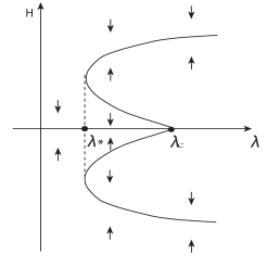
• If $B<0,$ then the phase transition of (2.13) at $\lambda_{c}$ is Type-II, where $\lambda_{c}=(|K_{1}|^{4}+\sigma)/|K_{1}|^{2}$ and $|K_{1}|^{2}=k_{1}^{2}\pi^{2}/L_{1}^{2}$. In particular, the problem bifurcates on the side $\lambda<\lambda_{c}$ to two non-degenerate saddle points, and there are two saddle-node bifurcations at some $\lambda_{\ast}<\lambda_{c}$ as shown in Figure 1(a).

  

  (a)

  

  (b)

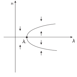
  Figure 1. (a) Type-II transition given by Theorem 4.1: The disordered state $u=0$ is globally stable when $\lambda<\lambda_{\ast}$, is metastable when $\lambda_{\ast}<\lambda<\lambda_{c}$, and becomes unstable when $\lambda>\lambda_{c}$. There are two saddle-node bifurcations at $\lambda_{\ast}$. (b) Tyep-I transition as given by Theorem 4.1.

• If $B>0$, then the transition is Type-I, and the problem bifurcates on $\lambda>\lambda_{c}$ to two attractors $u_{1}$ and $u_{2}$ as shown in Figure 1(b), which are given by (see Figure 2 for a structure of $u_{1,2}$):

  (4.4) $$u_{1,2}=\pm\sqrt{\frac{\textstyle 4\beta_{K_{1}}}{\textstyle 3\sqrt{\sigma}B}}\cos(\frac{\textstyle k_{1}\pi x_{1}}{\textstyle L_{1}})+o(|\beta_{K_{1}}|^{1/2}),$$

  where $\beta_{K_{1}}$ is given in (3.5).

Figure 2. LAM pattern: a schematic structure of $u_{1,2}$ given in (4.4).

Two remarks are now in order.

First, as we know, a Type-II transition correspond to the first-order transition in the sense of Ehrenfest. In this case, $\lambda_{\ast}$ and $\lambda_{c}$ in Figure 1(a) represent respectively the so called binodal and spinodal points. From (3.6), we know that $\lambda_{c}$ is approximately $2\sqrt{\sigma}$, then by (2.9) and (2.12), we have the following formula for the spinodal which involves only $\chi N$ and $a$ as independent parameters:

$$\chi N\approx\frac{\textstyle\sqrt{3}}{\textstyle 2(a(1-a))^{3/2}}+\frac{\textstyle a^{2}+(1-a)^{2}}{\textstyle 2a^{2}(1-a)^{2}}.$$

To our knowledge, there is no such simple formula for the binodal point. Nevertheless, some efforts have been devoted to figuring out $\lambda_{\ast}$ numerically e.g. in [5].

In addition, when the control parameter $\lambda$ is between $\lambda_{\ast}$ and $\lambda_{c}$, the disordered state $u=0$ is metastable. Perturbation may lead the system to other metastable states which may be far away from the original disordered one.

Second, Type-I transition corresponds to the second-order or higher-order transition in physics. In this case the transition states are determined by the perturbation of the first eigenvectors. In Theorem 4.1, the transition states are $u_{1,2}$, which are stable states, and represent a lamellar pattern as shown in Figure 2.

4.2. Transitions to HPC Patterns.

Now, we consider the case when the domain size satisfies the following condition:

(4.5) $$L_{1}=2\pi L,\>L_{2}=\frac{2}{\sqrt{3}}\pi L,\text{ and }L_{3}=\theta\pi L.$$

Here $L$ and $\theta$ are some positive constants, which are chosen in a way such that $K_{1}^{c}:=(\frac{n}{L},0,0)$ and $K_{2}^{c}:=(\frac{n}{2L},\frac{\sqrt{3}n}{2L},0)$ are the only wave vectors satisfying (3.6), where $n$ is a positive integer.

Theorem 4.2.

Assume that the size of the domain satisfies (4.5) and $K_{1}^{c}=(\frac{n}{L},0,0)$ and $K_{2}^{c}=(\frac{n}{2L},\frac{\sqrt{3}n}{2L},0)$ are the only two wave vectors which satisfy (3.6). Let $B$ be the parameter defined in (4.1) with $|K_{1}|=|K_{1}^{c}|=|K_{2}^{c}|$. The following assertions hold true:

• If

  $$\gamma_{2}=0,$$

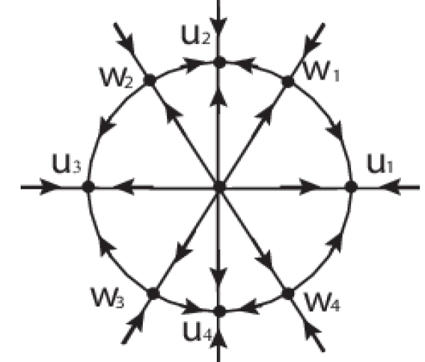
  then the phase transition of (2.13) at $\lambda_{c}$ is Type-I, where $\lambda_{c}$ is given by (3.6). The problem bifurcates on the side $\lambda>\lambda_{c}$ to an attractor $\Sigma_{\lambda}$, which is homeomorphic to the one-dimensional unit sphere $S^{1}$. $\Sigma_{\lambda}$ contains eight non-degenerate steady states, with four saddle points $w_{1}$, $w_{2}$, $w_{3}$ and $w_{4}$ and four minimal attractors $u_{1}$,$u_{2}$, $u_{3}$ and $u_{4}$ as shown in Figure 3. Moreover, we have the following approximation formulas for the steady states:

  (4.6) $$u_{1,3}= \pm\sqrt{-\frac{\beta_{1}(\lambda)}{b}}\cos(\frac{n}{d}x_{1})+o(|\beta_{1}|^{1/2}),$$

  $$u_{2,4}= \pm\sqrt{-\frac{\beta_{1}(\lambda)}{d}}\cos(\frac{n}{2d}x_{1})\cos(\frac{\sqrt{3}n}{2d}x_{2})+o(|\beta_{1}|^{1/2}),$$

  $$w_{1,2,3,4}= \pm\sqrt{-\frac{\beta_{1}(\lambda)}{b+4c}}\cos(\frac{n}{d}x_{1})$$

  $$\pm 2\sqrt{-\frac{\beta_{1}(\lambda)}{b+4c}}\cos(\frac{n}{2d}x_{1})\cos(\frac{\sqrt{3}n}{2d}x_{2})+o(|\beta_{1}|^{1/2}),$$

  where $b$ and $d$ are given in (5.16) and $\beta_{1}(\lambda)=\beta_{K^{c}_{1}}$ is as in (3.5).

• If

  $$\gamma_{2}\neq 0\text{ and }B<0,$$

  then the problem bifurcates on both sides of $\lambda_{c}$ and the transition is Type-II. Moreover, there are four steady states bifurcated out on the side $\lambda<\lambda_{c}$, including three saddle points and one unstable node. On the side $\lambda>\lambda_{c}$, the problem bifurcates to two steady states, which are saddles.

• If

  $$\gamma_{2}\neq 0\text{ and }B>0,$$

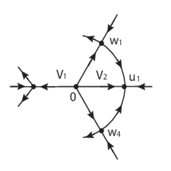
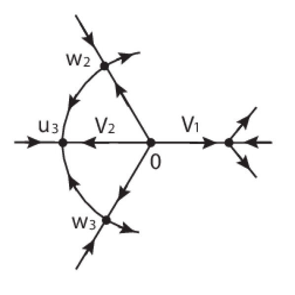
  then the transition is Type-III. Again, there are bifurcations on both sides of $\lambda_{c}=2\sqrt{\sigma}$. On the side $\lambda<\lambda_{c}$, there are two saddles bifurcating out from the origin. On the side $\lambda>\lambda_{c}$, the problem bifurcates to four steady states, including one stable node and three saddles. Moreover, there is a neighborhood $V\subset H$ of $u=0$, which can be decomposed into two disjoint sectorial regions $V_{1}$ and $V_{2}$ such that $\overline{V}=\overline{V}_{1}\cup\overline{V}_{2}$ and the phase transition is first order in $V_{1}$ and is $n$-th order in $V_{2}$ with $n\geq 2$ in the Ehrenfest sense. $V_{1}$ and $V_{2}$ satisfy the relation given in (5.18). In region $V_{2}$, there is exactly one minimal attractor as is shown in Figure 3 for $\gamma_{2}>0$ and in Figure 3 for $\gamma_{2}<0$. The minimal attractors $u_{1}$ and $u_{3}$ can again be approximated as in (4.6).

Figure 3. (a) For $\gamma_{2}=0$, the attractor $\Sigma_{\lambda}$ after the transition is homeomorphic to $S^{1}$ and $u_{1},u_{2},u_{3}$ and $u_{4}$ are minimal attractors. (b) For $\gamma_{2}>0$, the sectorial regions $V_{1}$ and $V_{2}$ are separated by the lines $\overline{0w_{1}}$ and $\overline{0w_{4}}$, and $u_{1}$ is the minimal attractor in $V_{2}$. (c) For $\gamma_{2}<0$, the sectorial regions $V_{1}$ and $V_{2}$ are separated by the lines $\overline{0w_{2}}$ and $\overline{0w_{3}}$, and $u_{3}$ is the minimal attractor in region $V_{2}$.

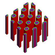
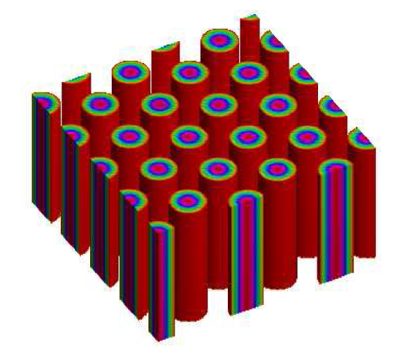
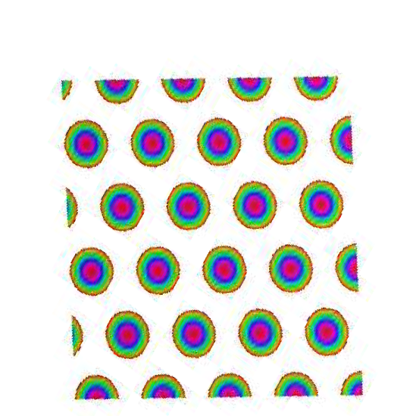
We note that, among all the steady states given in (4.6), $u_{1,3}$ are related to LAM as shown in Figure 2, $w_{1,2,3,4}$ lead to HPC given in Figure 4, and $u_{2,4}$ correspond to rectangular patterns as in Figure 6. In the case of Type-I transition, as the disordered state loses its stability, the transition happens in two stages. There is first a fast transition from the disordered state to the bifurcated attractor $\Sigma_{\lambda}$, then followed by a slow transition within the bifurcated structure. Depending on the initial perturbations, the patterns finally emerging from the transition may be either lamellae or rectangles.

In Type-III transition case, transition may happen on both sides of the critical point $\lambda_{c}$. On the side $\lambda<\lambda_{c}$, the disordered state is metastable, and perturbations may lead the system to some other metastable states far away from the disordered state as discussion in last section. On the side $\lambda>\lambda_{c}$, the disordered state is unstable, and the transition may be either first order or second order depending on the initial perturbations. When the perturbation leads to second order transition, there is first a fast transition to the local attractor composed with two steady states with the HPC structure, one steady state with LAM structure, and two heteroclinic orbits connecting them as shown in Figures 3 and 3. The pattern eventually goes to LAM.

Figure 4. (a) HPC structures determined by $w_{1,2,3,4}$ in (4.6). (b) Top view of the structures given in part (a).

4.3. Transitions to Squares and Spheres

In this section, we return to the situation when the first eigenvalue is simple, and we study the case when the corresponding $K_{1}$ satisfying (3.6) is of the form $K_{1}=(k_{1}\pi/L_{1},\ k_{2}\pi/L_{2},\ 0)$, $k_{i}\neq 0$, $1\leq i\leq 2$, or $K_{1}=(k_{1}\pi/L_{1},\ k_{2}\pi/L_{2},\ k_{3}\pi/L_{3})$, $k_{i}\neq 0$, $1\leq i\leq 3$. For simplicity, we will give results for the case $k_{1}/L_{1}=k_{2}/L_{2}=k_{3}/L_{3}$, but the general situation can be dealt with in the same way. With this assumption, the first critical eigenvectors will have square pattern when $K_{1}=(k_{1}\pi/L_{1},\ k_{2}\pi/L_{2},\ 0)$, and a cubic pattern when $K_{1}=(k_{1}\pi/L_{1},\ k_{2}\pi/L_{2},\ k_{3}\pi/L_{3})$. We define the following parameters:

(4.7) $$B_{2}=\gamma_{3}-\frac{16}{9}\left(\frac{|K_{1}|^{2}}{2|K_{1}|^{4}-\sigma}+\frac{1}{2}\frac{\textstyle|K_{1}|^{2}}{\textstyle 14|K_{1}|^{4}-2\lambda|K_{1}|^{2}-\sigma}\right)\gamma_{2}^{2},$$

$$B_{3}=\gamma_{3}-\frac{32|K_{1}|^{2}}{3}\biggl{(}\frac{1}{-2|K_{1}|^{4}+6\lambda|K_{1}|^{2}-9\sigma}+\frac{1}{46|K_{1}|^{4}-6\lambda|K_{1}|^{2}-9\sigma}$$

$$\hskip 108.405pt+\frac{1}{252|K_{1}|^{4}-108\lambda|K_{1}|^{2}-18\sigma}\biggr{)}\gamma_{2}^{2}.$$

Using (4.2), we have

(4.8) $$B_{2}\simeq\gamma_{3}-\frac{\textstyle 152}{\textstyle 81}\frac{\gamma_{2}^{2}}{\sqrt{\sigma}},$$

$$B_{3}\simeq\gamma_{3}-(11+\frac{\textstyle 463}{\textstyle 675})\frac{\gamma_{2}^{2}}{\sqrt{\sigma}}.$$

Theorem 4.3.

Assume that $K_{1}=(k_{1}\pi/L_{1},\ k_{2}\pi/L_{2},\ 0)$, $k_{1}/L_{1}=k_{2}/L_{2}\neq 0$, is the only wave vector which satisfies (3.6). Then the following assertions hold true:

• If

  $$B_{2}<0,$$

  then the phase transition of (2.13) at $\lambda_{c}$ is Type-II, where the critical value $\lambda_{c}$ is given by (3.6). In particular, the problem bifurcates from $(u,\,\lambda)=(0,\,\lambda_{c})$ on the side $\lambda<\lambda_{c}$ to two non-degenerate saddle points, and there are two saddle-node bifurcations at some $\lambda_{\ast}<\lambda_{c}$.

• If

  $$B_{2}>0,$$

  the transition is Type-I, and the problem bifurcates on $\lambda>\lambda_{c}$ to two attractors $u_{1}$ and $u_{2}$, which can be expressed as (see Figure 6 for the structure of $u_{1,2}$)

  (4.9) $$u_{1,2}=\pm\sqrt{\frac{\textstyle 16\beta_{K_{1}}}{\textstyle 9\sqrt{\sigma}B_{2}}}\cos(\frac{\textstyle k_{1}\pi x_{1}}{\textstyle L_{1}})\cos(\frac{\textstyle k_{2}\pi x_{2}}{\textstyle L_{2}})+o(|\beta_{K_{1}}|^{1/2}),$$

  where $\beta_{K_{1}}$ is as in (3.5).

0.8

Figure 5. Rectangular patterns: a schematic structure of $u_{1,2}$ given in (4.9).

0.8

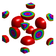
Figure 6. Sphere patterns in face-centered-cubic lattices: a schematic structure of $u_{1,2}$ given in (4.10).

Theorem 4.4.

Assume that the only wave vector which satisfies (3.6) is $K_{1}=(k_{1}\pi/L_{1},\ k_{2}\pi/L_{2},\ k_{3}\pi/L_{3})$, $k_{1}/L_{1}=k_{2}/L_{2}=k_{3}/L_{3}\neq 0$. Then the following assertions hold true:

• If

  $$B_{3}<0,$$

  then the phase transition of (2.13) at $\lambda_{c}$ is Type-II, where the critical value $\lambda_{c}$ is given by (3.6). In particular, the problem bifurcates on the side $\lambda<\lambda_{c}$ to two non-degenerate saddle points, and there are two saddle-node bifurcations.

• If

  $$B_{3}>0,$$

  the transition is Type-I, and the problem bifurcates on $\lambda>\lambda_{c}$ to two attractors $u_{1}$ and $u_{2}$, which can be expressed as (see Figure 6 for the structure of $u_{1,2}$)

  (4.10) $$u_{1,2}=\pm\sqrt{\frac{\textstyle 64\beta_{K_{1}}}{\textstyle 27\sqrt{\sigma}B_{3}}}\cos(\frac{\textstyle k_{1}\pi x_{1}}{\textstyle L_{1}})\cos(\frac{\textstyle k_{2}\pi x_{2}}{\textstyle L_{2}})\cos(\frac{\textstyle k_{3}\pi x_{3}}{\textstyle L_{3}})+o(|\beta_{K_{1}}|^{1/2}),$$

  where $\beta_{K_{1}}$ is as in (3.5).

5. Proofs of Main Theorems

Proof of Theorem 4.1.

The proof relies on the following center manifold reduction, which reduce equation (2.13) to a one-dimensional ODE.

Let $u=v+\Phi(y,\lambda)$, where $v=ye_{K_{1}}$, and $\Phi$ is the center manifold function which we will calculate later. Thanks to the classical center manifold theorem [12, 28, 18], we have $\langle v,\,\Phi\rangle_{H}=0$ and $\Phi(y,\lambda)=o(|y|)$. Now multiplying both sides of (2.13) by $e_{K_{1}}$ and integrating over $\Omega$, we obtain the reduced equation to the center manifold:

(5.1) $$\frac{\textstyle\mathrm{d}y}{\textstyle\mathrm{d}t}=\beta_{K_{1}}(\lambda)y-\frac{\textstyle 2k_{1}^{2}\pi^{2}}{\textstyle L_{1}^{2}|\Omega|}g(y)+o(|y|^{3}),$$

where $|\Omega|$ is the volume of $\Omega$, and

(5.2) $$g(y) = G_{2}(y)+G_{3}(y)+G_{23}(y),$$

(5.3) $$G_{2}(y) = \gamma_{2}\int_{\Omega}v^{2}e_{K_{1}}\,\mathrm{d}x,$$

(5.4) $$G_{3}(y) = \gamma_{3}\int_{\Omega}v^{3}e_{K_{1}}\,\mathrm{d}x,$$

(5.5) $$G_{23}(y) = 2\gamma_{2}\int_{\Omega}v\Phi(y,\,\lambda)e_{K_{1}}\,\mathrm{d}x.$$

By direct computation, we know

(5.6) $$G_{2}=\int_{\Omega}(y\cos(k_{1}\pi x_{1})/L_{1})^{2}\cos(k_{1}\pi x_{1}/L_{1})\,\mathrm{d}x=0,$$

(5.7) $$G_{3}=\int_{\Omega}(y\cos(k_{1}\pi x_{1}/L_{1}))^{3}\cos(k_{1}\pi x_{1}/L_{1})\,\mathrm{d}x=\frac{\textstyle 3\gamma_{3}}{\textstyle 8}|\Omega|y^{3}.$$

To evaluate $G_{23}$, we need to compute the center manifold function $\Phi(y,\,\lambda)$. We will use the following second order approximation formula of $\Phi(y,\,\lambda)$ (see e.g. [17] for details):

(5.8) $$-\mathcal{L}_{\lambda}\Phi(y,\lambda)=P_{2}G_{2}(y,\lambda)+O(|\beta(\lambda)||y|^{2})+o(|y|^{2}).$$

Here $P_{2}:H\rightarrow H_{2}^{\lambda}$ is the canonical projection with $H_{2}^{\lambda}$ being the subspace of $H$ spanned by all stable eigenfunctions of $L_{\lambda}$, $\mathcal{L}_{\lambda}$ is the restriction of $L_{\lambda}$ to $H_{2}^{\lambda}$, and $\beta(\lambda)$ is the first eigenvalue of $L_{\lambda}$.

The above formula (5.8) implies that

$$\Phi(y,\lambda) =\sum_{K\in\mathcal{P},K\neq K_{1}}\Phi_{K}(y,\lambda)e_{K}+o(|y|^{2}),\quad\text{where}$$

$$\Phi_{K}(y,\lambda) =\frac{\textstyle\gamma_{2}}{\textstyle(2\beta_{K_{1}}(\lambda)-\beta_{K})\langle e_{K},\,e_{K}\rangle_{H}}\int_{\Omega}\Delta v^{2}e_{K}\,\mathrm{d}x$$

$$=-\frac{\textstyle\gamma_{2}\rho_{K}}{\textstyle(2\beta_{K_{1}}(\lambda)-\beta_{K})\langle e_{K},\,e_{K}\rangle_{H}}\int_{\Omega}v^{2}e_{K}\,\mathrm{d}x.$$

Note that

$$\int_{\Omega}e_{K_{1}}^{2}e_{K}\,\mathrm{d}x=\int_{\Omega}\frac{\textstyle 1+\cos(2k_{1}\pi x_{1}/L_{1})}{\textstyle 2}e_{K}\,\mathrm{d}x\\ =0\text{\> unless \>}K=(2k_{1}\pi/L_{1},\,0,\,0).$$

For $K=(2k_{1}\pi/L_{1},\,0,\,0)$, we have:

(5.9) $$\Phi_{K}(y,\lambda)=-2\xi\gamma_{2}y^{2},$$

where $\xi=\frac{\textstyle k_{1}^{2}\pi^{2}/L_{1}^{2}}{\textstyle 14k_{1}^{4}\pi^{4}/L_{1}^{4}-2\lambda k_{1}^{2}\pi^{2}/L_{1}^{2}-\sigma}$.

Thus we obtain the center manifold function as follows:

(5.10) $$\Phi(y,\lambda)=-2\xi\gamma_{2}y^{2}\cos(\frac{\textstyle 2k_{1}\pi x_{1}}{\textstyle L_{1}})+o(|y|^{2}).$$

Plugging (5.10) into (5.5), we find

(5.11) $$G_{23}=-\xi|\Omega|\gamma^{2}_{2}y^{3}+o(|y|^{3}).$$

Finally, plugging (5.2), (5.6), (5.7) and (5.11) into (5.1), we can derive the following reduced equation of (2.13):

(5.12) $$\frac{\mathrm{d}y}{\mathrm{d}t}=\beta_{K_{1}}(\lambda)y-\frac{\textstyle 2k_{1}^{2}\pi^{2}}{\textstyle L_{1}^{2}}\Bigl{(}\frac{\textstyle 3}{\textstyle 8}\gamma_{3}-\frac{k_{1}^{2}\pi^{2}/L_{1}^{2}}{\frac{14k_{1}^{4}\pi^{4}}{L_{1}^{4}}-\frac{2\lambda k_{1}^{2}\pi^{2}}{L_{1}^{2}}-\sigma}\gamma_{2}^{2}\Bigr{)}y^{3}+o(|y|^{3}).$$

It is known from [17, 18] that the transition type of (2.13) at the critical point $\lambda_{c}$ is completely determined by (5.12). Thus all the assertions of the theorem follow from (5.12) except the claim for the saddle-node bifurcation in Assertion (1), which we prove as follows.

When $\gamma_{3}<\frac{\textstyle 8|K_{1}|^{2}}{\textstyle 36|K_{1}|^{4}-9\sigma}\gamma_{2}^{2}$, we know from (5.12) that there are two branches of saddle points bifurcating from $(u,\,\lambda)=(0,\,\lambda_{c})$. The result will follow if we can show that there exists $\widetilde{\lambda}<\lambda_{c}$ such that the following two conditions hold:

1. $u=0$ is globally stable for any $\lambda<\widetilde{\lambda}$.

2. The two branches of saddle points are uniformly bounded when $\widetilde{\lambda}<\lambda<\lambda_{c}$.

To verify (i), we do an energy estimate. For any $\lambda<\widetilde{\lambda}=-\gamma_{2}^{2}/2\gamma_{3}$, and $u\neq 0$ in $H$, multiplying the right hand side of (2.13) by $u$, and integrating over $\Omega$, we get:

$$\int_{\Omega}-|\Delta u|^{2}+\lambda|\nabla u|^{2}-2\gamma_{2}u|\nabla u|^{2}-3\gamma_{3}u^{2}|\nabla u|^{2}-\sigma u^{2}\,\mathrm{d}x$$

$$\leq\int_{\Omega}|\nabla u|^{2}(\lambda+2|\gamma_{2}u|-3\gamma_{3}u^{2})-\sigma u^{2}\,\mathrm{d}x$$

$$\leq\int_{\Omega}|\nabla u|^{2}(\lambda-\gamma_{3}u^{2}-2\gamma_{3}(|u|-\frac{\textstyle|\gamma_{2}|}{\textstyle 2\gamma_{3}})^{2}+\frac{\textstyle\gamma_{2}^{2}}{\textstyle 2\gamma_{3}})-\sigma u^{2}\,\mathrm{d}x$$

$$\leq\int_{\Omega}|\nabla u|^{2}(\lambda+\frac{\textstyle\gamma_{2}^{2}}{\textstyle 2\gamma_{3}})-\sigma u^{2}\,\mathrm{d}x$$

$$<0.$$

Therefore, when $\lambda<\widetilde{\lambda}$, (2.13) has no non-trivial singular points in $H$. It is known that for any $\lambda\in\mathbb{R}^{1}$, (2.13) possesses a global attractor. Thus condition (i) follows. Condition (ii) is a direct consequence of the existence of global attractors for any $\lambda\in\mathbb{R}^{1}$. The claim for saddle-node bifurcations is thus proven, and the proof is complete. ∎

Proof of Theorem 4.2.

The eigenvectors of $L_{\lambda}$ corresponding to $K_{1}^{c}$ and $K_{2}^{c}$ are

(5.13) $$e_{1}=\cos(\frac{n}{d}x_{1}),$$

$$e_{2}=\cos(\frac{n}{2d}x_{1})\cos(\frac{\sqrt{3}n}{2d}x_{2}).$$

Let $u=v+\Phi(v,\lambda)$, where $v=y_{1}e_{1}+y_{2}e_{2}$ and $\Phi$ is the center manifold function. Again, $\Phi$ can be approximated to the second order via the formula given in (5.8). In this case, we have

(5.14) $$\Phi(y,\lambda)= -\frac{2\gamma_{2}|K^{c}_{1}|^{2}y_{1}^{2}}{14|K^{c}_{1}|^{4}-2\lambda|K^{c}_{1}|^{2}-\sigma}\cos(\frac{2n}{d}x_{1})$$

$$-\frac{3\gamma_{2}|K^{c}_{1}|^{2}y_{1}y_{2}}{7|K^{c}_{1}|^{4}-\lambda|K^{c}_{1}|^{2}-\sigma}\cos(\frac{3n}{2d}x_{1})\cos(\frac{\sqrt{3}n}{2d}x_{2})$$

$$-\frac{\gamma_{2}|K^{c}_{1}|^{2}y_{2}^{2}}{14|K^{c}_{1}|^{4}-2\lambda|K^{c}_{1}|^{2}-\sigma}\cos(\frac{n}{d}x_{1})\cos(\frac{\sqrt{3}n}{d}x_{2})$$

$$-\frac{3\gamma_{2}|K^{c}_{1}|^{2}y_{2}^{2}}{28|K^{c}_{1}|^{4}-4\lambda|K^{c}_{1}|^{2}-4\sigma}\cos(\frac{\sqrt{3}n}{d}x_{2})+o(|y|^{2}),$$

where $|K_{1}^{c}|=|K_{2}^{c}|=n/L$.

The reduced equation to the center manifold is now given by

(5.15) $$\frac{\mathrm{d}y_{1}}{\mathrm{d}t} =\beta_{1}(\lambda)y_{1}-\frac{|K^{c}_{1}|^{2}\gamma_{2}}{4}y_{2}^{2}+by_{1}^{3}+cy_{1}y_{2}^{2}+o(|y|^{3}),$$

$$\frac{\mathrm{d}y_{2}}{\mathrm{d}t} =\beta_{1}(\lambda)y_{2}-|K^{c}_{1}|^{2}\gamma_{2}y_{1}y_{2}+dy_{2}^{3}+ey_{1}^{2}y_{2}+o(|y|^{3}),$$

where $\beta_{1}(\lambda)=\beta_{K_{1}^{c}}(\lambda)=\beta_{K_{2}^{c}}(\lambda)$ and

$$b =\frac{2|K^{c}_{1}|^{4}\gamma_{2}^{2}}{14|K^{c}_{1}|^{4}-2\lambda|K^{c}_{1}|^{2}-\sigma}-\frac{3|K^{c}_{1}|^{2}}{4}\gamma_{3},$$

$$c =\frac{3|K^{c}_{1}|^{4}\gamma_{2}^{2}}{14|K^{c}_{1}|^{4}-2\lambda|K^{c}_{1}|^{2}-2\sigma}-\frac{3|K^{c}_{1}|^{2}}{4}\gamma_{3},$$

$$d =\frac{|K^{c}_{1}|^{4}\gamma_{2}^{2}}{28|K^{c}_{1}|^{4}-4\lambda|K^{c}_{1}|^{2}-2\sigma}+\frac{3|K^{c}_{1}|^{4}\gamma_{2}^{2}}{28|K^{c}_{1}|^{4}-4\lambda|K^{c}_{1}|^{2}-4\sigma}-\frac{9|K^{c}_{1}|^{2}}{16}\gamma_{3},$$

$$e =\frac{3|K^{c}_{1}|^{4}\gamma_{2}^{2}}{7|K^{c}_{1}|^{4}-\lambda|K^{c}_{1}|^{2}-\sigma}-\frac{3|K^{c}_{1}|^{2}}{2}\gamma_{3}.$$

As before, we have $|K^{c}_{1}|^{2}\simeq\sqrt{\sigma}$. Then when $\lambda$ is close to $\lambda_{c}$, the above coefficients can be written as

(5.16) $$b \simeq\frac{2}{9}\gamma_{2}^{2}-\frac{3\sqrt{\sigma}}{4}\gamma_{3}+o(|\lambda-\lambda_{c}|),$$

$$c \simeq\frac{3}{8}\gamma_{2}^{2}-\frac{3\sqrt{\sigma}}{4}\gamma_{3}+o(|\lambda-\lambda_{c}|),$$

$$d \simeq\frac{35}{144}\gamma_{2}^{2}-\frac{9\sqrt{\sigma}}{16}\gamma_{3}+o(|\lambda-\lambda_{c}|),$$

$$e \simeq\frac{3}{4}\gamma_{2}^{2}-\frac{3\sqrt{\sigma}}{2}\gamma_{3}+o(|\lambda-\lambda_{c}|).$$

It is known that the transition of (5.15) near $\lambda=\lambda_{c}$ can be understood by studying the behavior of the equation when $\lambda$ is at the critical point $\lambda_{c}=(|K^{c}_{1}|^{4}+\sigma)/|K^{c}_{1}|^{2}$. At $\lambda=\lambda_{c}$, $\beta_{1}(\lambda)=0$, and (5.15) reads (up to 3rd order terms):

(5.17) $$\frac{\mathrm{d}y_{1}}{\mathrm{d}t} =-\frac{|K^{c}_{1}|^{2}\gamma_{2}}{4}y_{2}^{2}+by_{1}^{3}+cy_{1}y_{2}^{2},$$

$$\frac{\mathrm{d}y_{2}}{\mathrm{d}t} =-|K^{c}_{1}|^{2}\gamma_{2}y_{1}y_{2}+dy_{2}^{3}+ey_{1}^{2}y_{2}.$$

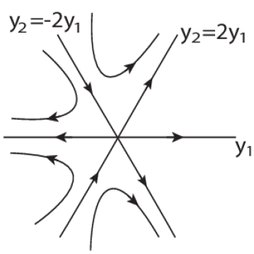
Note that by (5.16) we have $b+4c=4d+e$, from which we see that on the straight lines $y_{2}=\pm 2y_{1}$, the equation (5.17) satisfies that

$$\frac{\mathrm{d}y_{2}}{\mathrm{d}y_{1}}=\pm 2,\text{ for all }y_{1}\text{ such that }-|K^{c}_{1}|^{2}\gamma_{2}y_{1}^{2}+(b+4c)y_{1}^{3}\neq 0.$$

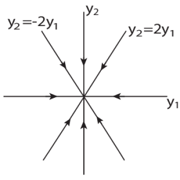
Hence, the straight lines $y_{2}=\pm 2y_{1}$ are orbits of (5.17). Obviously, $y_{2}=0$ also consists of orbits of (5.17). If $\gamma_{2}\neq 0$, all straight line orbits of (5.17) lie on one of these three lines. If $\gamma_{2}=0$, $y_{1}=0$ also consists of orbits of (5.17), and in this case all straight line orbits lie on one of four straight lines $y_{2}=\pm 2y_{1}$, $y_{2}=0$ or $y_{1}=0$.

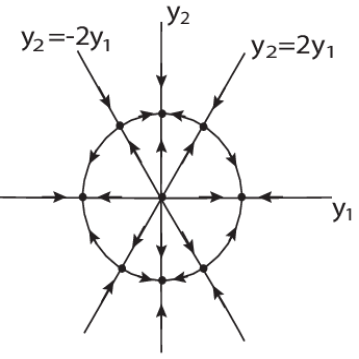
Figure 7. The topological structure of flows of (5.15), (a) for $\gamma_{2}=0$ and $\beta_{1}(\lambda)=0$, and (b) for $\gamma_{2}=0$ and $\beta_{1}(\lambda)>0$.

For the case $\gamma_{2}=0$, the numbers $b$, $c$, $d$, and $e$ are all less than zero by (2.11) and (5.16). It is easy to see that all the straight line orbits of (5.17) tend to the origin as shown in Figure 7, which implies that the origin $(y_{1},y_{2})=(0,0)$ is locally asymptotically stable. Therefore, the transition of (5.15) is Type-I [18]. Omitting $o(|y|^{3})$ terms in (5.15), the bifurcated structure are shown in Figure 7. The origin becomes unstable, and there are eight other steady states emerging from the transition, among which four of them are stable and the rest are saddle points. The stability of the steady states can be analyzed by linearizing (5.15) about the corresponding steady state, and the results are shown in Figure 7. By the center manifold reduction, the bifurcated structure for the original equation (2.13) is a perturbation of the structure shown in Figure 7, and Assertion (1) is thus proved.

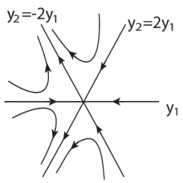
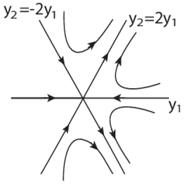
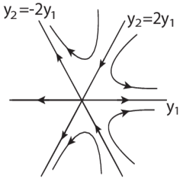
Figure 8. The topological structure of flows of (5.17), (a) for $\gamma_{2}>0$ and $b>0$, (b) for $\gamma_{2}<0$ and $b>0$, (c) for $\gamma_{2}>0$ and $b<0$, and (b) for $\gamma_{2}<0$ and $b<0$.

When $\gamma_{2}\neq 0$, the straight line orbits of (5.17) consist of $y_{2}=\pm 2y_{1}$ and $y_{2}=0$ as shown before. The phase diagram of (5.17) near the origin can now be easily determined and are shown in Figures 8 – 8.

For $\gamma_{2}\neq 0$ and $b>0$, a neighborhood of the origin is divided into six regions by the straight line orbits, and four of them are hyperbolic and the rest two regions are parabolic as shown in Figures 8 and 8. Since orbits starting from any of these regions are eventually repelled away from the origin, the transition is Type-II [17]. The number and type of equilibrium points bifurcated out for each case can be analyzed in the same fashion as in the proof for Assertion (1), thus Assertion (2) is proved.

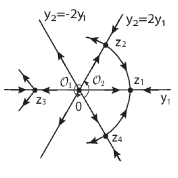
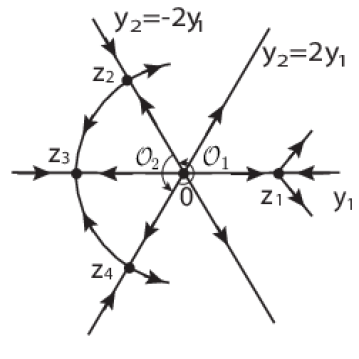
For $\gamma_{2}\neq 0$ and $b<0$, a neighborhood of the origin is also divided into six regions by the straight line orbits, and four of them are hyperbolic and the rest two regions are parabolic as shown in Figures 8 and 8. Here, orbits in the parabolic regions tend to the origin, and the transition is Type-III [17]. The flow structure of the reduced equation (5.15) when $\lambda>\lambda_{c}$ can also be obtained easily and the result after dropping $o(|y|^{3})$ terms is shown in Figure 9.

Figure 9. The topological structure of flows of (5.15) for $\lambda>\lambda_{c}$, $b<0$ and (a) for $\gamma_{2}>0$, (b) for $\gamma_{2}<0$. The two sectorial regions $\mathcal{O}_{1}$ and $\mathcal{O}_{2}$ are seperated by the rays $\overline{0z_{2}}$ and $\overline{0z_{4}}$.

From here, we see that there is a neighborhood $\mathcal{N}$ of the origin of the $y_{1}y_{2}$ plane, which can be decomposed into two disjoint regions $\mathcal{N}_{1}$ and $\mathcal{N}_{2}$ such that $\overline{\mathcal{N}}=\overline{\mathcal{N}}_{1}\cup\overline{\mathcal{N}}_{2}$ and in region $\mathcal{N}_{2}$, there is exactly one stable node bifurcating out on the side $\lambda>\lambda_{c}$. Actually, $\mathcal{N}_{1}$ and $\mathcal{N}_{2}$ are slight perturbations of $\mathcal{O}_{1}$ and $\mathcal{O}_{2}$ respectively as shown in Figure 9. Corresponding to $\mathcal{N}$, there is a neigborhood $V$ of the origin in space $H$, which can be decomposed into two disjoint regions $V_{1}$ and $V_{2}$ such that $\overline{V}=\overline{V_{1}}\cup\overline{V_{2}}$. Here $V_{1}$ and $V_{2}$ are chosen such that

(5.18) $$(1-P_{2})V_{i}=\mathcal{N}_{i},\>1\leq i\leq 2,$$

where $P_{2}$ is the canonical projection as in (5.8). Thus, assertion (3) is proved and the proof is complete. ∎

The proofs of Theorem 4.3 and Theorem 4.4 are similar to that of Theorem 4.1, and the details are omitted here. But for the convenience of the readers, we present the center manifold functions and the reduced equations to the center manifold.

Proof of Theorem 4.3.

By similar calculation, we have the following center manifold function:

$$\Phi(y,\lambda)=-\xi_{1}\gamma_{2}y^{2}\cos(\frac{\textstyle 2k_{1}\pi x_{1}}{\textstyle L_{1}})-\xi_{2}\gamma_{2}y^{2}\cos(\frac{\textstyle 2k_{2}\pi x_{2}}{\textstyle L_{2}})$$

$$-\xi_{3}\gamma_{2}y^{2}\cos(\frac{\textstyle 2k_{1}\pi x_{1}}{\textstyle L_{1}})\cos(\frac{\textstyle 2k_{2}\pi x_{2}}{\textstyle L_{2}})+o(|y|^{2}).$$

Here $\xi_{1}$, $\xi_{2}$ and $\xi_{3}$ are as follows:

$$\xi_{1}(\lambda)=\frac{\textstyle|K_{11}|^{2}}{\textstyle 14|K_{11}|^{4}-4|K_{11}|^{2}|K_{12}|^{2}-2|K_{12}|^{4}+2\lambda(|K_{12}|^{2}-|K_{11}|^{2})-\sigma},$$

$$\xi_{2}(\lambda)=\frac{\textstyle|K_{12}|^{2}}{\textstyle 14|K_{12}|^{4}-4|K_{11}|^{2}|K_{12}|^{2}-2|K_{11}|^{4}+2\lambda(|K_{11}|^{2}-|K_{12}|^{2})-\sigma},$$

$$\xi_{3}(\lambda)=\frac{\textstyle|K_{1}|^{2}}{\textstyle 14|K_{1}|^{4}-2\lambda|K_{1}|^{2}-\sigma},$$

where $|K_{11}|^{2}=\frac{\textstyle k_{1}^{2}\pi^{2}}{\textstyle L_{1}^{2}},\quad|K_{12}|^{2}=\frac{\textstyle k_{2}^{2}\pi^{2}}{\textstyle L_{2}^{2}},\quad|K_{1}|^{2}=\frac{\textstyle k_{1}^{2}\pi^{2}}{\textstyle L_{1}^{2}}+\frac{\textstyle k_{2}^{2}\pi^{2}}{\textstyle L_{2}^{2}}.$

The reduced equations of (2.13) to the center manifold in this case is:

$$\frac{\mathrm{d}y}{\mathrm{d}t}=\beta_{K_{1}}(\lambda)y-|K_{1}|^{2}\Big{(}\frac{\textstyle 9}{\textstyle 16}\gamma_{3}-\big{(}\xi_{1}(\lambda)+\xi_{2}(\lambda)+\frac{\textstyle 1}{\textstyle 2}\xi_{3}(\lambda)\big{)}\gamma_{2}^{2}\Big{)}y^{3}+o(|y|^{3}).$$

∎

Proof of Theorem 4.4.

The center manifold function for this case is:

$$\Phi(y,\lambda) =-\eta_{1}\gamma_{2}y^{2}\cos(\frac{\textstyle 2k_{1}\pi x_{1}}{\textstyle L_{1}})-\eta_{2}\gamma_{2}y^{2}\cos(\frac{\textstyle 2k_{2}\pi x_{2}}{\textstyle L_{2}})$$

$$-\eta_{3}\gamma_{2}y^{2}\cos(\frac{\textstyle 2k_{3}\pi x_{3}}{\textstyle L_{3}})-\eta_{4}\gamma_{2}y^{2}\cos(\frac{\textstyle 2k_{1}\pi x_{1}}{\textstyle L_{1}})\cos(\frac{\textstyle 2k_{2}\pi x_{2}}{\textstyle L_{2}})$$

$$-\eta_{5}\gamma_{2}y^{2}\cos(\frac{\textstyle 2k_{1}\pi x_{1}}{\textstyle L_{1}})\cos(\frac{\textstyle 2k_{3}\pi x_{3}}{\textstyle L_{3}})-\eta_{6}\gamma_{2}y^{2}\cos(\frac{\textstyle 2k_{2}\pi x_{2}}{\textstyle L_{2}})\cos(\frac{\textstyle 2k_{3}\pi x_{3}}{\textstyle L_{3}})$$

$$-\eta_{7}\gamma_{2}y^{2}\cos(\frac{\textstyle 2k_{1}\pi x_{1}}{\textstyle L_{1}})\cos(\frac{\textstyle 2k_{2}\pi x_{2}}{\textstyle L_{2}})\cos(\frac{\textstyle 2k_{3}\pi x_{3}}{\textstyle L_{3}})+o(|y|^{2}),$$

and the reduced equations of (2.13) to the center manifold is given by:

$$\frac{\mathrm{d}y}{\mathrm{d}t}=\beta_{K_{1}}(\lambda)y-|K_{1}|^{2}(\frac{\textstyle 27}{\textstyle 64}\gamma_{3}-\eta\gamma_{2}^{2})y^{3}+o(|y|^{3}),$$

Here $\eta$ and $\eta_{i}$ $(1\leq i\leq 7)$ are given by

$$\eta_{1}(\lambda)=\frac{\textstyle k_{1}^{2}\pi^{2}/L_{1}^{2}}{\textstyle 2\bigl{[}-2|K_{1}|^{4}+\frac{\textstyle 16k_{1}^{4}\pi^{4}}{\textstyle L_{1}^{4}}+\lambda(2|K_{1}|^{2}-\frac{\textstyle 4k_{1}^{2}\pi^{2}}{\textstyle L_{1}^{2}})-\sigma\bigr{]}},$$

$$\eta_{2}(\lambda)=\frac{\textstyle k_{2}^{2}\pi^{2}/L_{2}^{2}}{\textstyle 2\bigl{[}-2|K_{1}|^{4}+\frac{\textstyle 16k_{2}^{4}\pi^{4}}{\textstyle L_{2}^{4}}+\lambda(2|K_{1}|^{2}-\frac{\textstyle 4k_{2}^{2}\pi^{2}}{\textstyle L_{2}^{2}})-\sigma\bigr{]}},$$

$$\eta_{3}(\lambda)=\frac{\textstyle k_{3}^{2}\pi^{2}/L_{3}^{2}}{\textstyle 2\bigl{[}-2|K_{1}|^{4}+\frac{\textstyle 16k_{3}^{4}\pi^{4}}{\textstyle L_{3}^{4}}+\lambda(2|K_{1}|^{2}-\frac{\textstyle 4k_{3}^{2}\pi^{2}}{\textstyle L_{3}^{2}})-\sigma\bigr{]}},$$

$$\eta_{4}(\lambda)=\frac{\textstyle|K_{12}|^{2}}{\textstyle 2\bigl{[}-2|K_{1}|^{4}+16|K_{12}|^{4}+2\lambda(|K_{1}|^{2}-2|K_{12}|^{2})-\sigma\bigr{]}},$$

$$\eta_{5}(\lambda)=\frac{\textstyle|K_{13}|^{2}}{\textstyle 2\bigl{[}-2|K_{1}|^{4}+16|K_{13}|^{4}+2\lambda(|K_{1}|^{2}-2|K_{13}|^{2})-\sigma\bigr{]}},$$

$$\eta_{6}(\lambda)=\frac{\textstyle|K_{23}|^{2}}{\textstyle 2\bigl{[}-2|K_{1}|^{4}+16|K_{23}|^{4}+2\lambda(|K_{1}|^{2}-2|K_{23}|^{2})-\sigma\bigr{]}},$$

$$\eta_{7}(\lambda)=\frac{\textstyle|K_{1}|^{2}}{\textstyle 14|K_{1}|^{4}-2\lambda|K_{1}|^{2}-\sigma},$$

$$\eta(\lambda)=\eta_{1}+\eta_{2}+\eta_{3}+\frac{\textstyle 1}{\textstyle 2}(\eta_{4}+\eta_{5}+\eta_{6})+\frac{\textstyle 1}{\textstyle 4}\eta_{7},$$

where

$$|K_{12}|^{2}=\frac{\textstyle k_{1}^{2}\pi^{2}}{\textstyle L_{1}^{2}}+\frac{\textstyle k_{2}^{2}\pi^{2}}{\textstyle L_{2}^{2}}, |K_{13}|^{2}=\frac{\textstyle k_{1}^{2}\pi^{2}}{\textstyle L_{1}^{2}}+\frac{\textstyle k_{3}^{2}\pi^{2}}{\textstyle L_{3}^{2}},$$

$$|K_{23}|^{2}=\frac{\textstyle k_{2}^{2}\pi^{2}}{\textstyle L_{2}^{2}}+\frac{\textstyle k_{3}^{2}\pi^{2}}{\textstyle L_{3}^{2}}, |K_{1}|^{2}=\frac{\textstyle k_{1}^{2}\pi^{2}}{\textstyle L_{1}^{2}}+\frac{\textstyle k_{2}^{2}\pi^{2}}{\textstyle L_{2}^{2}}+\frac{\textstyle k_{3}^{2}\pi^{2}}{\textstyle L_{3}^{2}}.$$

∎

References

• [1] F. S. Bates and G. H. Fredrickson. Block copolymer thermodynamics: theory and experiment. Annu. Rev. Phys. Chem., 41:525–557, 1990.
• [2] F. S. Bates and G. H. Fredrickson. Block copolymers – designer soft materials. Physics Today, 52:32–38, 1999.
• [3] F. S. Bates and M. W. Matsen. Unifying weak- and strong-segragation block copolymer theories. Macromolecules, 29(4):1091–1098, 1996.
• [4] J. W. Cahn. Spinodal decomposition. Tran. Meta. Soc. AIME, 242:166–180, 1968.
• [5] R. Choksi, M. A. Peletier, and J. F. Williams. On the phase diagram for microphase separation of diblock copolymers: An approach via a nonlocal  cahn-hilliard functional. SIAM J. Appl. Math., 69(6):1712–1738, 2009.
• [6] R. Choksi and X. Ren. On the derivation of a density functional theory for microphase separation of diblock copolymers. J. Stat. Phys., 113:151–176, 2003.
• [7] P. de Gennes. Scaling concepts in polymer physics. Cornell university press, 1979.
• [8] P. de Gennes. Dynamics of fluctuations and spinodal decomposition in polymer blends. J. Chem. Phys., 72(1):4756–4763, 1980.
• [9] R. C. Desai and R. Kapral. Dynamics of Self-Organized and Self-Assembled Structures. Cambridge University Press, 2009.
• [10] P. J. Flory and W. R. Krigbaum. Thermodynamics of high polymer solutions. Annu. Rev. Phys. Chem., 2:383–402, 1951.
• [11] G. H. Fredrickson, V. Ganesan, and F. Drolet. Field-theoretic computer simulation methods for polymers and complex fluids. Macromolecules, 35:16–39, 2002.
• [12] D. Henry. Geometric theory of semilinear parabolic equations, volume 840 of Lecture Notes in Mathematics. Springer-Verlag, Berlin, 1981.
• [13] M. L. Huggins. Solutions of long chain compounds. J. Chem. Phys., 9:440, 1941.
• [14] K. Jiang, C. Wang, Y. Huang, and P. Zhang. Metastable patterns in diblock copolymers. submitted to J. chem. Phys.
• [15] T. Kawakatsu. Statistical physics of polymers. Springer, 2004.
• [16] A. K. Khandpur, S. Föster, F. S. Bates, I. W. Hamley, A. J. Ryan, W. Bras, K. Almdal, and K. Mortensen. Polyisoprene-polystyrene diblock copolymer phase diagram near the order-disorder transition. Macromolecules, 28(26):8796–8806, 1995.
• [17] T. Ma and S. Wang. Phase Transition Dynamics in Nonlinear Sciences. to appear.
• [18] T. Ma and S. Wang. Bifurcation theory and applications, volume 53 of World Scientific Series on Nonlinear Science. Series A: Monographs and Treatises. World Scientific Publishing Co. Pte. Ltd., Hackensack, NJ, 2005.
• [19] T. Ma and S. Wang. Cahn hilliard equations and phase transition dynamics for binary systems. Disc. Cont. Dyn. Sys. B, 11:741–784, 2009.
• [20] M. W. Matsen and M. Schick. Stable and unstable phases of a diblock copolymer melt. Phys. Rev. lett, 72(16):2660–2663, 1994.
• [21] Y. Nishiura and I. Ohnishi. Some mathematical aspects of the  micro-phase separation in diblock copolymers. Physica D, 84:31–39, 1995.
• [22] A. Novick-Cohen and L. A. Segel. Nonlinear aspects of the cahn-hilliard equation. Physica D, 10:277–298, 1984.
• [23] T. Ohta and K. Kawasaki. Equilibrium morphology of blcok copolymer melts. Macromolecules, 19(10):2621–2632, 1986.
• [24] F. Otto and W. E. Thermodynamically driven incompressible fluid mixtures. J. Chem. Phys., 107:10177–10184, 1997.
• [25] L. E. Reichl. A modern course in statistical physics. Wiley-Interscience, New York, 1998.
• [26] M. Seul and D. Andelman. Domain shapes and patterns: the phenomenology of modulated phases. Science, 267:476–483, 1995.
• [27] G. Strobl. The Physics of Polymers – Concepts for Understanding Their Structures and Behavior. Springer, 2007.
• [28] R. Temam. Infinite-dimensional dynamical systems in mechanics and physics, volume 68 of Applied Mathematical Sciences, second edition. Springer-Verlag, New York, 1997.