Multi-frequency synthesis algorithm based on Generalized Maximum Entropy Method. Application to 0954+658

Abstract

We propose the multi-frequency synthesis (MFS) algorithm with spectral correction of frequency-dependent source brightness distribution based on maximum entropy method. In order to take into account the spectral terms of n-th order in the Taylor expansion for the frequency-dependent brightness distribution, we use a generalized form of the maximum entropy method suitable for reconstruction of not only positive-definite functions, but also sign-variable ones. The proposed algorithm is aimed at producing both improved total intensity image and two-dimensional spectral index distribution over the source. We consider also the problem of frequency-dependent variation of the radio core positions of self-absorbed active galactic nuclei, which should be taken into account in a correct multi-frequency synthesis. First, the proposed MFS algorithm has been tested on simulated data and then applied to four-frequency synthesis imaging of the radio source 0954+658 from VLBA observational data obtained quasi-simultaneously at 5, 8, 15 and 22 GHz.

1 Introduction

At present, very-long-baseline interferometry (VLBI) is the most powerful tool for studying the morphological structures as well as kinematic, polarization, and spectral characteristics of active galactic nuclei (AGN). It allows objects to be imaged with a very high angular resolution reaching fractions of a milliarcsecond (mas). One of the topical problems of VLBI mapping of AGN is multi-frequency image synthesis. Our interest in this method is mainly related to the peculiar geometry of the future high-orbit ground-space radio interferometer Radioastron (Kardashev, 1997), which is expected to provide an ultra-high resolution (microarcseconds), but poor aperture filling (Bajkova, 2005).

Multi-frequency synthesis in VLBI suggests mapping AGN at several frequencies simultaneously to improve the instrument aperture filling. This is possible, because the interferometer baselines are measured in wavelengths of the emission being received. The problem of multi-frequency synthesis is complicated due to the frequency-dependent brightness of a radio source. Hence, to avoid undesirable artifacts in the reconstructed image, spectral correction should be made at the stage of its deconvolution.

Conway, Cornwell & Wilkinson (1990), Conway (1991), Sault & Wieringa (1994), and Sault & Conway (1999) investigated the influence of spectral effects on the image and developed the methods of their correction. These authors showed that if narrow frequency bands, up to $\pm$12.5% of the reference frequency, are used, the effects of the spectral dependence of the brightness of a radio source can usually be ignored for dynamic ranges of less than 1000:1. When the spectral errors are above the noise they can be recognized and removed to ensure required dynamical range of images. The spectral errors can usually be accounted for by parameterizing the image in terms of two unknowns at each pixel: the intensity at some reference frequency and spectral index if spectral variation of the source emission is modelled by a power-law relationship. Thus, the use of MFS doubles the number of unknowns but in case of MFS we have $n_{f}$ more data of observations, where $n_{f}$ is number of frequencies. As discussed in paper by Conway (1991), if $n_{f}$ greater than 2 the MFS image remains better constrained than the single frequency image.

The algorithm of linear spectral correction based on the CLEAN method (Högbom, 1974) and called “double deconvolution” (Conway, Cornwell & Wilkinson, 1990) is the best-studied one. In this algorithm, the “dirty” image is first deconvolved with an ordinary “dirty” beam and the residual map is then deconvolved with the beam responsible for the first-order spectral term. An improvement of this method consisting in simultaneous reconstruction of the sought-for image and the map of the spectral term was proposed by Sault & Wieringa (1994). The vector relaxation algorithm developed by Likhachev, Ladynin & Guirin (2006) may be considered as a generalized CLEAN deconvolution method that can account for spectral terms of any order. Description of the MFS technique in a common mathematical framework is given in Rau et al. (2009) and Rau (2010).

An alternative deconvolution method also actively used in radio astronomy is the maximum entropy method (MEM). MEM was first proposed by Frieden (1972) and Ables (1974) for the reconstruction of images in optics and radio astronomy, respectively. Since then the method has been developed in many studies (Skilling & Bryan, 1984; Narayan & Nityananda, 1986; Wernecke & D^′Addario, 1976; Cornwell & Evans, 1985; Frieden & Bajkova, 1994) and implemented in a number of software packages designed for image reconstruction (MEMSYS, AIPS, etc.). A comparative analysis of CLEAN and MEM in VLBI is given in Cornwell, Braun & Briggs (1999); essentially, these methods complement each other. In particular, CLEAN is preferred for reconstructing images of compact sources from relatively poor data, while MEM is more suitable for imaging of extended sources from better-quality data.

A severe drawback of MEM compared to CLEAN, the bias of the solution (Cornwell, Braun & Briggs, 1999), can easily be removed by generalizing the method to enable the reconstruction of sign-variable functions (Bajkova, 1992; Frieden & Bajkova, 1994). This generalized MEM also permits difference imaging making it possible to substantially broaden the dynamic range of maps of sources, including both compact and extended, faint components (Bajkova, 2007; Rastorgueva et al., 2011).

As shown by Bajkova (2008), applying Shannon’s maximum entropy method allows a tangible progress to be achieved in solving the problem of multi-frequency synthesis owing to the possibility of a simple allowance for the spectral terms of any order. This, in turn, allows the range of synthesized frequencies to be extended significantly. However, the multi-frequency synthesis algorithms based on both CLEAN and MEM deconvolution discussed here can be directly applied only to those radio sources for which no frequency-dependent image shift is observed. Otherwise, as shown by Croke & Gabuzda (2008), an additional operation to align images at different frequencies should be performed to obtain the proper results in a multi-frequency data analysis.

In this paper, our goal is to deduce our multi-frequency synthesis algorithm based on MEM and to show the importance of the procedure for precorrecting the frequency-dependent image shift while implementing multi-frequency synthesis.

The paper is structured as follows. The frequency dependence of the image of a radio source is described in Section 2. Frequency-dependent constraints on the visibility function are derived in Section 3. The reconstruction method is given in Section 4. Prior to describing the MFS algorithm, we consider the maximum entropy method and its generalized form in Subsections 4.1 and 4.2, respectively. The proposed multi-frequency synthesis algorithm with frequency correction is deduced in Subsection 4.3. We test our algorithm in a number of model experiments in Section 5. Discussion of the problem of aligning frequency-dependent images to properly construct the spectral index distribution is given in Section 6. And, finally, in Section 7, we present the results of applying the MFS algorithm proposed to four-frequency VLBA data for BL Lacertae object 0954+658.

2 Frequency dependence of the AGN radio brightness

The dependence of the intensity of a radio source on frequency $\nu$ in the model of synchrotron radiation is given by (Conway, Cornwell & Wilkinson, 1990)

$$I(\nu)=I(\nu_{0})\left(\frac{\nu}{\nu_{0}}\right)^{\alpha},$$ (1)

where $I(\nu_{0})$ is the intensity of the radiation at the reference frequency $\nu_{0}$ and $\alpha$ is the spectral index. To simplify the writing, we will hereafter set $I_{0}=I(\nu_{0})$.

Retaining the first $Q$ terms in the Taylor expansion of (1) at point $\nu_{0}$, we can write the following approximate equality:

$$I(\nu)\approx I_{0}+\sum_{q=1}^{Q-1}I_{q}\left(\frac{\nu-\nu_{0}}{\nu_{0}}\right)^{q},$$ (2)

where

$$I_{q}=I_{0}\frac{\alpha(\alpha-1)\cdots[\alpha-(q-1)]}{q!}.$$

From (2), for each pixel $(k,l)$ of the source’s two-dimensional ($N\times N$) brightness distribution we have

$$I(k,l)\approx I_{0}(k,l)+\sum_{q=1}^{Q-1}I_{q}(k,l)\left(\frac{\nu-\nu_{0}}{\nu_{0}}\right)^{q},$$ (3)

where $k,l=1,\ldots,N$.

Thus, the derived brightness distribution over the source (3) is the sum of the brightness distribution at the reference frequency $\nu_{0}$ and the spectral terms with the $q$th-order spectral map depending on the spectral index distribution over the source as follows:

$$I_{q}(k,l)=I_{0}(k,l)\frac{\alpha(k,l)\cdots[\alpha(k,l)-(q-1)]}{q!}.$$ (4)

Of greatest interest is the first-order spectral map

$$I_{1}(k,l)=I_{0}(k,l)\alpha(k,l),$$

because the spectral index distribution over the source can be estimated from that in the following way:

$$\alpha(k,l)=I_{1}(k,l)/I_{0}(k,l).$$ (5)

3 Constraints on the visibility function

The complex visibility function is the Fourier transform of the intensity distribution over the source that satisfies the spectral dependence (1) at each pixel of the map $(k,l)$. Given the finite number of terms in the Taylor expansion (3), the constraints on the visibility function ${\bf V}$ can be written as

$$V_{u_{\nu},v_{\nu}}={\bf F}\{I(k,l)\}\times{\bf D}_{u_{\nu},v_{\nu}}$$ (6)

$$\approx\sum_{q=0}^{Q-1}{\bf F}\left\{I_{q}(k,l)\left(\frac{\nu-\nu_{0}}{\nu_{0}}\right)^{q}\right\}\times{\bf D}_{u_{\nu},v_{\nu}},$$

where F denotes the Fourier transform and D represents the transfer function, which is the $\delta$-function of $u$ and $v$ for each measurement of the visibility function; different sets of $\delta$-functions correspond to different frequencies $\nu$, as suggested by the indices of $u$ and $v$.

Let us rewrite (6) for the real and imaginary parts of the visibility function $V_{u_{\nu},v_{\nu}}=A_{u_{\nu},v_{\nu}}+jB_{u_{\nu},v_{\nu}}$ by taking into account the measurement errors as

$$\sum_{q=0}^{Q-1}\sum_{k,l}I_{q}(k,l)a^{lm}_{u_{\nu},v_{\nu}}\left(\frac{\nu-\nu_{0}}{\nu_{0}}\right)^{q}+\eta^{\rm re}_{u_{\nu},v_{\nu}}=A_{u_{\nu},v_{\nu}},$$ (7)

$$\sum_{q=0}^{Q-1}\sum_{k,l}I_{q}(k,l)b^{lm}_{u_{\nu},v_{\nu}}\left(\frac{\nu-\nu_{0}}{\nu_{0}}\right)^{q}+\eta^{\rm im}_{u_{\nu},v_{\nu}}=B_{u_{\nu},v_{\nu}},$$ (8)

where $a^{lm}_{u_{\nu},v_{\nu}}$ and $b^{lm}_{u_{\nu},v_{\nu}}$ are the constant coefficients (cosines and sines) that correspond to the Fourier transform, $\eta^{\rm re}_{u_{\nu},v_{\nu}}$ and $\eta^{\rm im}_{u_{\nu},v_{\nu}}$ are the real and imaginary parts of the instrumental additive noise distributed normally with a zero mean and a known dispersion $\sigma_{u_{\nu},v_{\nu}}$.

4 Method

4.1 Maximum Entropy Method

MEM is one of a large class of non-linear informational methods based on the optimization of a functional specified by some informational criterion for the quality of the solution subject to the constraints that flow from the data. In our case, maximizing the Shannon entropy consists in finding the maximum of the functional

$$E=-\int x(t)\ln(x(t))\>\mathrm{d}t,$$ (9)

where $x(t)$ is the desired distribution.

Since imaging in VLBI implies dealing with digital data, we present a discrete formulation of the optimization. Let a map of an object with a finite carrier be sampled in accordance with Kotelnikov-Nyquist theorem (Oppenheim & Schafer, 1999) and have a size of $N\times N$ pixels. We denote the discrete measurements of the desired distribution by

$$x_{kl},\quad k,l=1,\ldots,N-1.$$

We denote the known measurements of the two-dimensional Fourier spectrum of the object, which represent the visibility data, in accordance with the Van Cittert-Cernike theorem, as follows, separating the real, $A_{m}$, and imaginary, $B_{m}$, parts:

$$V_{m}=A_{m}+jB_{m},\quad m=1,\ldots,M,$$

where $M$ is the number of known measurements and $m$ is the number of the current measurement with coordinates $(u_{m},v_{m})$ in the uv-plane, not necessarily located at nodes of the coordinate grid. This last circumstance means that there is no problem with pixelization of the data in the frequency domain, which represents a certain technical advantage of this method over other methods and appreciably enhances the accuracy of the reconstruction.

The practical MEM algorithm we applied, taking into account the errors in the data (Bajkova, 1993), implies the solution of the conditional optimization problem

$$\min\sum_{k}\sum_{l}x_{kl}\ln(x_{kl})+\frac{1}{2}\sum_{m}\frac{(\eta_{m}^{\rm re})^{2}+(\eta_{m}^{\rm im})^{2}}{\sigma_{m}^{2}},$$ (10)

$$\sum_{k}\sum_{l}x_{kl}a_{kl}^{m}+\eta_{m}^{\rm re}=A_{m},$$ (11)

$$\sum_{k}\sum_{l}x_{kl}b_{kl}^{m}+\eta_{m}^{\rm im}=B_{m},$$ (12)

$$x_{kl}\geq 0.$$ (13)

As we can see from (10), the optimized functional has two parts: a Shannon entropy functional and a functional that is an estimate of the difference between the reconstructed spectrum and the measured data according to the $\chi^{2}$ criterion. This latter functional can be considered an additional regulating, or stabilizing, term acting to provide a further regularization of the MEM solution. The influence of this additional term on the resolution of the reconstruction algorithm must be kept in mind.

Equations (11), (12) represent linear constraints on the unknown images $x_{kl}$ as well as noise terms $\eta_{m}^{\rm re}$ and $\eta_{m}^{\rm im}$. The non-negativity constraint (13) on the image can be omitted in this case due to the nature of the entropy solution, which is purely positive. If the total flux of the source $F_{0}$ is known, this automatically leads to the normalization of the solution:

$$\sum_{k}\sum_{l}x_{kl}=F_{0}.$$

The numerical algorithm for solution (10)–(12), treated as a non-linear optimization problem based on the method of Lagrange multipliers, is considered in detail in Bajkova (2007). Here, we present only the solution:

$$x_{kl}=\exp(-\sum_{m}(\alpha_{m}a_{kl}^{m}+\beta_{m}b_{kl}^{m})-1),$$ (14)

$$\eta_{m}^{\rm re}=\sigma_{m}^{2}\alpha_{m},~{}~{}~{}~{}\eta_{m}^{\rm im}=\sigma_{m}^{2}\beta_{m},$$

expressed in terms of the Lagrange multipliers (dual variables) $\alpha_{m}$ and $\beta_{m}$, through which the constraints (11) and (12), respectively, enter the Lagrange functional.

As we can see from (14), the standard MEM image is evidently positive. It can be shown that the MEM Hesse matrices everywhere are positive-definite, so that the entropy functional is convex and the solution is global. Various gradient methods can be used to search for the extrema of the corresponding dual functional. We use a coordinate-descent method.

4.2 Generalized Maximum Entropy Method

The GMEM was designed for the reconstruction of sign-variable and complex functions (Bajkova, 1992; Frieden & Bajkova, 1994; Bajkova, 2007). For the GMEM, dealing with sign-variable real distributions, the Shannon-entropy functional has the form

$$E=-\int\{x^{+}(t)\ln([ax^{+}(t)]+x^{-}(t)\ln[ax^{-}(t)]\}\>\mathrm{d}t,$$

where $x^{+}(t)\geq 0$ and $x^{-}(t)\geq 0$ are the positive and negative components of the sought-for image $x(t)$, i.e. the equation $x(t)=x^{+}(t)-x^{-}(t)$ holds; $a>0$ is a parameter responsible for the accuracy of the separation of the negative and positive components of the solution $x(t)$, and therefore critical for the resulting image fidelity. As it was shown by Bajkova (2007) solutions for $x^{+}(t)$ and $x^{-}(t)$ obtained with the Lagrange optimization method are connected by the expression

$$x^{+}(t)\cdot x^{-}(t)=\exp(-2-2\ln a)=K(a),$$

which depends only on the parameter $a$.

This parameter is responsible for dividing the positive and negative parts of the solution: the larger $a$ allows the more accurate discrimination (since $K(a)\to 0$ as $a\to\infty$). On the other hand, the value of $a$ is constrained by computational limitations. The main constraint comes from the $\chi^{2}$ term in the optimized functional, which depends on the data errors. The larger a standard deviation is, the higher value of $a$ could be set. If data are very accurate, a lower value of $a$ is needed. In practice, $a$ is chosen empirically. In our case we had to compromise between data errors, which determine resolution of the final MEM solution, and a need to divide the positive and negative parts of the solution as accurately as possible. It is fair to say that given fixed errors in the data, a maximum possible chosen value of $a$ provides us with the best possible resolution of the MEM-solution. In this work we used $a=10^{6}$.

4.3 GMEM-based MFS algorithm

In this case, the distributions $I_{q}(k,l)$, $q=0,\ldots,Q-1;$ $k,l=1,\ldots,N$, and the measurement errors of the visibility function $\eta^{\rm re}_{u_{\nu},v_{\nu}}$, $\eta^{\rm im}_{u_{\nu},v_{\nu}}$ are unknown. Note that although the brightness distribution over the source is described by a non-negative function, the spectral maps of arbitrary order (4) can generally take both positive and negative values because the spectral index distribution over the source is an alternating one.

By setting, in accordance with the approach described above:

$$I_{q}(k,l)=I_{q}^{+}(k,l)-I_{q}^{-}(k,l),~{}~{}~{}q=1,\ldots,Q-1,$$

we obtain the following entropic functional to be minimized:

$${\bf E}=\sum_{k,l}I_{0}(k,l)\ln[aI_{0}(k,l)]$$ (15)

$$+\sum_{q=1}^{Q-1}\sum_{k,l}\{I_{q}^{+}(k,l)\ln[aI_{q}^{+}(k,l)]+I_{q}^{-}(k,l)\ln[aI_{q}^{-}(k,l)]\}$$

$$+\frac{1}{2}\sum_{u_{\nu},v_{\nu}}\frac{(\eta^{\rm re}_{u_{\nu},v_{\nu}})^{2}+(\eta^{\rm im}_{u_{\nu},v_{\nu}})^{2}}{\sigma^{2}_{u_{\nu},v_{\nu}}},$$

$$I_{0}(k,l)\geq 0,~{}~{}~{}~{}~{}I_{q}^{+}(k,l)\geq 0,~{}~{}~{}~{}~{}I_{q}^{-}(k,l)\geq 0.$$

The linear constraints (7) and (8) on the measured visibility function will be rewritten accordingly:

$$\sum_{k,l}I_{0}(k,l)a^{kl}_{u_{\nu},v_{\nu}}$$ (16)

$$+\sum_{q=1}^{Q-1}\sum_{k,l}[I_{q}^{+}(k,l)-I_{q}^{-}(k,l)]a^{lm}_{u_{\nu},v_{\nu}}$$

$$\times\left(\frac{\nu-\nu_{0}}{\nu_{0}}\right)^{q}+\eta^{\rm re}_{u_{\nu},v_{\nu}}=A_{u_{\nu},v_{\nu}},$$

$$\sum_{k,l}I_{0}(k,l)b^{lm}_{u_{\nu},v_{\nu}}$$ (17)

$$+\sum_{q=1}^{Q-1}\sum_{k,l}[I_{q}^{+}(k,l)-I_{q}^{-}(k,l)]b^{lm}_{u_{\nu},v_{\nu}}$$

$$\times\left(\frac{\nu-\nu_{0}}{\nu_{0}}\right)^{q}+\eta^{\rm im}_{u_{\nu},v_{\nu}}=B_{u_{\nu},v_{\nu}}.$$

Minimizing the functional (15) with constraints (16)–(17) constitutes the essence of the MEM-based multi-frequency synthesis algorithm that seeks the solution for all unknown $I_{0}(k,l),~{}I_{q}^{+(-)}(k,l),~{}q=1,\ldots,Q-1,~{}k,l=1,\ldots,N$ and $\eta^{\rm re}_{u_{\nu},v_{\nu}},~{}\eta^{\rm im}_{u_{\nu},v_{\nu}}$. A detailed algorithm for numerical implementation of the proposed multi-frequency synthesis method is given in Bajkova (2008).

5 Testing the method. Simulation results

Here we present the results of testing our MFS deconvolution algorithm on the example of four-frequency synthesis using simulated VLBI data at four frequencies of 5, 8, 15 and 22 GHz. As a reference frequency in the MFS algorithm, we adopted the central frequency equal to 13.6 GHz. A model source map at this frequency and a model spectral index distribution over the source are presented in Fig. 1, left and right respectively.

Table 1: Parameters of model source images at different frequencies.

Frequency	$S_{\rm tot}$	$S_{\rm peak}$	Entropy
(GHz)	(Jy)	(Jy/pixel)
15.0	5.17	0.187	$-$17.8
18.4	4.76	0.192	$-$16.2
13.6	4.64	0.196	$-$15.5
15.3	4.63	0.197	$-$15.4
22.2	4.65	0.201	$-$15.3

As one can see, the source shows a structure on a milliarcsecond angular scale consisting of a bright compact core and a one-sided jet. Note that the model map contains also a number of weak small-scale details scattered around the main structure. Such a complication of the source structure was made in order to test the ultimate capabilities of the MFS algorithm. Note also that the structure of the model source was built similar to the structure of the radio source 0954+658 which will be considered in Section 7.

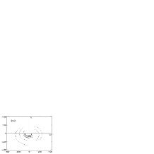
Figure 2: Coverages of the uv-plane of the simulated 10-baseline interferometer related to data formed at 5 (a), 8 (b), 15 (c) and 22 (d) GHz. The axes are in units of millions of wavelengths.

The uv-plane coverages related to a model interferometer consisting of 10 baselines of the VLBA array (BR-LA, BR-MK, BR-NL, BR-PT, BR-OV, BR-SC, BR-KP, BR-HN, BR-FD, LA-MK) and source with a declination $\delta=70\degr$ for each of “observation” frequencies are shown in Fig. 2. Note that the choice of baselines was not principal for our task and was made in an arbitrary way. It was assumed that a duration of the observations is nine hours and visibility data are formed every 30 minutes. As it can be seen, the uv-plane at different frequencies has the same topology but scaled accordingly. As far as interferometer baselines are measured in wavelengths, $u$- and $v$- visibility coordinates are proportional to an observation frequency.

Model maps of the source at frequencies of 5, 8, 15 and 22 GHz are shown in Fig. 3, left column. These maps were obtained from the model map shown in Fig. 1, left, according to the model spectral index distribution (Fig. 1, right) and expression (1) for the spectral dependence. Parameters of the model source intensity maps, such as total flux density ($S_{\rm tot}$), peak flux density ($S_{\rm peak}$) and entropy, are given in Table 1. Comparison of the maps and their parameters shows although not strong but still quite noticeable frequency dependence.

The complex visibility functions, computed in accordance with the Van Cittert-Cernike theorem, consists of 172 samples for each “observation” frequency. Each visibility value was aggravated with additive random error to form data with a typical signal-to-noise ratio of averaged and self-calibrated VLBI data of about 10⁴. It is necessary to emphasize that we do not consider here the selfcalibration problems (Conway, Cornwell & Wilkinson, 1990) and concentrate only on removing spectral errors.

The main goals of the simulation fulfilled were: (i) to show efficiency of the multi-frequency synthesis for improving intensity images in case of small-element interferometers with poor uv-plane filling; (ii) to illustrate the consequences of multi-frequency synthesis without any spectral correction; (iii) to estimate the possibility of reconstruction of spectral index maps with a satisfactory quality.

We performed three tests. The first one was single-frequency synthesis of the source images at 5, 8, 15 and 22 GHz. The second one was multi(four)-frequency synthesis without any spectral correction. And, finally, the third experiment was devoted directly to multi-frequency synthesis with spectral correction, at the reference frequency of 13.6 GHz.

Figure 1: Intensity map for the model radio source at 13.6 GHz (left) and model spectral index map (right). Relative right ascension and declination are given in mas along the horizontal and vertical axes, respectively. Contour levels: 0.2, 0.4, 0.8, 1.6, 3.2, 6.4, 12.8, 25.6, 51.2, 90% of the peak flux density of 0.196 Jy/pixel.

The single-frequency maps are presented in Fig. 3, right column. Their parameters are given in Table 2. Analysis of the results obtained shows the following. The amount of data proves to be too small, and uv-plane filling too poor to obtain images with sufficient quality. Comparison of Table 1 and 2 allows us to judge about distortions of the reconstructed images. As a criterium of the reconstructed image quality, we chose the signal-to-noise ratio (SNR) listed in the last column in Table 2, which was calculated in the following way:

$${\rm SNR}=\frac{\sqrt{\sum_{k,l}I_{\rm mod}^{2}(k,l)}}{\sqrt{\sum_{k,l}(I_{\rm mod}(k,l)-I_{\rm rec}(k,l))^{2}}},$$

where $I_{\rm mod}$ is the model map, $I_{\rm rec}$ is the reconstructed map, $k,l=1,\ldots,N$, where $N$ is the linear size of the map.

As it is seen from the single-frequency maps, at lower observation frequencies, the lower resolution is ensured. The lower-frequency maps show a larger-scale structure, while the higher-frequency maps show smaller-scale features. The highest accuracy of reconstruction is achieved at frequencies of 8 and 15 GHz (${\rm SNR}\sim 16$). At the lowest frequency, 5 GHz, and the highest frequency, 22 GHz, the obtained reconstruction quality was much worse (SNR is about 8).

The uv-plane corresponding to multi(four)-frequency synthesis is presented in Fig. 4, left. The multi-frequency map obtained without any spectral corrections of the frequency-dependent source brightness distribution is shown in Fig. 4, right. Parameters of the synthesized map are given in Table 3. Comparing with the model map (Fig. 1), we can see large image distortions which are reflected in such map parameters as the total flux density, entropy and SNR ($\sim$ 7). Large image distortions in the case of relatively small values of spectral index distribution (Fig. 1, right) can be explained by a wide frequency range of the data.

The intensity map and spectral index image obtained using the multi-frequency synthesis algorithm with spectral correction are shown in Fig. 5. Note that we tried the different numbers of spectral terms in expansion (2). Here we present the results related to utilization of three spectral terms. Further increase in the number of spectral terms did not improve our results substantially. Using fewer spectral terms proved to be insufficient due to the wide frequency range of the data. Having analyzed the results (Fig. 5 and Table 3), we can conclude that taking into account the frequency dependence of the source brightness distribution allowed us to obtain both the source intensity map (${\rm SNR}\sim 36$) and spectral index distribution over the source with high accuracy.

Thus, in the source model with sufficiently complicated extended structure, typical for AGN at milliarcsecond scales, with typical spectral index values, we demonstrated the ability of the MEM-based multi-frequency synthesis algorithm with spectral correction for both (i) improving intensity images and (ii) obtaining spectral index maps of high quality. We emphasize that the use of the MFS algorithm is especially effective in the case of small-element interferometers with poor uv-plane filling. We also showed the consequences of ignoring frequency dependence of the source brightness distribution in multi-frequency synthesis algorithm.

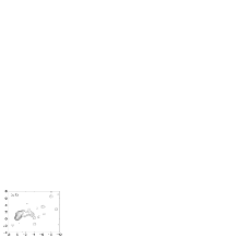
Figure 3: Model (left column) and reconstructed (right column) images at 5 (a), 8 (b), 15 (c) and 22 GHz (d). Relative right ascension and declination are given in mas along the horizontal and vertical axes, respectively. Contour levels: 0.2, 0.4, 0.8, 1.6, 3.2, 6.4, 12.8, 25.6, 51.2, 90% of the peak flux density (see Tables 1 and 2).

Figure 4: Coverage of the uv-plane related to multi(four)-frequency data (left) and the image reconstructed from the four-frequency data ignoring any frequency dependence of the source brightness distribution (right). The $u$- and $v$-axes are in units of millions of wavelengths. Relative right ascension and declination are given in mas along the horizontal and vertical axes, respectively. Contour levels: 0.2, 0.4, 0.8, 1.6, 3.2, 6.4, 12.8, 25.6, 51.2, 90% of the peak flux density of 0.194 Jy/pixel.

Figure 5: Intensity image (left) and spectral index distribution (right) reconstructed from the four-frequency data using the GMEM-based algorithm with spectral correction (reference frequency is 13.6 GHz). Relative right ascension and declination are given in mas along the horizontal and vertical axes, respectively. Contour levels: 0.2, 0.4, 0.8, 1.6, 3.2, 6.4, 12.8, 25.6, 51.2, 90% of the peak flux density of 0.198 Jy/pixel.

Table 2: Parameters of single-frequency reconstructed images.

Frequency	$S_{\rm tot}$	$S_{\rm peak}$	Entropy	SNR
(GHz)	(Jy)	(Jy/pixel)
15.0	5.16	0.168	$-$18.3	17.4
18.4	4.71	0.187	$-$16.1	16.8
15.4	4.54	0.197	$-$15.5	16.5
22.2	4.41	0.189	$-$15.7	18.4

6 The problem of image alignment

One of the most important sources of information about the physical conditions in the radio-emitting regions of AGN is the spectral index distribution over the source. The core region is usually characterized by a large optical depth and an almost flat or inverted spectrum, while the jets are optically thin with respect to synchrotron radiation and have steeper spectra (Croke & Gabuzda, 2008; O’Sullivan & Gabuzda, 2009; Pushkarev et al., 2005).

Table 3: Parameters of four-frequency reconstructed images.

MFS experiment	$S_{\rm tot}$	$S_{\rm peak}$	Entropy	SNR
	(Jy)	(Jy/pixel)
No spectral corr.	5.85	0.194	$-$22.7	17.2
With spectral corr.	4.71	0.198	$-$16.6	36.2

The spectral index distribution over the source can be constructed by various methods. The traditional method suggests: (i) formation of images at two separate frequencies, $\nu_{1}$ and $\nu_{2}$, with the solutions of the deconvolution problem (CLEAN or MEM) being convolved with the same clean beam corresponding to the lower observation frequency; (ii) calculation of the two-dimensional spectral index distribution over the source from equation (1). Obviously, this sequence of operations is legitimate only when the positions of the VLBI cores of sources (not to be confused with the physical core of the source that is undetectable due to absorption effects) are frequency-independent.

The image reconstruction using the iterative selfcalibration procedure is known (Thompson, Moran & Swenson, 2001) to lead to the loss of information about the absolute position of the source on the sky: during the phase self-calibration, the centroid of the object is placed at the phase center of the map with coordinates $(0,0)$. However, since most of the radio-loud AGN are characterized by a dominant compact core (Kovalev et al., 2005; Lister & Homan, 2005; Lee et al., 2008), the VLBI core of the source coincides with the peak radio brightness of the source in an overwhelming majority of cases.

Nevertheless, the standard theory of extragalactic radio sources (Blandford & Königl, 1979) predicts a frequency-dependent VLBI core shift due to opacity effects in the source’s core region. Synchrotron self-absorption takes place in an ultra-compact region near the “central engine” of AGN, the mechanism of which is most efficient at low frequencies. As a result, the apparent origin of the jet manifests itself farther from the physical core along the jet axis at lower frequencies (Fig. 6). This theoretical prediction was confirmed by observations: the frequency-dependent shift in the core position was measured for several quasars by Lobanov (1998). In the literature, this phenomenon is also actively debated from the viewpoint of the accuracy of astrometric measurements (Charlot, 2002; Boboltz, 2006; Kovalev et al., 2008a).

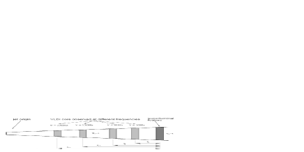
Figure 6: A scheme illustrating the frequency-dependent position shift of the VLBI core (modified from Kovalev et al. (2008a)).

It thus follows that the multi-frequency data analysis must be preceded by the alignment of images at different frequencies. This can be achieved in three ways: (i) performing VLBI observations of the objects under study together with reference sources; (ii) finding the parameters of the shift of one image relative to the other by aligning compact optically thin jet features, which are not subject to absorption effects to the same extent as in the source’s core (Paragi, Fejes & Frey, 2000; Kovalev et al., 2008a); (iii) finding the shift parameters using a cross-correlation analysis (Croke & Gabuzda, 2008). Being laborious from the viewpoint of performing observations and their subsequent reduction, the first method gives no significant advantage in determining the shift and its accuracy; therefore, the second and/or third methods are used more often.

Recall that the alignment procedure implemented by shifting one image relative to the other is equivalent to the phase correction of the spectrum (or visibility function) of the image being shifted relative to the fixed one. The need of precorrecting the data for the source’s visibility function at different frequencies makes the direct use of the multi-frequency synthesis algorithm described above problematic, because the frequency dependence of the core shift is not known in advance. It can be determined by forming the images at each frequency and determining the corresponding shifts. As it was shown by Kovalev et al. (2008b), O’Sullivan & Gabuzda (2009) and Sokolovsky et al. (2011), the frequency dependence of the VLBI core position is well fitted by a hyperbolic dependence of the form $r\propto\nu^{-1}$. Thus, our multi-frequency synthesis procedure can be used after allowance for the shifts in the positions of the VLBI cores at different frequencies and their coordinates relative to the phase center and applying the corresponding frequency-dependent phase corrections to the visibility function.

7 Real data processing. Four-frequency imaging for 0954+658

Here we present the results of applying the developed multi-frequency image synthesis algorithm to the real VLBI data of the extragalactic radio source 0954+658, a member of the complete sample of BL Lacertae objects (Kühr & Schmidt, 1990). Note that 0954+658 is also a member of the 1FGL catalog of $\gamma$-ray bright sources detected by the Large Area Telescope onboard the Fermi observatory and positionally associated with the $\gamma$-ray source 1FGL J1000.1+6539 (Abdo et al., 2010). This source is of our interest because it has a typical parsec-scale morphology that includes an optically thick VLBI core and a one-sided optically thin jet, which is expected to manifest itself in the spectral index distribution. General information on this source is given in Table 4.

Table 4: General parameters of 0954+658.

Other name	Right	Decli-	Opt.	red-	1FGL
	ascension	nation	ID	shift
	(J2000)	(J2000)		($z$)
J0958+6533	9h 58m	$+65\degr 33\arcmin$	BL	0.367	Y
	47.2451s	$54.818\arcsec$	Lac

The VLBA observations of 0954+658 were carried out in a “snapshot” mode in 1997 April (1997.26) simultaneously at four frequencies: 5, 8, 15 and 22 GHz. The data were calibrated in the NRAO AIPS package using standard procedures. The images were formed within the framework of the Pulkovo “VLBImager” software package based on a self-calibration algorithm (Cornwell & Fomalont, 1999) in combination with a GMEM-based deconvolution procedure.

The uv-plane coverages related to the observation frequencies of 5, 8, 15 and 22 GHz are shown in Fig. 7. The MEM-based single-frequency maps are shown in Fig. 8. Parameters of these maps, obtained from the MEM-solutions by convolution with “clean” beams that determine the system’s resolution at each observation frequency, are given in Table 5.

Figure 7: Coverages of the uv-plane at 5 (a), 8 (b), 15 (c) and 22 (d) GHz for VLBA observations of 0954+658. The axes are in units of millions of wavelengths.

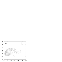
Figure 8: Single-frequency maps of the source 0954+658 reconstructed from the data at 5 (a), 8 (b), 15 (c) and 22 (d) GHz. Relative right ascension and declination are given in mas along the horizontal and vertical axes, respectively. The lowest contour levels are given in Table 5 for each image, the values of the succeeding levels are doubled.

Table 5: Parameters of single-frequency maps for 0954+658.

Freq-	$S_{\mathrm{tot}}$	$S_{\mathrm{peak}}$	Beam	Lowest
uency	mJy	mJy/	FWHM	contour
GHz		beam	mas$\times$mas, PA	level, $\%$
15.0	617	360	2.50$\times$1.72, $-$17$\aas@@fstack{\circ}$3	0.20
18.4	496	311	1.44$\times$1.05, $-$16$\aas@@fstack{\circ}$2	0.10
15.4	454	219	0.81$\times$0.59, $-$16$\aas@@fstack{\circ}$0	0.25
22.2	310	166	0.58$\times$0.43, $-$21$\aas@@fstack{\circ}$6	0.70

The parameters of the frequency-dependent image shift found by aligning compact features of the optically thin jet are given in Table 6. As expected, the direction of the shift coincides with the inner jet orientation. The uv-plane related to the multi(four)-frequency data is shown in Fig. 9, left.

Table 6: Frequency-dependent VLBI core position shifting parameters with respect to the core position at 22 GHz.

Frequency, GHz	$\Delta_{r}$, mas	Position Angle
15.4	0.18	$-$29$\aas@@fstack{\circ}$4
18.4	0.46	$-$27$\aas@@fstack{\circ}$1
15.0	0.73	$-$29$\aas@@fstack{\circ}$7

Figure 9: Coverage of the uv-plane related to multi(four)-frequency data (left) and the image reconstructed from the four-frequency data ignoring any frequency dependence of the source brightness distribution (right). The $u$- and $v$-axes are in units of millions of wavelengths. Relative right ascension and declination are given in mas along the horizontal and vertical axes, respectively. Total VLBA flux density is 434 mJy. Beam FWHM is 0.58$\times$0.43 mas, $\mathrm{PA}=-$21$\aas@@fstack{\circ}$6. Contour levels: 0.2, 0.4, 0.8, 1.6, 3.2, 6.4, 12.8, 25.6, 51.2, 90% of the peak flux density of 179 mJy/beam.

First, we processed the multi-frequency data ignoring dependence of the source brightness distribution on observation frequency. The image obtained is shown in Fig. 9, right. Then we applied our MFS algorithm with spectral correction to the multi-frequency data, but we did not correct the data in accordance with the frequency-dependent VLBI core position shift found. Results of this multi-frequency synthesis obtained at central reference frequency 13.6 GHz are shown in Fig. 10.

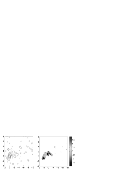
Figure 10: Intensity (left) and spectral index (right) maps reconstructed from the four-frequency data using the GMEM-based algorithm with spectral correction, but without preliminary data correction for frequency-dependent core position shift (reference frequency is 13.6 GHz). Relative right ascension and declination are given in mas along the horizontal and vertical axes, respectively. Total VLBA flux density is 450 mJy. Beam FWHM is 0.58$\times$0.43 mas, $\mathrm{PA}=-$21$\aas@@fstack{\circ}$6. Contour levels: 0.2, 0.4, 0.8, 1.6, 3.2, 6.4, 12.8, 25.6, 51.2, 90% of the peak flux density of 151 mJy/beam.

Finally, we applied our multi-frequency synthesis algorithm with spectral correction to the observational data that were first corrected according to the alignment parameters (Table 6). The image obtained at reference frequency of 13.6 GHz and the corresponding two-dimensional spectral index distribution are shown in Fig. 11.

Figure 11: Intensity (left) and spectral index (right) maps reconstructed from the four-frequency data using the GMEM-based algorithm with spectral correction and preliminary data correction for frequency-dependent core position shift (reference frequency is 13.6 GHz). Relative right ascension and declination are given in mas along the horizontal and vertical axes, respectively. Total VLBA flux density is 496 mJy. Beam FWHM is 0.58$\times$0.43 mas, $\mathrm{PA}=-$21$\aas@@fstack{\circ}$6. Contour levels: 0.2, 0.4, 0.8, 1.6, 3.2, 6.4, 12.8, 25.6, 51.2, 90% of the peak flux density of 189 mJy/beam.

The intensity images shown in Fig. 9, 10 and 11 are obtained by convolving solutions for $I_{0}$ with appropriate gaussian beam. The spectral index images (Fig. 10 and 11) are formed by dividing two solutions for $I_{1}$ and $I_{0}$ in accordance with equation (5) after convolving them with the same beam.

It is necessary to note that the main goal of this section is to demonstrate the necessity of taking into account the frequency-dependent image shift in order to correctly map the spectral index distribution.

Let us analyze the results obtained.

The VLBI structure of the radio source 0954+658 consists of an optically thick core (Fig. 11, right) and an optically thin jet initially extending in the North-West direction up to $\sim 2$ mas from the VLBI core and then turning to the West. As it is seen from single-frequency maps Fig. 8), the apparent extent of the jet reaches about 12 mas and 2 mas at the lowest and the highest frequencies, respectively. Total flux density of the source varies from 0.6 up to 0.3 Jy at the lowest and the highest frequencies, respectively. One can see that the images obtained manifest large-scale structure features at lower observation frequencies and small-scale ones at higher frequencies.

Combining the data obtained at different observation frequencies allows us, in general, to reconstruct both large- and small-scale structures to a larger extent because of a better filled uv-plane. That was proved, in particular, in Section 5 in model experiments.

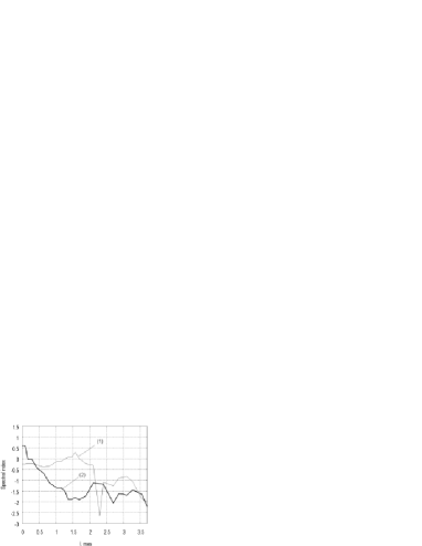
Figure 12: Slices of the spectral index distributions along the jet ridge line beginning from the phase center: (1) and (2) are related to the spectral index maps presented in Fig. 10 and Fig. 11 respectively; $l$ is the distance along the ridge line.

The intensity map (Fig. 9) synthesized directly from the linearly combined multi-frequency data without any spectral corrections shows large source structure distortions and many artifacts. Multi-frequency synthesis with spectral correction, fulfilled first without taking into account frequency-dependent VLBI core position shift, shows a slight improvement of the source intensity map, but it is still distorted, especially in the South-West direction (Fig. 10). But the main consequence of image misalignment is an incorrect reconstruction of the spectral index distribution. In our case we can see that the spectral index map obtained does not correspond to the physical meaning of an optically thick core and an optically thin jet: there are negative spectral indices in the core region and segments with positive spectral indices in the jet region. From Fig. 11, we realize that only allowance for the real shift found by aligning features of the optically thin jet yielded the proper result. As it is seen, we managed to reconstruct a more extended jet structure (up to 8 mas along the RA axis) than in the case of using only the high-frequency data but with the same high angular resolution. The spectral index map adequately reflects the physical characteristics of the regions of the optically thick compact VLBI core and the optically thin extended jet. We see a fairly regular structure with smooth transitions between segments of different intensities along the entire source. For comparison, one-dimensional slices of the spectral index distributions (see Fig. 10, left and Fig. 11, left) obtained along the jet ridge line are shown in Fig. 12, from which we can graphically evaluate undesirable consequences of ignoring the frequency-dependent VLBI core position shift in the MFS algorithm.

8 Conclusions

We developed and tested an efficient multi-frequency image synthesis algorithm with the correction for the frequency dependence of the radio brightness of a source. The algorithm is based on the generalized maximum entropy method; it allows one to take into account the spectral terms of any order and to map both a total intensity image and spectral index distribution, which is of great importance in investigating the physical characteristics of AGN.

The advantage of the proposed multi-frequency synthesis algorithm is that the spectral terms of any order can be easily taken into account in the entropic functional being minimized. This allows for the spectral correction of images to be made both in a wide frequency range and for large spectral indices.

We have shown how important the allowance for the frequency-dependent image shift is in applying the multi-frequency synthesis algorithm. Our conclusions are based on the results of processing the multi-frequency VLBA data for the BL Lac object 0954+658 with a fairly complex extended jet structure, which also manifests itself in the spectral index distribution over the source.

Analysis of the results obtained shows that multi-frequency synthesis is an efficient method for improving the mapping quality; low-frequency data allow the extended structure of a source to be reconstructed more completely, while high-frequency data allow a high spatial resolution to be achieved. It should also be emphasized that the spectral index distribution can be mapped with a high quality as well.

References

- Abdo et al. (2010) Abdo A. A., Ackermann M., Ajello M., Allafort A., Antolini E., Atwood W. B., Axelsson M., Baldini, L., Ballet J., Barbiellini G., et al., 2010, ApJ, 715, 429
- Ables (1974) Ables J. G., 1974, AASS, 15, 383
- Bajkova (1992) Bajkova A. T., 1992, Astron. Astrophys. Trans., 1, 313
- Bajkova (1993) Bajkova A. T., 1993, Reports of IAA RAS, N 58 (in Russian)
- Bajkova (2005) Bajkova A. T., 2005, Astron. Rep., 49, 947
- Bajkova (2007) Bajkova A. T., 2007, Astron. Rep., 51, 891
- Bajkova (2008) Bajkova A. T., 2008, Astron. Rep., 52, 951
- Blandford & Königl (1979) Blandford R. D., Königl A., 1997, APJ, 232, 34
- Boboltz (2006) Boboltz D. A.,2006, IERS Technical Note 34, Intern.l Celest. Reference System and Frame, Verlag des Bundesamtes füur Kartographie and Geodsie, Frankfurt-am-Main
- Charlot (2002) Charlot P., 2002, Proc. of the Intern. VLBI Service for Geodesy and Astrometry 2000, General Meeting, NASA/CP-2002-210002, p. 233
- Conway (1991) Conway J. E., 1991, ASP Conf. Ser., 19, 171