Ballistic (precessional) contribution to the conventional magnetic switching

Abstract

We consider a magnetic moment with an easy axis anisotropy energy, switched by an external field applied along this axis. Additional small, time-independent bias field is applied perpendicular to the axis. It is found that the magnet’s switching time is a non-monotonic function of the rate at which the field is swept from “up” to “down”. Switching time exhibits a minimum at a particular optimal sweep time. This unusual behavior is explained by the admixture of a ballistic (precessional) rotation of the moment caused by the perpendicular bias field in the presence of a variable switching field. We derive analytic expressions for the optimal switching time, and for the entire dependence of the switching time on the field sweep time. The existence of the optimal field sweep time has important implications for the optimization of magnetic memory devices.

In conventional magnetic switching by an externally applied magnetic field the moment performs many revolutions before switching to the opposite direction. While being much slower than the ballistic (precessional) switching back:1999 ; xiao:2006 ; wang:2007 which is tested experimentally but not yet realized in applications, conventional switching is used for magnetic recording in hard disk drives and other devices. The speed at which the moments of magnetic bits can be switched between the two easy directions has obvious implications for the technology performance, setting the limit for the information writing rate. Here we study the dependence of the conventional magnetic switching time $\tau_{m}$ on the reversal time of the writing head field. If the field is swept from “up” to “down” in a time $\tau_{h}$, the switching time will be a function $\tau_{m}(\tau_{h})$. It would seem natural to assume that $\tau_{m}$ decreases with decreasing $\tau_{h}$ and the fastest switching is realized by an instantaneous flip of the field with $\tau_{h}=0$. However, it was found numerically by one of the authors stankiewicz that in the presence of a small perpendicular bias field the function $\tau_{m}(\tau_{h})$ is not monotonic and has a minimum at an optimal sweep time $\tau_{h}^{*}$. Decreasing $\tau_{h}$ below the optimal value would be counterproductive in terms of the technology performance. In this paper we provide analytic approximations for the function $\tau_{m}(\tau_{h})$ and the optimal field sweep time $\tau_{h}^{*}$. We find that the nonmonotonic behavior of $\tau_{m}(\tau_{h})$ is a result of the admixture of a “ballistic” (or “precessional”) switching induced by the perpendicular bias field. Ballistic contribution is normally quenched by the anisotropy, but here it is restored by the time-dependence of the field during the rise time of the applied step. The effect considered here is different from the decrease of the switching time suess:2002 predicted for switching below the Stoner-Wholfarth limit.he:1994 ; porter:1998 The latter consists of the $\tau_{m}$ dependence on the amplitude of the field step with an instantaneous rise time, while in our case the finite rise time is essential. Conventional switching considered here is achieved by a field step and does not require precisely timed pulses of finite duration needed for a truly ballistic switching. back:1999 ; xiao:2006 ; wang:2007 Also, the required field magnitude is much smaller than in the ballistic case.

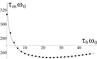
Figure 1: Switching time $\tau_{m}$ as a function of field sweep time $\tau_{h}$. Here $\alpha=0.01$, $h_{0}=3.5\ \omega_{0}$, $h_{\perp}=0.001\ \omega_{0}$. The solid line is given by the analytical expression (1).

Magnetic particles of nanometer size are single-domain back:1999 ; thirion:2003 and can be described by the moment ${\bf M}=M_{0}{\bf n}$, where ${\bf n}$ is a unit vector. We consider a particle with an easy axis $\hat{z}$ and anisotropy energy $E_{a}=-(1/2)Kn_{z}^{2}$. The switching field ${\bf H}=H(t)\hat{z}$ is directed along the easy axis. For large enough field magnitudes, $|H|>K/M_{0}$, only one equilibrium direction of $\bf M$ is stable. A field applied exactly along the axis leads to a magnetization switch only when some fluctuations of $\bf M$ are present. Following Ref. stankiewicz, we introduce a small constant perpendicular bias field ${\bf H}_{\perp}=H_{\perp}\hat{x}$, $H_{\perp}\ll K/M_{0}$ to mimic the required fluctuations.

The dynamics of the moment are governed by the Landau-Lifshitz-Gilbert (LLG) equation

$$\dot{\bf M}=-\gamma\left[\frac{\partial E}{\partial{\bf M}}\times{\bf M}\right]+\frac{\alpha}{M_{0}}[{\bf M}\times\dot{\bf M}]\ ,$$

where $\gamma$ is the gyromagnetic ratio, $E=E_{a}-({\bf H}+{\bf H}_{\perp})\cdot{\bf M}$ is the total magnetic energy, and $\alpha\ll 1$ is the Gilbert damping constant. The field sweep is assumed to be linear in time and given by the expressions $H(t)=+H_{0}$ for $t<0$, $H(t)=H_{0}(1-2t/\tau_{h})$ for $0<t<\tau_{h}$, and $H(t)=-H_{0}$ for $t>\tau_{h}$. As the field is swept from positive to negative values, the up-equilibrium disappears and the magnetic moment starts to move towards the down-equilibrium along a spiral trajectory. The final approach to the down-equilibrium in exponential. To define a finite switching time we have to introduce a provisional cut-off angle $\theta_{sw}$ and calculate the time it takes to reach it. The extra time needed to cover the remaining distance does not depend on $\tau_{h}$ because that part of the motion happens at a constant field $H=-H_{0}$. In accord with Refs. stankiewicz, ; suess:2002, ; he:1994, ; porter:1998, we choose $\theta_{sw}=\pi/2$.

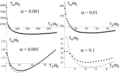
Figure 2: Dependencies $\tau_{m}(\tau_{h})$ calculated for $h_{0}=2.2\ \omega_{0}$, $h_{\perp}=0.001\ \omega_{0}$, and variable $\alpha$ indicated on each panel. As $\alpha$ increases, the theoretical fit gets poorer due to the violation of the strong inequality (4).

The LLG equation can be easily solved numerically and the switching time dependence $\tau_{m}(\tau_{h})$ can be obtained. Fig. 1 shows the results of such modeling for a particular parameter set. The minimum of $\tau_{m}$ is clearly observed.

We have derived an approximate analytic expression for the switching time. Denoting $h_{0}=\gamma H_{0}$, $h_{\perp}=\gamma H_{\perp}$, and $\omega_{0}=\gamma K/M_{0}$ we find

$$\tau_{m} \approx \frac{3h_{0}+\omega_{0}}{4h_{0}}\tau_{h}+\frac{\ln[h_{0}/\pi h_{\perp}^{2}\tau_{h}]}{2\alpha(h_{0}-\omega_{0})}+\tau_{R}\ ,$$ (1)

where $\tau_{R}$ is a part independent of $\tau_{h}$ and $h_{\perp}$

$$\tau_{R} = \frac{1}{2\alpha}\left\{\frac{1}{h_{0}-\omega_{0}}\ln\left(\frac{2(h_{0}-\omega_{0})}{h_{0}}\right)\right.-$$

$$-\left.\frac{1}{h_{0}+\omega_{0}}\ln\left(\frac{h_{0}-\omega_{0}}{2h_{0}}\right)\right\}\ .$$

Formula (1) is the first main result of our paper. As one can see in Fig. 1, it reproduces the function $\tau_{m}(\tau_{h})$ quite well.

Approximation (1) requires small $h_{\perp}$ and $\alpha$. For a given $h_{\perp}$ it is valid in the interval of field sweep times

$$\frac{h_{0}}{(h_{0}-\omega_{0})^{2}}\ll\tau_{h}\ll\tau_{h}^{(+)}\ ,$$ (2)

where $\tau_{h}^{(+)}$ is a solution of

$$\sqrt{\frac{\tau_{h}}{h_{0}}}e^{-\alpha\tau_{h}\frac{(h_{0}-\omega_{0})^{2}}{4h_{0}}}=\frac{1}{h_{\perp}}\ .$$

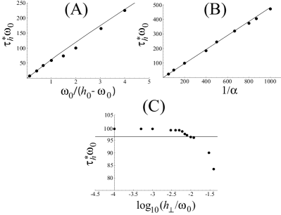
Figure 3: Numeric (points) and approximate analytical (solid lines) dependencies of the optimal field sweep time $\tau_{h}^{*}$ on the system parameters: (a) fixed $\alpha$ and $h_{\perp}$, (b) fixed $h_{0}/\omega_{0}$ and $h_{\perp}$, (c) fixed $h_{0}/\omega_{0}$ and $\alpha$. When not varied, the parameter values are $h_{0}=2.2\omega_{0}$, $\alpha=0.01$, $h_{\perp}=0.005$.

The optimal sweep time $\tau_{h}^{*}$ is determined from $\partial\tau_{m}/\partial\tau_{h}=0$. We get an expression

$$\tau_{h}^{*}=\frac{1}{2\alpha(h_{0}-\omega_{0})}\frac{4h_{0}}{3h_{0}+\omega_{0}}\ .$$ (3)

This formula is our second main result. Note that $\tau_{h}^{*}$ is independent of the bias field. The minimal switching time $\tau_{m}(\tau_{h}^{*})$ itself depends on $h_{\perp}$, which is quite natural since the initial deviation from the easy axis is controlled by $h_{\perp}$. We have also calculated the switching time drop

$$\tau_{m}(0)-\tau_{m}(\tau_{h}^{*})=\frac{\ln\left(\frac{\pi(h_{0}-\omega_{0})(h_{0}+\omega_{0})^{2}}{2\alpha h_{0}^{2}(3h_{0}+\omega_{0})}\right)-1}{2\alpha(h_{0}-\omega_{0})}\ .$$

between the instant and the optimal field sweeps. The drop is independent of the bias field as long as approximation (1) is valid.

Formula (3) is valid when $\tau_{h}^{*}$ falls into the interval (2). Our calculations show that this is guaranteed for

$$\frac{h_{\perp}^{2}}{h_{0}(h_{0}-\omega_{0})}\ll\alpha\ll\frac{h_{0}-\omega_{0}}{2h_{0}}\ .$$ (4)

These inequalities place a more stringent constraint on the Gilbert damping than the simple $\alpha\ll 1$.

Fig. 2 compares numerically calculated switching times with our analytic formula (1). When inequalities (4) are well satisfied, the quality of approximation is very good. As one approaches the limits of the approximation’s validity by, e.g., increasing $\alpha$, the errors grow larger.

Fig. 3 shows the dependence of the optimal field sweep time $\tau_{h}^{*}$ on the system parameters. The correspondence with formula (3) is generally good, although some visible deviations exist. The accuracy of the determination of $\tau_{h}^{*}$ is lowered by a flat shape of the $\tau_{m}(\tau_{h})$ minimum. The shallow minimum, however, also lowers the practical importance of precise determination of $\tau_{h}^{*}$.

In general, the analytic expression can approximate the $\tau_{m}(\tau_{h})$ dependence up to a 10% accuracy in a surprisingly wide range of parameters. Such accuracy is certainly sufficient for the estimates related to the device design.

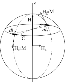
Figure 4: Average “ballistic” contribution of the bias field. Vector ${\bf M}(t)$ orbits around a parallel circle $C$ on a sphere $|{\bf M}|=M_{0}$. The torque due to ${\bf H}_{\perp}$ pushes $\bf M$ along the meridians of the sphere. In constant switching field $\bf H$ the torque contributions from the diametrically opposed elements $dl_{1}$ and $dl_{2}$ cancel each other. For variable ${\bf H}(t)$ such a cancelation does not happen because ${\bf M}$ spends unequal amounts of time on $dl_{1}$ and $dl_{2}$.

We now discuss the physical reason for the minimum of the function $\tau_{m}(\tau_{h})$. The bias field has two roles in the switching process. First, it provides the initial deviation from the easy axis. Second, it alters the equations of motion for ${\bf M}(t)$. The derivation of Eqs. (1) and (3), which will be detailed in our forthcoming paper, shows that the second contribution is dominant. Recall now that in the absence of anisotropy and other fields the torque ${\bf H}_{\perp}\times{\bf M}$ due to the bias field would rotate vector $\bf M$ from $+\hat{z}$ to $-\hat{z}$ along a meridian of the sphere $|{\bf M}|=M_{0}$ (dashed line in Fig. 4), in a ballistic (precessional) fashion. In our case a weak bias field is applied on top of the strong uniaxial anisotropy and switching field, which together induce a fast orbital motion of vector ${\bf M}(t)$ along the parallel circles (line $C$ in Fig. 4). The bias field still attempts to move $\bf M$ along the meridians, but now its action has to be averaged over the orbital period. As illustrated in Fig. 4, in constant fields ${\bf H}=\pm H_{0}\hat{z}$ averaging gives zero due to the cancelation of the contributions from the diametrically opposed infinitesimal intervals $dl_{1}$ and $dl_{2}$ of equal lengths. This way ballistic contribution of the bias field is quenched. However, the contribution of ${\bf H}_{\perp}$ does not average to zero for a variable switching field ${\bf H}(t)$. In this case the velocity of $\bf M$ changes along the orbit, the times spent in the intervals $dl_{1}$ and $dl_{2}$ are different, and the contributions of the two do not cancel each other. We conclude that in the presence of a time dependent external field ${\bf H}(t)$ ballistic contribution of the perpendicular bias field is recovered. Moreover, this contribution helps to move vector $\bf M$ from $+\hat{z}$ to $-\hat{z}$ and is thus responsible for the initial decrease of $\tau_{m}$. As the sweep time grows larger, the change of the orbital velocity during the precession period decreases and the ballistic contribution averages out progressively better. The helping effect of ballistic switching is lost and $\tau_{m}$ starts to increase as it normally would.

Ballistic contribution to switching can be also viewed as a phenomenon complimentary to the magnetic resonance and rf-assisted switching,thirion:2003 ; bertotti:2001 ; rivkin:2006 where ${\bf H}$ is constant but ${\bf H}_{\perp}(t)$ is time-dependent. There the average contribution of the bias field on an orbit does not vanish due to the time dependence of ${\bf H}_{\perp}$. The non-vanishing contribution, regardless of its origin, assists the switching and makes it faster.

Our analytical results provide a convenient approximation for the optimal field sweep time, an important parameter in the device design. They can be used as a starting point for the investigations of the switching time in granular media, where each grain can be modeled by a single moment and bias fields are produced by the other grains or by the spread of grain orientations.

Ya. B. Bazaliy is grateful to B. V. Bazaliy for illuminating discussions. This work was supported by the NSF grant DMR-0847159.

References

- (1) C. H. Back, R. Allenspach, W. Weber, S. S. P. Parkin, D. Weller, E. L. Garwin, and H. C. Siegmann, Science 285, 864 (1999).
- (2) Di Xiao, M. Tsoi, and Qian Niu, J. Appl. Phys. 99, 013903 (2006).
- (3) X. R. Wang and Z. Z. Sun, Phys. Rev. Lett. 98, 077201 (2007).
- (4) A. Stankiewicz, APS March Meeting, Portland, OR, March 15-19, 2010. Bulletin of the APS 55(2), abstract H33.11.
- (5) D. Suess, T. Schrefl, W. Scholz, and J. Fidler, J. Magn. Magn. Mater. 242-245, 426 (2002).
- (6) L. He, W. D. Doyle, and H. Fujiwara, IEEE Trans. Magn. 30, 4086 (1994).
- (7) D. G. Porter, IEEE Trans. Magn. 34, 1663 (1998).
- (8) C. Thirion, W. Wernsdorfer, and D. Mailly, Nat. Mater. 2, 524 (2003).
- (9) G. Bertotti, C. Serpico, and I. D. Mayergoyz, Phys. Rev. Lett. 86, 724 (2001).
- (10) K. Rivkin and J. B. Ketterson, Appl. Phys. Lett. 89, 252507 (2006).