Moving walls accelerate mixing

Abstract

Mixing in viscous fluids is challenging, but chaotic advection in principle allows efficient mixing. In the best possible scenario, the decay rate of the concentration profile of a passive scalar should be exponential in time. In practice, several authors have found that the no-slip boundary condition at the walls of a vessel can slow down mixing considerably, turning an exponential decay into a power law. This slowdown affects the whole mixing region, and not just the vicinity of the wall. The reason is that when the chaotic mixing region extends to the wall, a separatrix connects to it. The approach to the wall along that separatrix is polynomial in time and dominates the long-time decay. However, if the walls are moved or rotated, closed orbits appear, separated from the central mixing region by a hyperbolic fixed point with a homoclinic orbit. The long-time approach to the fixed point is exponential, so an overall exponential decay is recovered, albeit with a thin unmixed region near the wall.

I Introduction

In many engineering applications, a viscous fluid must be blended with a substance, referred to as a passive scalar. This is generally called mixing, and it is well known that stirring greatly enhances this process. In fact, even if turbulence is unavailable (because of low Reynolds number or delicate substances), it is possible to mix rapidly by the process of chaotic advection Aref (1984); Ottino (1989). This involves the chaotic stretching of fluid particles by the flow, and the subsequent increase in concentration gradients of the substance to be mixed. The increased gradients facilitate the action of molecular diffusion, and homogeneity ensues. The net process (chaotic advection together with diffusion) is known as chaotic mixing.

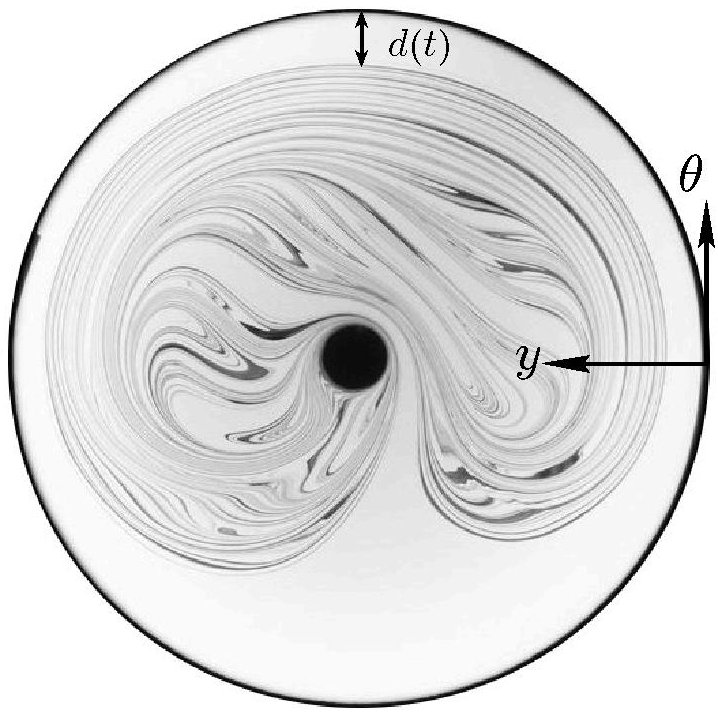
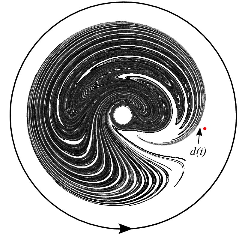
Figure 1: (a) Experiment with the ‘figure-eight’ stirring protocol, showing an advected blob of dye (India ink) in sugar syrup (details of the experimental apparatus are given in Gouillart et al. (2007, 2008)). The coordinate system used here is also indicated, as is the distance $d(t)$ between the dark mixing pattern and the distinguished parabolic point on the wall. See Fig. 2 for the rod’s path. (b) Numerical simulation for the same stirring protocol as in (a), but with the wall rotating at a rate $\Omega=0.4\ \mathrm{rad/s}$. Here, $d(t)$ is the distance from the mixing pattern to the hyperbolic point indicated by a dot.

The quantity that is often tracked in mixing problems is the variance of the concentration of the scalar Danckwerts (1952); Rothstein et al. (1999); Jullien et al. (2000); Fereday et al. (2002); Sukhatme and Pierrehumbert (2002); Voth et al. (2003); Villermaux and Duplat (2003); Thiffeault and Childress (2003). The variance is the spatial integral of the squared deviation from the mean concentration, and measures therefore the intensity of concentration fluctuations. The reasoning is that the variance tends to zero as the concentration is homogenized. Simple arguments Zeldovich et al. (1984); Shraiman and Siggia (1994); Antonsen, Jr. et al. (1996); Balkovsky and Fouxon (1999); Fereday et al. (2002); Thiffeault and Childress (2003); Thiffeault (2008); Haynes and Vanneste (2005); Meunier and Villermaux (2010) suggest that the concentration variance should decay exponentially with time. In an idealized scenario the fluid particles are stretched exponentially and folded by the flow, yielding a characteristic filamentary structure as in Fig. 1. The filaments then achieves an equilibrium width where diffusion balances stretching Batchelor (1959). Subsequently, the concentration field for that particle decays exponentially at the rate of stretching. An average over rates of stretching then gives the overall decay rate of the variance. In many cases the decay rate of the variance is determined in a less local manner Pierrehumbert (1994); Fereday et al. (2002); Wonhas and Vassilicos (2002); Pikovsky and Popovych (2003); Fereday and Haynes (2004); Thiffeault and Childress (2003); Haynes and Vanneste (2005), but the decay is still exponential.

This basic exponential-decay picture is appealing, but it is complicated by the presence of walls. In that case, several authors Jones and Young (1994); Chertkov and Lebedev (2003); Lebedev and Turitsyn (2004); Schekochihin et al. (2004); Salman and Haynes (2007); Popovych et al. (2007); Chernykh and Lebedev (2008); Mackay (2008); Boffetta et al. (2009); Zaggout and Gilbert (2011) have suggested that the no-slip boundary condition and the presence of separatrices on the walls slow down mixing: the decay rate is algebraic rather than exponential. Recent experiments Gouillart et al. (2007, 2008, 2009) have confirmed this, and also showed that for a significant period of time the rate of decay of variance is dramatically reduced, even away from the walls, due to the entrainment of unmixed material into the central mixing region.

In this paper, which is a more detailed and complete exposition of an earlier letter Gouillart et al. (2010), we show that if the situation is such that mixing is slowed down by no-slip walls, then this can be cured by moving the wall in such a way as to destroy the separatrices. This creates closed orbits near the wall, effectively insulating the central mixing region from the wall (see Fig. 2). The rate of decay of the concentration variance becomes exponential rather than algebraic. The price to pay is that the thin region of closed orbits remains poorly mixed. Of course, in some applications moving or spinning the outer wall of a container is not practical, so we also discuss other mechanisms for creating closed orbits near the wall.

The outline of the paper is as follows. In Section II we analyze the case of a device consisting of a stirring rod and a fixed outer wall. We describe the separatrices that appear at the boundary, and how the approach along the stable manifold of one of these separatrices is algebraic in time. In Section III we treat the same system, but with the wall rotating at a constant velocity. We find the wall separatrices are destroyed; instead, a hyperbolic fixed point appears away from the wall, with a homoclinic orbit separating the wall region from the central mixing region. The approach along the stable manifold of that fixed point is exponential in time.

Section IV relates these results to the decay of concentration variance. We show that if the wall is rotating fast enough, the decay rate is not limited by the no-slip boundary condition, and mixing proceeds as rapidly as it would in the absence of a no-slip wall. We present numerical evidence for this in Section V, based on simulations of the evolution of the concentration field for a simple, but realistic, flow. We then offer some concluding remarks, and discuss other ways of creating closed orbits beyond physically rotating the wall.

II Fixed Wall

Consider the experiment for the time-periodic ‘figure-eight’ rod-stirring protocol shown in Fig. 1. The numerically-computed Poincaré section

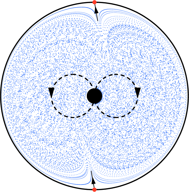
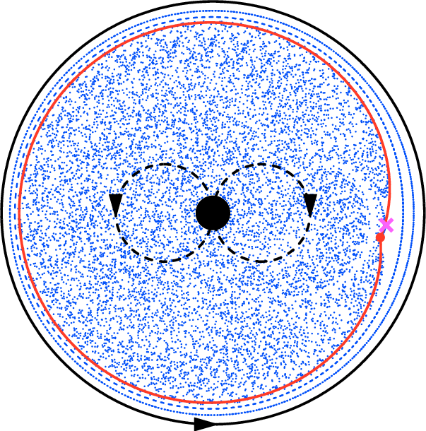
Figure 2: (a) Numerical Poincaré section (stroboscopic map) of a single trajectory for the time-periodic figure-eight stirring protocol (dashed line). The circular domain has unit radius, the rod has radius $0.08$, and the rod’s two circular paths have radius $0.23$. The chaotic region covers the entire domain, all the way to the wall, where two near-wall separatrices are indicated in the upper and lower portions of the domain. (b) Same parameters, but with the outer wall rotating at a rate of $\Omega=0.2$ radians per period. Closed orbits appear near the wall, and the wall separatrices are destroyed. There is however a separatrix associated with a hyperbolic fixed point of the map (solid line), which isolates the chaotic region from the wall. The solid dot is the approximate position of the fixed point according to the model in Section III, and the cross is the numerically-measured fixed point. The discrepancy can easily be resolved by expanding to next order in $\Omega$.

for the same 2-D Stokes flow (Fig. 2) shows that this protocol promotes chaotic advection in the whole domain, as could be expected from the stretching and folding of dye filaments visible in Fig. 1. It also shows clearly that particles move very slowly near the wall, as evidenced by the closely-packed successive iterates, in accordance with the no-slip boundary condition. This suggests writing the flow near the wall as a simple map,

$$\bar{}\theta=\theta+A(\theta)y+\mathrm{O}\!\left(y^{2}\right),\qquad\bar{}y=y-\tfrac{1}{2}A^{\prime}(\theta)y^{2}+\mathrm{O}\!\left(y^{3}\right).$$ (1)

where $(\theta,y)$ is the position of a fluid particle at the beginning of a time interval, $(\bar{}\theta,\bar{}y)$ its new position at the end. Here $\theta$ is an angle measured counterclockwise along the wall, and $0\leq y\ll 1$ measures the distance from the wall (Fig. 1). The first equation in (1) uses continuity and the no-slip boundary condition at the wall; then the second equation follows from incompressibility and the no-throughflow condition at the wall. The container is assumed to have unit radius. We can write $(\theta,y)=(\theta(t),y(t))$ and $(\bar{}\theta,\bar{}y)=(\theta(t+T),y(t+T))$, where $t$ is time, $T$ is the period, and $t/T$ is the number of full periods of the stirring protocol that the system has undergone. If we truncate the map by neglecting the higher-order terms, then it preserves area only to first order in $y$. We shall see in Section III how to correct the map to ensure exact area preservation.

Since it is continuous, the tangential velocity near the wall can only reverse sign at points $\theta$ with $A(\theta)=0$. These points correspond to the upper and lower wall separatrices (also called separation and reattachment points) visible in Fig. 2. (Note that these only act as separatrices near the wall, where the flow is almost steady; further away from the wall the manifolds of the separation points take a more convoluted form that permits chaotic transport in the bulk of the vessel.) There are only two such separatrices, so we conclude that $A(\theta)$ must be as in Fig. 3, with the two zeros

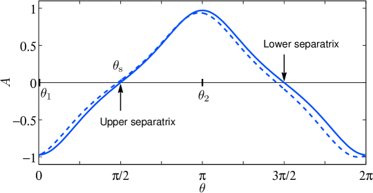
Figure 3: Solid line: The periodic function $A(\theta)$ in Eq. (1) for the figure-eight stirring motion of Fig. 2. The two zeros correspond to the separatrices connected to the wall at the points highlighted in Fig. 2. The upper (stable) separatrix is at $\theta=\theta_{\mathrm{s}}=\pi/2$, and the lower (unstable) separatrix is at $\theta=3\pi/2$. The dashed line is for the same stirring motion, but with the wall rotating at angular velocity $\Omega=0.2$ per stirring period.

corresponding to the separatrices in Fig. 2. (The functions in Fig. 3 were obtained numerically from 2D Stokes flow simulations Finn et al. (2003).)

Every point $(\theta,y)=(\theta_{0},0)$ on the wall is a fixed point of the map (1). Letting $(\theta,y)=(\theta_{0}+\Theta,0+Y)$, where $(\Theta,Y)$ are small expansion variables, we find the dynamics of particle trajectories near that point,

$$\overline{\Theta} =\Theta+A(\theta_{0})Y+A^{\prime}(\theta_{0})\Theta Y+\mathrm{O}\!\left(\Theta^{2}Y\,,\,Y^{2}\right),$$ (2a)

$$\overline{Y} =Y-\tfrac{1}{2}A^{\prime}(\theta_{0})Y^{2}+\mathrm{O}\!\left(\Theta Y^{2}\,,\,Y^{3}\right).$$ (2b)

The eigenvalues associated with the linearization of (2) are both unity, so $(\theta_{0},0)$ is a distinguished parabolic fixed point Reichl (2004). Near most of these points the dynamics are uninteresting: particles just stream along the wall following $\overline{\Theta}=\Theta+A(\theta_{0})Y$, and approach or recede from the wall depending on the sign of $A^{\prime}(\theta_{0})$. Eventually we must give up using (2), since the trajectories always leave the neighborhood of $(\theta_{0},0)$. However, for the two values of $\theta$ for which $A(\theta)$ vanishes (see Fig. 3), we get separatrices near the wall.

We focus on the separatrix at $\theta=\theta_{\mathrm{s}}=\pi/2$, where $A(\theta_{\mathrm{s}})=0$, and Eqs. (2) become

$$\overline{\Theta} =\Theta+A^{\prime}(\theta_{\mathrm{s}})\Theta Y+\mathrm{O}\!\left(\Theta^{2}Y\,,\,Y^{2}\right),$$ (3a)

$$\overline{Y} =Y-\tfrac{1}{2}A^{\prime}(\theta_{\mathrm{s}})Y^{2}+\mathrm{O}\!\left(\Theta Y^{2}\,,\,Y^{3}\right),$$ (3b)

with $(\theta,y)=(\theta_{\mathrm{s}}+\Theta,0+Y)$ and $(\Theta,Y)$ small expansion variables. Now the set $\{\Theta=0,Y>0\}$ is invariant for small $Y$ and corresponds to the separatrix, which is the stable manifold of the fixed point $(\theta_{\mathrm{s}},0)$. The evolution along the stable manifold is obtained by iterating

$$\overline{Y}=Y-\tfrac{1}{2}A^{\prime}(\theta_{\mathrm{s}})Y^{2},$$ (4)

for small $Y$. This is a logistic map, and as we approach the fixed point at $Y=0$ we expect $Y$ to change very little at each period. This suggests writing (4) as a differential equation for $Y(t)$,

$$\frac{\overline{Y}-Y}{T}\simeq\dot{}Y=-\tfrac{1}{2T}A^{\prime}(\theta_{\mathrm{s}})Y^{2},\qquad{(\overline{Y}-Y)}/{T}\ll 1.$$ (5)

The overdot denotes a time derivative. The solution is

$$Y(t)=\frac{Y(0)}{1+\tfrac{1}{2}A^{\prime}(\theta_{\mathrm{s}})Y(0)(t/T)}\,.$$ (6)

For this to represent the stable manifold, we require $A^{\prime}(\theta_{\mathrm{s}})>0$, as is clear from Fig. 3. (The other separatrix exhibits finite-time escape to infinity, which takes particles away from the wall and into the bulk.) For long times, the rate of approach is

$$Y(t)\sim\frac{2}{A^{\prime}(\theta_{\mathrm{s}})}\,(t/T)^{-1}\,,\qquad t/T\gg(\tfrac{1}{2}A^{\prime}(\theta_{\mathrm{s}})Y(0))^{-1}\,.$$ (7)

The asymptotic form (7) for $Y(t)$ is algebraic and independent of $Y(0)$. The consequence of this independence is visible in the upper part of Fig. 1: material lines ‘bunch-up’ against each other faster than they approach the wall, thereby forgetting their initial position.

The slow algebraic approach to the wall exhibited in (7) was shown in Gouillart et al. (2007, 2008, 2009) to cause a drastic slowdown of the overall mixing rate in the vessel. Indeed, even though the fundamental action of the stirring protocol is chaotic, as evident in Fig. 2, a pool of unmixed fluid remains near the wall for very long times. More importantly, this pool contaminates the entire mixing pattern, all the way to its core, as unmixed fluid leaks slowly along the unstable manifold of the separation point at $\theta=3\pi/2$, resulting in the characteristic cusped shape of the dye pattern in Fig. 1. This is because there is no barrier between the wall and the central mixing region. In the next section, we will see how we can create such a barrier by moving the outer wall.

III Moving Wall

Now we consider the case of a slowly-rotating wall, with mixing pattern as in Fig. 1. The near-wall map corresponding to (1) is

$$\bar{}\theta=\theta+\Omega+A(\theta)y,\qquad\bar{}y=y-\tfrac{1}{2}A^{\prime}(\theta)y^{2},$$ (8)

where $0<\Omega\ll 1$ is the angular displacement of the wall per period, and we have neglected higher-order terms in $y$. We assume that $\Omega$ is small since in that case $A(\theta)$ will change little from the case with $\Omega=0$, as can be seen by the dashed line in Fig. 3.

To help understand how the velocity $\Omega$ modifies the wall map, it is instructive to plot iterates for a specific form of $A(\theta)$. To match the numerical simulations, $A(\theta)$ must be periodic in $\theta$ and have only two zeros (Fig. 3); a simple model is then to take $A(\theta)=-\cos\theta$. For plotting iterates, it is preferable to use the exact area-preserving version of (8) (see Appendix A),

$$\bar{}\theta=\theta+\Omega+A(\theta)\bar{}y,\qquad\bar{}y=y-\tfrac{1}{2}A^{\prime}(\theta)\bar{}y^{2},$$ (9)

which has unit Jacobian. (Using the exact map guarantees a faithful representation of closed orbits; but note that $(\theta,y)$ are only approximate canonical variables, for small $y$.) Figure 4 shows trajectories for the map (9). Once a particle leaves the vicinity of the wall, its trajectory becomes meaningless, since our expansions (1) and (8) are only valid for small $y$. However, the cusp structure for $\Omega=0$ in Fig. 4 is evident and is remarkably similar to the lower part of Fig. 1, where the unstable separatrix is located.

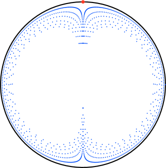
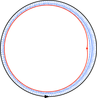
Figure 4: Iterates the area-preserving near-wall map map (9), which should be compared to the full numerical simulations of Fig. 2. (a) $\Omega=0$, with the upper stable distinguished parabolic fixed point shown as a dot; (b) $\Omega=0.2$, with the hyperbolic fixed point shown as a dot, and its associated homoclinic separatrix plotted as a solid line. We can clearly see closed trajectories outside the separatrix, near the wall. Once trajectories leave the vicinity of the wall, Eq. (9) no longer applies and we must look into the specific stirring mechanism.

Now we analyze the map (8) as we did in Section II when the wall was fixed. Again we look for fixed points of (8). All the distinguished parabolic fixed points on the wall have disappeared, as well as the two separatrices. Since $A(\theta)$ is continuous, has two zeros, and $A^{\prime}(\theta_{\mathrm{s}})>0$, $A(\theta)$ must have a minimum at $\theta_{1}$ and a maximum at $\theta_{2}$, where $A^{\prime}(\theta_{1,2})=0$ and hence $\bar{}y(\theta_{1,2},y)=y$ for all $y$. Seeking values for which the along-wall velocity also vanishes, we find there are fixed points at $y_{1,2}=-\Omega/A(\theta_{1,2})$, which we require to be small for our analysis (that is, this defines how slow the rotation has to be). Since $A(\theta_{2})>0$ (maximum) and $A(\theta_{1})<0$ (minimum), only $\theta_{1}$ has $y_{1}\geq 0$. (Recall that we assume $\Omega>0$.) The other fixed point lies outside our domain. Hence, we focus on the unique near-wall fixed point $(\theta_{1},-\Omega/A(\theta_{1}))$. (There could be others if $A(\theta)$ has more extrema, but here we restrict to the case of two extrema.)

We look at the linearized dynamics near the fixed point. Let $(\theta,y)=(\theta_{1}+\Theta,-\Omega/A(\theta_{1})+Y)$; then

$$\overline{\Theta} =\Theta+A(\theta_{1})Y+\mathrm{O}\!\left(\Theta^{2},Y^{2},\Theta Y\right),$$ (10a)

$$\overline{Y} =Y-\tfrac{1}{2}A^{\prime\prime}(\theta_{1})y_{1}^{2}\,\Theta+\mathrm{O}\!\left(\Theta^{2},Y^{2},\Theta Y\right).$$ (10b)

To leading order in $\Theta$ and $Y$, the motion near the fixed point is thus described by

$$\begin{pmatrix}\overline{\Theta}\\ \overline{Y}\end{pmatrix}=\begin{pmatrix}1&A(\theta_{1})\\ -\tfrac{1}{2}A^{\prime\prime}(\theta_{1})y_{1}^{2}&1\end{pmatrix}\begin{pmatrix}\Theta\\ Y\end{pmatrix}.$$ (11)

The matrix in the above equation has eigenvalues

$$\mu_{\pm}=1\pm\sqrt{-\tfrac{1}{2}A(\theta_{1})A^{\prime\prime}(\theta_{1})}\,y_{1}=1\pm\sqrt{-\frac{A^{\prime\prime}(\theta_{1})}{2A(\theta_{1})}}\,\Omega$$ (12)

where the argument in the square root is nonnegative since $A(\theta_{1})<0$ and $A^{\prime\prime}(\theta_{1})\geq 0$. For $A^{\prime\prime}(\theta_{1})>0$ and $\Omega>0$, this is a hyperbolic fixed point, and the approach along its stable manifold obeys

$$Y(t)\sim Y(0)\,\exp(-\mu\,t/T)$$ (13)

for $(\Theta(0),Y(0))$ initially on the stable manifold, with decay rate

$$\mu=\sqrt{-\tfrac{1}{2}A(\theta_{1})A^{\prime\prime}(\theta_{1})}\,y_{1}=\sqrt{-\frac{A^{\prime\prime}(\theta_{1})}{2A(\theta_{1})}}\,\Omega$$ (14)

to first order in $\Omega$. Compare this to (7): the approach to the fixed point is now exponential, at a rate proportional to the speed of rotation of the wall. In Fig. 5 we show the results for $\mu$ based on Eq. (14) and as measured in numerical simulations such as in Fig. 2. The two agree for small $\Omega$, as expected. In Section IV, we will see that the rate of exponential decay given by $\mu$ will dominate if it is slower than the mixing rate in the bulk. Otherwise, if $\mu$ is large enough, then the rate of mixing in the bulk dominates.

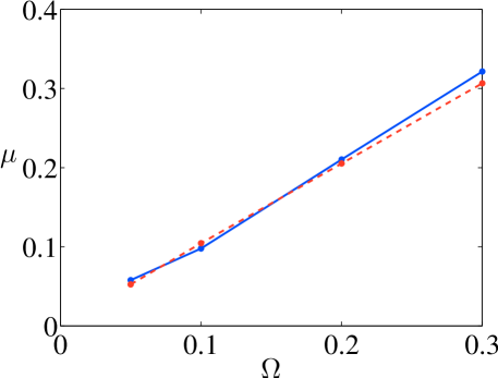
Figure 5: The decay rate to the fixed point $\mu$ measured from simulations (solid line) and from Eq. (14). The two converge to each other for small $\Omega$.

Figure 2 shows a Poincaré section for $\Omega=0.2$. Very close to the wall (within a distance proportional to $\Omega$) trajectories are closed. A separatrix, consisting of a homoclinic orbit connecting the hyperbolic fixed point to itself, isolates the wall region from the bulk. Now it is the approach to this separatrix that will limit the decay rate, and as given by Eq. (13) this approach is exponential. Since the iterates of the map are close together on the separatrix, we can find an equation for the separatrix by writing a stream function

$$\psi(\theta,y)=\tfrac{1}{2}A(\theta)y^{2}+\Omega y\,,\qquad(u,v)=(\partial_{y}\psi\,,\,-\partial_{\theta}\psi)$$ (15)

for a steady flow corresponding to the map. The value of the stream function at the hyperbolic fixed point is $\psi(\theta_{1},-\Omega/A(\theta_{1}))=-\tfrac{1}{2}\Omega^{2}/A(\theta_{1})$. The separatrix thus satisfies

$$\tfrac{1}{2}A(\theta)y_{\text{s}}^{2}(\theta)+\Omega y_{\text{s}}(\theta)=-\tfrac{1}{2}\Omega^{2}/A(\theta_{1})\,,$$ (16)

which we can solve for $y_{\text{s}}(\theta)$,

$$y_{\text{s}}(\theta)=\Omega\,\frac{-1+\sqrt{1-A(\theta)/A(\theta_{1})}}{A(\theta)}=y_{1}\,\frac{1-\sqrt{1-A(\theta)/A(\theta_{1})}}{A(\theta)/A(\theta_{1})}\,.$$ (17)

where we have chosen the solution of the quadratic that ensures $y_{\text{s}}(\theta)>0$. The argument of the square root is always positive, since $\theta_{1}$ is a global minimum and $A(\theta_{1})<0$. When $\theta=\theta_{1}$ we recover $y_{\text{s}}(\theta_{1})=y_{1}$, as required. The singularity when $A(\theta)=0$ is removable, and we have then $y_{\text{s}}=\tfrac{1}{2}y_{1}$. The distance from the separatrix to the wall is proportional to $\Omega$; the point of closest approach to the wall is at $\theta_{2}$ where $A(\theta)$ is maximum, and the farthest from the wall is at $\theta_{1}$ where $A(\theta)$ is minimum (the hyperbolic fixed point itself). Figure 2 shows the separatrix and fixed point, computed using the theory in this section from the observed $A(\theta)$ for a moving wall (see Fig. 3, dashed line). The separatrix clearly divides the chaotic sea from the wall region. The cross in Fig. 2 is the numerically-computed fixed point for the map. The discrepancy between the numerical value and the theory is due to $\Omega$ being relatively large in this figure ($\Omega=0.2$), and can be easily accounted for by expanding to next order in $\Omega$.

IV Decay of Variance

So far in Sections II and III we have shown the following: (i) If the wall is not rotating, then there is a distinguished parabolic fixed point at the wall with a stable separatrix; the rate of approach of trajectories along that separatrix is algebraic. (ii) If the wall is rotating, the distinguished parabolic fixed point is destroyed, and instead a hyperbolic fixed point appears elsewhere, away from the wall; the rate of approach of trajectories along the stable manifold of that fixed point is exponential. We shall now show that the different rates of approach are reflected in a different time-evolution for the scalar variance.

The key is that the kidney-shaped ‘mixing pattern,’ by which we mean the shape of a blob that has been advected for several periods of the protocol approaches the fixed point at a rate $d(t)$, where

$$d(t)=\begin{cases}2T/(A^{\prime}(\theta_{\mathrm{s}})\,t),\qquad&\text{fixed wall [Eq.~{}\eqref{eq:asympara}]};\\ d(0)\,{\mathrm{e}}^{-\mu t/T},\qquad&\text{moving wall [Eq.~{}\eqref{eq:asymhyper}]}.\end{cases}$$ (18)

(See Fig. 1 for the definition of $d(t)$.) Indeed, a typical fluid particle first approaches the fixed point before being swept away along the wall or along the separatrix.

Inside the central mixing region, we assume the action of the flow is that of a simple chaotic mixer. By this we mean that fluid elements are stretched, on average, at an exponential rate $\lambda$. For simplicity, we also assume that in the absence of walls the concentration variance decays at the same ‘natural’ decay rate $\lambda$, though in general the two rates can differ Antonsen, Jr. et al. (1996); Balkovsky and Fouxon (1999); Thiffeault (2008); Meunier and Villermaux (2010). Hence, after a time $t$ a typical blob of initial size $\delta$ will have length $\delta\,{\mathrm{e}}^{\lambda t}$. However, because of diffusion, its width will stabilize at an equilibrium between compression and diffusion at the Batchelor scale Batchelor (1959); Balkovsky and Fouxon (1999); Villermaux and Duplat (2003); Thiffeault (2008)

$$\ell_{\mathrm{B}}=\sqrt{\kappa/\lambda},$$ (19)

where $\kappa$ is the molecular diffusivity.

At every period, the pattern gets progressively closer to the wall. Assuming molecular diffusion can be neglected, area preservation implies that some white fluid must have entered the central mixing region. It does so in the form of white strips, clearly visible as layers inside the pattern of Fig. 1. In fact, if we assume that the mixing pattern grows uniformly, we can write the width $\Delta(t)$ of a strip injected at period $t/T$ as

$$\Delta(t)=d(t)-d(t+T)\simeq-T\,{\dot{d\mkern 8.0mu}\mkern-8.0mu}{}(t)$$ (20)

where we also assumed that $d(t)$ changes little at each period, consistent with experimental observations. This is positive since $d$ is a decreasing function of time.

Now, if a white strip is injected at time $\tau<t$, how long does it survive before it is wiped out by diffusion? The answer is the solution to the equation

$$\Delta(\tau)\,{\mathrm{e}}^{-\lambda(t-\tau)}=\ell_{\mathrm{B}}\,.$$ (21)

We interpret this formula as follows: The strip initially has width $\Delta(\tau)$ when it is injected; it is then compressed by the flow in the central mixing region by a factor ${\mathrm{e}}^{-\lambda(t-\tau)}$ depending on its age, $t-\tau$; and once it is compressed to the Batchelor length $\ell_{\mathrm{B}}$ it quickly diffuses away. Thus, we can solve (21) to find the age of a strip when it gets wiped out by diffusion,

$$t-\tau=\lambda^{-1}\log(\Delta(\tau)/\ell_{\mathrm{B}}).$$ (22)

Eventually, at time $t_{\mathrm{B}}$, a newly-injected filament will have width equal to the Batchelor length. This occurs when

$$\Delta(t_{\mathrm{B}})=\ell_{\mathrm{B}},$$ (23)

which can be solved for $t_{\mathrm{B}}$ given a form for $\Delta(t)$. After this time it makes no sense to speak of newly-injected filaments as ‘white,’ since they are already dominated by diffusion at their birth. Hence, the description we present here is valid only for times earlier than $t_{\mathrm{B}}$, but large enough that the edge of the mixing pattern has reached the vicinity of the wall.

In the experiment we measure the intensity of pixels in the central mixing region. We observe for $1\ll t/T\lesssim t_{\mathrm{B}}/T$ that the concentration variance is dominated by the amount of strips in the central region that are still white Gouillart et al. (2007, 2008). Because of area conservation, the total area of injected white material that is still visible at time $t$ is proportional to

$$\mathcal{A}_{\mathrm{w}}(t)=d(\tau(t))-d(t)$$ (24)

where we use (22) to solve for $\tau(t)$, the injection time of the oldest strip that is still white at time $t$. Hence, our goal is to estimate $\mathcal{A}_{\mathrm{w}}(t)$ for times $1\ll t/T\lesssim t_{\mathrm{B}}/T$, since $\mathcal{A}_{\mathrm{w}}$ is directly proportional to the concentration variance. To do this we need $\tau(t)$, which requires specifying $\Delta(t)$. We examine the two possible forms in Eq. (18) in Sections IV.1 and IV.2.

IV.1 Fixed Wall

For the fixed wall of Section II, we have from (18) $d(t)=2T/(A^{\prime}(\theta_{\mathrm{s}})\,t)$. The total area of remaining white strips at time $t$ as given by (24) is proportional to

$$\mathcal{A}_{\mathrm{w}}(t)=\frac{2T}{A^{\prime}(\theta_{\mathrm{s}})\tau}-\frac{2T}{A^{\prime}(\theta_{\mathrm{s}})t}=\frac{2T}{A^{\prime}(\theta_{\mathrm{s}})}\,\frac{t-\tau}{\tau t}\,.$$ (25)

From (18) and (20), the width of injected strips is $\Delta(t)=-T{\dot{d\mkern 8.0mu}\mkern-8.0mu}{}=2T^{2}/(A^{\prime}(\theta_{\mathrm{s}})t^{2})$. Equation (22) cannot be solved exactly, but since $\tau(t)$ is algebraic the right-hand side of (22) is not large, implying that $t/\tau\simeq 1$ for large $t$. We can thus replace $\tau$ by $t$ in (22) and the denominator of (25), and find

$$\mathcal{A}_{\mathrm{w}}(t)\simeq\frac{2T}{A^{\prime}(\theta_{\mathrm{s}})}\,\frac{\log(\Delta(t)/\ell_{\mathrm{B}})}{\lambda\,t^{2}}\,,\qquad 1\ll t/T\lesssim t_{\mathrm{B}}/T.$$ (26)

The decay of concentration variance is algebraic ($\sim 1/t^{2}$), with a logarithmic correction. The form (26) has been verified in experiments and using a simple map model Gouillart et al. (2007, 2008).

IV.2 Moving Wall

Now consider the case of a moving wall, with $d(t)=d(0)\,{\mathrm{e}}^{-\mu t}$ from Eq. (18). We have $\Delta(t)=-T{\dot{d\mkern 8.0mu}\mkern-8.0mu}{}=\mu Td(0)\,{\mathrm{e}}^{-\mu t}=\Delta(0)\,{\mathrm{e}}^{-\mu t}$. From (23), we have $t_{\mathrm{B}}=\mu^{-1}\log(\Delta(0)/\ell_{\mathrm{B}})$, and from (22),

$$t-\tau=\frac{\mu}{\lambda-\mu}\,(t_{\mathrm{B}}-t).$$ (27)

By assumption, $\tau<t<t_{\mathrm{B}}$, so for consistency we require $\mu<\lambda$, i.e., the rate of approach toward the hyperbolic fixed point is slower than the natural decay rate of the chaotic mixer. The area of white material in the mixing region is then obtained from (24),

$$\mathcal{A}_{\mathrm{w}}(t)=d(0)\,{\mathrm{e}}^{-\mu t}\left(\exp\left(\frac{\mu^{2}}{\lambda-\mu}(t_{\mathrm{B}}-t)\right)-1\right),$$ (28)

which in the regime $\lambda/\mu\gg 1$ can be approximated by

$$\mathcal{A}_{\mathrm{w}}(t)\sim d(0)\,\lambda^{-1}\mu^{2}\,(t_{\mathrm{B}}-t)\,{\mathrm{e}}^{-\mu t},\qquad t\lesssim t_{\mathrm{B}}.$$ (29)

The decay rate of the ‘white’ area is completely dominated by the rate of approach to the hyperbolic fixed point. The central mixing process is potentially more efficient ($\lambda>\mu$), but it is starved by the boundaries. Hence, the wall slows down mixing, but unlike the fixed wall (Section IV.1) the decay rate is still exponential.

If the wall rotates rapidly enough to make $\mu>\lambda$, then the wall does not limit the decay rate at all. Indeed, for $\mu>\lambda$, we have $t>t_{\mathrm{B}}$ in (27), since newly injected strips reach the Batchelor length $\ell_{\mathrm{B}}$ before strips that were injected previously. This violates our assumptions, and we conclude that in that case the white strips can be neglected; the decay rate of the concentration variance is then given by the natural decay rate $\lambda$.

In summary, we expect the variance decay rate to be given by

$$\alpha=\min(\mu\,,\lambda),$$ (30)

that is, the decay rate of the variance is given by either the rate of approach to the hyperbolic fixed point $\mu$, or the ‘natural’ decay rate $\lambda$, whichever is slowest. Because the decay rate is always limited by the natural decay rate $\lambda$, one should not rotate the wall faster than is necessary to reach $\mu\sim\lambda$, as further increasing the rotation rate only decreases the size of the chaotic region, without any improvement to the mixing rate. We will see in the next section how this compares to simulations.

V Simulation Results and Discussion

The case of an algebraic decay was well-documented in Gouillart et al. (2007, 2008, 2009), so we focus here on the exponential decay for a moving wall. Figure 6 shows the evolution of variance for several angular rotation rates $\Omega$.

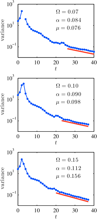
Figure 6: Evolution of variance as a function of period, for different values of the rotation rate $\Omega$. $\alpha$ is the fitted asymptotic decay rate (solid line). For small $\Omega$, $\alpha$ tends to $\mu$ — the decay rate onto the hyperbolic fixed point (see Eq. (14)). (The variance is measured over a finite subregion of the domain, which means it can increase at early times; the break in the top figure is due to an accidental absence of any particles in our measurement region, before particles get mixed.)

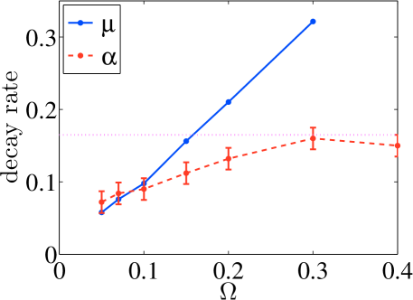
Figure 7: Rate of approach to the fixed point $\mu$ (solid line) and rate of decay of variance $\alpha$ (dashed line).

The variance was obtained by evolving a large number (of order 4 million) of particles to model the concentration field of a passive scalar. This coarse method does not allow us to evolve the concentration field for a long time before particle statistics become inadequate, but we can conclude that the system enters an exponential regime for $t/T\gtrsim 25$, with a rate of decay $\alpha$.

Figure 7 shows the numerically-measured decay rate $\mu$ to the hyperbolic fixed point near the wall (solid line), and the decay rate of the concentration variance (dashed line with error bars). For small $\Omega$, the exponential rate of decay is approximately equal to $\mu$; for larger $\Omega$ it is less than $\mu$, since the decay rate is no longer dominated by the approach to the hyperbolic fixed point. In fact, as predicted by the theory, as the rotation rate is increased the decay rate tends to its “natural” value, approximated here by the dotted line. For small rotation rates, the agreement between $\mu$ and $\alpha$ cannot be called convincing, but is at least consistent. This is partly due to difficulties in measuring the decay rate accurately, as reflected by the large error bars on the dashed line. Note also that the effect is rather small here, so for this particular system the decay rate is not greatly limited by the walls. Nevertheless, we argue that the effect is there, and that in other situations this might be a more significant factor. For instance, it is known that the motion of walls can enhance heat transfer El Omari and Le Guer (2009, 2010).

Evidence that this type of effect could be important is provided by Figs. 8 and 9.

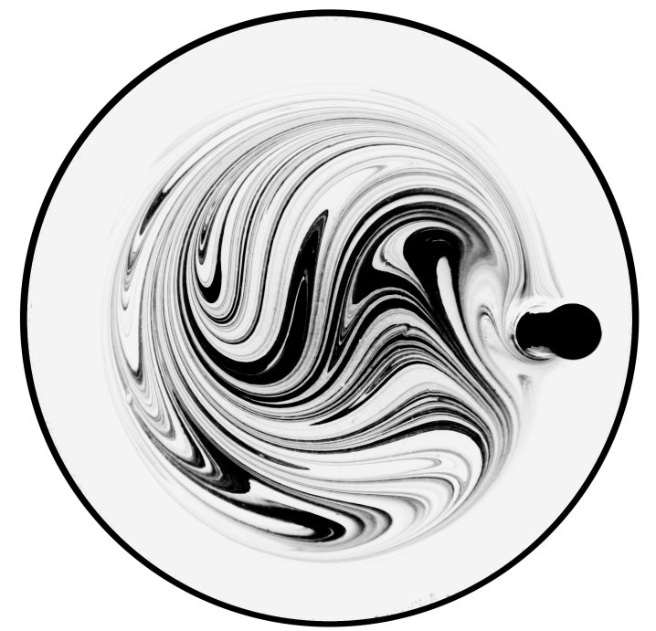
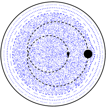
Figure 8: The ‘epitrochoid’ stirring protocol. (a) Experiment; (b) Poincaré section, also showing the rod’s trajectory. Notice the presence of closed orbits near the wall, even though the wall is fixed.

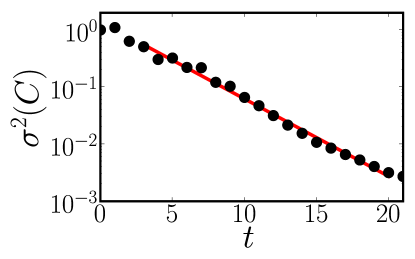
Figure 9: Decay of concentration variance for the epitrochoid stirring protocol (Fig. 8), exhibiting an exponential decay.

They show the results of an experiment where the rod is moved along a “double-loop” rather than the figure-eight (see also Thiffeault et al. (2008) for a discussion of this system). The wall is fixed. Many industrial mixers, for example the wide class of planetary mixers Finn and Cox (2001); Clifford et al. (2004), impose such a multi-loop motion to paddles or stirrers. The double-loop motion, unlike the figure-eight, induces a net angular displacement of particles near the wall, leading to closed orbits (Fig. 8). These closed orbits provide a similar effect to a moving wall: they prevent separatrices from being connected to the wall. Hence, the decay of concentration variance should be exponential, which is confirmed by the experimental results in Fig. 9. The analysis of such a system, however, is significantly harder than the moving wall case presented here. (Note that these two cases are not simply related by changing to a rotating frame: in general the rotation frequency of the wall and the period of the rods are not rationally related, so a fixed frame does not exist.) A detailed study of this case along the lines described here would certainly shed some light on the transition from algebraic to exponential decay, and how system parameters could be tuned for improved mixing efficiency.

Another important generalization is to extend the analysis to three dimensions, where even steady flows can exhibit exponential decay. This is particularly important for microfluidics applications Stroock et al. (2002); Villermaux et al. (2008), where the walls play an important role. The same analysis of separatrices at the walls should carry through, albeit with a richer range of possibilities that is inherent to three dimensions.

Acknowledgments

The authors thank Matthew D. Finn for the use of his computer code for simulating viscous flows, and an anonymous referee for suggesting the area-preserving form of the map in the appendix. J-LT was also partially supported by the Division of Mathematical Sciences of the US National Science Foundation, under grant DMS-0806821.

Appendix A Area-preserving Maps

The near-wall maps (1) and (8) were derived by assuming a simple Taylor expansion in the vicinity of the wall, and applying boundary conditions. However, maps suffer from some drawbacks: they do not exactly preserve area, and they do not satisfy a natural time-reversibility formula. Though these drawback do not quantitatively modify the predictions of the paper, for completeness in this appendix we remedy the situtation.

We wish to derive a symplectic (area-preserving) map for the flow having Hamiltonian (streamfunction)

$$H(\theta,y,t)=\omega y+\tfrac{1}{2}a(\theta)y^{2}\sum_{k=-\infty}^{\infty}\delta(t-kT).$$ (31)

In this flow the fluid near the wall is rotated and ‘kicked’ at each period. The second term in (31) is a perturbation of the integrable first term. Following Abdullaev (2006), the simplest way to obtain an area-preserving map from (31) is to introduce the generating function

$$F(\theta,\bar{}y)=(\theta+\Omega)\bar{}y+\tfrac{1}{2}A(\bar{}\theta)\bar{}y^{2},$$ (32)

with $A(\theta)=a(\theta)T$ and $\Omega=\omega T$. With this type of generating function the mapping $(\theta,y)\rightarrow(\bar{}\theta,\bar{}y)$ is defined implicitly via

$$\bar{}\theta=\frac{\partial F(\theta,\bar{}y)}{\partial\bar{}y},\qquad y=\frac{\partial F(\theta,\bar{}y)}{\partial\theta},$$ (33)

which gives the map

$$\bar{}\theta=\theta+\Omega+A(\theta)\bar{}y,\qquad\bar{}y=y-\tfrac{1}{2}A^{\prime}(\theta)\bar{}y^{2}.$$ (34)

Note that this map is the same as (8) to leading order in $y$. However, unlike (8) it exactly preserves area, by construction. One can see this directly from the generating function $F(\theta,\bar{}y)=F(\theta,\bar{}y(\theta,y))$: from the second equation of (33), we have

$$\frac{\partial y}{\partial\theta}=0=F_{\theta\theta}+F_{\theta\bar{}y}\frac{\partial\bar{}y}{\partial\theta}\quad\Longleftrightarrow\quad\frac{\partial\bar{}y}{\partial\theta}=-\frac{F_{\theta\theta}}{F_{\theta\bar{}y}},$$ (35)

as well as

$$\frac{\partial y}{\partial y}=1=F_{\theta\bar{}y}\frac{\partial\bar{}y}{\partial y}\quad\Longleftrightarrow\quad\frac{\partial\bar{}y}{\partial y}=\frac{1}{F_{\theta\bar{}y}}.$$ (36)

From the first equation of (33), we have

$$\frac{\partial\bar{}\theta}{\partial\theta}=F_{\bar{}y\theta}\frac{\partial\theta}{\partial\theta}+F_{\bar{}y\bar{}y}\frac{\partial\bar{}y}{\partial\theta}=F_{\theta\bar{}y}-\frac{F_{\theta\theta}F_{\bar{}y\bar{}y}}{F_{\theta\bar{}y}},$$ (37)

as well as

$$\frac{\partial\bar{}\theta}{\partial y}=F_{\bar{}y\bar{}y}\frac{\partial\bar{}y}{\partial y}=\frac{F_{\bar{}y\bar{}y}}{F_{\theta\bar{}y}}.$$ (38)

Assembling all this, we find the linearization matrix

$$\frac{\partial(\bar{}\theta,\bar{}y)}{\partial(\theta,y)}=\frac{1}{F_{\theta\bar{}y}}\begin{pmatrix}F_{\theta\bar{}y}^{2}-F_{\theta\theta}F_{\bar{}y\bar{}y}&F_{\bar{}y\bar{}y}\\ -F_{\theta\theta}&1\end{pmatrix}$$ (39)

which always has unit determinant, as required for area preservation. The area-preserving map (34) can be written in explicit form by solving for $\bar{}y$ in the second equation,

$$\bar{}y=\left(\sqrt{1+2A^{\prime}(\theta)y}-1\right)/A^{\prime}(\theta)\,,$$ (40)

where the sign of the quadratic solution was chosen so that the map reduces to (8) for small $y$.

The map (34) solves one of the issues mentioned at the outset: it exactly preserves area. However, it fails to resolve the second issue, time-reversal symmetry. Indeed, interchanging $(\theta,y)$ with $(\bar{}\theta,\bar{}y)$ and letting $T\rightarrow-T$ in (34) leads to a different form for the map, which should not be the case for a map arising from a Hamiltonian such as (31). To fix this is more complicated and requires the introduction of auxiliary variables $(\vartheta,\Upsilon)$ Abdullaev (2006). We quote the form of the resulting map here for completeness:

$$\Upsilon=y-\tfrac{1}{4}A^{\prime}(\theta)\Upsilon^{2},\qquad\vartheta=\theta+\tfrac{1}{2}A(\theta)\Upsilon,$$ (41a)

$$\bar{}\theta=\bar{\vartheta}+\tfrac{1}{2}A(\bar{}\theta)\Upsilon,\qquad\bar{}y=\Upsilon-\tfrac{1}{4}A^{\prime}(\bar{}\theta)\Upsilon^{2},\qquad\bar{\vartheta}=\vartheta+\Omega.$$ (41b)

This map is both area-preserving and invariant under interchange of the barred variables together with $T\rightarrow-T$ (the latter is equivalent to $A\rightarrow-A$ and $\Omega\rightarrow-\Omega$). We can eliminate the $\Upsilon$ and $\vartheta$ auxiliary variables in (41) by solving for $\Upsilon$,

$$\Upsilon=2\left(\sqrt{1+A^{\prime}(\theta)y}-1\right)/A^{\prime}(\theta)\,,$$ (42)

but the first equation in (41b) must still be solved for $\bar{}\theta$, usually numerically.

References

- Aref (1984) H. Aref, ‘Stirring by chaotic advection,’ J. Fluid Mech. 143, 1–21 (1984).
- Ottino (1989) J. M. Ottino, The Kinematics of Mixing: Stretching, Chaos, and Transport (Cambridge University Press, Cambridge, U.K., 1989).
- Gouillart et al. (2007) E. Gouillart, N. Kuncio, O. Dauchot, B. Dubrulle, S. Roux, and J.-L. Thiffeault, ‘Walls inhibit chaotic mixing,’ Phys. Rev. Lett. 99, 114501 (2007).
- Gouillart et al. (2008) E. Gouillart, O. Dauchot, B. Dubrulle, S. Roux, and J.-L. Thiffeault, ‘Slow decay of concentration variance due to no-slip walls in chaotic mixing,’ Phys. Rev. E 78, 026211 (2008), eprint http://arxiv.org/abs/0803.0709.
- Danckwerts (1952) P. V. Danckwerts, ‘The definition and measurement of some characteristics of mixtures,’ Appl. Sci. Res. A A3, 279–296 (1952).
- Rothstein et al. (1999) D. Rothstein, E. Henry, and J. P. Gollub, ‘Persistent patterns in transient chaotic fluid mixing,’ Nature 401 (6755), 770–772 (1999).
- Jullien et al. (2000) M.-C. Jullien, P. Castiglione, and P. Tabeling, ‘Experimental observation of batchelor dispersion of passive tracers,’ Phys. Rev. Lett. 85, 3636 (2000).
- Fereday et al. (2002) D. R. Fereday, P. H. Haynes, A. Wonhas, and J. C. Vassilicos, ‘Scalar variance decay in chaotic advection and Batchelor-regime turbulence,’ Phys. Rev. E 65 (3), 035301(R) (2002).
- Sukhatme and Pierrehumbert (2002) J. Sukhatme and R. T. Pierrehumbert, ‘Decay of passive scalars under the action of single scale smooth velocity fields in bounded two-dimensional domains: From non-self-similar probability distribution functions to self-similar eigenmodes,’ Phys. Rev. E 66, 056302 (2002).
- Voth et al. (2003) G. A. Voth, T. C. Saint, G. Dobler, and J. P. Gollub, ‘Mixing rates and symmetry breaking in two-dimensional chaotic flow,’ Phys. Fluids 15 (9), 2560–2566 (2003).
- Villermaux and Duplat (2003) E. Villermaux and J. Duplat, ‘Mixing as an aggregation process,’ Phys. Rev. Lett. 91, 184501 (2003).
- Thiffeault and Childress (2003) J.-L. Thiffeault and S. Childress, ‘Chaotic mixing in a torus map,’ Chaos 13 (2), 502–507 (2003).
- Zeldovich et al. (1984) Y. B. Zeldovich, A. A. Ruzmaikin, S. A. Molchanov, and D. D. Sokoloff, ‘Kinematic dynamo problem in a linear velocity field,’ J. Fluid Mech. 144, 1–11 (1984).
- Shraiman and Siggia (1994) B. I. Shraiman and E. D. Siggia, ‘Lagrangian path integrals and fluctuations in random flow,’ Phys. Rev. E 49 (4), 2912–2927 (1994).
- Antonsen, Jr. et al. (1996) T. M. Antonsen, Jr., Z. Fan, E. Ott, and E. Garcia-Lopez, ‘The role of chaotic orbits in the determination of power spectra,’ Phys. Fluids 8 (11), 3094–3104 (1996).
- Balkovsky and Fouxon (1999) E. Balkovsky and A. Fouxon, ‘Universal long-time properties of Lagrangian statistics in the Batchelor regime and their application to the passive scalar problem,’ Phys. Rev. E 60 (4), 4164–4174 (1999).
- Thiffeault (2008) J.-L. Thiffeault, ‘Scalar decay in chaotic mixing,’ in J. B. Weiss and A. Provenzale, eds., Transport and Mixing in Geophysical Flows, Lecture Notes in Physics, volume 744, 3–35 (Springer, Berlin, 2008), eprint arXiv:nlin/0502011.
- Haynes and Vanneste (2005) P. H. Haynes and J. Vanneste, ‘What controls the decay of passive scalars in smooth flows?’ Phys. Fluids 17, 097103 (2005).
- Meunier and Villermaux (2010) P. Meunier and E. Villermaux, ‘The diffusive strip method for scalar mixing in two dimensions,’ J. Fluid Mech. 662, 134–172 (2010).
- Batchelor (1959) G. K. Batchelor, ‘Small-scale variation of convected quantities like temperature in turbulent fluid: Part 1. General discussion and the case of small conductivity,’ J. Fluid Mech. 5, 113–133 (1959).
- Pierrehumbert (1994) R. T. Pierrehumbert, ‘Tracer microstructure in the large-eddy dominated regime,’ Chaos Solitons Fractals 4 (6), 1091–1110 (1994).
- Wonhas and Vassilicos (2002) A. Wonhas and J. C. Vassilicos, ‘Mixing in fully chaotic flows,’ Phys. Rev. E 66, 051205 (2002).
- Pikovsky and Popovych (2003) A. Pikovsky and O. Popovych, ‘Persistent patterns in deterministic mixing flows,’ Europhys. Lett. 61, 625–631 (2003).
- Fereday and Haynes (2004) D. R. Fereday and P. H. Haynes, ‘Scalar decay in two-dimensional chaotic advection and Batchelor-regime turbulence,’ Phys. Fluids 16 (12), 4359–4370 (2004).
- Jones and Young (1994) S. W. Jones and W. R. Young, ‘Shear dispersion and anomalous diffusion by chaotic advection,’ J. Fluid Mech. 280, 149–172 (1994).
- Chertkov and Lebedev (2003) M. Chertkov and V. Lebedev, ‘Decay of scalar turbulence revisited,’ Phys. Rev. Lett. 90 (3), 034501 (2003).
- Lebedev and Turitsyn (2004) V. V. Lebedev and K. S. Turitsyn, ‘Passive scalar evolution in peripheral regions,’ Phys. Rev. E 69, 036301 (2004).
- Schekochihin et al. (2004) A. A. Schekochihin, P. H. Haynes, and S. C. Cowley, ‘Diffusion of passive scalar in a finite-scale random flow,’ Phys. Rev. E 70, 046304 (2004).
- Salman and Haynes (2007) H. Salman and P. H. Haynes, ‘A numerical study of passive scalar evolution in peripheral regions,’ Phys. Fluids 19, 067101 (2007).
- Popovych et al. (2007) O. V. Popovych, A. Pikovsky, and B. Eckhardt, ‘Abnormal mixing of passive scalars in chaotic flows,’ Phys. Rev. E 75, 036308 (2007).
- Chernykh and Lebedev (2008) A. Chernykh and V. Lebedev, ‘Passive scalar structures in peripheral regions of random flows,’ JETP Lett. 87 (12), 682–686 (2008).
- Mackay (2008) R. S. Mackay, ‘A steady mixing flow with no-slip boundaries,’ in C. Chandre, X. Leoncini, and G. Zaslavsky, eds., Chaos, Complexity, and Transport: Theory and Applications, 55–68 (World Scientific, Singapore, 2008).
- Boffetta et al. (2009) G. Boffetta, F. De Lillo, and A. Mazzino, ‘Peripheral mixing of passive scalar at small Reynolds number,’ J. Fluid Mech. 624, 151–158 (2009), eprint arXiv:0811.4519.
- Zaggout and Gilbert (2011) F. A. Zaggout and A. D. Gilbert, ‘Passive scalar decay in chaotic flows with boundaries,’ (2011), preprint.
- Gouillart et al. (2009) E. Gouillart, O. Dauchot, J.-L. Thiffeault, and S. Roux, ‘Open-flow mixing: Experimental evidence for strange eigenmodes,’ Phys. Fluids 21 (2), 022603 (2009).
- Gouillart et al. (2010) E. Gouillart, J.-L. Thiffeault, and O. Dauchot, ‘Rotation shields chaotic mixing regions from no-slip walls,’ Phys. Rev. Lett. 104 (20), 204502 (2010).
- Finn et al. (2003) M. D. Finn, S. M. Cox, and H. M. Byrne, ‘Topological chaos in inviscid and viscous mixers,’ J. Fluid Mech. 493, 345–361 (2003).
- Reichl (2004) L. E. Reichl, The Transition to Chaos: Conservative Classical Systems and Quantum Manifestations, second edition (Springer, New York, 2004).
- El Omari and Le Guer (2009) K. El Omari and Y. Le Guer, ‘Numerical study of thermal chaotic mixing in a two rod rotating mixer,’ Comput. Therm. Sci. 1 (1), 55–73 (2009).
- El Omari and Le Guer (2010) K. El Omari and Y. Le Guer, ‘Alternate rotating walls for thermal chaotic mixing,’ Int. J. Heat Mass Transfer 53 (1-3), 123–134 (2010).
- Thiffeault et al. (2008) J.-L. Thiffeault, M. D. Finn, E. Gouillart, and T. Hall, ‘Topology of chaotic mixing patterns,’ Chaos 18, 033123 (2008), eprint arXiv:0804.2520.
- Finn and Cox (2001) M. D. Finn and S. M. Cox, ‘Stokes flow in a mixer with changing geometry,’ J. Eng. Math. 41 (1), 75–99 (2001).
- Clifford et al. (2004) M. J. Clifford, S. M. Cox, and M. D. Finn, ‘Reynolds number effects in a simple planetary mixer,’ Chem. Eng. Sci. 59 (16), 3371–3379 (2004).
- Stroock et al. (2002) A. D. Stroock, S. K. W. Dertinger, A. Ajdari, I. Mezić, H. A. Stone, and G. M. Whitesides, ‘Chaotic mixer for microchannels,’ Science 295, 647–651 (2002).
- Villermaux et al. (2008) E. Villermaux, A. D. Stroock, and H. A. Stone, ‘Bridging kinematics and concentration content in a chaotic micromixer,’ Phys. Rev. E 77 (1), 15301 (2008).
- Abdullaev (2006) S. S. Abdullaev, Construction of Mappings for Hamiltonian Systems and Their Applications, Lecture Notes in Physics, volume 691 (Springer, Berlin, 2006).