Rosetta-Alice Observations of Exospheric Hydrogen and Oxygen on Mars
Abstract
The European Space Agency’s Rosetta spacecraft, en route to a 2014 encounter with comet 67P/Churyumov-Gerasimenko, made a gravity assist swing-by of Mars on 25 February 2007, closest approach being at 01:54 UT. The Alice instrument on board Rosetta, a lightweight far-ultraviolet imaging spectrograph optimized for in situ cometary spectroscopy in the 750–2000 Å spectral band, was used to study the daytime Mars upper atmosphere including emissions from exospheric hydrogen and oxygen. Offset pointing, obtained five hours before closest approach, enabled us to detect and map the HI Lyman- and Lyman- emissions from exospheric hydrogen out beyond 30,000 km from the planet’s center. These data are fit with a Chamberlain exospheric model from which we derive the hydrogen density at the 200 km exobase and the H escape flux. The results are comparable to those found from the the Ultraviolet Spectrometer experiment on the Mariner 6 and 7 fly-bys of Mars in 1969. Atomic oxygen emission at 1304 Å is detected at altitudes of 400 to 1000 km above the limb during limb scans shortly after closest approach. However, the derived oxygen scale height is not consistent with recent models of oxygen escape based on the production of suprathermal oxygen atoms by the dissociative recombination of O.
keywords:
Mars , Mars atmosphere , Atmospheres, evolution1 Introduction
The extended atomic hydrogen corona of Mars was first detected by the ultraviolet spectrometer experiments on the Mariner 6 and 7 spacecraft that measured resonantly scattered solar Lyman- radiation (Barth et al., 1971) to a planetocentric distance of 24,000 km. This was followed by a similar experiment on the orbiting Mariner 9 mission (Barth et al., 1972). Anderson and Hord (1971), using radiative transfer theory, analyzed the early data to derive a hydrogen escape rate, which they found to be compatible with the water photodissociation rate at Mars. Barth et al. (1972) recognized that the apparently constant H escape rate derived from Mariner 6, 7, and 9, if extended backward over geological time scales, would result in an oxygen abundance in the lower atmosphere several orders of magnitude larger than observed. McElroy (1972) suggested that dissociative recombination of O, the dominant ion in the atmosphere, would produce oxygen atoms with sufficient energy to escape. However, since the energetic oxygen atoms are mostly produced below the exobase, determination of the escaping fraction requires detailed modeling, represented by the recent work of Lammer et al. (2003), Fox and Hać (2009), Shematovich et al. (2007), Valeille et al. (2009, 2010), and others. Barth et al. (1971) also reported observations of O i 1304 emission up to 700 km. These data, together with those from Mariner 9, were interpreted by Strickland et al. (1973) in terms of a cool, optically thick oxygen exosphere. Since then, the only measurement of exospheric oxygen on Mars is from the SPICAM instrument on Mars Express (Chaufray et al., 2009), but those data extended only up to 400 km where radiative transfer effects in the O i 1304 multiplet are significant and the evidence for a hot component of O atoms was inconclusive.
Until recently there have also been no additional measurements of the extended hydrogen atmosphere on Mars. Chaufray et al. (2008), again with SPICAM, have measured H i Lyman- emission at 1216 Å, but only up to 4,000 km. Again, they find that a two temperature H exosphere is possible, although the result is inconclusive. Clarke et al. (2009) also suggest a two-component H distribution from monochromatic Lyman- images of Mars showing the H corona out to 4 Mars radii () taken by the Solar Blind Channel of the Advanced Camera for Surveys on HST. Radiative transfer modeling is necessary to extract densities from both of these data sets. Clarke et al. also noted a variation in the Lyman- brightness over a period of two months which they ascribe to a seasonal variation in the H2O loss rate.
We report here on observations of both the extended hydrogen and oxygen coronae of Mars made with the Alice far-ultraviolet imaging spectrograph (Stern et al., 2007) on Rosetta during the spacecraft’s gravity assist swing-by of Mars on 25 February 2007. Offset exposures enabled us to detect and map the H i Lyman- and Lyman- emissions to beyond 30,000 km from the planet’s center. Moreover, except near the planet’s limb, the Lyman- emission is optically thin, allowing us to use a spherical Chamberlain model to determine the temperature and density of H at the exobase without the need for radiative transfer modeling. From limb pointings at spacecraft distances closer to the planet, oxygen emission above the exobase is detected, allowing us to constrain the density of hot oxygen without the need for radiative transfer modeling. These data can be used to derive atomic escape rates and address the question of stoichiometric loss of water vapor from Mars.
2 Observations
Rosetta approached Mars from the day side making its closest approach (CA) at 01:54 UT on 25 February 2007 at an altitude of 250 km. In order to satisfy the scientific goals of the various remote sensing instruments (see, e.g., Coradini, 2010), the common instrument boresight was programmed for a number of fixed pointings towards both the sunlit and dark hemispheres of Mars and offset from Mars, as well as raster scans across the sunlit limb. Due to operational constraints, observations were not possible during the immediate CA period. The pointings of interest in this paper (denoted by the operational designation ALxx) were AL03 pre-CA, centered on the sunlit disk, AL10E, offset pointings centered 2.5∘ and 7.5∘ from Mars along the equator, and AL11B, scans across the illuminated crescent post-CA. Observation start times and geometry parameters are given in Table 1. At the time of closest approach, Mars was 1.445 AU from the Sun and the areocentric longitude, , was 189.9∘. Solar activity was very low for an extended time, including when Earth faced the same solar longitude 9 days earlier, with 72 at 1 AU.
Alice is a lightweight, low-power, imaging spectrograph optimized for in situ cometary far-ultraviolet (FUV) spectroscopy. It is designed to obtain spatially-resolved spectra in the 750-2000 Å spectral band with a spectral resolution between 8 and and 12 Å for extended sources that fill its field-of-view. The slit is in the shape of a dog bone, 5.5∘ long, with a width of 0.05∘ in the central 2.0∘ while the ends are 0.10∘ wide. Each spatial pixel along the slit is 0.30∘. Alice employs an off-axis telescope feeding a 0.15-m normal incidence Rowland circle spectrograph with a concave holographic reflection grating. The imaging microchannel plate detector utilizes dual solar-blind opaque photocathodes (KBr and CsI) and employs a two-dimensional delay-line readout. Details of the instrument are given by Stern et al. (2007).
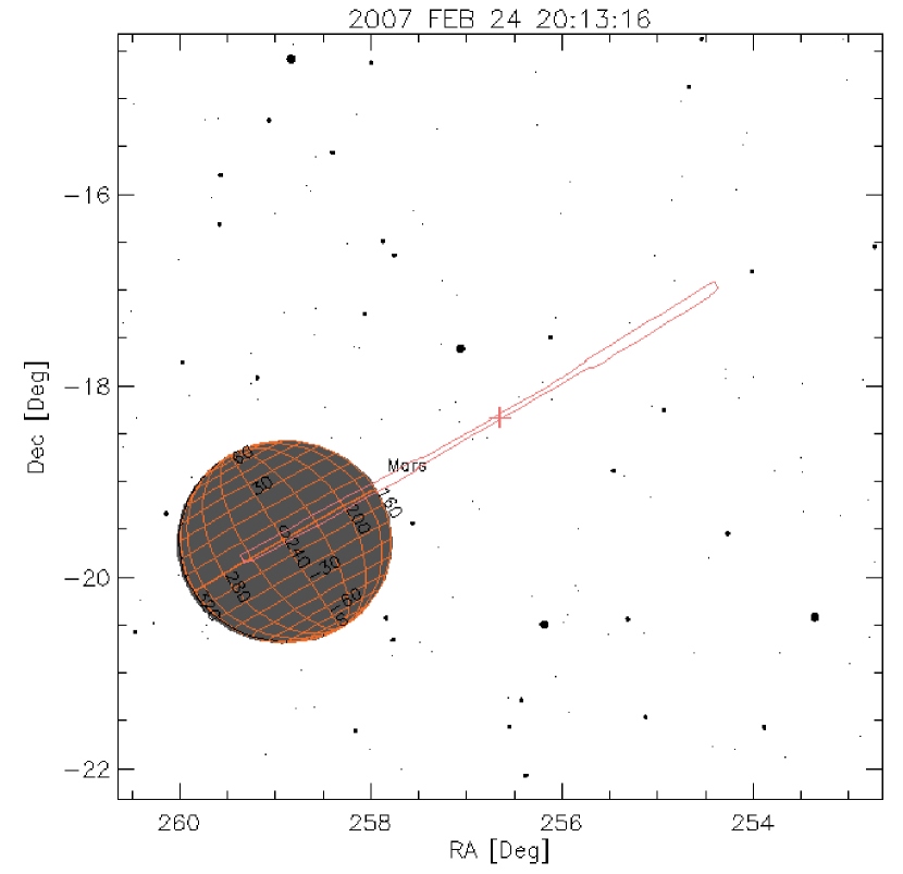
The Alice slit geometry, illustrating the shape of the multi-segment slit, is shown in Fig. 1 for the first pre-CA offset pointing of 2.5∘. The second offset moved the slit an additional 5.0∘ away from Mars parallel to the Martian equator. Except near the limb, the only features seen in the offset spectra are H i Lyman- and Lyman-, and these data are used to extract the spatial profiles of these emissions.
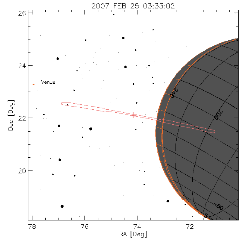
A similar diagram for the post-CA limb scans, beginning 25 February 2007 at UT 03:33:02, is shown in Fig. 2. At this time each spatial pixel projected to 280 km in altitude but as Rosetta receded from Mars the projected size of each pixel increased. The scan slowly shifted the boresight 250 km towards Mars over a 15-minute period. This is illustrated in Fig. 3. Because of the scanning motion, these spectra were acquired in “pixel-list” mode, that is the position of each photon count is recorded together with a time tag so that spectra could be reconstructed with the motion accounted for. Because the Rosetta-Alice instrument has only a single data buffer, the data gaps seen in Fig. 3 result from the time required to read out the buffer to the spacecraft. The typical time to fill the buffer was 30 s, so in practice we accumulated individual spectra corresponding to 30 s integrations. Even so, to detect O i emission at high altitudes, we need to co-add multiple spectra, as described below.
3 Data Analysis
3.1 Calibration
During the gravity assist swing-bys of both Mars and the Earth, the Rosetta instruments were powered on and operated primarily to provide flight verification of instrument performance and to acquire calibration data such as standard ultraviolet star fluxes and detector flat-fields. There were also opportunities to exercise the full range of instrument parameters that could be adjusted by remote command in flight in order to optimize the signal-to-noise performance of the instrument. For the Mars swing-by, the detector high voltage level was set at –3.8 kV. Subsequent operations and analysis showed the optimum setting to be –3.9 kV and all observations beginning in the fall of 2007 were made at that voltage. Nevertheless, by comparison of stellar standards at different voltages (and at different times), we are able to transfer the current absolute flux calibration to the epoch of the Mars swing-by and this is incorporated into the current version of the data pipeline (version 3) with which all of the data have since been processed. The data used in this study are publicly available, both from NASA’s Planetary Data System (http://pdssbn.astro.umd.edu/) and ESA’s Planetary Science Archive (http://www.rssd.esa.int/?project=PSA).
To derive spatial profiles of the observed emissions requires an accurate flat-field calibration. This poses a rather acute problem for Lyman- at 1216 Å because the instrument was designed for this wavelength to fall in the gap between the KBr and CsI photocathode coatings. The intent was to utilize the low detection efficiency of the bare microchannel plate to compensate for the very high expected Lyman- photon flux from the comet. However, because of a slight misalignment in the coating edges, the Lyman- sensitivity varies by a factor of two along the portion of the detector that is mapped onto the sky. In contrast, at Lyman- the variation across the slit is 1.4. There is also a 20% odd-even detector row effect that is accentuated at the lower detector high voltage of –3.8 kV.
Fortuitously, following the Mars encounter, Rosetta-Alice was pointed towards Jupiter and recorded many hours of spectra in support of the New Horizons fly-by of Jupiter in February 2007. These observations were made with the same instrument parameters used for the Mars observations. Since, from the orbit of Mars the Jovian system only filled a single row of the detector, high S/N measurements of detector flat-fields at Lyman- and Lyman- were obtained, together with a measure of grating scattered Lyman- as a function of detector row. An added bonus is that since Jupiter was only 20∘ away on the sky from the coordinates of the offset pointing, these observations provided a measure of the interplanetary Lyman- and Lyman- background for the Mars observations. We used a co-added accumulation of 630,000 s of data obtained between 1 March and 10 March 2007 to derive the flat-fields used in the analysis described below.
3.2 Mars dayglow spectrum
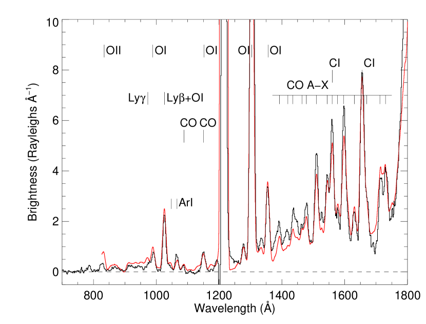
We briefly discuss the dayglow spectrum of Mars, obtained under AL03 pre-CA. It consisted of four exposures, each of 1028 seconds. A composite of the five central rows of the sum of four exposures is shown in Fig. 4. The viewing parameters are given in Table 1. At the start of the sequence, the angular diameter of Mars was 1.62∘ so that the five central rows of the detector were uniformly filled with the illuminated Martian disk. For comparison with previous work, we also show the Mars full disk spectrum recorded by the Hopkins Ultraviolet Telescope (HUT) on board the Space Shuttle in March 1995 (a full solar cycle earlier) (Feldman et al., 2000), convolved to the spectral resolution of Alice. At the time, Mars was 1.666 AU from the Sun, was 70.5∘, and was 75. The HUT spectrum is multiplied by a factor of 0.80 to match the brightness observed by Alice, and this is quite good agreement considering the Alice calibration uncertainty and the fact that the HUT spectrum measured the integrated disk brightness, not just a central stripe of the disk. The comparison also serves to validate the wavelength calibration and provides a reference spectrum with which to compare the exospheric spectra obtained in AL10E and AL11B. As noted by Barth et al. (1972) and Leblanc et al. (2006), with the exception of the H i Lyman series and O i 1304, Mars’ dayglow emissions, principally CO and C i, are confined to altitudes below 200 km.
3.3 Offset exposures
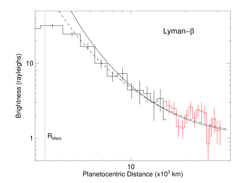
The two offset exposures were taken immediately following the full disk spectra as Rosetta approached Mars. H i Lyman- was detected along the full length of the Alice slit for both offsets. Because the slit is segmented, for each row along the slit the observed Lyman- signal was fit to a gaussian profile superimposed on a grating-scattered background that was fit to a second-order polynomial. The flux was then obtained by integrating under the gaussian and then correcting for the detector flat-field that was derived from subsequent Jupiter observations as described in Section 3.1. The result is shown as a histogram in Fig. 5. The errors shown are statistical in the count rate. The Lyman- profile is similarly derived except that the detector background, due to dark counts, was negligible, and is shown in Fig. 6. The shape of this profile is very similar to the slant intensity profiles derived from the Mariner 6 and 7 fly-bys by Barth et al. (1971), although lower in absolute brightness as the Mariner fly-bys occurred at a time of high solar activity. Neither Fig. 5 nor Fig. 6 have had the interplanetary background subtracted as did the plots of Barth et al. The model fits to the data are discussed below in Section 4.1.
3.4 Limb scan spectra
From the data acquired in pixel list mode during the limb scans schematically illustrated in Fig. 3, we can extract a spectrum spanning a given time interval. However, because the line-of-sight of the spectrogram was changing its position above the limb with time, it is necessary to balance the motion with the need for a sufficiently long integration time to obtain an adequate signal-to-noise ratio for weak emission features. At the same time, we need to avoid contamination of the spectrum by thermospheric emissions. This was done by co-adding the photon counts from the first four exposures for row 14; the first 12 exposures for row 15; and the last 14 exposures for rows 16 and 17. This results in an altitude weighted average with a trapezoidal shape of 320 km centered at 420, 665, 910, and 1240 km, respectively for rows 14 to 17, respectively.
Examples of extracted spectra for rows 15 and 16 are shown in Fig. 7. Note that only H i and O i emissions are detected. A possible feature at 1657 Å in the row 15 spectrum that could be a signature of escaping carbon atoms (Fox and Hać, 1999; Cipriani et al., 2007), is most likely an instrumental artifact as no emission at this wavelength appears in the row 14 spectrum. The background is due to grating scattered Lyman-, which is variable from row to row. Also, the spectra have not been corrected for the odd-even row variation noted in Section 3.1 which is estimated to be 25% for Lyman- and 10% for O i 1304, based on the disk observations discussed in Section 3.2.
4 Discussion
4.1 Exospheric hydrogen model
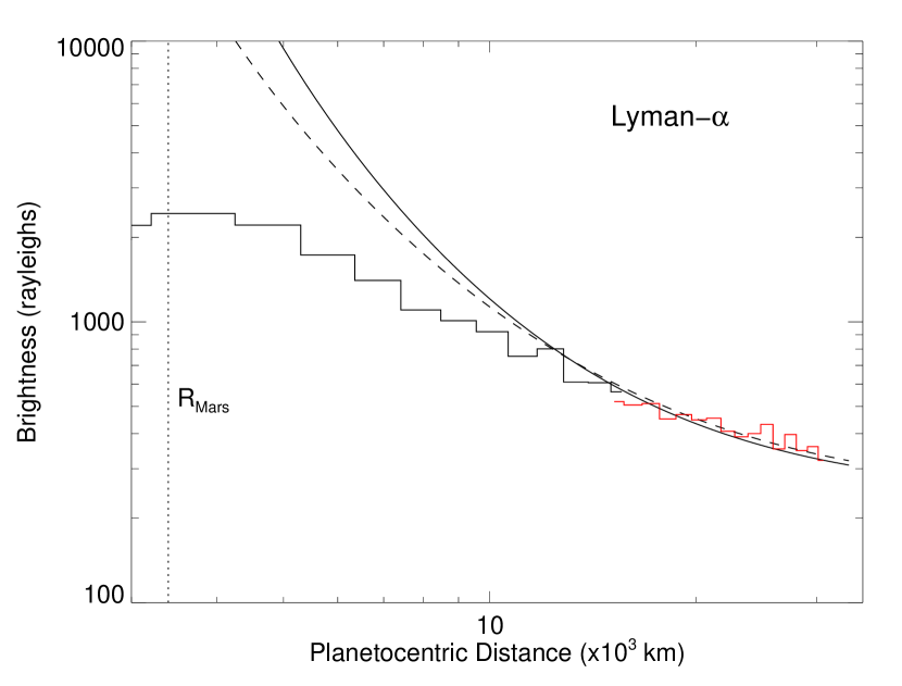
For the analysis of the Lyman- profile we follow the same procedure as Anderson and Hord (1971), using the exospheric model of Chamberlain (1963) but ignoring satellite orbits, as they can be excluded by the observed Lyman- brightness near 30,000 km planetocentric distance. For solar minimum conditions we take the exobase to be at 200 km and the exobase temperature, , to be 200 K (Krasnopolsky, 2002; Fox and Hać, 2009), leaving the hydrogen density at this level as a variable. We assume that Lyman- is optically thin and calculate a fluorescence efficiency (g-factor) of photons s-1 atom-1 at 1 AU using a solar minimum line profile and flux from Lemaire et al. (2002). The interplanetary Lyman- background is fixed at 1.0 rayleigh based on the subsequent Jupiter observations that were used to derive the detector flat-field at 1026 Å (see Section 3.1). All fluxes are referenced to row 15 which is the nominal Alice boresight and which is used for almost all of the stellar calibration measurements.
The result is shown by the solid curve in Fig. 5. The derived H density at 200 km is cm-3 and the escape flux is cm-2 s-1. The model atmosphere is given in Table 2. Optical depth unity along the line-of-sight is at 5,000 km projected planetocentric distance. From the radiative transfer model of Anderson and Hord (1971), applied to the Mariner Lyman- data, we expect the single scattering intensity to be about a factor of two higher than the radiative transfer corrected intensity at this optical depth, and this is consistent with the data shown in Fig. 5. Anderson and Hord, for their solar maximum observations, assuming K at an exobase altitude of 250 km, found an H density and escape flux of cm-3 and cm-2 s-1, respectively. Fig. 5 also shows a model for 260 K (dashed line), which, normalized at 30,000 km, provides what superficially appears to be a better fit to the observed profile. While it is difficult to choose between the models for planetocentric distances greater than 10,000 km, the absence of a strong optical depth effect in the latter suggests that the lower temperature model, corresponding to a typical exospheric temperature at solar minimum, is probably correct. For 260 K, the H density and escape flux are cm-3 and cm-2 s-1, respectively.
The same models, applied to Lyman- using a Lyman-/Lyman- ratio of 250 derived from the IPM measurements, are shown in Fig. 6. The agreement is excellent and the deviation from the optically thin emission is consistent with an optical depth along the line-of-sight of 1 at 10,000 km planetocentric distance. There is no apparent need for a suprathermal H component as suggested by Chaufray et al. (2008) and Clarke et al. (2009).
An interesting measurement of exospheric Lyman- emission from Mars Express has recently been reported by Galli et al. (2006). They found that the Neutral Particle Detector of the ASPERA-3 experiment was sensitive to Lyman- photons and measured a signal, attributed to exospheric hydrogen, out to a tangent height of 7,250 km above the Martian limb. Considering their large measurement uncertainties that include calibration, statistics, pointing, and background subtraction, their measured emission profile is in general accord with the Alice data shown in Fig. 6. However, they interpret this profile in terms of an optically thin resonance scattering model and derive an apparent temperature K. As noted above, we find that the Lyman- emission is optically thick below 10,000 km planetocentric distance (6,600 km above the limb), which leads to a flatter spatial distribution and consequently the appearance of a higher than actual exospheric temperature.
4.2 Two-component oxygen model
For oxygen we use a two-component model, again taking for the cold component, , to be 200 K, and an oxygen density at 200 km of cm-3 (Fox and Hać, 2009). The curve in Fig. 8 represents an added hot component of 1200 K with an oxygen density at 200 km of cm-3 (see Table 2). The density decrease with altitude is considerably faster than the predictions of recent exospheric models of Chaufray et al. (2009) and Valeille et al. (2010) based on a hot atomic O source due to dissociative recombination of O, and which are necessary to support a stoichiometric escape of water vapor from the atmosphere of Mars. However, it has been noted that such inferences from a single viewing geometry during a period of low solar activity can be misleading as this mechanism is quite sensitive to solar activity and is dependent on solar zenith angle at the observation point.
Nevertheless, the present observations raise concern about some of the assumptions and physical parameters used in the recent modeling of oxygen escape from Mars. Fox and Hać (2009), in their comparison of exobase and Monte Carlo models, summarize the literature on modeling efforts from the past few decades and conclude that “efforts to balance the escape rates in the stoichiometric proportion of water are premature.” Fox and Hać focus on a comparison of escape rates and therefore do not compute the oxygen density profiles from their models. Such calculation is warranted by the present data which would allow for a determination of the line-of-sight column densities appropriate to the Alice observations.
Similar questions arise in the analogous modeling of the hot oxygen environment around Venus (Gröller et al., 2010). Bovino et al. (2011) discuss the need for accurate data on energy transfer collisions between hot oxygen atoms and the neutral atmosphere (they are mainly interested in helium) which is at the core of the escape models. Finally, we note that Simon et al. (2009) point out that an additional constraint on the models might be provided by SPICAM measurements of the forbidden O i 2972 (1S – 3P) line, which is produced by both photodissociation of CO2 and by dissociative recombination of O.
5 Conclusion
The Rosetta swing-by of Mars on 25 February 2007, provided the first spectroscopic observations of exospheric hydrogen and oxygen on Mars from outside Mars’ atmosphere since the Mariner 6 and 7 fly-bys in 1969. The spatial distribution of H i Lyman- out to beyond 30,000 km from the planet’s center is similar to that found from Mariner 6 and 7. A Chamberlain model, with current solar minimum model values of exospheric temperature of 200 K and an exobase altitude of 200 km, provides a good fit to the observed Lyman- profile, although the data do not exclude temperatures up to 260 K. A suprathermal component, suggested by several authors, is not needed to match the data. The hydrogen escape flux derived from the 200 K model, cm-2 s-1, is comparable to that derived from the earlier measurements. The distribution of atomic oxygen, derived from 1304 Å emission observed to altitudes of 1000 km above the limb, is not consistent with recent models of oxygen escape based on the production of suprathermal oxygen atoms by dissociative recombination of O.
Acknowledgments
We thank the ESA Rosetta Science Operations Centre (RSOC) and Mission Operations Center (RMOC) teams for their expert and dedicated help in planning and executing the Alice observations of Mars. We thank Darrell Strobel for helpful discussions. The Alice team acknowledges continuing support from NASA’s Jet Propulsion Laboratory through contract 1336850 to the Southwest Research Institute. The work at Johns Hopkins University was supported by a sub-contract from Southwest Research Institute.
References
- Anderson and Hord (1971) Anderson, Jr., D.E., Hord, C.W., 1971. Mariner 6 and 7 ultraviolet spectrometer experiment: Analysis of hydrogen Lyman-alpha data. J. Geophys. Res. 76, 6666–6673.
- Barth et al. (1971) Barth, C.A., Hord, C.W., Pearce, J.B., Kelly, K.K., Anderson, G.P., Stewart, A.I., 1971. Mariner 6 and 7 ultraviolet spectrometer experiment: Upper atmosphere data. J. Geophys. Res. 76, 2213–2227.
- Barth et al. (1972) Barth, C.A., Stewart, A.I., Hord, C.W., Lane, A.L., 1972. Mariner 9 Ultraviolet Spectrometer Experiment: Mars Airglow Spectroscopy and Variations in Lyman Alpha. Icarus 17, 457–468.
- Bovino et al. (2011) Bovino, S., Zhang, P., Gianturco, F.A., Dalgarno, A., Kharchenko, V., 2011. Energy transfer in O collisions with He isotopes and Helium escape from Mars. Geophys. Res. Lett. 38, 2203.
- Chamberlain (1963) Chamberlain, J.W., 1963. Planetary coronae and atmospheric evaporation. Planet. Space Sci. 11, 901–960.
- Chaufray et al. (2008) Chaufray, J.Y., Bertaux, J.L., Leblanc, F., Quémerais, E., 2008. Observation of the hydrogen corona with SPICAM on Mars Express. Icarus 195, 598–613.
- Chaufray et al. (2009) Chaufray, J.Y., Leblanc, F., Quémerais, E., Bertaux, J.L., 2009. Martian oxygen density at the exobase deduced from O I 130.4-nm observations by Spectroscopy for the Investigation of the Characteristics of the Atmosphere of Mars on Mars Express. J. Geophys. Res. 114, 2006.
- Cipriani et al. (2007) Cipriani, F., Leblanc, F., Berthelier, J.J., 2007. Martian corona: Nonthermal sources of hot heavy species. J. Geophys. Res. 112, 7001.
- Clarke et al. (2009) Clarke, J.T., Bertaux, J., Chaufray, J., Gladstone, R., Quemerais, E., Wilson, J.K., 2009. HST Observations Of The Extended Hydrogen Corona Of Mars. Bull. Am. Astron. Soc. 41, 49.11 (abstract).
- Coradini (2010) Coradini, A., et al., 2010. Martian atmosphere as observed by VIRTIS-M on Rosetta spacecraft. J. Geophys. Res. 115, 4004.
- Feldman et al. (2000) Feldman, P.D., Burgh, E.B., Durrance, S.T., Davidsen, A.F., 2000. Far-Ultraviolet Spectroscopy of Venus and Mars at 4 Å Resolution with the Hopkins Ultraviolet Telescope on Astro-2. Astrophys. J. 538, 395–400.
- Fox and Hać (1999) Fox, J.L., Hać, A., 1999. Velocity distributions of C atoms in CO+ dissociative recombination: Implications for photochemical escape of C from Mars. J. Geophys. Res. 104, 24729–24738.
- Fox and Hać (2009) Fox, J.L., Hać, A.B., 2009. Photochemical escape of oxygen from Mars: A comparison of the exobase approximation to a Monte Carlo method. Icarus 204, 527–544.
- Galli et al. (2006) Galli, A., Wurz, P., Lammer, H., Lichtenegger, H.I.M., Lundin, R., Barabash, S., Grigoriev, A., Holmström, M., Gunell, H., 2006. The Hydrogen Exospheric Density Profile Measured with ASPERA-3/NPD. Space Sci. Rev. 126, 447–467.
- Gröller et al. (2010) Gröller, H., Shematovich, V.I., Lichtenegger, H.I.M., Lammer, H., Pfleger, M., Kulikov, Y., Macher, W., Amerstorfer, U.V., Biernat, H.K., 2010. Venus’ atomic hot oxygen environment. J. Geophys. Res. 115, 12017.
- Krasnopolsky (2002) Krasnopolsky, V.A., 2002. Mars’ upper atmosphere and ionosphere at low, medium, and high solar activities: Implications for evolution of water. J. Geophys. Res. 107, 5128.
- Lammer et al. (2003) Lammer, H., Lichtenegger, H.I.M., Kolb, C., Ribas, I., Guinan, E.F., Abart, R., Bauer, S.J., 2003. Loss of water from Mars:Implications for the oxidation of the soil. Icarus 165, 9–25.
- Leblanc et al. (2006) Leblanc, F., Chaufray, J.Y., Lilensten, J., Witasse, O., Bertaux, J., 2006. Martian dayglow as seen by the SPICAM UV spectrograph on Mars Express. J. Geophys. Res. 111, E09S11.
- Lemaire et al. (2002) Lemaire, P., Emerich, C., Vial, J.C., Curdt, W., Schühle, U., Wilhelm, K., 2002. Variation of the full Sun hydrogen Lyman- and profiles with the activity cycle, in: Wilson, A. (Ed.), From Solar Min to Max: Half a Solar Cycle with SOHO, Noordwijk: ESA SP-508. pp. 219–222.
- McElroy (1972) McElroy, M.B., 1972. Mars: An Evolving Atmosphere. Science 175, 443–445.
- Shematovich et al. (2007) Shematovich, V.I., Tsvetkov, G.A., Krestyanikova, M.A., Marov, M.Y., 2007. Stochastic models of hot planetary and satellite coronas: Total water loss in the Martian atmosphere. Solar System Res. 41, 103–108.
- Simon et al. (2009) Simon, C., Witasse, O., Leblanc, F., Gronoff, G., Bertaux, J., 2009. Dayglow on Mars: Kinetic modelling with SPICAM UV limb data. Planet. Space Sci. 57, 1008–1021.
- Stern et al. (2007) Stern, S.A., Slater, D.C., Scherrer, J., Stone, J., Versteeg, M., A’Hearn, M.F., Bertaux, J.L., Feldman, P.D., Festou, M.C., Parker, J.W., Siegmund, O.H.W., 2007. Alice: The Rosetta Ultraviolet Imaging Spectrograph. Space Sci. Rev. 128, 507–527.
- Strickland et al. (1973) Strickland, D.J., Stewart, A.I., Barth, C.A., Hord, C.W., Lane, A.L., 1973. Mariner 9 ultraviolet spectrometer experiment: Mars atomic oxygen 1304-Å emission. J. Geophys. Res. 78, 4547–4559.
- Valeille et al. (2010) Valeille, A., Combi, M.R., Tenishev, V., Bougher, S.W., Nagy, A.F., 2010. A study of suprathermal oxygen atoms in Mars upper thermosphere and exosphere over the range of limiting conditions. Icarus 206, 18–27.
- Valeille et al. (2009) Valeille, A., Tenishev, V., Bougher, S.W., Combi, M.R., Nagy, A.F., 2009. Three-dimensional study of Mars upper thermosphere/ionosphere and hot oxygen corona: 1. General description and results at equinox for solar low conditions. J. Geophys. Res. 114, 11005.
| Observation ID | AL03 | AL10E | AL11B |
|---|---|---|---|
| Start time (UT 2007) | 24 Feb 18:28:14 | 24 Feb 20:13:14 | 25 Feb 03:33:02 |
| Boresight pointing | disk center | offset 2.5∘, 7.5∘ W | E limb scan |
| Distance to Marsa (km) | 239,800 | 184,200 | 51,600 |
| Solar elongationa | 164.3∘ | 164.0∘ | 24.3∘ |
| Longitude of tangent point at limbb | 213.9∘ | 149.7∘ | 263.6∘ |
| Latitude of tangent point at limbb | –1.8∘ | –4.1∘ | –26.5∘ |
| Solar zenith angle at tangent pointb | 15.7∘ | 74.3∘ | 67.9∘ |
| Data mode | Histogram | Histogram | Pixel list |
| Total integration time (s) | 4112 | 483 + 1028 | |
| aAt start of observation. | |||
| bAt sub-observer point for AL03. | |||
| Altitude | H | O (cold) | O (hot) |
|---|---|---|---|
| (km) | (cm-3) | (cm-3) | (cm-3) |
| 200 | 2.50 | 3.00 | 1.00 |
| 400 | 1.69 | 6.86 | 3.70 |
| 600 | 1.19 | 288.0 | 1.49 |
| 800 | 8.61 | 2.04 | 6520. |
| 1000 | 6.42 | 0.023 | 3080. |
| 1200 | 4.90 | 3.7 | 1550. |
| 1400 | 3.82 | 830. | |
| 1600 | 3.03 | ||
| 1800 | 2.44 | ||
| 2000 | 1.99 | ||
| 4000 | 4330. | ||
| 6000 | 1590. | ||
| 8000 | 757. | ||
| 10000 | 422. | ||
| 15000 | 144. | ||
| 20000 | 67.5 | ||
| 25000 | 37.5 | ||
| 30000 | 23.2 | ||
| 35000 | 15.5 |
FIGURE CAPTIONS
Fig. 1. Projection of the Alice slit on the sky with the common boresight offset 2.5∘ from the center of Mars along the equator. Orange grid lines outline the illuminated region of the disk. The shape of the multi-segment slit is shown. Detector row numbers increase from left to right with the boresight (+) in row 15.
Fig. 2. Projection of the Alice slit on Mars at the beginning of the limb scans following closest approach. Orange grid lines outline the illuminated crescent of the disk. Detector row numbers increase from right to left with the boresight (+) in row 15.
Fig. 3. Projection of individual rows of the Alice slit above the Mars limb during the slow limb scan following closest approach. Initially, each spatial pixel projected to 280 km in altitude but as Rosetta receded from Mars the projected size of each pixel increased. The scan also slowly shifted the boresight 250 km towards Mars over a 15-minute period. The cross-hatched areas indicate the time during which photon events were accumulated while the horizontal lines show the times for which photon events were co-added for each row.
Fig. 4. The dayglow spectrum of Mars is a composite of the five central rows of four exposures, each of 1028 seconds. For comparison with previous work, we also show the Mars full disk spectrum recorded by the Hopkins Ultraviolet Telescope (HUT) at 4 Å spectral resolution in March 1995 (a full solar cycle earlier) (Feldman et al., 2000), convolved to the spectral resolution of Alice and multiplied by a factor of 0.8.
Fig. 5. H i Lyman- was detected along the full length of the Alice slit for both offsets. The data are shown as a histogram: black, 2.5∘ offset, red: 7.5∘ offset. The errors shown are statistical in the count rate. Optically thin Chamberlain models without satellite orbits for T=200 K (solid line) and 260 K (dashed line) are shown, superimposed on a 1 rayleigh interplanetary background. The radius of Mars is indicated.
Fig. 6. Same as Fig. 5 for H i Lyman-. The shape of this profile is very similar to the slant intensity profiles derived from the Mariner 6 and 7 fly-bys by Barth et al. (1971), although lower in absolute brightness as the Mariner fly-bys occurred at a time of high solar activity. The same models are shown, superimposed on an interplanetary background of 250 rayleighs.
Fig. 7. Extracted limb scan spectra. For row 15 (top), the photon counts from the first 12 exposures (376 s, see Fig. 3) were co-added. For row 16 (bottom), the last 14 exposures (476 s) were co-added. Only H i and O i emissions are detected.
Fig. 8. Extracted O i 1304 brightness from rows 14–17 as a function of altitude above the Martian limb. The vertical bars illustrate the extent of the trapezoidal altitude weighting function for each row while the horizontal bars are the statistical uncertainty in the count rate. The two-component oxygen model shown is described in the text.