Molecular Photodissociation

4 Molecular photodissociation

4.1 Introduction

Photodissociation is the dominant process by which molecules are removed in any region exposed to intense ultraviolet (UV) radiation. Such clouds of gas and dust are indicated by astronomers with the generic title ‘photon-dominated region’, or PDR. Originally, the term PDR referred mostly to dense molecular clouds close to bright young stars such as found in the Orion nebula. There are many other regions in space, however, in which photodissociation plays a crucial role in the chemistry: this includes diffuse and translucent interstellar clouds, high velocity shocks, the surface layers of protoplanetary disks, and cometary and exoplanetary atmospheres.

In the simplest case, a molecule ABC absorbs a UV photon, which promotes it into an excited electronic state, and subsequently dissociates to AB + C. In reality, the situation is much more complex because there are many electronic states that can be excited, with only a fraction of the absorptions leading to dissociation. Also, there are many possible photodissociation products, each of which can be produced in different electronic, vibrational and rotational states depending on the wavelength of the incident photons. The rate of photodissociation depends not only on the cross sections for all of these processes but also on the intensity and shape of the radiation field at each position in the cloud. Thus, an acccurate determination of the photodissociation rate of even a simple molecule like water involves many detailed considerations, ranging from its electronic structure to its dissociation dynamics and to the specifics of the radiation field to which the molecule is exposed.

In this chapter, each of these steps in determining photodissociation rates is systematically discussed. Section 4.2 reviews the basic processes through which small and large molecules can dissociate following UV absorption. Techniques for determining absorption and photodissociation cross sections through theoretical calculations and laboratory experiments are summarized in Sec. 4.3. This section also mentions new experimental developments that determine branching ratios of the different products. Various interstellar and circumstellar radiation fields are summarized in Sec. 4.4, including their attenuation due to dust and self-shielding deeper inside the cloud. The formulas for computing photodissociation rates are contained in Sec. 4.5, together with references to recent compilations of cross sections and rates. As a detailed example, recent developments in our understanding of the photodissociation of CO and its isotopologs are presented in Sec. 4.6. The chapter ends with a brief review of the photostability of polycyclic aromatic hydrocarbons (PAHs). Much of this chapter follows earlier reviews by [1] and [2].

4.2 Photodissociation processes

4.2.1 Small molecules

The processes by which photodissociation of simple molecules can occur have been outlined by [3] and [4]. A summary is presented in Fig. 4.1 for the case of diatomic molecules. Similar processes can occur for small polyatomic molecules, especially if the potential surface is dissociative along one of the coordinates in the multidimensional space.

The simplest process is direct photodissociation, in which a molecule absorbs a photon into an excited electronic state that is repulsive with respect to the nuclear coordinate. Since spontaneous emission back to the ground state is comparatively slow (typical Einstein-A coefficients of $10^{9}$ s^-1 compared with dissociation times of $10^{13}$ s^-1), virtually all of the absorptions lead to dissociation of the molecule. The resulting photodissociation cross section is continuous as a function of photon energy, and peaks close to the vertical excitation energy according to the Franck-Condon principle. The width is determined by the steepness of the repulsive potential: the steeper the curve, the broader the cross section. Its shape reflects that of the vibrational wavefunction of the ground state out of which the absorption occurs. Note that the cross section is usually very small at the threshold energy corresponding to the dissociation energy $D_{e}$ of the molecule; thus, taking $D_{e}$ as a proxy for the wavelength range at which dissociation occurs gives incorrect results.

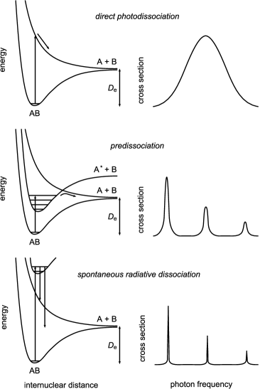
Figure 4.1: Photodissociation processes of diatomic molecules and corresponding cross sections. From top to bottom: direct photodissociation, predissociation and spontaneous radiative dissociation (based on [1]).

In the process of predissociation, the initial absorption occurs into a bound excited electronic state, which subsequently interacts non-radiatively with a nearby repulsive electronic state. An example of such a type of interaction is spin-orbit coupling between states of different spin multiplicity. Another example is the non-adiabatic coupling between two states of the same symmetry. The strength of the interaction depends sensitively on the type of coupling and on the energy levels involved, but predissociation rates are typically comparable to or larger than the rates for spontaneous emission. The effective photodissociation cross section consists in this case of a series of discrete peaks, which reflect the product of the oscillator strength of the initial absorption and the dissociation efficiency of the level involved. The width is controlled by the sum of the radiative and predissociation rates and is generally large ($10^{12}$ s^-1, corresponding to 15 km s^-1 or more in velocity units).

If the excited bound states are not predissociated, spontaneous radiative dissociation can still be effective through emission of photons into the continuum of a lower-lying repulsive state or the vibrational continuum of the ground electronic state. The efficiency of this process is determined by the competition with spontaneous emission into lower-lying bound states. The photodissociation cross section again consists of a series of discrete peaks, but the peaks are not broadened and have widths determined by the total radiative lifetime (typically $<$0.1 km s^-1).

Because a molecule has many excited electronic states that can be populated by the ambient radiation field, in general all of these processes will occur. As an example, Fig. 4.2 shows the potential energy curves of the lowest 16 electronic states of the OH radical: predissociation occurs through the lowest excited $A$ ${}^{2}\Sigma^{+}$ electronic state, whereas direction dissociation can take place through the 1 ${}^{2}\Sigma^{-}$, 1 ${}^{2}\Delta$ and coupled 2 and 3 ${}^{2}\Pi$ electronic states. However, usually only one or two of these processes dominate the photodissociation of a molecule in interstellar clouds. In the case of OH, these are the direct 1 ${}^{2}\Sigma^{-}$ and 1 ${}^{2}\Delta$ channels. However, predissociation through the lower-lying $A$ state is important in cometary atmospheres and disks around cool stars, where the radiation field lacks high-energy photons.

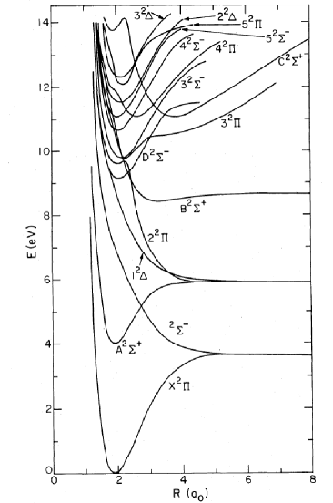
Figure 4.2: Potential energy curves of the OH molecule (reproduced from [5]).

The photodissociation of many simple hydrides like H${}_{2}^{+}$, OH, H₂O, CH, CH⁺, and NH proceeds mostly through the direct process. On the other hand, the photodissociation of CO is controlled by predissociation processes, whereas that of H₂ occurs exclusively by spontaneous radiative dissociation for photon energies below 13.6 eV. Whether the photodissociation is dominated by continuous or line processes has important consequences for the radiative transfer through the cloud (see Sec. 4.4.6).

4.2.2 Large molecules

For large molecules, the same processes as illustrated in Fig. 4.1 can occur, but they become less and less likely as the size of the molecule increases. This is because the number of vibrational degrees of freedom of a non-linear molecule, $3N-6$, increases rapidly with the number of atoms $N$. Each of these modes has many associated vibrational levels, with quantum numbers $v$ increasing up to the dissociation energy of the potential. For sufficiently large $N$, the density of vibrational levels becomes so large that they form a quasi-continuum with which the excited states can couple non-radiatively (Fig. 4.3). Through this so-called process of internal conversion, the molecule ends up in a highly excited vibrational level of a lower-lying electronic state. The probability is small that the molecule will find its way across the multi-dimensional surface to a specific dissociative mode, so the most likely outcome is that the molecule ends up in an excited bound level and subsequently relaxes by emission of infrared photons. Alternatively, the excited molecule can fluoresce down to the ground state in a dipole-allowed electronic transition, or it can undergo so-called intersystem crossing to an electronic state with a different spin multiplicity from which it can phosphoresce down in a spin-forbidden transition.

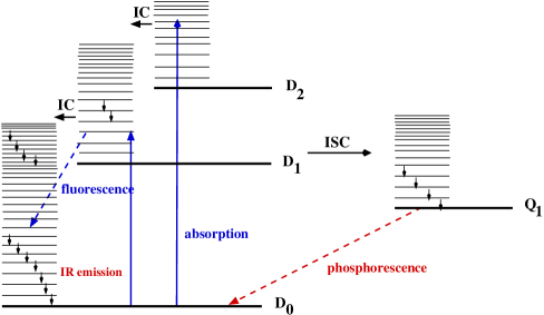
Figure 4.3: Radiative and radiationless decay of large molecules, illustrating the processes of internal conversion (IC), intersystem crossing (ISC), fluorescence, phosphorescence and infrared emission. This example is for a large ion such as PAH⁺ with a ground state with one unpaired electron (doublet spin symmetry) denoted as D₀, and doublet and quartet excited electronic states. Various vibrational levels within the electronic states are indicated.

Statistical arguments using (modified) Rice-Ramsperger-Kassel-Marcus (RRKM) theory suggest that $N$-atom molecules with $N$ ${}_{>}\atop{{}^{\sim}}$25 are stable with respect to photodissociation, although this number depends on the structure and types of modes of the molecule involved [6]. Thus, long carbon chains may have a different photostability than ring molecules. PAHs are a specific class of large molecules highly relevant for astrochemistry, and are discussed further in Sec. 4.7. Very few gas-phase experiments exist on such large molecules to test these theories.

Ashfold et a. [7] have recently pointed out that many intermediate-sized molecules with $N\approx 10$, including complex organic molecules such as alcohols, ethers, phenols, amines and N-containing heterocycles, have dissociative excited states that greatly resemble those found in smaller molecules like H₂O and NH₃. Experiments show that H-loss definitely occurs in these larger systems.

The ionization potentials of large molecules lie typically around 7–8 eV. Most of the absorptions of UV photons with larger energies are expected to lead to ionization but a small fraction can also result in dissociation through highly excited neutral states lying above the ionization threshold or through low-lying dissociative states of the ion itself. These branching ratios are not well determined experimentally.

4.3 Photodissociation cross sections

Quantitative information on photodissociation cross sections comes from theory and experiments. Theory is well suited for small molecules, in particular radicals and ions that are not readily produced in the gas phase. Laboratory measurements of absorption spectra over a wide photon range exist primarily for chemically stable molecules, both small and large. In the following, we first review the theoretical methods of computing potential energy surfaces and cross sections, and then discuss the experimental data.

4.3.1 Theory

All information about a molecule can be contained in a wave function $\Psi$, which is the solution of the time-independent Schrödinger equation

$${\cal H}\Psi({x},{R})=E\Psi({x},{R})$$

Here ${x}$ stands for the spatial and spin coordinates of the $n$ electrons in the molecule and ${R}$ denotes the positions of all $N$ nuclei in the molecule. The total Hamiltonian ${\cal H}$ consists of the sum of the kinetic energy operators of the nuclei $\alpha$ and the electrons and of their potential energies due to mutual interactions. Equation (1) is a $(3n+3N)$-dimensional second order partial differential equation that cannot be readily solved, even for small molecules.

4.3.1.1 Born-Oppenheimer approximation

Because the mass of the nuclei is much larger than that of the electrons, the nuclei move slowly compared with the electrons. Most molecular dynamics studies therefore invoke the Born-Oppenheimer approximation for separating the nuclear and electronic coordinates:

$$\Psi({x},{R})=\Psi^{\rm el}({x};{R})\Psi^{\rm nuc}({x},{R})$$

where the electronic energies $E^{\rm el}({R})$ (also called the potential energy curves or surfaces) are determined by solving the electronic eigenvalue equation with the nuclei held fixed:

$${\cal H}^{\rm el}\Psi^{\rm el}({x};{R})=E^{\rm el}({R})\Psi^{\rm el}({x};{R})$$

Note that $\Psi^{\rm el}$ now only depends parametrically on the nuclear positions $R$. Substituting Equation (2) into (1) and using (3) gives

$$\bigl{[}-\sum_{\alpha}(\frac{1}{2}M_{\alpha})\nabla_{\alpha}^{2}+E^{\rm el}(R)-E\bigr{]}\Psi^{\rm nuc}(R)=0$$

where the sum is over nuclei $\alpha$ with mass $M_{\alpha}$. In this equation, we use the assumption $\nabla_{\alpha}^{2}\Psi^{\rm el}\Psi^{\rm nuc}=\Psi^{\rm el}\nabla_{\alpha}^{2}\Psi^{\rm nuc}$, inherent in the Born-Oppenheimer approximation. Coupling terms involving $\nabla_{\alpha}\Psi^{\rm el}$ are called non-adiabatic terms and their neglect is usually justified. Atomic units (a.u., not to be confused with astronomical units or arbitrary units) have been adopted, which have $\hbar=m_{\rm e}=e=1$. The unit of distance is then 1 a.u. = 0.52918 Å (also called the Bohr radius or $a_{0}$) and the unit of energy is 1 a.u. = 27.21 eV (or Hartree).

Consider for simplicity a diatomic molecule with internuclear distance $R$. The probability of an electronic transition from state $i$ to state $f$ is governed by the magnitude of the electronic transition dipole moment $D(R)$, which can be computed from

$$D(R)=<\Psi^{\rm el}_{f}(r;R)|d|\Psi^{\rm el}_{i}(r;R)>$$

where the integration is performed over the electron coordinate space and $d$ is the electric dipole moment operator in atomic units.

The photodissociation cross section (in cm²) following absorption from a bound vibrational level $v^{\prime\prime}$ of the ground electronic state into the vibrational continuum $k^{\prime}$ of an upper state at a transition energy $\Delta E$ is then given by

$$\sigma_{v^{\prime\prime}}(\Delta E)=2.69\times 10^{-18}g\Delta E|<\Psi^{\rm nuc}_{k^{\prime}}(R)|D(R)|\Psi^{\rm nuc}_{v^{\prime\prime}}(R)>|^{2}$$

where the integration is over the nuclear coordinate $R$. Here $g$ is a degeneracy factor (equal to 2 for $\Pi\leftarrow\Sigma$ transitions, 1 otherwise) and all quantities are in atomic units. Similarly, the absorption oscillator strength between two bound states is

$$f_{v^{\prime}v^{\prime\prime}}={2\over 3}g\Delta E_{v^{\prime}v^{\prime\prime}}|<\Psi^{\rm nuc}_{k^{\prime}}(R)|D(R)|\Psi^{\rm nuc}_{v^{\prime\prime}}(R)>|^{2}$$

Theoretical calculations of photodissociation cross sections thus consist of two steps: (1) calculation of the electronic potential curve or surfaces and (2) solution of the nuclear motion under the influence of the potentials.

4.3.1.2 Electronic energies: method of configuration interaction

Step 1 is the calculation of the electronic potential energy surfaces $E(R)$ and transition dipole moments $D(R)$ connecting the excited states with the ground state as functions of the nuclear coordinate $R$. It is important to realize that most aspects of chemistry deal with small energy differences between large numbers. For example, the binding energy of a molecule or the excitation energy to the first excited state is typically only 0.5% of the total energy of the molecule. Thus, the difficulty in quantum chemistry is not only in dealing with a $3n+3N$ many-body problem, but also in reaching sufficient accuracy in the results. For example, the Hartree-Fock method, in which all electrons are treated as independent particles by expanding the molecular wave function in Equation (2) in a product of $n$ one-electron wave functions, fails because it neglects the ‘correlation energy’ between the electrons: when two electrons come close together, they repel each other. This correlation energy is again on the order of a fraction of a percent of the total energy.

Over the last decades, different quantum chemical techniques have been developed that treat these correlations, and there are several publicly available programs. Most of the standard packages, however, such as the popular GAUSSIAN package, or packages based on density functional theory [8, 9], are only suitable and well-tested for the ground electronic state and for closed-shell electronic structures. More sophisticated techniques based on the CASSCF (complete active space self-consistent field) or coupled cluster methods work well for the lowest few excited electronic states of a molecule, but these states often still lie below the dissociation energy and do not contribute to photodissociation. Accurate calculation of the higher-lying potentials through which photodissociation can proceed requires multi-reference configuration interaction (MR-CI) techniques [10, 11], for which only a few packages exist (e.g., MOLPRO, [12]).

In the CI method, the wave function is expanded into an orthonormal set of $M$ symmetry-restricted configuration state functions (CSFs).

$$\Psi^{\rm el}({x_{1}}...{x_{n}})=\sum_{1}^{M}c_{s}\Phi_{s}({x}_{1}...{x}_{n})$$

The CSFs or ‘configurations’ are generally linear combinations of Slater determinants, each combination having the symmetry and multiplicity of the state under consideration. The Slater determinants are constructed from an orthonormal set of one-electron molecular orbitals (MOs; obtained from an SCF solution to the Hartree-Fock equations), which in turn are expanded in an elementary set of atomic orbitals (AOs; called ‘the basis set’) centered on the atomic nuclei. The larger $M$ is, the more accurate the results.

In the multi-reference technique, a set of configurations is chosen to provide the reference space. For example, the $X$ ${}^{2}\Pi$ ground state of OH has the main configuration $1\sigma^{2}2\sigma^{2}3\sigma^{2}1\pi^{3}$, where $\sigma$ and $\pi$ are the molecular orbitals. The reference space could be chosen to consist of all possible configurations of the same overall symmetry that have a coefficient $c_{s}$ greater than some threshold in the final CI wave function. For the OH example, this includes configurations such as $1\sigma^{2}2\sigma^{2}3\sigma^{1}4\sigma^{1}1\pi^{3}$ in which one electron is excited from the highest occupied MO (HOMO) to the lowest unoccupied MO (LUMO). Alternatively, an ‘active space’ of orbitals can be designated, e.g., the $2\sigma-4\sigma$ and $1\pi-2\pi$ MOs in the case of OH, within which all configurations of a particular symmetry are considered. The CI method then generates all single and double (and sometimes even higher) excitations with respect to this set of reference configurations, several hundreds of thousands of configurations in total, and diagonalizes the corresponding matrix. The resulting eigenvalues are the different electronic states of the molecule, with the lowest energy root corresponding to the ground state.

The quality of an MR-CI calculation is ultimately determined by the choice of the atomic orbital basis set, the choice of the reference space of configurations, and the number of configurations included in the final CI. The basis set needs to be at least of ‘triple-$\zeta$’ quality (i.e., each occupied atomic orbital $1s,2p,...$ is represented by three functions with optimized exponents $\zeta$). Also, polarization and Rydberg functions (i.e., functions which have higher quantum numbers than the occupied orbitals, e.g., $2p$ for H, $3d$ and $4s$ for C) need to be added. The number of AOs chosen in the basis set determines the number of MOs, which in turn determines the number of configurations. For a typical high-quality AO basis set, the latter number is so large, of order $10^{8}$, that some selection of configurations needs to be made in order to handle them with a computer. For example, all configurations which lower the energy by more than a threshold value (in an eigenvalue equation with the reference set) can be chosen to be included in the final CI matrix.

Once the electronic wave functions $\Psi^{\rm el}$ for the ground and excited electronic states have been obtained, the expectation values of other operators, such as the electric dipole moment or the spin-orbit coupling, can be readily calculated.

4.3.1.3 Nuclear dynamics: oscillator strengths and cross sections

Step 2 in calculating photodissociation cross sections consists of solving Eq. (4) to determine the nuclear wave functions using the electronic potential curves from Step 1. Often the nuclear wave function is first separated into a radial and an angular part. If the angular part is treated as a rigid rotor, the radial part can be solved exactly by one-dimensional numerical integration for a diatomic molecule so that no further uncertainties are introduced. Once the wave functions for ground and excited states are obtained, the cross sections can be computed according to Eq. (6).

For indirect photodissociation processes, the oscillator strengths into the discrete upper levels are computed according to Eq. (7) for each vibrational level $v^{\prime}$. If the coupling between the upper bound level with the final dissociative continuum (as computed in Step 1) is weak, first order perturbation theory can be used to calculate the predissociation rates $k^{\rm pr}$ in s^-1. The predissociation probability $\eta_{u}$ of upper level $u$ is then obtained by comparing $k^{\rm pr}$ with the inverse radiative lifetime of the molecule $A^{\rm rad}$: $\eta_{u}=k^{\rm pr}/(k^{\rm pr}+A^{\rm rad})$. In our example of OH, this approximation works well for the calculation of the predissociation of the $A$ ${}^{2}\Sigma^{+}$ state for $v^{\prime}\geq 2$. If the coupling is strong, as is the case for the OH 2 and 3 ${}^{2}\Pi$ states, the coupled equations for the excited states (i.e., going beyond the Born-Oppenheimer approximation) have to be solved in order to compute the cross sections.

For (light) triatomic molecules, the calculation of the full 3D potential surfaces and the subsequent dynamics on those surfaces is still feasible, albeit with significantly more effort involved [13, 4, 14]. For multi-dimensional potential surfaces, often time-dependent wave packet propagation methods are preferred to solve the dynamics rather than the time-independent approach. Besides accurate overall cross sections, such studies give detailed insight into the photodissociation dynamics. For example, the structure seen in the photodissociation of H₂O through the first excited $\tilde{A}$ state is found to be due to the symmetric stretch of the excited molecule just prior to dissociation.

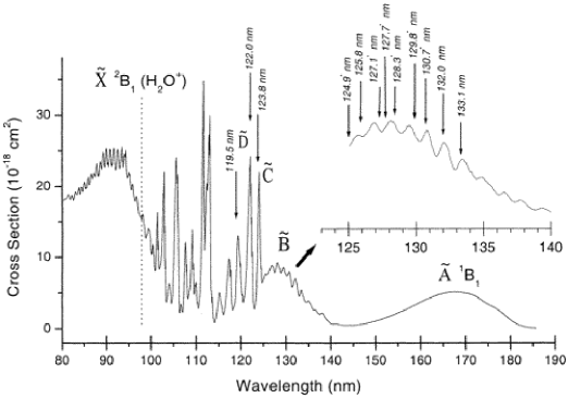
Figure 4.4: Absorption spectrum of gaseous H₂O illustrating the different electronic states through which photodissociation can occur (reproduced from [15]).

For larger polyatomic molecules, such fully flexible calculations are no longer possible and one or more nuclear coordinates need to be frozen. In practice, often the entire nuclear dynamics calculations are skipped and only electronic energies and oscillator strengths at the ground state equilibrium geometry are computed. Assuming that all absorptions into excited states with vertical excitation energies larger than $D_{e}$ lead to dissociation (i.e., $\eta_{u}=1$), this method provides a rough estimate (upper limit) on the dissociation rate [16]. This method works because of the Franck-Condon principle, which states that the highest cross sections occur when the excitation energies are vertical, that is, nuclear coordinates do not change between lower and upper states (Fig. 4.1). Because only a single nuclear geometry has to be considered, the amount of work is orders of magnitude less than that of a full electronic and nuclear calculation.

The overall accuracy of the cross sections and oscillator strengths is typically 20–30% for small molecules in which the number of active electrons is at most $\sim$30. On the order of 5–10 electronic states per molecular symmetry can be computed with reasonable accuracy. Transition energies to the lowest excited states are accurate to $\sim$0.1 eV, those to higher states to 0.2–0.3 eV. Thus, quantum chemistry cannot predict whether a molecule has an electronic state whose excitation energy matches exactly that of, say, Lyman $\alpha$ at 10.2 eV. However, if it has an electronic state with a vertical energy close to 10 eV, and absorption into the state is continuous, theory can firmly state that there is a significant cross section at Lyman $\alpha$. An example is the 1 ${}^{2}\Delta$ state of OH: even with $\pm$30 Å uncertainty in position, the cross section at 1215.6 Å is found to lie between 1 and $2\times 10^{-18}$ cm².

Virtually all molecules have more electronic states below 13.6 eV than can be computed accurately with quantum chemistry. Take our OH example: there is an infinite number of Rydberg states converging to the ionization potential at 13.0 eV. However, because the intensity of the radiation field usually decreases at shorter wavelengths, these higher states do not significantly affect the overall photodissociation rates. Their combined effect can often be taken into account through a single state with an oscillator strength of 0.1 lying around the ionization potential.

4.3.2 Experiments

Laboratory measurements of absorption cross sections have been performed for many chemically stable species, including astrophysically relevant molecules such as H₂O, CO₂, NH₃, and CH₄. Most of these experiments have been performed at rather low spectral resolution, where the individual ro-vibrational lines are not resolved. Figure 4.4 shows an example of measurements for H₂O. A broad absorption continuum is observed between 1900 and 1200 Å, with discrete features superposed at shorter wavelengths. Note that the electronic states responsible for the absorptions at the shortest wavelengths have often not yet been identified spectroscopically.

The absorption of a photon can result in re-emission of another photon, dissociation, or ionization of the molecule, and most experiments do not distinguish between these processes. If the photon energy is below the first ionization potential and if the absorption is continuous, photodissociation is likely to be the dominant process. If not, additional information is needed to infer the dissociation probabilities $\eta_{u}$. For the H₂O example, the broad continuum at 1900–1400 Å corresponds to absorption into the $\tilde{A}$ ${}^{1}B_{1}$ state, which is fully dissociative. However, this is not necessarily true for the higher-lying discrete absorptions. An example is provided by the case of NO for which fluorescence cross sections have been measured directly and found to vary significantly from band to band, with $\eta_{u}$ significantly less than unity for some bands [17].

Experiments typically quote error bars of about 20% in their cross sections if the absorption is continuous. For discrete absorptions, high spectral resolution and low pressures are essential to obtain reliable cross sections or oscillator strengths, since saturation effects can easily cause orders of magnitude errors.

Most broad-band absorption spectra date from the 1950s-1980s and have been summarized in various papers and books [17, 18, 19]. An electronic compilation is provided through the MPI-Mainz UV-VIS spectral atlas. Since about 1990, emphasis has shifted to experiments at single well-defined wavelengths using lasers, in particular at 1930 and 1570 Å. The aim of these experiments is usually to study the dynamics of the photodissociation process at that wavelength, rather than obtaining cross sections. Such studies typically target the lower excited electronic states since lasers or light sources at wavelengths $<$1200 Å are not commonly available except in specialized laboratories [20]. While these sophisticated experiments have provided much basic insight into photodissociation dynamics, the restriction to only one or two wavelengths and lack of cross section data makes them of limited value for interstellar applications.

With the recent advent of powerful synchrotron light sources providing continuous radiation over a large wavelength range, the pendulum is swinging back to more astrophysically relevant results. For example, photodissociation cross sections of molecules such as CH₃OH are being measured in the X-ray regime up to 100 eV [21]. High-resolution data in the FUV regime up to 13.6 eV are eagerly awaited.

4.3.3 Photodissociation products

Inclusion of photodissociation reactions in chemical networks requires knowledge not only of the rate of removal of species ABC, but also of the branching ratios to the various products, AB + C, A + BC or AC + B. Each of these species can be produced with different amounts of electronic, vibrational and/or rotational energy, with the absolute and relative amounts depending on wavelength. None of this detail is captured in the standard tabulations, which, at best, give branching ratios between products integrated over all wavelengths or at a single wavelength, and neglect any vibrational or rotational excitation.

A great number of very elegant modern experiments are now available to explore the fragments, based on a range of photofragment translational spectroscopy and time-resolved photon-electron spectroscopy methods [7]. Product imaging techniques date back to the 1980s and characterize both the velocities, internal energies and angular distributions of the photodissociation products [22].

Velocity map imaging is a recent example of such a technique well suited for probing photodissociation (Fig. 4.5) [23, 24]. In this method, a molecular beam containing the molecule of interest is created by a pulsed supersonic expansion, which ensures internal state cooling. After passing through a skimmer and a small hole in the repeller plate lens of an ion lens assembly the beam is crossed by a dissociation laser beam to form neutral fragments, which are immediately state-selectively ionized by a probe laser beam using resonance enhanced multi-photon ionization (REMPI). The ions retain the velocity information of the nascent photofragments. Velocity map imaging uses a special configuration of an electrostatic immersion ion lens (combination of repeller, extractor, and ground electrodes) to ensure mapping of the ion velocity independent of its position of formation. After acceleration through the ion lens, the particles are mass-selected by time of flight upon reaching the surface of a two-dimensional imaging detector, which converts ion impacts to light flashes recorded by a CCD camera. The two-dimensional image can then be converted to its desired 3-D counterpart by using an inverse Abel transformation. The lens effectively reduces the ‘blurring’ of the images.

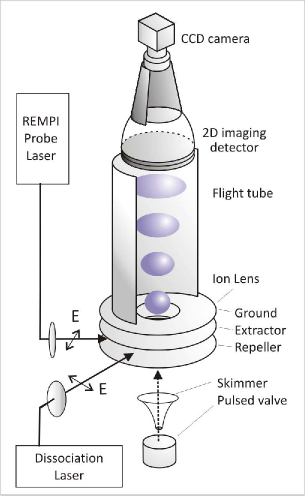
Figure 4.5: Experimental setup for velocity map imaging of photodissociation products (based on [23]).

Another variant on this technique is Rydberg H-atom time of flight spectroscopy. Here the nascent H atoms produced by photodissociation in the ground $n=1$ state are excited into the $n=2$ state using a Lyman $\alpha$ laser at 1216 Å and subsequently to a high Rydberg state with $n=30$–80 using longer wavelength (e.g., 3650 Å) radiation. The neutral Rydberg H atoms then reach a microchannel plate where they are field-ionized and detected.

A completely different set of experiments has been applied to study the branching ratios of large carbon chain molecules. Here, high velocity collisions combined with an inverse kinematics scheme have shown that the most favorable channels are H production from C_nH and C₃ production from C_n [25]. Otherwise the fragmentation behavior is largely statistical.

An example of the complexity of the situation is provided by the OH and H₂O cases. For OH, the potential curves in Fig. 4.2 show that absorption into the 1 ${}^{2}\Sigma^{-}$ state results in ground-state O(³P) + H, but absorption into the higher lying ${}^{2}\Delta$, ${}^{2}\Pi$ and ${}^{2}\Sigma^{+}$ states in excited O(¹D) and O(¹S). The cross sections into these states are such that about equal amounts of O(³P) and O(¹D) are produced in the general interstellar radiation field, but only 5% of O(¹S) [5]. An astrophysical confirmation of this prediction is the detection of the red line of atomic O (¹D $\to$ ³P) at 6300 Å from protoplanetary disks [26, 27]. On the other hand, for radiation fields dominated by lower photon energies such as in comets exposed to solar radiation, the main product is ground-state O(³P).

H₂O is one of the few polyatomic molecules for which the product distribution has been well characterized as a function of energy. Both theory and experiment have shown that absorption at 6–8 eV into the first $\tilde{A}$ electronic state produces OH in the ground electronic ${}^{2}\Pi$ state with some vibrational excitation but little rotational excitation. In contrast, absorption at 9–11 eV into the second $\tilde{B}$ electronic state produces OH in highly excited rotational levels of the $A^{2}\Sigma^{+}$ excited electronic state, but with low vibrational excitation. Absorption into even higher excited states results in O + H₂ or O + H + H products, rather than OH + H. For other polyatomic molecules, experimental information is spotty at best. Early experiments were often performed at high pressures, where the observed products could result from subsequent chemical reactions in the gas that would not occur at the low densities in space [19].

Some guess of the most likely products can be made on the basis of product energies (when does a product channel open up?) and correlation diagrams [7], but these techniques are usually limited to the lowest-lying channels that may not dominate the overall dissociation. Often, the astrochemical databases simply assume a statistical distribution over the various products averaged over all photon energies. Note that the information on the product distribution of species like CH₃OH is relevant not only for gas-phase chemistry but even more so for ice chemistry [28].

4.4 Astrophysical radiation fields

4.4.1 General interstellar radiation field

Determinations of the average intensity of the interstellar radiation field (ISRF) fall into two main categories (see [29] and [30] for critical reviews). The first method is to estimate the number and distribution of hot stars (O, B, A, … type) in the Galaxy, use a model for the dust distribution and properties to determine the absorption and scattering of the stellar radiation, and then sum their fluxes to determine the energy density at a typical interstellar location. This method dates back to [31] and [32], and has most recently been revisited by [33]. The stellar fluxes used in these models are a combination of observed fluxes of early-type stars and extrapolations to shorter wavelengths using model atmospheres.

Figure 4.6: Comparison of the general interstellar radiation field of Draine (1978) (extended for $\lambda>2000$ Å using the representation of [34]) with various stellar radiation fields scaled to have the same integrated intensity from 912–2050 Å. The scaled NEXTGEN model radiation field of a B9.5 star [35] is included as well (dash-dotted). The wavelength ranges where the photodissociation of some important interstellar molecules occurs are indicated (reproduced from [2]).

The second method is to use direct measurements of the UV radiation from the sky at specific wavelengths [36]. Also in this method, model stellar atmospheres are used to provide information at wavelengths not directly observed. In both methods, direct starlight from early B stars is found to dominate the measured interstellar flux. Specifically, most of the flux at a given point in space comes from the sum of discrete sources within 500 pc distance from that point.

The various estimates of the local ISRF in the solar neighborhood agree remarkably well, within a factor of two. The median value found by [33] is within 10% of the mean energy density of $U=8\times 10^{-17}$ erg cm^-3 Å^-1 of [32], averaged over the 912–2070 Å FUV band ($\Delta_{\rm FUV}$). The strength of the one-dimensional interstellar radiation field is often indicated by a scaling factor $G_{0}$ with respect to the flux $F$ in the Habing field ($F_{\rm FUV}=cU_{\rm FUV}\Delta_{\rm FUV}$) of $1.6\times 10^{-3}$ erg cm^-2 s^-1, which is a factor of 1.7 below that of [32]. Thus, the standard Draine field implies $G_{0}=1.7$. Care should be taken that photodissociation rates used in astrochemical models refer to the same radiation field.

If a cloud is located close to a young, hot star, the intensity incident on the cloud boundary may be enhanced by orders of magnitude compared with the average ISRF. A well-known example is the Orion Bar, where the intensity is enhanced by a factor of $4.4\times 10^{4}$ with respect to the Draine field. In contrast, at high latitudes where few early-type stars are located, the intensity may be factors of 5–10 lower in the FUV band than that of the standard ISRF field. Throughout the galactic plane and over time scales of a few Gyr, variations in the local energy density by factors of 2–3 are expected due to the birth and demise of associations containing high-mass O and B stars within about 30 Myr. Moreover, the ratio of the highest-energy photons capable of dissociating H₂ and CO and those in the more general FUV range may vary by a factor of 2 in time and place [33].

4.4.2 Stellar radiation fields

The surface layers of disks around young stars are another example of gas in which the chemistry is controlled by photodissociation. The illuminating stars range from late B- and early A-type stars (the so-called Herbig Ae/Be stars) to K- and M-type stars (the T Tauri stars). For the latter, if the stellar atmosphere dominates the flux, orders of magnitude fewer high-energy photons are available to dissociate the molecules than in the ISRF scaled to the same integrated intensity (Fig. 4.6). In particular, the number of photons capable of dissociating H₂ and CO and ionizing carbon is greatly reduced [2, 37]. However, if accretion onto the star is still taking place, the hot gas in the accreting column produces high-energy photons, including Lyman $\alpha$, which can dominate the FUV flux [38].

4.4.3 Lyman $\alpha$ radiation

Fast shocks (velocities $>$50 km s^-1) produce intense Lyman $\alpha$ radiation due to collisional excitation of atomic hydrogen in the hot gas or recombination of ionized hydrogen [39, 40]. Another prominent line in shocks is the C III resonance line at 977 Å. Fast shocks can be caused by supernovae expanding into the interstellar medium, or by fast jets from protostars interacting with the surrounding cloud. Accretion shocks onto the young star mentioned above are another example, as are exoplanetary atmospheres. Some molecules, in particular H₂, CO and N₂, cannot be dissociated by Lyman $\alpha$. Other simple molecules such as OH, H₂O and HCN can. A recent summary of cross sections at Lyman $\alpha$ is given by [2].

4.4.4 Cosmic-ray induced photons

A dilute flux of UV photons can be maintained deep inside dense clouds through the interaction of cosmic rays with hydrogen in the following process:

$${\rm H\ or\ H_{2}+CR}\to{\rm H^{+}\ or\ H_{2}^{+}+e^{*}}$$

$${\rm e^{*}+H_{2}}\to{\rm H_{2}^{*}+e}$$

$${\rm H_{2}^{*}}\to{\rm H_{2}+h\nu}$$

The energetic electrons e^∗ produced by the cosmic rays excite H₂ into the $B$ ${}^{1}\Sigma_{u}^{+}$ and $C$ ${}^{1}\Pi_{u}$ electronic states, so that the FUV emission is dominated by Lyman- and Werner-band UV photons. Higher-lying electronic states contribute at the shortest wavelengths. As a result, the UV spectrum produced inside dense clouds resembles strongly that of a standard hydrogen lamp in the laboratory. Figure 4.7 shows the UV spectrum computed following [41, 42] for e^∗ at 30 eV and either all H₂ in $J$=0 or distributed over $J$=1 and $J$=0 in a 3:1 ratio. Note that the precise spectrum does depend on the H₂ level populations and the ortho/para ratio. Because of the highly structured FUV field and the lack of high-resolution cross sections for most species, the resulting photodissociation rates may be quite uncertain. On the other hand, the large number of lines has a mitigating effect.

Figure 4.7: Cosmic-ray induced spectrum of H₂ assuming that all H₂ is in $J$=0 (left) or distributed over $J$=1 and $J$=0 in a 3:1 ratio (left). The spectrum shows the number of photons per 1 Å bin for initial 30 eV electrons and are normalized to the total number of ionizations (figure by Gredel, updated from [41, 42]).

4.4.5 Dust attenuation

The depth to which ultraviolet photons can penetrate in the cloud and affect the chemistry depends on (i) the amount of photons at the boundary of the cloud; (ii) the scattering properties of the grains as functions of wavelength; (iii) the competition between the atoms and molecules with the grains for the available photons, which, in turn, depends on the density of the cloud; and (iv) possible self-shielding of the molecules.

The absorption and scattering parameters of the grains determine the penetration depths of photons. The ultraviolet extinction curve shows substantial variations from place to place, especially at the shortest wavelengths in the 912–1100 Å region, which can greatly affect the CO and CN photodissociation rates [43, 44]. Similar variations are expected to occur for the albedo $\varpi$ and the asymmetry parameter $g$ as functions of wavelength, but little is still known about these parameters at the shortest wavelengths [45].

There is considerable observational evidence that dust grains in the surface layers of protoplanetary disks have grown from the typical interstellar size of 0.1 $\mu$m to at least a few $\mu$m in size or more. These large grains extinguish the UV radiation much less, allowing photodissociation to penetrate deeper into the disk [2, 46].

4.4.6 Self-shielding

Because the physical and chemical structure of cloud edges is controlled by the photodissociation of H₂ and CO and photoionization of C, it is important to pay particular attention to the details for these molecules. CO is discussed in Sec. 4.6. The photodissociation of H₂ occurs by absorptions into the Lyman and Werner bands at 912–1100 Å followed by spontaneous emission back to the vibrational continuum of the ground state [47, see also Fig. 4.1]. The absorption lines have typical oscillator strengths $f\approx 0.0001$–0.03, and on average about 10% of the absorptions lead to dissociation. The strongest lines become optically thick at H₂ column densities of $10^{14}$–$10^{15}$ cm^-2 for a Doppler broadening parameter $b$ of 3 km s^-1, implying that molecules lying deeper within the cloud are shielded from dissociating radiation because all relevant photons have been absorbed at the cloud edge (‘self-shielding’). The photodissociation rate of H₂ is about $4.5\times 10^{-11}$ s^-1 in the unattenuated interstellar radiation field, corresponding to a lifetime of about 700 yr. Inside the cloud, the lifetime becomes longer by several orders of magnitude because of the self-shielding process. The remaing 90% of the absorptions are followed by UV fluorescence back into the bound vibrational levels of the H₂ ground state.

Photoionization of atomic carbon has a continuous cross section of about $10^{-17}$ cm² over the 912–1100 Å region. Thus, for column densities $N({\rm C})>10^{17}$ cm^-2, carbon starts to self-shield [48]. Moreover, the saturated absorption bands of H and H₂ over the same wavelength range remove a considerable fraction of the ionizing radiation (‘mutual shielding’).

4.5 Photodissociation rates

The photodissociation rate $k_{pd}$ of a molecule by continuous absorption is given by

$$k_{\rm pd}^{\rm cont}=\int\sigma(\lambda)I(\lambda)d\lambda\ \ {\rm s^{-1}},$$

where $\sigma$ is the cross section for photodissociation in cm² and $I$ is the mean intensity of the radiation in photons cm^-2 s^-1 Å^-1 as a function of wavelength $\lambda$ in Å (Fig. 4.6). For the indirect processes of predissociation and spontaneous radiative dissociation, the rate of dissociation by absorption into a specific level of a bound upper state $u$ from lower level $\ell$ is

$$k_{\rm pd}^{\rm line}={{\pi e^{2}}\over{mc^{2}}}\lambda^{2}_{u\ell}f_{u\ell}\eta_{u}x_{\ell}I(\lambda_{u\ell})\ \ {\rm s^{-1}},$$

where $f_{u\ell}$ is the oscillator strength, $\eta_{u}$ is the dissociation efficiency of the upper level (between 0 and 1), and $x_{\ell}$ is the fractional population in level $\ell$.

The determination of the cross sections and oscillator strengths from theory and experiments has been discussed in Sec. 4.3. Cross section databases are available from [2] at www.strw.leidenuniv.nl/$\sim$ewine/photo and from [49] at amop.space.swri.edu for cometary species. For more complex species also of atmospheric interest, a large compilation is available through the MPI-Mainz UV-VIS spectral atlas at www.atmosphere.mpg.de/enid/2295 and www.science-softcon.de/spectra.

Photodissociation rates as functions of depth into a cloud using the standard interstellar radiation field [32] have been presented for a variety of molecules [1, 45], and most recently by [2]. The latter paper and associated website also summarize rates in cooler radiation fields such as appropriate for late-type stars. The depth dependence due to continuum extinction can be represented by a simple exponential function, with exponents that vary with grain scattering properties and that depend parametrically on cloud thickness. A list of cosmic-ray induced rates for use in dense cloud models has been given by [42].

4.6 Photodissociation of CO and its isotopologs

CO is the most commonly observed molecule in interstellar space and used as a tracer of molecular gas throughout the universe, from local diffuse clouds to dense gas at the highest redshifts. Additional impetus for a good understanding of its photodissociation processes comes from recent interpretations of oxygen isotope fractionation in primitive meteorites, which are thought to originate from isotope selective photodissociation of CO in the upper layers of the disk out of which our solar system formed [50]. To model these processes, information on the electronic structure of all the CO isotopologs, including those with ¹⁷O, is needed.

CO is an extremely stable molecule with a dissociation energy of 11.09 eV, corresponding to a threshold of 1118 Å. It took until the late 1980s to establish that no continuum absorption occurs longward of 912 Å, but that CO photodissociation is dominated by line absorptions, most of which are strongly predissociated [51, 52]. These early laboratory data were used to build a detailed model of the CO photodissociation rate in an interstellar cloud [53, 54]. The depth dependence of the CO photodissociation is affected not only by self-shielding, but also by mutual shielding by H and H₂ because these species absorb in the same wavelength region. ¹²CO, in turn, can shield the less abundant ¹³CO, C¹⁸O and C¹⁷O species, with the amount of shielding depending on the wavelength shifts in the absorption spectrum. Thus, a complete numerical simulation of the entire spectrum of ¹²CO, its isotopologs, H₂ and H is required to correctly compute the attenuation at each depth into a cloud [55, 56].

In the 20 years since these first models, a steady stream of new laboratory data has become available on this key process. In the late 1980s, many of the bands recorded in the laboratory were for ¹²CO only and had no electronic or vibrational designations, so that simulation of the isotopolog spectra involved much guesswork. In particular, the magnitude of the isotopolog shifts depends sensitively on whether $v^{\prime}$ in the upper state is zero or not. Moreover, predissociation rates were generally not known and were simply assumed to be unity. High-resolution spectra for many important bands of ¹²CO, ¹³CO, C¹⁸O and ¹³C¹⁸O were subsequently measured with synchrotron light sources [57, 58, 59, 52]. The fact that the experimental oscillator strengths have now been reconciled with values inferred from astronomical measurements leaves little doubt about their accuracy [60]. Ultra-high-resolution spectra of selected states have been obtained with VUV lasers [20]. These exquisite data provide not only positions down to 0.003 cm^-1 accuracy, but also measure directly the line widths and thus the predissociation probabilities. This is especially important for the $C$ ${}^{1}\Sigma^{+}$ and $E$ ${}^{1}\Pi$ states responsible for most of the isotope-selective effects [61, 62, 63, 64].

Visser et al. [65] used the recent laboratory data to develop a new model for the CO isotope-selective photodissociation including the ¹⁷O isotopologs, and applied it to interstellar clouds and disks around young stars. They also computed shielding functions for a much larger range of CO excitation temperatures and Doppler broadenings. Although the overall rate has changed by only 30%, from $2.0$ to $2.6\times 10^{-10}$ s^-1 for the standard interstellar radiation field [32], the modeled depth dependence differs significantly from earlier work. In particular, the isotope selective effects are diminished by a factor of three or more at temperatures above 100 K. Note, however, that even this new study [65] still had to make many assumptions on line positions, oscillator strengths and predissociation rates for the minor isotopologs, since high-resolution spectra of these minor species have not yet been measured or published. Unexpected differences of up to an order of magnitude have been found between oscillator strengths of ¹²CO and ¹³CO for the same bands, complicating extrapolations from the main isotopologs. These differences likely arise from mixing between various electronic states that depend sensitively on the relative location of the energy levels and may thus differ for a specific ro-vibronic $v^{\prime},J^{\prime}$ level of a particular isotopologue, as found for the case of N₂ [66].

Another set of experiments on the CO isotopolog photodissociation has been carried out using the Berkeley synchrotron source [67] . In contrast with the Paris and Amsterdam results, these data are at comparatively low spectral resolution and were analyzed much more indirectly by following a set of subsequently occurringchemical reactions. The data were interpreted to imply different predissociation probabilities for individual levels of isotopologs caused by near-resonance accidental predissociation processes. In this interpretation, the isotope-selective effects found in meteorites would not require self- or mutual shielding processes. While accidental pre-dissociation is not excluded, these experiments and their conclusions have been challenged on many grounds and are not supported by the higher resolution data cited above [65, 68, 69, 70]. This episode demonstrates that there is no substitute for high-quality molecular physics data in which individual unsaturated lines are recorded, in order to draw astrophysical conclusions.

Another very stable molecule for which the photodissociation occurs primarily by line absorptions is N₂. Thanks to decades of laboratory experiments, the line oscillator strengths and predissociation probabilities of the excited ro-vibrational states are now known with very high accuracy. The N₂ and ¹⁴N¹⁵N data have recently been summarized and applied to interstellar chemistry [71, 72].

Figure 4.8: Photodissociation and photoionization rates of PAHs as functions of number of carbon atoms for the general interstellar radiation field. Solid: loss of C, dotted: loss of H; dash-dotted: ionization. Note the stability of the larger PAHs against dissociation. Figure made using data from [73] following [74].

4.7 Photostability of PAHs

PAH molecules are a class of large molecules that are very stable against photodissociation in the general interstellar medium, explaining their ubiquitous presence in galaxies [75]. However, in clouds exposed to very intense radiation, such as the inner regions of protoplanetary disks and the immediate environments of active galactic nuclei, the smaller PAHs can be destroyed within the lifetime of the source. As discussed in Sec. 4.2.2, the dissociation process of a large molecule involves a multistep process, in which the molecule first absorbs a photon and is promoted to an excited electronic state, then decays non-radiatively to high vibrational levels of the ground state, and finally finds a path to dissociation. The rate of this process thus depends not only on the initial absorption rate, but also on the competition with other processes during these steps. In the first step, the absorption of the photon can also lead to emission of an electron through ionization or photodetachment with probability $\eta_{\rm em}$. In the final step, there is competition between dissociation and cooling by infrared emission. The PAH photodissociation rate thus becomes [76, 74, 77, 78, 73]:

$$k_{\rm pd}=\int(1-\eta_{\rm em})\eta_{\rm diss}\sigma_{\rm abs}I_{\lambda}d\lambda$$

where $\eta_{\rm diss}$ is the yield of a single dissociation process given by

$$\eta_{\rm diss}={\sum_{X}{k_{\rm diss,X}}\over{(k_{\rm diss}+k_{\rm IR})}}.$$

Here $k_{\rm diss,X}$ is the rate for a particular loss channel $X$ (e.g., H removal), $k_{\rm diss}$ is the sum over all such channels, and $k_{\rm IR}$ is the infrared emission rate. Possible loss channels are H, H₂, C, C₂ and C₃ [76], with the rates determined by the RRKM quasi-equilibrium theory according to

$$k_{{\rm diss,}X}=A_{X}{{\rho(E_{\rm int}-E_{0,X})}\over{\rho(E_{\rm int})}}$$

where $A_{X}$ is the pre-exponential Arrhenius factor for channel $X$ and $\rho(E)$ is the density of vibrational states at energy $E$. Dissociation only occurs if the internal energy of the molecule $E_{\rm int}$ exceeds the critical energy $E_{0}$ for a particular loss channel. Values for $E_{0,X}$ were summarized by [73]. The above formulation needs to be modified for clouds exposed to very intense radiation fields ($G_{0}>10^{4}$), when multiphoton events start to become significant, i.e., the PAH molecule absorbs another UV photon before it has cooled down completely. This can significantly increase the dissociation rate.

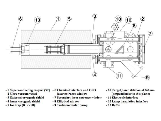
Figure 4.9: Overview of the PIRENEA experiment to study the photostability and fragmentation pattern of PAHs exposed to UV radiation [79].

To compute the dissociation rates, values of $\sigma_{\rm abs}$ as a function of wavelength are essential. The data used in astrophysical models largely come from models developed by [80], based on experiments by [81]. There is also limited experimental information on the loss channels, as summarized by [77]. For example, [82, 83] have measured the photostability of small PAHs of various sizes and shapes against H-loss. Figure 4.8 compares the H-loss channel quantitatively with that of other loss channels and illustrates the competition with ionization.

In a novel experiment, called PIRENEA, the spectroscopy and photodissociation of PAHs into various fragments can be studied [79, 84, 85]. Specifically, gas-phase PAH cations are produced by laser irradiation of a solid target and then guided into an ion cyclotron resonance cell, where they are trapped in a combined magnetic and electric field. The stored ions are irradiated by a xenon lamp (2000–8000 Å) and the products are analyzed by Fourier-transform mass spectrometry. Ions of interest can be selected and isolated by selective ejection of other species. Initial results show that irradiation leads predominantly to atomic hydrogen atom loss, consistent with the work of [82], but loss of C₂H₂ and perhaps even C₄H₂ is also seen from dehydrogenated PAHs [86].

4.8 Summary

This chapter has summarized our understanding of basic photodissociation processes and the theoretical and experimental approaches to determine cross sections, product branching ratios and rates for astrophysically relevant species. The demand for accurate photorates is likely to increase in the coming years as new infrared and submillimeter facilities widen the study of molecules in the surfaces of protoplanetary disks and exoplanetary atmospheres. Critical evaluation of the photodissociation data for these different environments are needed, since rates or cross sections determined for interstellar clouds cannot be simply transposed to other regions.

4.9 Acknowledgments

The authors are grateful to Marc van Hemert and Geert-Jan Kroes for many fruitful collaborations on theoretical studies of photodissociation processes, and to Roland Gredel, Christine Joblin and Dave Parker for providing figures. Support from a Spinoza grant and grant 648.000.002 by the Netherlands Organization of Scientific Research (NWO) and from the Netherlands Research School for Astronomy (NOVA) is gratefully acknowledged.

References

- [1] E. F. van Dishoeck. Photodissociation and photoionization processes, volume 146 of Astrophysics and Space Science Library, pages 49–72. Springer, Berlin, 1988.
- [2] E. F. van Dishoeck, B. Jonkheid, and M. C. van Hemert. Faraday Discussions, 133:231, 2006.
- [3] K. P. Kirby and E. F. Van Dishoeck. Advances in Atomic and Molecular Physics, 25:437–476, 1989.
- [4] R. Schinke. Photodissociation Dynamics. Cambridge University Press, Cambridge, 1993.
- [5] E.F. van Dishoeck and A. Dalgarno. Astrophysical Journal, 277:576, 1984. p. 576.
- [6] P.D. Chowdary and M. Gruebele. Physical Review Letters, 101:250603, 2008. p. 250603.
- [7] M.N.R. Ashfold, G.A. King, and D. et al. Murdock. Phys. Chem. Chem. Phys., 12:1218–38, 2010. p. 1218.
- [8] G. te Velde, F.M. Bickelhaupt, S.J.A. van Gisbergen, et al. Journal of Computational Chemistry, 22:931–967, 2001. p. 931 , www.scm.com.
- [9] Y. Shao, L. F. Molnar, Y. Jung, et al. Phys. Chem. Chem. Phys., 8:3172, 2006. p. 3172.
- [10] R.J. Buenker and S.D. Peyerimhoff. Theor. Chim. Acta, 39:–, 1974. p. 217.
- [11] R.J. Buenker, S.D. Peyerimhoff, and W. Butscher. Molecular Physics, 35:771–791, 1978. p. 771.
- [12] H.-J. et al. Werner. MOLPRO, version 2010.1, 1:0, 2010. www.molpro.net.
- [13] G.J. Kroes, E.F. van Dishoeck, R. Beärda, and M.C. van Hemert. J. Chem. Phys., 99:228–236, 1993. p. 228.
- [14] R.A. Beärda, M.C. van Hemert, and E.F. van Dishoeck. The Journal of Chemical Physics, 102:8930–8941, 1995. p. 8930.
- [15] JH Fillion, R van Harrevelt, J Ruiz, et al. J. Phys. Chem. A, 105(51):11414–11424, 2001.
- [16] M.C. van Hemert and E.F. van Dishoeck. Chem. Phys., 343:292–302, 2008. p. 292.
- [17] L.C. Lee. Astrophys. J., 282:172–177, 1984. p. 172.
- [18] R.D. Hudson. Rev. Geophys. Space Phys., 9:305–406, 1971. p. 305.
- [19] H. Okabe. Photochemistry of Small Molecules. Wiley, New York, 1978.
- [20] W. Ubachs, K.S.E. Eikema, and P.F. Levelt. Astrophys. J., 728:L55–L58, 1994. p. L55.
- [21] S. Pilling, R. Neves, A.C.F. Santos, and H.M. Boechat-Roberty. Astron. Astrophys., 464:393–398, 2007. p. 393.
- [22] D.W. Chandler and P.L. Houston. J. Chem. Phys., 87:1445–1447, 1987. p. 1445.
- [23] Andre T. J. B. Eppink and David H. Parker. Review of Scientific Instruments, 68(9), 1997.
- [24] M. N. R. Ashfold, N. H. Nahler, A. J. Orr-Ewing, et al. Physical Chemistry Chemical Physics (Incorporating Faraday Transactions), 8:26, 2006.
- [25] M. Chabot, T. Tuna, K. Béroff, et al. A&A, 524:A39, 2010.
- [26] H. Storzer and D. Hollenbach. ApJ, 502:L71, 1998.
- [27] B. Acke and M. E. van den Ancker. A&A, 449:267–279, 2006.
- [28] K. I. Öberg, R. T. Garrod, E. F. van Dishoeck, and H. Linnartz. A&A, 504:891–913, 2009.
- [29] J.H. Black. ASP conference series, 58:–, 1994. p. 355.
- [30] E.F. van Dishoeck. ASP Conf. Ser., 59:276, 1994. p. 319.
- [31] H. J. Habing. Bull. Astron. Inst. Netherlands, 19:421, 1968.
- [32] B. T. Draine. ApJS, 36:595–619, 1978.
- [33] A. Parravano, D. J. Hollenbach, and C. F. McKee. ApJ, 584:797–817, 2003.
- [34] E. F. van Dishoeck and J. H. Black. ApJ, 258:533–547, 1982.
- [35] P. H. Hauschildt, F. Allard, J. Ferguson, E. Baron, and D. R. Alexander. ApJ, 525:871–880, 1999.
- [36] R. C. Henry, R. C. Anderson, and W. G. Fastie. Astrophys. J., 239:859–866, 1980.
- [37] I. Kamp and G.-J. van Zadelhoff. A&A, 373:641–656, 2001.
- [38] E. A. Bergin, M. J. Kaufman, G. J. Melnick, R. L. Snell, and J. E. Howe. ApJ, 582:830–845, 2003.
- [39] D. Hollenbach and C. F. McKee. ApJS, 41:555–592, 1979.
- [40] D. A. Neufeld and A. Dalgarno. ApJ, 340:869–893, 1989.
- [41] R. Gredel. Fluorescent and collisional excitation in diatomic molecules. Diss. Naturwiss.-Math. Gesamtfak., Ruprecht-Karls-Univ., Heidelberg, 1987.
- [42] R. Gredel, S. Lepp, A. Dalgarno, and E. Herbst. ApJ, 347:289–293, 1989.
- [43] J. A. Cardelli and B. D. Savage. ApJ, 325:864–879, 1988.
- [44] E. F. van Dishoeck and J. H. Black. ApJ, 340:273–297, 1989.
- [45] W. G. Roberge, D. Jones, S. Lepp, and A. Dalgarno. ApJS, 77:287–297, 1991.
- [46] A. I. Vasyunin, D. S. Wiebe, T. Birnstiel, et al. ApJ, 727:76, 2011.
- [47] A. Dalgarno and T. L. Stephens. ApJ, 160:L107, 1970.
- [48] M. W. Werner. Astrophys. Lett., 6:81, 1970.
- [49] W.F. Huebner, J.J. Keady, and S.P. Lyon. Astrophys. Space Sci., 195, 1992.
- [50] J. R. Lyons and E. D. Young. Nature, 435:317–320, 2005.
- [51] C. Letzelter, M. Eidelsberg, F. Rostas, J. Breton, and B. Thieblemont. Chemical Physics, 114:273–288, 1987.
- [52] G. Stark, K. Yoshino, P. L. Smith, K. Ito, and W. H. Parkinson. ApJ, 369:574–580, 1991.
- [53] Y. P. Viala, C. Letzelter, M. Eidelsberg, and F. Rostas. A&A, 193:265–272, 1988.
- [54] E. F. van Dishoeck and J. H. Black. ApJ, 334:771–802, 1988.
- [55] H.-H. Lee, E. Herbst, G. Pineau des Forets, E. Roueff, and J. Le Bourlot. A&A, 311:690–707, 1996.
- [56] F. Le Petit, C. Nehmé, J. Le Bourlot, and E. Roueff. ApJS, 164:506–529, 2006.
- [57] M. Eidelsberg, J. J. Benayoun, Y. Viala, et al. Astron. Astrophys., 265:839–842, 1992.
- [58] M. Eidelsberg, F. Launay, K. Ito, et al. J. Chem. Phys., 121:292–308, 2004.
- [59] M. Eidelsberg, Y. Sheffer, S. R. Federman, et al. ApJ, 647:1543–1548, 2006.
- [60] Y. Sheffer, S. R. Federman, and B.-G. Andersson. ApJ, 597:L29–L32, 2003.
- [61] P. Cacciani, W. Hogervorst, and W. Ubachs. J. Chem. Phys., 102:8308–8320, 1995.
- [62] P. Cacciani, F. Brandi, I. Velchev, et al. European Physical Journal D, 15:47–56, 2001.
- [63] W. Ubachs, I. Velchev, and P. Cacciani. The Journal of Chemical Physics, 113(2), 2000.
- [64] P. Cacciani and W. Ubachs. Journal of Molecular Spectroscopy, 225:62–65, 2004.
- [65] R. Visser, E. F. van Dishoeck, S. D. Doty, and C. P. Dullemond. A&A, 495:881–897, 2009.
- [66] G. Stark, B. R. Lewis, A. N. Heays, et al. J. Chem. Phys., 128(11):114302, 2008.
- [67] S. Chakraborty, M. Ahmed, T. L. Jackson, and M. H. Thiemens. Science, 321:1328–, 2008.
- [68] S. R. Federman and E. D. Young. Science, 324:1516–, 2009.
- [69] J. R. Lyons, E. A. Bergin, F. J. Ciesla, et al. Geochimica et Cosmochimica Acta, 73:4998–5017, 2009.
- [70] Qing-Zhu Yin, Xiaoyu Shi, Chao Chang, and Cheuk-Yiu Ng. Science, 324(5934):1516, 2009.
- [71] X. Li, A. N. Heays, R. Visser, et al. A&A, 555:A14, 2013.
- [72] A. N. Heays, R. Visser, R. Gredel, et al. A&A, page in press, 2014.
- [73] R. Visser, V. C. Geers, C. P. Dullemond, et al. A&A, 466:229–241, 2007.
- [74] T. Allain, S. Leach, and E. Sedlmayr. A&A, 305:602, 1996.
- [75] A. G. G. M. Tielens. ARA&A, 46:289–337, 2008.
- [76] A. Leger, L. D’Hendecourt, P. Boissel, and F. X. Desert. A&A, 213:351–359, 1989.
- [77] V. Le Page, T. P. Snow, and V. M. Bierbaum. ApJS, 132:233–251, 2001.
- [78] E. Habart, A. Natta, and E. Krügel. A&A, 427:179–192, 2004.
- [79] C. Joblin, C. Pech, M. Armengaud, P. Frabel, and P. Boissel. In M. Giard, J. P. Bernard, A. Klotz, and I. Ristorcelli, editors, EAS Publications Series, volume 4 of EAS Publications Series, pages 73–77, 2002.
- [80] A. Li and B. T. Draine. ApJ, 554:778–802, 2001.
- [81] C. Joblin, A. Leger, and P. Martin. ApJ, 393:L79–L82, 1992.
- [82] H. W. Jochims, E. Ruhl, H. Baumgartel, S. Tobita, and S. Leach. ApJ, 420:307–317, 1994.
- [83] H. W. Jochims, H. Baumgärtel, and S. Leach. ApJ, 512:500–510, 1999.
- [84] C. Joblin and A. G. G. M. Tielens, editors. PAHs and the Universe: A Symposium to Celebrate the 25th Anniversary of the PAH Hypothesis, volume 46 of EAS Publications Series, 2011.
- [85] F. Useli-Bacchitta, A. Bonnamy, G. Mulas, et al. Chemical Physics, 371:16–23, 2010.
- [86] F. Useli Bacchitta and C. Joblin. In Molecules in Space and Laboratory, 2007.