Anomalous diffusion for a correlated process with long jumps

Abstract

We discuss diffusion properties of a dynamical system, which is characterised by long-tail distributions and finite correlations. The particle velocity has the stable Lévy distribution; it is assumed as a jumping process (the kangaroo process) with a variable jumping rate. Both the exponential and the algebraic form of the covariance – defined for the truncated distribution – are considered. It is demonstrated by numerical calculations that the stationary solution of the master equation for the case of power-law correlations decays with time, but a simple modification of the process makes the tails stable. The main result of the paper is a finding that – in contrast to the velocity fluctuations – the position variance may be finite. It rises with time faster than linearly: the diffusion is anomalously enhanced. On the other hand, a process which follows from a superposition of the Ornstein-Uhlenbeck-Lévy processes always leads to position distributions with a divergent variance which means accelerated diffusion.

Keywords: Diffusion; Jumping process; Correlations; Stable Lévy distribution

I Introduction

Stochastic force in the dynamical description of a physical system is usually assumed as a white, Gaussian noise. That approximation may be sufficient if the correlation time is short, compared to the time-scale of the system. However, correlations of the stochastic force are important in many physical problems. Slowly decaying correlations are present in various phenomena including chemical reactions in solutions gro , ligand migration in biomolecules han , atomic diffusion through a periodic lattice iga , spectroscopy fri1 and hydrodynamics tuck ; sane . Long-time memory may also occur in climate, physiology, financial markets and earthquake research lenn ; podo ; podo1 . The paper Ref.rome reported that the normalised prices of both Babylonian and English agricultural commodities exhibited persistent correlations of a power-law type over long periods of up to several centuries. Moreover, long-time correlations emerge in effective, low-dimensional stochastic descriptions of complicated deterministic systems; they are produced by the procedure of fast degrees of freedom removal med ; han1 . Long correlations of the velocity are often connected with the anomalous diffusion: the position variance rises either slower or faster than linearly with time. Examples of anomalous diffusion are frequently encountered in disordered media bou . It has been demonstrated recently that the subdiffusive motion of a polymer is related to scaling of the monomer mean square displacement and the velocity autocorrelation function is algebraic weber . The importance of strong memory (long autocorrelations) – as well as long tails of the distribution– in fluctuations of company profit was stressed in Ref. rom : simple, uncorrelated models are a poor approximation to real market phenomena. Systems with finite correlation time of the stochastic force may be described by the integro-differential Langevin equation. If the memory kernel has the same form as the force autocorrelation function, fluctuation-dissipation relations are satisfied kubo .

Anomalous transport can be described by jumping processes. Continuous time random walk theory (CTRW) met , in particular, predicts subdiffusion which results from the non-Poissonian form of the waiting-time distribution and makes the process non-Markovian. That property is mathematically expressed as a fractional time-derivative in the Fokker-Planck equation. Anomalous diffusion, both super- and subdiffusion, is predicted by a Markovian version of CTRW if one allows for a variable jumping rate kam06 . Besides the waiting-time distribution, CTRW involves the jumping-size distribution. Due to the central limit theorem, stable distributions are distinguished. They can have either the form of a Gaussian or a general stable Lévy distribution, which is characterised by long tails $\sim|x|^{-1-\alpha}$, where $0<\alpha<2$ is the stability index (Lévy flights) shl ; shl1 . Then, the Fokker-Planck equation contains the fractional derivative in respect to the process variable. The above asymptotics implies that variance, as well as all higher moments, must be divergent for any time (the accelerated diffusion). This property means that infinite jumps are performed during a finite time; for that reason Lévy flights are unphysical in dynamical problems. The difficulty can be avoided if one introduces the Lévy walk for which the jump size is strictly related to the time interval met . Those systems can exhibit anomalous diffusion. This is the case for the transport of two-level atoms in optical molasses derived from counterpropagating laser beams mark . The atom which stays for a long time in the potential well may accumulate enough energy, due to spontaneous emissions, to jump above the barrier and perform a long flight. If the depth of the optical potential is small enough, both the momentum autocorrelation function and the position variance obey the power-law dependence; diffusion may be anomalous. One can expect that for the Gaussian processes the system is close to the thermal equilibrium; the detailed balance is then satisfied. It has been recently demonstrated that CTRW with a constant driving force satisfies the Einstein relation for an arbitrary memory kernel kwok .

A jumping process, which is well suited to modelling long-time correlations, is called the ’kangaroo process’ (KP) fri . It is defined by the Poissonian waiting-time distribution with a variable rate. Instead of the jump-size distribution, KP assumes the distribution of the process value just after the jump. As a result, it cannot be described by a differential – either second order or fractional – Fokker-Planck equation, and then it is well suited as a model of non-diffusive processes with strong collisions. KP is a natural formalism to handle the fully developed boundary-layer turbulence since a local description is inadequate in this case dek ; the velocity profile for the Newtonian shear flow is governed by the integro-differential equation of KP. Moreover, a stochastic description of the hyperfine structure of spectral lines is possible by KP since correlations of the radiation emission/absorption operator can be easily taken into account blume1 . For the same reason, KP was applied to describe the stochastic Stark broadening, which involves correlations $\sim 1/t$ fri1 . It can also serve as a model of coloured noises in dynamical problems doe ; plo ; kos .

Considerations involving the correlation problem require some care for the case $\alpha<2$ since the covariance function is infinite. One can introduce a simple modification of the process by cutting the distribution at some large value. Such a truncation procedure is realistic since all physical systems are finite. For example, truncation of the velocity distribution emerges in the natural way in optical molasses since the Doppler force becomes large at high momentum mark . Processes with truncated distributions have finite (co$-$)variance, besides that their properties do not differ from those for the stable distributions tou ; mant .

The aim of this paper is to demonstrate that diffusion – in the presence of the Lévy flights – qualitatively depends on both the correlation form and specific choice of the noise. We consider two models of the particle velocity: a jumping process (KP) and the Ornstein-Uhlenbeck-Lévy (OUL) process. The paper is organized as follows. In Sec.II KP is defined; its properties and stationary solutions are discussed. The distributions of the position and diffusion properties of the system are discussed in Sec.III. In Sec.IV the results are compared with the predictions of a model which is based on the OUL process.

II The jumping process

The process is defined in terms of two probability distributions $Q(\xi)$ and $P_{P}(\tau)$. $Q(\xi)$ determines the step-wise process value just after a jump. More precisely, the probability that one jump occurred in an infinitesimal time interval $(0,\Delta t)$ is given by $\nu(\xi)\Delta t$, where $\nu(\xi)$ denotes a given, variable jumping rate. Therefore, the waiting-time density distribution, $P_{P}(\tau)$, is Poissonian,

$$P_{P}(\tau)=\nu(\xi)\hbox{e}^{-\nu(\xi)\tau};$$ (1)

it determines the probability that the jump occurs for the first time in the interval $(\tau,\tau+\Delta t)$. Immediately after the jump, the probability density of $\xi$ becomes $Q(\xi)$ and the process value remains constant until the next jump. The process is stationary and Markovian, and it can be described by the infinitesimal transition probability $\xi^{\prime}\rightarrow\xi$:

$$p_{tr}(\xi,\Delta t|\xi^{\prime},0)=[1-\nu(\xi^{\prime})\Delta t]\delta(\xi^{\prime}-\xi)+\nu(\xi^{\prime})\Delta tQ(\xi).$$ (2)

Since the time interval $\Delta t$ is small, only one jump is taken into account in the above expression. The first term in Eq.(2) corresponds to the event that no jump occurred. From Eq.(2), the master equation directly follows:

$$\frac{\partial}{\partial t}p(\xi,t)=-\nu(\xi)p(\xi,t)+Q(\xi)\int_{-\infty}^{\infty}\nu(\xi^{\prime})p(\xi^{\prime},t)d\xi^{\prime}.$$ (3)

The stationary solution of Eq.(3) is given by

$$P_{1}(\xi)=\frac{Q(\xi)\langle\nu(\xi)\rangle}{\nu(\xi)}=\frac{Q(\xi)/\nu(\xi)}{\int_{-\infty}^{\infty}Q(\xi^{\prime})/\nu(\xi^{\prime})d\xi^{\prime}},$$ (4)

where the frequency $\nu(\xi)$ is averaged over $P_{1}(\xi)$. Existence of the integral in Eq.(4) imposes appropriate requirements on the functions $Q(\xi)$ and $\nu(\xi)$. However, $P_{1}(\xi)$ is not the only stationary solution of Eq.(3): if $\lim_{\xi\to a}\nu(\xi)/(\xi-a)$ is finite for a constant $a$, a delta function also constitutes a solution. Then, for $a=0$, Eq.(3) implies

$$P_{2}(\xi)=\delta(\xi).$$ (5)

Therefore, the master equation (3) can have the regular solution (Eq.(4)), the singular one (Eq.(5)) or both, according to the specific choice of the functions $Q(\xi)$ and $\nu(\xi)$.

The process is characterised by a broad spectrum of possible covariance functions. We define that quantity in the stationary limit by a joint probability $P$ as

$${\cal C}(\tau)=\langle\xi(t)\xi(t+\tau)\rangle/\langle\xi(t)^{2}\rangle=\int\int\xi\xi^{\prime}P(\xi,t+\tau;\xi^{\prime},t)d\xi d\xi^{\prime}/\langle\xi(t)^{2}\rangle=\int\int\xi\xi^{\prime}P(\xi,t+\tau|\xi^{\prime},t)P_{1}(\xi^{\prime})d\xi d\xi^{\prime}/\langle\xi(t)^{2}\rangle,$$ (6)

where we assume that all the above quantities exist and are finite. ${\cal C}(t)$ can be evaluated by summing up over all possible sequences of jumps kam03 . If both $P_{1}(\xi)$ and $\nu(\xi)$ are even functions, Eq.(6) takes a simple form

$${\cal C}(t)=2\int_{0}^{\infty}\xi^{2}\exp(-\nu(\xi)t)P_{1}(\xi)d\xi/\langle\xi^{2}\rangle.$$ (7)

The integral in Eq.(7) can be expressed in the form $\int_{\nu(0)}^{\infty}\xi^{2}\exp(-\nu(\xi)t)P_{1}(\xi)(d\xi/d\nu)d\nu$ which is essentially a Laplace transform. We want to construct the jumping process for a given covariance by an appriopriate choice of the (even) function $\nu(\xi)$. This can be achieved by inverting the Laplace transform from ${\cal C}(t)$; then $\nu(\xi)$ follows from a simple differential equation

$$\frac{d\nu}{d\xi}=2\xi^{2}P_{1}(\xi)/{\widetilde{{\cal C}}}(\nu),$$ (8)

where ${\widetilde{C}}(\nu)$ denotes the inverse Laplace transform of ${\cal C}(t)$. $\nu(x)$, calculated from Eq.(8), defines the required process as soon as $Q(x)$ is an even function. In particular, for the power-law covariance

$${\cal C}(t)\sim 2\theta\Gamma(\theta)t^{-\theta}~{}~{}~{}~{}~{}~{}~{}~{}~{}(\theta>0),$$ (9)

Eq.(8) yields

$$\nu(\xi)=\left[2\int_{0}^{|\xi|}\xi^{\prime 2}P_{1}(\xi^{\prime})d\xi^{\prime}\right]^{1/\theta}.$$ (10)

In this paper, we assume the stationary distribution $P_{1}(\xi)$ in the form of the stable, symmetric Lévy distribution. It is given by the following Fourier transform

$$P_{1}(\xi)=\frac{1}{\pi}\int_{0}^{\infty}\exp(-Dk^{\alpha})\cos(k\xi)dk,$$ (11)

where the order parameter $\alpha\in(0,2]$. Except for the case $\alpha=2$, which corresponds to the normal distribution, $P_{1}(\xi)$ possesses the algebraic tail $\sim|\xi|^{-\alpha-1}$. Then the variance is divergent and the covariance definition, Eq.(7), does not directly apply. To overcome that difficulty, one introduces modifications to that definition, e.g. the codifference samr ; emb , which can serve as an estimation of the memory loss, or introduces an infinite cascade of Poissonian correlation functions elia . On the other hand, we can approximate the Lévy distribution by introducing a cut-off at some large value of the argument. Those truncated distributions mant ; mant1 ; podo2 ; kop ; sok ; srot are realistic in respect to physical applications, and they agree with the exact ones up to arbitrary large $\xi$ tou ; convergence to the normal distribution is very slow. In the following, ${\cal C}(t)$ will be understood in the sense of the truncated distributions.

In the simplest case of constant jumping rate, $\nu(\xi)=\nu_{0}=$const, the master equation, Eq.(3), takes the form $\frac{\partial}{\partial t}p(\xi,t)=\nu_{0}[Q(\xi)-p(\xi,t)]$. Its solution with the initial condition $p(\xi,0)=\delta(\xi)$,

$$p(\xi,t)=\delta(\xi)\hbox{e}^{-\nu_{0}t}+Q(\xi)(1-\hbox{e}^{-\nu_{0}t}),$$ (12)

converges with time to the unique stationary distribution $P_{1}(\xi)=Q(\xi)$. The exponential form of the covariance follows directly from Eq.(7).

Equality of the distributions $Q(\xi)$ and $P_{1}(\xi)$ does not hold for the variable jumping rate $\nu(\xi)$, cf. Eq.(4). We consider the case of the power-law covariance, Eq.(9). To ensure the existence of $P_{1}(\xi)$, we impose a condition on the parameters $\alpha(\theta+1)>2$; then $\langle\nu(\xi)\rangle<\infty$. On the other hand, the singular solution $P_{2}(\xi)$ (Eq.(5)) also exists if $\theta<3$ because $\nu(\xi)\sim|\xi|^{3/\theta}$ for $|\xi|\ll 1$. Which of those two solutions, $P_{1}(\xi)$ or $P_{2}(\xi)$, is stable? This problem was considered in Ref.sro00 for the constant $P_{1}(\xi)$ on a finite interval. If one approximates the interval length $\tau$ in Eq.(1) by its average, $1/\nu(\xi)$, the process is fully determined by the distribution of $\tau$ ($P(\tau)$) which, in turn, uniquely follows from $P_{1}(\xi)$. However, we are interested in the process value at a given time $t$, i.e. the last interval in the evolution must contain $t$. That requirement imposes a bias, namely longer intervals are more probable. As a result, the effective $P(\tau)$ is modified: it acquires a time dependence and the effective variance dwindles with time to zero. Therefore, the solution $P_{1}(\xi)$ appears unstable, and it decays to the delta function. In the following, we will demonstrate by a numerical analysis that $P_{1}(\xi)$ in the Lévy form is also unstable.

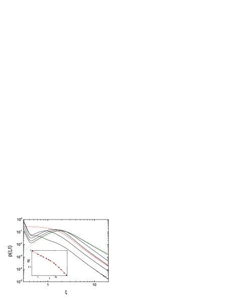
Figure 1: (Colour online) Time evolution of the density distribution $p(\xi,t)$ for algebraic ${\cal C}(t)$. Solid lines correspond to the following times: 0.05, 0.5, 2, 10 and 40 (from top to bottom at large $\xi$). The distribution $P_{1}(\xi)$ is marked by the red dashed line and $Q(\xi)$ by green dots. Inset: relative decay rate of $p(\xi,t)$ (dots) and estimation of that rate by the function $f(t)$, according to Eq.(15) (solid line).

Simulation of the stochastic trajectory requires sampling of the process value $\xi$ from the distribution $Q(\xi)$, which is given by Eq.(4). Details of that procedure – for the Lévy distributed $P_{1}(\xi)$ and the power-law covariance – are presented in Appendix. The procedure is relatively simple if $\theta=1$ and $\alpha=3/2$. In the following, we restrict the numerical simulations to that case. Consecutive time intervals are given by the distribution (1). The time evolution of the density distribution $p(\xi,t)$ is presented in Fig.1, where the initial condition $p(\xi,0)=Q(\xi)$ was assumed. The tail quickly converges to the Lévy shape $|\xi|^{-1-\alpha}$ but its relative strength falls with time. The rate of the decay can be estimated by a function which consists of two power-law segments; it is given by

$$f(t)=\left\{\begin{array}[]{ll}c_{1}t^{-\beta_{1}}&\mbox{for $t\leq 7.5$}\\ c_{2}t^{-\beta_{2}}&\mbox{for $t>7.5$},\end{array}\right.$$ (15)

where $\beta_{1}=0.584$, $\beta_{2}=1.03$, $c_{1}=0.586$ and $c_{2}=1.46$. Decay of the tail is compensated by an increase of the probability density near $\xi=0$: we observe convergence to $P_{2}(\xi)$.

The nonsingular solution becomes stable for large $|\xi|$ after an appropriate variable transformation, $\xi^{\prime}=g(t)\xi$. The function $g(t)$ follows from the requirement that the tail of the new distribution, $P^{\prime}_{1}(\xi^{\prime})\sim|\xi^{\prime}|^{-\alpha-1}$, is time-independent. Using the identity $P^{\prime}_{1}(\xi^{\prime})=P_{1}(\xi)|d\xi/d\xi^{\prime}|$, where $P_{1}(\xi)\sim f(t)|\xi|^{-\alpha-1}$, yields

$$g(t)=\left\{\begin{array}[]{ll}c^{\prime}_{1}t^{\beta^{\prime}_{1}}&\mbox{for $t\leq 7.5$}\\ c^{\prime}_{2}t^{\beta^{\prime}_{2}}&\mbox{for $t>7.5$},\end{array}\right.$$ (18)

where $\beta^{\prime}_{i}=\beta_{i}/\alpha$ and $c^{\prime}_{i}=c_{i}^{-1/\alpha}$. Numerical calculations, presented in Fig.2, confirm that the tail of the limit distribution is stable and coincides with the Lévy one. The decay of the distribution $P_{1}(\xi)$ with time accelerates the decline of the covariance (6): ${\cal C}_{eff}^{(1)}(\tau)=f(\tau){\cal C}(\tau)$. On the other hand, ${\cal C}_{eff}^{(2)}(\tau)=\langle\xi^{\prime}(t)\xi^{\prime}(t+\tau)\rangle/\langle\xi^{\prime}(t)^{2}\rangle=g(\tau){\cal C}(\tau)$. Both covariance functions are presented in Fig.2; they follow the dependence $\tau^{-1-\beta_{1}}$ and $\tau^{-1-\beta_{1}+\beta^{\prime}_{1}}$, respectively.

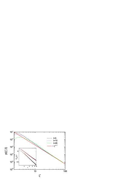
Figure 2: (Colour online) Distribution of KP values as a function of the transformed variable $\xi^{\prime}=g(t)\xi$. Inset: effective autocorrelation functions $C_{eff}^{(i)}(\tau)$, calculated from the definition at $t=1$. The distribution $Q(\xi)$ was truncated at $\xi=10^{4}$. The solid lines have the slopes 1.584 and 1.195.

III Diffusion

Solution of the Fokker-Planck equation for the standard theory of the Brownian motion predicts that the position variance rises linearly with time. Deviations from that pattern may be caused by nonhomogeneity of the medium bou ; kam06 , the presence of regular structures in the phase space gei or memory in the system met . In general, we observe the subdiffusion and superdiffusion (the enhanced diffusion), when the variance rises slower and faster than linearly with time, respectively. Moreover, the accelerated diffusion corresponds to the case of infinite variance for any time. If the process is stationary and the velocity autocorrelation function ${\cal C}(t)$ exists, the time-dependence of the variance is directly related to ${\cal C}(t)$ by a simple identity

$$\langle x^{2}(t)\rangle=2\int_{0}^{t}(t-\tau){\cal C}(\tau)d\tau,$$ (19)

where the average is performed over the stationary distribution. The above formula means that slow decrease of ${\cal C}(t)$ implies fast diffusion. The non-Markovian CTRW with the Gaussian jump-size distribution predicts subdiffusion which results from long waiting times inside the traps. Anomalous diffusion may originate not only from temporal characteristics of the system but also from the spatial structure of the medium. It is the case for transport on fractals hen and for the Markovian CTRW with position-dependent jumping rate kam04 ; all kinds of diffusion are present in those systems kam06 . The stochastic, additive driving force in the Langevin equation with the stable and non-Gaussian distribution leads to the accelerated diffusion. The same conclusion holds for CTRW with the stable jump-size distribution but introducing a power-law truncation may result in heavy tails with convergent variance sok .

We look for the distribution $p_{x}(x,t)$, where the variable $x$ is given by the equation

$$\dot{x}(t)=v(t)$$ (20)

and $v(t)$ follows from the jumping process. In the case $\nu(\xi)=$const, which corresponds to the exponential covariance, we assume $v(t)=\xi(t)$. The distributions $p_{x}(x,t)$ were calculated from individual trajectories $x(t)$; consecutive process values were sampled from the Lévy distribution by a standard procedure wer . Fig.3 presents the results as a function of the Lévy parameter $\alpha$. The tails of all distributions for $\alpha<2$ have the shape $|x|^{-\alpha-1}$ which implies infinite variance and accelerated diffusion. The apparent width of $p_{x}(x,t)$ diminishes with $\alpha$ and rises with time.

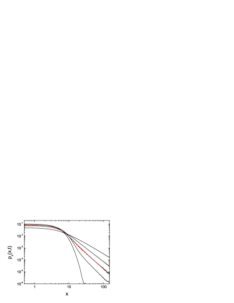
Figure 3: (Colour online) Probability density distributions of the variable $x$ for the case of the exponential covariance at the time $t=5$. The curves correspond to $\alpha=0.8,~{}1.2,~{}1.5,~{}1.8$ and 2 (from right to left); $\nu_{0}=1$. The red dashed line results from inversion of the characteristic function (25) for $\alpha=1.5$ and $\gamma=1/\alpha$.

The case of variable jumping rate involves a coupling between the process values $\xi$ and the waiting times $\tau$, cf. Eq.(10). Since a large $\xi$ corresponds to a small time interval $\tau$, its influence on the particle displacement is limited, and the resulting variance may actually be finite. The condition for the convergence of the variance can be estimated in the following way. We assume $v(t)=\xi(t)$ and take into account only the tail of the Lévy distribution, $\sim\xi^{-\alpha-1}$. Then Eq.(10) yields $\nu(\xi)\sim\xi^{(2-\alpha)/\theta}$. Approximating the time interval by the average of the distribution $P_{P}(\tau)$, $\tau\approx\langle\tau\rangle=1/\nu$, we obtain the trajectory $x(t)$ in the form of a sum of mutually independent variables with the same distribution

$$x(t)=\sum_{i=1}^{n}\xi_{i}^{1+(\alpha-2)/\theta},$$ (21)

where the $n$’th interval contains the time $t$. The distribution of the variable $\eta=\xi_{i}^{1+(\alpha-2)/\theta}$, $P_{\eta}(\eta)$, is given by $P_{\eta}(\eta)=P_{1}[\xi(\eta)]|d\xi/d\eta|\sim\eta^{-1-\alpha\theta/(\alpha+\theta-2)}$. The variance of the distribution $P_{\eta}(\eta)$ is finite if

$$\frac{\alpha\theta}{\alpha+\theta-2}>2.$$ (22)

If the condition (22) is satisfied, the variable $x$ has finite variance as well and its distribution converges with time ($n\to\infty$) to the normal distribution, though that convergence may be very slow. The variance is always finite for the case $\theta=1$, whereas it is always infinite if $\theta\geq 2$. Therefore, a dynamical system in which the velocity is given by KP with the algebraic covariance can be characterised by the finite position variance, although the Lévy stable distribution is assumed. This conclusion is the main result of the paper.

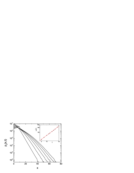
Figure 4: (Colour online) Time evolution of the density distribution $p_{x}(x,t)$ for algebraic ${\cal C}(t)$ and $v(t)=\xi(t)$. The curves correspond to the following times: 5, 10, 15, 20, 25 and 30 (from left to right). Inset: variance as a function of time; the straight line marks the dependence $t^{0.83}$.

The numerical results for the case $v(t)=\xi(t)$, presented in Fig.4, show that the tails of the probability distributions are exponential. The variance rises with time as $t^{0.83}$ up to $t=50$, which dependence indicates subdiffusion. The case of stationary tails, $v(t)=g(t)\xi(t)$, is presented in Fig.5. The results are qualitatively similar to the preceding case but the distributions are broader, and they expand faster with time. The shape of the tails is exponential, $\sim\exp(-\gamma|x|)$, and the parameter $\gamma$ rises with time. The time dependence of the variance is governed by the relation $t^{1.65}$ up to $t=40$, whereas for larger times the growth becomes even faster. Anyway, the dependence is stronger than linear.

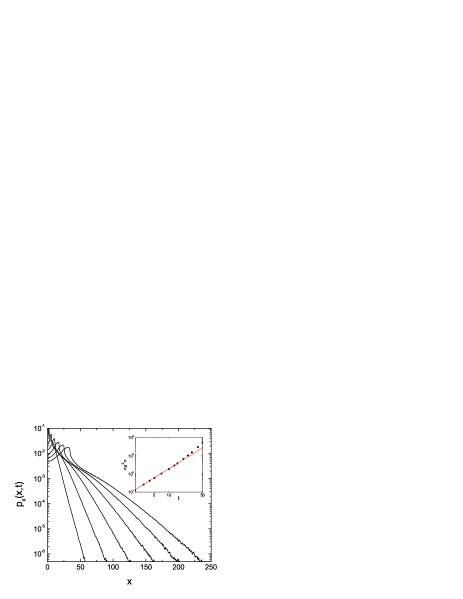
Figure 5: (Colour online) The same as Fig.4 but with $v(t)=g(t)\xi(t)$. The straight line in the inset marks the dependence $t^{1.65}$.

The Langevin equation with uncorrelated noise may predict the finite variance if that noise is multiplicative. That problem was discussed in Ref.sro09 for the algebraic multiplicative factor $|v|^{-\theta/\alpha}$, where $\theta+\alpha>0$. The conclusions depend on a particular interpretation of the stochastic integral. In the Itô interpretation, for which the corresponding Fokker-Planck equation contains a variable diffusion coefficient, the tails of the distribution are the same as for the input noise: $|v|^{-1-\alpha}$. On the other hand, the Stratonovich version predicts the tails $|v|^{-1-\alpha-\theta}$ and the process for the case without potential is subdiffusive if $\alpha+\theta>2$. Heavy tails with finite variance may also emerge when one introduces a deterministic force, both linear and nonlinear sro10 ; che .

IV Comparison with the Ornstein-Uhlenbeck-Lévy process

The Ornstein-Uhlenbeck process describes Brownian particle velocity in the framework of the standard Brownian motion theory gar . The process is defined by the Langevin equation

$$\dot{v}(t)=-\gamma v(t)+\dot{\eta}(t),$$ (23)

where the white noise $\eta(t)$ generates a process with stationary and independent increments. For the Gaussian case, the covariance assumes the exponential form with the decay rate $\gamma$ and (23) is the only process with the above properties, according to the Doob theorem vkam . In the case of the general stable distributions, Eq.(23) defines the Ornstein-Uhlenbeck-Lévy process. Its covariance is also exponential when understood in a sense of truncated distributions sro11 . The probability distribution of the variable $v(t)$ is given by the characteristic function jes

$${\widetilde{p}}(k,t)=\exp\left[-\frac{1}{\alpha\gamma}|k|^{\alpha}(1-{\mbox{e}}^{-\alpha\gamma t})\right];$$ (24)

it converges with time to the stationary distribution. The two-dimensional process $(x,v)$ is Markovian and the probability density $p(x,v,t)$ determines the position distribution after performing integration over velocity sro11 . Its characteristic function reads

$${\widetilde{p}}_{x}(k,t)={\mbox{e}}^{-\sigma(t)|k|^{\alpha}},$$ (25)

where

$$\sigma(t)=\int_{0}^{g}\frac{\kappa^{\alpha}}{1-\kappa}d\kappa$$ (26)

and $g=1-{\mbox{e}}^{-\gamma t}$. According to Eq.(24), OUL process has the same time-scale as KP for $\nu_{0}=\gamma\alpha$, both processes can then be compared. In order to invert the transform (25) we utilise the fact that $p_{x}(x,t)$ is the stable Lévy distribution and it can be expressed as the Fox function sch ; its numerical values follow from series expansions both for small and large $x$. A result of the expansions for $\alpha=1.5$ is compared with the corresponding distribution for KP in Fig.3; both distributions agree.

Processes with long tails of the autocovariance can also be constructed by OUL, namely as their superposition. Following Ref.elia1 , we define a non-Markovian compound process in the form

$$v(t)=\frac{1}{n}\sum_{i=1}^{n}v_{i}(t),$$ (27)

where the atomic parts are OUL processes,

$$\dot{v}_{i}(t)=-\gamma_{i}v_{i}(t)+\dot{\eta}(t),$$ (28)

and $n\to\infty$. The parameter $\gamma$ in the atomic process is a stochastic variable with a given probability distribution $\phi(\gamma)$ which satisfies the normalisation condition $\int_{0}^{\infty}\phi(\gamma)d\gamma=1$. General solution of Eq.(27) and Eq.(28) over the entire real line is given by

$$v(t)=\lim_{n\to\infty}\int_{-\infty}^{t}\frac{1}{n}\sum_{i=1}^{n}{\mbox{e}}^{-\gamma_{i}(t-t^{\prime})}\dot{\eta}(t^{\prime})dt^{\prime}.$$ (29)

Covariance follows from the formula for the atomic process, Eq.(6), where the joint probability distribution has to be conditioned by $\phi(\gamma)$. The final expression involves the Laplace transform:

$${\cal C}(t)=\int_{0}^{\infty}{\mbox{e}}^{-\gamma t}\phi(\gamma)d\gamma.$$ (30)

Eq.(30) can be inverted to obtain $\phi(\gamma)$ for a given form of the covariance. Two examples of the power-law form are presented in Fig.6; ${\cal C}(t)$ was calculated by averaging over an ensemble of trajectories from Eq.(28). The case ${\cal C}(t)=(1-{\mbox{e}}^{-\gamma_{0}t})/(\gamma_{0}t)$ corresponds to $\phi(\gamma)=1/\gamma_{0}$ for $\gamma\leq\gamma_{0}$ and zero elsewhere. The second example involves a slowly decaying tail, $\sim t^{-1/2}$, which appears when we choose $\phi(\gamma)=1/(2\sqrt{\gamma\gamma_{0}})$ ($\gamma\leq\gamma_{0}$). The emergence of long tails in the autocorrelation function results from the presence of small values of $\gamma$ in the integral (30).

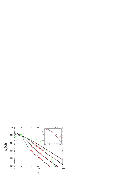
Figure 6: (Colour online) Density distributions $p_{x}(x,t)$ for $v(t)$ which is constructed from the OUL processes according to Eq.(27). The solid lines correspond to $\alpha=1,~{}1.2,~{}1.5$ and 1.8 (from right to left). The solid straight lines mark the dependence $x^{-1-\alpha}$ and the dashed green line the result for $v(t)$ from KP with $\alpha=1.5$. All distributions were calculated at $t=5$. Inset: autocorrelation functions calculated from the trajectory simulations with $\phi(\gamma)=1/\gamma_{0}$ (lower curve) and $\phi(\gamma)=1/(2\sqrt{\gamma\gamma_{0}})$; in both cases $\gamma_{0}=10$. The lower and upper red dashed lines correspond to the functions $(1-{\mbox{e}}^{-\gamma_{0}\tau})/(\gamma_{0}t)$ and $0.15/\sqrt{\tau}$, respectively.

Probability distributions of position, $p_{x}(x,t)$, for $v(t)$ calculated from Eq.(27), are presented in Fig.6. All the curves, which correspond to different values of $\alpha$, assume the power-law shape of the tails, $|x|^{-\alpha-1}$. Therefore, the variance is divergent. Those results are qualitatively different from the distribution for the jumping process which is also presented in the figure.

V Summary and conclusions

We have considered a Markovian jumping process, KP, which is characterised by long jumps and finite correlation time. Its key property is the dependence of the jumping rate on the process value which results, in particular, in a variety of correlation functions. The process value distribution is such that the corresponding master equation has a stationary solution in the form of a Lévy stable distribution with divergent variance. The correlation functions can be properly defined if one introduces a cut-off at some large process value. Numerical analysis, performed for the stability index $\alpha=3/2$ and the power-law correlation function, shows that the stationary solution $P_{1}(\xi)$ is unstable: it decays with time to the delta function. However, the shape of the tails converges with time to that of $P_{1}(\xi)$ and a simple modification of the process – which consists in multiplying the process value by an appropriate function of time – makes the tails stable.

When the particle velocity is assumed as the Lévy distributed jumping process $\xi(t)$, the transport properties of the system are qualitatively dependent on a particular form of its autocorrelation function. The tails of the position distribution for the exponential correlations have the shape $|x|^{-1-\alpha}$, the same as for the velocity, indicating infinite variance. It may not be the case for the power-law form of ${\cal C}(t)$ since long jumps are penalised by small time intervals. It has been demonstrated that if the parameters $\alpha$ and $\theta$ satisfy the condition (22), the position distribution falls relatively fast making the variance finite. Suppressing of long tails of the distribution resembles the Lévy walk approach where the jump length is governed by the time needed to perform the jump. The diffusion process for the case of stable tails appears anomalous; it is characterised by the variance which rises faster than linearly with time. On the other hand, diffusion may be accelerated if condition (22) is not satisfied.

The existence of finite variance of the position distributions – despite long velocity tails – is not a generic property of power-law correlated processes but rather a specific feature of KP. Other processes may exhibit different behaviour; we have demonstrated that a superposition of the OUL processes is characterised by tails of the form $|x|^{-\alpha-1}$ and diffusion is accelerated, similarly to the case of the exponential correlations. Divergence of the variance does not violate physical principles for some problems, e.g. the diffusion on a polymer chain in chemical space or single molecule spectroscopy met . However, in dynamical problems with finite particle mass, a finite propagation velocity is required. From that point of view, KP offers a reasonable alternative to OUL as a model of the noise.

APPENDIX

Random numbers distributed according to $Q(\xi)$ are generated by inversion of the distribution function $\Phi(\xi)$. The following algorithm is restricted to the case $\alpha=1.5$ and $\theta=1$. At first, we numerically evaluate $\nu(\xi)$ from Eq.(10) for consecutive values of $\xi$ up to $\xi_{max}$, with a small step $\Delta\xi$, and store the results. $\xi_{max}$ means the process value for which the Lévy asymptotics is already reached: $P_{1}(\xi)\sim\xi^{-2.5}~{}~{}(\xi>\xi_{max})$. Therefore, we have either $\nu(\xi)=\int_{0}^{\xi}\xi^{\prime 2}P_{1}(\xi^{\prime})d\xi^{\prime}~{}~{}(\xi\leq\xi_{max})$ or $\nu(\xi)=\nu(\xi_{max})+c(\sqrt{\xi}-\sqrt{\xi_{max}})~{}~{}(\xi>\xi_{max})$, where $c$ is a constant. Then we evaluate $\langle\nu(\xi)\rangle$ and $Q(\xi)$ from Eq.(4). We must invert the function $\Phi(\xi)=\int_{0}^{\xi}\nu(\xi^{\prime})P_{1}(\xi^{\prime})d\xi^{\prime}/\langle\nu(\xi)\rangle=r$, where $r\in(0,0.5)$ is a uniformly distributed random number. $\Phi(\xi)$ is calculated numerically and stored if $r\leq\Phi(\xi_{max})$. The asymptotics must be treated separately. Performing the integral yields the equation

$$\Phi(\xi_{max})+c_{1}\xi^{-3/2}+c_{2}\xi^{-1}+c_{3}-r=0,$$ (A1)

which resolves itself to a third-order algebraic equation. Finally, the sign is sampled. In the calculations presented in the paper, the constants have the following values: $\xi_{max}=20$, $c=1.228$, $c_{1}=-2.162$, $c_{2}=-0.725$ and $c_{3}=0.06038$.

The above algorithm may be generalised to other values of $\alpha$ and $\theta$ but in the most cases Eq.(A1) must be solved numerically. Moreover, the integral in the expression for $\Phi(\xi)$ $(\xi>\xi_{max})$ may not be an elementary function if $\theta\neq 1$.

References

- (1) R. F. Grote, J. T. Hynes, J. Chem. Phys. 73 (1980) 2715.
- (2) P. Hänggi, J. Stat. Phys. 30 (1983).
- (3) A. Igarashi, T. Munakata, J. Phys. Soc. Jpn. 57 (1988) 2439.
- (4) A. Brissaud, U. Frisch, J. Quant. Spectrosc. Radiat. Transf. 11 (1971) 1767.
- (5) M. Tuckerman, B.J. Berne, J. Chem. Phys. 98 (1993) 7301.
- (6) J. Sané, J. T. Padding, A. A. Louis, Phys. Rev. E 79 (2009) 051402.
- (7) S. Lennartz, A. Bunde, Phys. Rev. E 79 (2009) 066101.
- (8) B. Podobnik, P. Ch. Ivanov, V. Jazbinsek, Z. Trontelj, H. E. Stanley, I. Grosse, Phys. Rev. E 71 (2005) 025104(R).
- (9) B. Podobnik, H. E. Stanley, Phys. Rev. Lett. 100 (2008) 084102.
- (10) N. E. Romero, Q. D. Y. Ma, L. S. Liebovitch, C. T. Brown, P. Ch. Ivanov, Europhys. Lett. 90 (2010) 18004.
- (11) E. Medina, T. Hwa, M. Kardar, Yi-Cheng Zhang, Phys. Rev. A 39 (1989) 3053.
- (12) P. Hänggi, P. Jung, Adv. Chem. Phys. 89 (1995) 229.
- (13) J.-P. Bouchaud, A. Georges, Phys. Rep. 195 (1990) 127.
- (14) S. C. Weber, J. A. Theriot, A. J. Spakowitz, Phys. Rev. E 82 (2010) 011913.
- (15) H. E. Roman, R. A. Siliprandi, C. Dose, Markus Porto, Phys. Rev. E 80 (2009) 036114.
- (16) R. Kubo, M. Toda, N. Hashitsume, Statistical Physics II (Springer-Verlag, Berlin, 1985).
- (17) R. Metzler, J. Klafter, Phys. Rep. 339 (2000) 1.
- (18) T. Srokowski, A. Kamińska, Phys. Rev. E 74 (2006) 021103.
- (19) M. F. Shlesinger, B. West, Phys. Rev. Lett. 67 (1991) 2106.
- (20) M. F. Shlesinger, Phys. Rev. Lett. 74 (1995) 4959.
- (21) S. Marksteiner, K. Ellinger, P. Zoller, Phys. Rev. A 53 (1996) 3409.
- (22) Kwok Sau Fa, K. G. Wang, Phys. Rev. E 81 (2010) 051126.
- (23) A. Brissaud, U. Frisch, J. Math. Phys. 15 (1974) 524.
- (24) H. Dekker, G. de Leeuw, A. Maassen van den Brink, Phys. Rev. E 52 (1995) 2549.
- (25) M. J. Clauser, M. Blume, Phys. Rev. B 3 (1971) 583.
- (26) C. R. Doering, W. Horsthemke, J. Riordan, Phys. Rev. Lett. 72 (1994) 2984.
- (27) M. Płoszajczak, T. Srokowski, Phys. Rev. E 55 (1997) 5126.
- (28) M. Kostur, J. Łuczka, Acta Phys. Pol. B 30 (1999) 27.
- (29) H. Touchette, E. G. D. Cohen, Phys. Rev. E 80 (2009) 011114.
- (30) R. N. Mantegna, H. E. Stanley, Phys. Rev. Lett. 73 (1994) 2946.
- (31) A. Kamińska, T. Srokowski, Phys. Rev. E 67 (2003) 061114.
- (32) G. Samrodintsky, M.S. Taqqu, Stable Non-Gaussian Random Processes (Chapman & Hall, London, 1994).
- (33) P. Embrechts, M. Maejima, Selfsimilar Processes (Princeton University Press, Princeton, 2002).
- (34) I. Eliazar, J. Klafter, Physica A 376 (2007) 1.
- (35) R. N. Mantegna, H. E. Stanley, Physica A 254 (1998) 77.
- (36) B. Podobnik, P. Ch. Ivanov, Y. Lee, H. E. Stanley, Europhys. Lett. 52 (2000) 491.
- (37) I. Koponen, Phys. Rev. E 52 (1995) 1197.
- (38) I. M. Sokolov, A. V. Chechkin, J. Klafter, Physica A 336 (2004) 245.
- (39) T. Srokowski, Physica A 388 (2009) 1057.
- (40) T. Srokowski, Phys. Rev. Lett. 85 (2000) 2232.
- (41) T. Geisel, A. Zacherl, G. Radons, Phys. Rev. Lett. 59 (1987) 2503.
- (42) H. G. E. Hentschel, I. Procaccia, Phys. Rev. A 29 (1984) 1461.
- (43) A. Kamińska, T. Srokowski, Phys. Rev. E 69 (2004) 062103.
- (44) A. Janicki, A. Weron, Simulation and Chaotic Behavior of -Stable Stochastic Processes (Marcel Dekker, New York, 1994).
- (45) T. Srokowski, Phys. Rev. E 80 (2009) 051113.
- (46) T. Srokowski, Phys. Rev. E 81 (2010) 051110.
- (47) A. Chechkin, V. Gonchar, J. Klafter, R. Metzler, L. Tanatarov, Chem. Phys. 284 (2002) 233.
- (48) C. W. Gardiner, Handbook of Stochastic Methods for Physics, Chemistry and the Natural Sciences (Springer-Verlag, Berlin, 1985).
- (49) N. G. van Kampen, Stochastic Processes in Physics and Chemistry (North-Holland, Amsterdam, 1981).
- (50) T. Srokowski, Acta Phys. Pol. B 42 (2011) 3.
- (51) S. Jespersen, R. Metzler, H. C. Fogedby, Phys. Rev. E 59 (1999) 2736.
- (52) W. R. Schneider, in Stochastic Processes in Classical and Quantum Systems, Lecture Notes in Physics, edited by S. Albeverio, G. Casati, D. Merlini (Springer, Berlin, 1986), Vol. 262.
- (53) I. Eliazar, J. Klafter, Phys. Rev. E 79 (2009) 021115.