CosRayMC: a global fitting method in studying the properties of the new sources of cosmic e± excesses
Abstract
Recently PAMELA collaboration published the cosmic nuclei and electron spectra with high precision, together with the cosmic antiproton data updated, and the Fermi-LAT collaboration also updated the measurement of the total spectrum to lower energies. In this paper we develop a Markov Chain Monte Carlo (MCMC) package CosRayMC, based on the GALPROP cosmic ray propagation model to study the implications of these new data. It is found that if only the background electrons and secondary positrons are considered, the fit is very bad with . Taking into account the extra sources of pulsars or dark matter annihilation we can give much better fit to these data, with the minimum . This means the extra sources are necessary with a very high significance in order to fit the data. However, the data show little difference between pulsar and dark matter scenarios. Both the background and extra source parameters are well constrained with this MCMC method. Including the antiproton data, we further constrain the branching ratio of dark matter annihilation into quarks at confidence level. The possible systematical uncertainties of the present study are discussed.
pacs:
95.35.+d,96.50.S-I Introduction
A very interesting progress made in the recent years in cosmic ray (CR) physics is the discovery of the excesses of positrons and electrons by several space- and ground-based experiments Adriani et al. (2009); Chang et al. (2008); Aharonian et al. (2008, 2009); Abdo et al. (2009). The positron and electron excesses challenge the traditional understanding of CR background. Many theoretical models were proposed to explain these new phenomena, including the astrophysical scenarios (e.g., Yüksel et al. (2009); Hooper et al. (2009a); Delahaye et al. (2009); Shaviv et al. (2009); Hu et al. (2009); Blasi (2009), and see Fan et al. (2010) for a review) and the dark matter (DM) scenario (e.g., Bergström et al. (2008); Barger et al. (2009a); Cirelli et al. (2009); Yin et al. (2009))
Most recently Fermi-LAT team reported the updated measurements of the total spectrum of electrons and positrons, extending to energies as low as several GeV Ackermann et al. (2010). PAMELA collaboration updated the observation of the ratio and the absolute antiproton flux Adriani et al. (2010), and reported the measurement of the pure electron spectrum at the first time Adriani et al. (2011a). The antiproton data extend to GeV, without any hint of deviation from the background contribution Adriani et al. (2010). For the PAMELA electron data, although there is no significant spectral feature above GeV other than a single power-law, it is also consistent with models including extra sources to explain the positron excess Adriani et al. (2011a). There is also hint of hardening of the electron spectrum compared with the low energy part ( GeV), although the solar modulation may be important at these low energies.
Since the accumulation of high-quality CR data, it is now important to extract more information from these data, i.e., estimating the CR background and the possible extra source parameters. Previously, one always constrained one or two parameters with other parameters fixed. This may lead to biased results, especially, when the parameters are strongly correlated. The global fitting procedure searches the maximum likelihood in the multiple dimensional parameter space rather than a reduced one and can give the posterior distribution by marginalizing other parameters in the Bayesian approach. The Markov Chain Monte Carlo (MCMC) procedure, whose computational time scales approximately linearly with the number of parameters, makes it possible to survey in a very large parameter space with the least computational cost.
In our previous studies Liu et al. (2010, 2009), we employed the MCMC method to fit the parameters of the DM scenario as well as the background parameters proposed to explain the excesses. However, the propagation of CRs is treated with a semi-analytical way following Refs. Lavalle et al. (2007, 2008); Maurin et al. (2006). A more precise description of the CR propagation is given by the numerical models, such as GALPROP Strong and Moskalenko (1998) and DRAGON Evoli et al. (2008), in which most of the relevant physical processes are taken into account, and the realistic astrophysical inputs like the interstellar medium (ISM) and the interstellar radiation field (ISRF) are adopted. There are many parameters in the CR propagation model, and it is very difficult to have a full and systematical survey of the parameter space. After embedding the numerical CR propagation tool into the MCMC sampler, we can use it to constrain the model parameters in a more efficient way. Recently there are also several other works using the MCMC method to study the CR propagation Putze et al. (2009, 2010); Trotta et al. (2011).
In this work, we develop a package CosRayMC (Cosmic Ray MCMC), which is comprised of GALPROP, PYTHIA Sjöstrand et al. (2006) and MCMC sampler, to revisit the models to explain the positron and electron excesses and derive the constraints on the model parameters with the latest data. Two kinds of the extra sources are considered: the pulsar scenario and the DM annihilation scenario. In both scenarios we consider the continuous distribution of the sources, although it is possible that one or several nearby pulsars or DM subhalos may explain the excesses Yüksel et al. (2009); Hooper et al. (2009a); Profumo (2008); Hooper et al. (2009b); Kuhlen and Malyshev (2009). As pointed out in Malyshev et al. (2009), it was unlikely that the flux from any single pulsar was significantly larger than that from others given a large number of known nearby and energetic pulsars. For DM subhalos the location and mass are uncertain, which also makes the constraints of the model parameters difficult.
II Propagation of Galactic cosmic rays
The charged particles propagate diffusively in the Galaxy due to the scattering with random magnetic field. There are interactions between the CR particles and the ISM and/or the ISRF, which will lead to fragmentation, catastrophic or continuous energy losses of the particles. For unstable nuclei the radioactive decay also needs to be taken into account. In addition, the overall convection driven by the stellar wind and reacceleration due to the interstellar shock will also affect the distribution function of CRs. For each species of particles we have a partial differential equation to describe the propagation process, with the general form Strong et al. (2007)
| (1) |
where is the density of cosmic ray particles per unit momentum interval, is the source term, is the spatial diffusion coefficient, is the convection velocity, is the diffusion coefficient in momentum space used to describe the reacceleration process, is the momentum loss rate, and are time scales for fragmentation and radioactive decay respectively. Solving the partially coupled equations for all kinds of particles, we can get the propagated results of the CR spectra and spatial distributions. For more details about the terms in Eq. (1) please refer to the recent review paper Strong et al. (2007).
The secondary-to-primary ratios such as B/C and (Sc+Ti+V)/Fe, and the unstable-to-stable ratios of secondary particles such as 10Be/9Be and 26Al/27Al, are often used to constrain the propagation parameters because the ratios can effectively avoid the source parameters. Then one can use the spectra of the primary particles to derive the source parameters. There are some studies to constrain the propagation parameters based on the currently available data (e.g., Maurin et al. (2001); Strong and Moskalenko (1998); Pato et al. (2010a)). In Putze et al. (2009, 2010); Trotta et al. (2011) the MCMC method was adopted to fit both the propagation and source parameters of CRs. However, due to the quality of the observational data, the constraints on the propagation parameters are not very effective, and there may be also large systematic uncertainties.
Since we focus on the electron and positron data in this work, which are not very effective to constrain the propagation parameters, we adopt the best fitting results of the propagation parameters given in Trotta et al. (2011). The main propagation parameters are: cm2s-1, , km s-1, kpc. The injection spectra of nuclei are adopted as (below 10 GV) and (above 10 GV). What we should keep in mind is that there might be systematic errors of the determination of the propagation parameters (see e.g., Maurin et al. (2010)), and the quantitative results of this work might be affected.
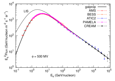
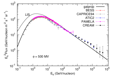
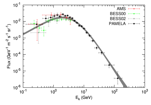
We note that the newest measurements of the CR proton and Helium spectra by CREAM Ahn et al. (2010) and PAMELA Adriani et al. (2011b) showed remarkable deviation of single power-law spectra. Furthermore the spectral indices of proton and Helium are different. Such new features challenge the traditional understanding of the CR origin, acceleration and propagation (see e.g. Ohira and Ioka (2011); Yuan et al. (2011) for some explanations). In the present work we keep the study in the traditional frame and do not try to reproduce the detailed structures of the data. We find that the above adopted injection parameters with proper adjusting of the normalization can basically reproduce the PAMELA-CREAM proton data, as shown in the left panel of Fig. 1. However, when comparing with the Helium data, the model expectation seems to be systematically lower. We increase the relative abundance of Helium in GALPROP by , and give roughly consistent result with PAMELA data (right panel of Fig. 1). The CREAM data can still not be reproduced. Since the contribution to the secondary particles from CR Helium is only a small fraction, we do not think a higher Helium flux within a factor of 2 will substantially affect our following study.
III Methodology
III.1 CosRayMC
The CosRayMC (Cosmic Ray MCMC) code is built up by embedding the CR propagation code GALPROP (GALPROP v51) into the MCMC sampling scheme. The MCMC technique is widely applied to give multi-dimensional parameter constraints from observational data. Following Bayes’ Theorem, the posterior probability of a model (which we refer to a series of parameters ) given the data (which are described by ) is
| (2) |
where is the likelihood function of the model for the data , and is the prior probability of the model parameters. In performing CosRayMC, MCMC is employed to generate a random sample from the posterior distribution which are fair samples of the likelihood surface. Based on the sample, we can get the estimate of the mean values, the variance as well as the confidence level of the model parameters. For details please refer to Lewis and Bridle (2002).
The key improvement, compared with our previous study, is that the calculation of the likelihood are given by calling GALPROP to simulate the mock observations. By doing so, we can have a more precise description of the CR propagation. And as the better data-set is provided in the future, our code can also be used to make a determination of the CR propagation parameters.
For the part with DM contribution to the CRs, the PYTHIA (PYTHIA v6.4) simulation code is employed to calculate the final spectra of electrons, positrons and antiprotons Sjöstrand et al. (2006). Such spectra are then injected into the Galaxy and propagated with GALPROP. The PYTHIA code is also embedded in the CosRayMC code.
III.2 Parameters
We assume the injection spectrum of the background electrons to be a broken power-law function with spectral indices / below/above . Note that for the shock acceleration scenario, the injection spectrum of particles can not be too hard Malkov and O’C Drury (2001). We set the priors that and in the MCMC scanning. The normalization of background electrons , taken as the flux of electrons at GeV, is also regarded as a free parameter. For the background positrons and antiprotons, we adopt the GALPROP model predicted results with the best fitting source and propagation parameters given in Trotta et al. (2011). Considering the fact that there are uncertainties about the ISM density distribution, the hadronic interaction model, and the propagation parameters determined from the secondary-to-primary ratio data, we will further employ factors and to rescale the absolute fluxes of these secondary particle.
For energies below GeV the solar modulation effect is important and needs to be considered. In this work we adopt the force-field approximation to calculate the solar modulation Gleeson and Axford (1968). The modulation potential depends on the solar activity. For the period which PAMELA works the modulation potential is estimated to be MV Adriani et al. (2011b). In our MCMC fit, the modulation potential is also taken as a free parameter. Thus, for the background model we have parameters in total
| (3) |
Pulsars are thought to be the most natural candidates to generate high energy positrons and electrons through the cascade of electrons accelerated in the magnetosphere Zhang and Cheng (2001); Profumo (2008). The spectrum of escaped from the pulsars can be parameterized as power-law with a cutoff at , , where the power-law index ranges from 1 to 2.2 according to the radio and gamma-ray observations Profumo (2008). The cutoff energy of the injected ranges from several tens GeV to higher than TeV, depending on the models and parameters of the pulsars Zhang and Cheng (2001); Malyshev et al. (2009). For the spatial distribution of pulsars, we adopt the following form Lorimer (2004)
| (4) |
where kpc is the distance of solar system from the Galactic center, kpc is the scale height of the pulsar distribution, and . There will be a further normalization factor .
Alternatively, DM annihilation or decay models are widely employed to explain the excesses. Since to date one can not distinguish DM annihilation from decay with the data Liu et al. (2010, 2009), we only consider the annihilation scenario here. Considering the non-excess of PAMELA antiproton data, the DM annihilation final states need to be lepton-dominated Cirelli et al. (2009); Yin et al. (2009). Similar as the previous works Liu et al. (2010, 2009), we do not employ the annihilation final states based on any DM models, but to constrain the final states from the data we use a model-independent way instead. Such constraints will be helpful for the understanding of the DM particle nature.
The annihilation final states are assumed to be two-body , , and 111Since the antiproton productions of various quark flavors do not differ much from each other, here we do not distinguish quark flavors but adopt channel as a typical one of quark final states., with branching ratios , , and respectively. It was also shown that the interactions with low-mass intermediate bosons which then decay to lepton pairs could fit the CR data well Bergström et al. (2009); Cholis et al. (2009). However, since the spectral shapes of the electrons and positrons from these models do not have distinct properties which can be easily distinguished from and , we do not include such final states in this study. The resulting positron, electron and antiproton spectra of these final states are calculated using the PYTHIA simulation package Sjöstrand et al. (2006).
The DM density profile is assumed to be an Einasto type Einasto (1965)
| (5) |
where , kpc and GeV cm-3 according to the recent high resolution simulation Aquarius Navarro et al. (2010). The corresponding local density of DM is about GeV cm-3, which is consistent with the results of a larger local density derived in recent studies Catena and Ullio (2010); Salucci et al. (2010); Pato et al. (2010b). Then the source function of positron produced from DM annihilation is
| (6) |
where is the mass of the DM particle, is the velocity weighted annihilation cross section, is the positron production rate from channel of one annihilation.
The most general parameter space is summerized as below.
| (7) |
For the DM annihilation scenario, we further consider two cases. One is to use the data only in the fit, which can be directly compared with the pulsar scenario. In the other case, the antiproton data are included in order to constrain the coupling to quarks of DM. In the case without the antiproton data, and are set to zero.
IV Results
IV.1 Background
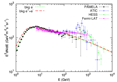
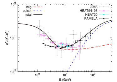
First we run a fit for the pure background contribution. The data included in the fit are PAMELA positron fraction Adriani et al. (2009), PAMELA electron Adriani et al. (2011a), Fermi-LAT total Ackermann et al. (2010), and HESS total Aharonian et al. (2008, 2009).
For the PAMELA positron fraction data, we only employ the data points with GeV in the fit. For the lower energy part we can see that the PAMELA data are inconsistent with the previous measurements. This may be due to more complicated solar modulation effect or even the charge dependent modulation Clem et al. (1996); Beischer et al. (2009); Bobik et al. (2010). It was shown that either a model with different modulation potentials for positive and negative charged particle Beischer et al. (2009) or a detailed Monte Carlo approach to solve the stochastic differential equations of the motion Bobik et al. (2010) can give consistent description to the PAMELA and previous data. The demodulated interstellar spectra of electrons and positrons are also consistent with the conventional CR background model expectation. Here we do not consider the detailed solar modulation models. But note that the solar modulation model may affect the quantitative fitting results. This is one kind of systematical errors.
The best-fit results of the positron fraction and electron (or ) spectra are shown in Fig. 2. The best-fit parameters are compiled in Table 1, with the minimum . Such a large reduced means that the fit is far from acceptable but systematics dominated. Using a goodness-of-fit test we find that the background only case is rejected with a very high significance . That is to say the data strongly favor the existence of additional degrees of freedom. From Fig. 2 we can clearly see that the background model under-estimates both the positron fraction and the total fluxes. The extra sources of are necessary to explain simultaneously the positron fraction and total data.

| bkg | bkg+pulsar | bkg+DM (without ) | bkg+DM (with ) | |
| 1 | ||||
| — | — | — | ||
| 2 | — | — | — | |
| — | — | — | ||
| — | — | — | ||
| — | — | |||
| — | — | |||
| — | — | |||
| — | — | |||
| — | — | |||
| — | — | — | ||
-
1
is in unit of
-
2
is in unit of
The poor fit makes nonsense to discuss the physical implication of the parameters. Therefore we leave the discussion of the parameters in the next subsections, when the extra sources of are taken into account.
IV.2 Pulsar scenario
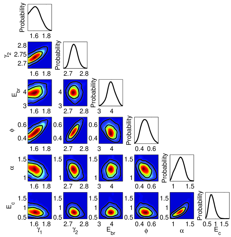

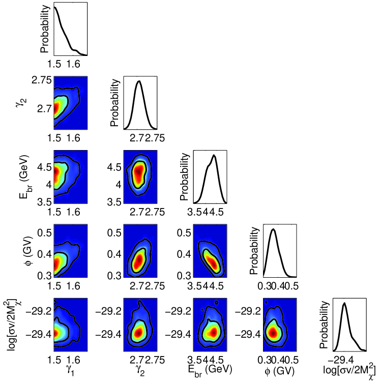
Compared with the conventional GALPROP background model, is consistent with as given in Strong et al. (2004). Note that there is a correlation between parameters and the modulation potential , as shown in Fig. 3. The high energy injection spectrum is softer than as adopted in the conventional model Strong et al. (2004). In the conventional model only the background contribution is employed to fit the data, while here an additional component from the extra sources are added together. Thus the high energy spectrum can be much softer. This might be important for the understanding of the background contribution to the CR electrons.
There is a factor needed for the background positrons to fit the data. As discussed above, such a factor may be ascribed to the uncertainties of the propagation parameters, the ISM density and the strong interaction cross sections. Those uncertainties may be energy-dependent and can not be simply described with a constant factor (see e.g., Delahaye et al. (2009)). For example in this work we use the parameterization given in Kamae et al. (2006) (Kamae06) to calculate the interaction to generate positrons. Compared with the collision model Badhwar77 Badhwar et al. (1977) as adopted in GALPROP, the Kamae06 model gives systematically fewer positrons, especially for energies from several to tens of GeV Delahaye et al. (2009). If these input uncertainties are better understood in the future, we can include the background positron production with a more general form in the MCMC fit.
The fitted parameters for pulsars are , TeV. The constraints of the pulsar parameters are weaker when compared with the background parameters. This is because the cutoff energy is mainly determined by HESS data. However, for HESS data, the very large systematic errors due to poor absolute energy calibration (not shown in Fig. 4) makes it impossible to precisely determine . In the calculation the relative systematic uncertainty of the flux is estimated to be Ackermann et al. (2010). For uncertainty of the energy scale, the flux uncertainty is and for energies below and above TeV. Due to the correlations between and , , the other two parameters are also relatively less constrained.
IV.3 Dark matter annihilation scenario
First we consider the case without including the antiproton data. We found that the background parameters are similar with the pulsar scenario. The overall value of the best-fit is about , which is very close to . That is to say both the astrophysical scenario and DM scenario can give comparable fit to the data. We may not be able to discriminate these two scenarios from the spectra Barger et al. (2009b); Malyshev et al. (2009); Chowdhury et al. (2009); Pohl (2009); Pato et al. (2010c), but need to resort to other probes such as the anisotropy Cernuda (2010) and -rays Zhang et al. (2009).
The fitted mass and cross section of DM are TeV, cm3 s-1. Similar as the pulsar case, these parameters are also less constrained due to the large uncertainties of the HESS data. We can also determine the branching ratios to different flavors of leptons: , and . These results are qualitatively consistent with our previous fit in Liu et al. (2010), but with larger uncertainties because we include the systematic errors of HESS data in the present work. We should be cautious that the determination of the branching ratios may suffer from systematic uncertainties of the background electrons and positrons. As discussed in the previous sub-section, the present understanding of the background positrons is far from precise. Therefore the quoted fitting uncertainties of the branching ratios may be under-estimated.
Then we consider the case with antiproton data. The coupling to quarks of DM annihilation is taken into account. The two dimensional constraints of part of parameters are present in Fig. 5. Compared with the case without antiproton data, we find that the background parameters are slightly different. The reason for the change is mainly due to the low energy spectrum of the background antiprotons. As shown in Fig. 6 the calculated secondary (including tertiary) antiprotons are basically consistent with the PAMELA data for energies higher than several GeV, but under-estimate the flux for the low energy part. This problem was pointed out years ago Moskalenko et al. (2002, 2003), that in the diffusive reacceleration model which gives the best fit to the B/C data the antiprotons are under-estimated. There seems to be a contradiction between the B/C and the antiproton data222Note, however, in Donato et al. (2001) the calculated antiproton flux based on the propagation parameters fitted according to the B/C data Maurin et al. (2001) was consistent with the observational data. As pointed out in Moskalenko et al. (2003) the fit in Maurin et al. (2001) was actually based on the high energy data. And in their results the low energy B/C was in fact over estimated. Furthermore the antiproton production cross sections would also lead to uncertainties Moskalenko et al. (2003). Alternatively, in di Bernardo et al. (2010) a unified model to explain the B/C and antiproton data was proposed, with an empirical modification of the diffusion coefficient at low speed of particles.. To better understand this issue we may need more precise measurement about the B/C data. Back to this work, a lower antiproton flux at low energies will require a smaller solar modulation potential, and therefore the background parameters , and will change accordingly due to the correlations among them as shown in Fig. 5.
One thing important is that we can derive a self-consistent constraint on the quark branching ratio of DM annihilation. The marginalized upper limit of is about . Compared with our previous study Liu et al. (2009) the upper limit of is several times smaller. This is probably due to the bad fit to the antiproton data with the background model. We have run a test to employ the background antiproton spectrum used in Liu et al. (2009) and found that the upper limit of is about , which is consistent with the previous results. This means that the current constraint on is systematics dominated. Better understanding of the background contribution to the antiproton flux is necessary to further address this issue. We plot the range of the antiproton fluxes in Fig. 6.
V Conclusion and Discussion
Recently more and more observational data of CRs with unprecedented precision are available, which makes it possible to better approach the understanding of the basic problems of CRs. Based on MCMC analysis in our previous work Liu et al. (2010, 2009), we embed GALPROP and PYTHIA into MCMC sampler and study the implication of the newest CR data, including the positron fraction, electrons (pure and ) and antiprotons from PAMELA, Fermi-LAT and HESS experiments in this work.
We work in the frame of diffusive reacceleration propagation model of CRs. The propagation parameters are adopted according to the fit to currently available B/C data Trotta et al. (2011), with a slight adjustment of the Helium abundance to better match the PAMELA data Adriani et al. (2011b). We find that the pure background to explain the CR data is disfavored with a very high significance. Therefore it is strongly implied that we may need some extra sources to produce the positrons/electrons.
We then consider two different scenarios, which are widely discussed in recent literature, to explain the excesses. One is the astrophysical scenario with pulsars as the typical example, and the other is the DM annihilation scenario. Using the global fitting method, we can determine the parameters of both the background and the extra sources. The low energy spectral index of the background electrons is consistent with the conventional model adopted in the previous study, while the high energy index is softer in this work. We find that, together with the background contribution, both of these scenarios can give very good fit to the data. For the case with only the data, the goodness-of-fit of the pulsar scenario and DM scenario are almost identical. With the antiproton data included, we can further constrain the coupling to quarks of the DM model. The branching ratio to quarks of the DM annihilation final states is constrained to be at confidence level.
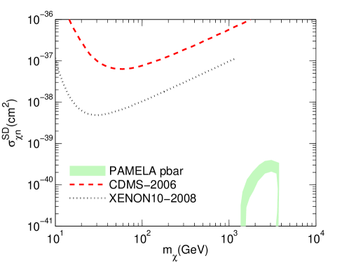
The constraint on the quark branching ratio (or the cross section to quarks) allows us to make a comparison with the direct detection experiments, assuming some effective interaction operators between DM and standard model (SM) particles. As shown in Zheng et al. (2010), generally the constraint of DM-SM coupling from direct experiments is much stronger than the indirect search for spin-independent interactions. However, for the spin-dependent interactions, the indirect search constraint could be comparable or stronger than the direct experiments. In Fig. 7 we give the constraints on the spin-dependent DM-neutron scattering cross section according to the cross section of DM annihilation to quarks, assuming the axial vector interaction form of DM particles and SM fermions. The ratio between and is Zheng et al. (2010), where is light speed, is the mass of neutron and is the mass of quark. The sum is for all the flavors of quarks. Considering the uncertainties of the background antiprotons, we show the results of two antiproton background models with shaded region: the result calculated in this work and the one used in Liu et al. (2009). The results show that the constraint on the spin-dependent cross section between DM and nucleon from PAMELA antiproton data is much stronger than the direct experiments.
Although the existence of the extra sources is evident, we still can not discriminate the pulsar and DM scenarios right now. These two models both can fit the data very well, with and respectively. Other new probes such as the anisotropy and -rays are needed to distinguish these models.
The -rays should give further constraints on the models, especially for the DM annihilation scenario. However, the diffuse -ray data of Fermi-LAT are still in processing, and the modeling of the -ray data seems not trivial. Furthermore the -rays are more sensitive to the density profile of DM, which is not the most relevant parameter of the present study. Therefore we do not include the -ray data. It should be a future direction to include the -ray data in the CosRayMC package.
There are some systematical uncertainties of the current study, which are mainly due to the lack of knowledge about the related issues and can be improved in the future. First, the solar modulation which affects the low energy spectra of CR particles ( GeV) if not clear. In this work we use the simple force-field approximation Gleeson and Axford (1968) to deal with the solar modulation. But such a model seems to fail to explain the low energy data of the PAMELA positron fraction, which may indicate the charge dependent modulation effect Clem et al. (1996); Beischer et al. (2009); Bobik et al. (2010). Second, the propagation model is adopted as the diffusive reacceleration model with the parameters best fitting the B/C data Trotta et al. (2011). There are uncertainties of the propagation parameters. Furthermore the diffusive reacceleration model may also have some systematical errors when comparing with all of the CR data. For example the antiprotons below several GeV is under-estimated in this model. We need to understand the propagation model better with more precise data. Third, the secondary positron and antiproton production may suffer from the uncertainties from the ISM distribution and the hadronic cross sections. All of these uncertainties may affect the quantitative results of the current study. Nevertheless, with more and more precise data available in the near future (e.g., AMS02, which was launched recently), and better control of the above mentioned systematical errors, it is a right direction to do the global fit to derive the constraints and implication on the models.
Acknowledgements
We thank Hong-Bo Hu and Zhao-Huan Yu for helpful discussion. The calculation is taken on Deepcomp7000 of Supercomputing Center, Computer Network Information Center of Chinese Academy of Sciences. This work is supported in part by National Natural Science Foundation of China under Grant Nos. 90303004, 10533010, 10675136, 10803001, 11033005 and 11075169, by 973 Program under Grant No. 2010CB83300, by the Chinese Academy of Science under Grant No. KJCX2-EW-W01 and by the Youth Foundation of the Institute of High Energy Physics under Grant No. H95461N.
References
- Adriani et al. (2009) O. Adriani, G. C. Barbarino, G. A. Bazilevskaya, R. Bellotti, M. Boezio, E. A. Bogomolov, L. Bonechi, M. Bongi, V. Bonvicini, S. Bottai, et al., Nature 458, 607 (2009), eprint 0810.4995.
- Chang et al. (2008) J. Chang, J. H. Adams, H. S. Ahn, G. L. Bashindzhagyan, M. Christl, O. Ganel, T. G. Guzik, J. Isbert, K. C. Kim, E. N. Kuznetsov, et al., Nature 456, 362 (2008).
- Aharonian et al. (2008) F. Aharonian, A. G. Akhperjanian, U. Barres de Almeida, A. R. Bazer-Bachi, Y. Becherini, B. Behera, W. Benbow, K. Bernlöhr, C. Boisson, A. Bochow, et al., Phys. Rev. Lett. 101, 261104 (2008), eprint 0811.3894.
- Aharonian et al. (2009) F. Aharonian, A. G. Akhperjanian, G. Anton, U. Barres de Almeida, A. R. Bazer-Bachi, Y. Becherini, B. Behera, K. Bernlöhr, A. Bochow, C. Boisson, et al., Astron. Astrophys. 508, 561 (2009).
- Abdo et al. (2009) A. A. Abdo, M. Ackermann, M. Ajello, W. B. Atwood, M. Axelsson, L. Baldini, J. Ballet, G. Barbiellini, D. Bastieri, M. Battelino, et al., Phys. Rev. Lett. 102, 181101 (2009), eprint 0905.0025.
- Yüksel et al. (2009) H. Yüksel, M. D. Kistler, and T. Stanev, Phys. Rev. Lett. 103, 051101 (2009), eprint 0810.2784.
- Hooper et al. (2009a) D. Hooper, P. Blasi, and P. Dario Serpico, Journal of Cosmology and Astro-Particle Physics 1, 25 (2009a), eprint 0810.1527.
- Delahaye et al. (2009) T. Delahaye, R. Lineros, F. Donato, N. Fornengo, J. Lavalle, P. Salati, and R. Taillet, Astron. Astrophys. 501, 821 (2009), eprint 0809.5268.
- Hu et al. (2009) H.-B. Hu, Q. Yuan, B. Wang, C. Fan, J.-L. Zhang, and X.-J. Bi, Astrophys. J. Lett. 700, L170 (2009), eprint 0901.1520.
- Shaviv et al. (2009) N. J. Shaviv, E. Nakar, and T. Piran, Physical Review Letters 103, 111302 (2009), eprint 0902.0376.
- Blasi (2009) P. Blasi, Physical Review Letters 103, 051104 (2009), eprint 0903.2794.
- Fan et al. (2010) Y.-Z. Fan, B. Zhang, and J. Chang, International Journal of Modern Physics D 19, 2011 (2010), eprint 1008.4646.
- Bergström et al. (2008) L. Bergström, T. Bringmann, and J. Edsjö, Phys. Rev. D 78, 103520 (2008), eprint 0808.3725.
- Barger et al. (2009a) V. Barger, W.-Y. Keung, D. Marfatia, and G. Shaughnessy, Phys. Lett. B 672, 141 (2009a), eprint 0809.0162.
- Cirelli et al. (2009) M. Cirelli, M. Kadastik, M. Raidal, and A. Strumia, Nuclear Physics B 813, 1 (2009), eprint 0809.2409.
- Yin et al. (2009) P. F. Yin, Q. Yuan, J. Liu, J. Zhang, X. J. Bi, S. H. Zhu, and X. M. Zhang, Phys. Rev. D 79, 023512 (2009), eprint 0811.0176.
- Ackermann et al. (2010) M. Ackermann, M. Ajello, W. B. Atwood, L. Baldini, J. Ballet, G. Barbiellini, D. Bastieri, B. M. Baughman, K. Bechtol, F. Bellardi, et al., Phys. Rev. D 82, 092004 (2010).
- Adriani et al. (2010) O. Adriani, G. C. Barbarino, G. A. Bazilevskaya, R. Bellotti, M. Boezio, E. A. Bogomolov, L. Bonechi, M. Bongi, V. Bonvicini, S. Borisov, et al., Physical Review Letters 105, 121101 (2010), eprint 1007.0821.
- Adriani et al. (2011a) O. Adriani, G. C. Barbarino, G. A. Bazilevskaya, R. Bellotti, M. Boezio, E. A. Bogomolov, M. Bongi, V. Bonvicini, S. Borisov, S. Bottai, et al., Physical Review Letters 106, 201101 (2011a).
- Liu et al. (2010) J. Liu, Q. Yuan, X. Bi, H. Li, and X. Zhang, Phys. Rev. D 81, 023516 (2010), eprint 0906.3858.
- Liu et al. (2009) J. Liu, Q. Yuan, X. J. Bi, H. Li, and X. M. Zhang, ArXiv e-prints:0911.1002 (2009), eprint 0911.1002.
- Lavalle et al. (2008) J. Lavalle, Q. Yuan, D. Maurin, and X. Bi, Astron. Astrophys. 479, 427 (2008), eprint 0709.3634.
- Lavalle et al. (2007) J. Lavalle, J. Pochon, P. Salati, and R. Taillet, Astron. Astrophys. 462, 827 (2007).
- Maurin et al. (2006) D. Maurin, R. Taillet, and C. Combet, ArXiv Astrophysics e-prints (2006), eprint astro-ph/0609522.
- Strong and Moskalenko (1998) A. W. Strong and I. V. Moskalenko, Astrophys. J. 509, 212 (1998), eprint arXiv:astro-ph/9807150.
- Evoli et al. (2008) C. Evoli, D. Gaggero, D. Grasso, and L. Maccione, Journal of Cosmology and Astro-Particle Physics 10, 18 (2008), eprint 0807.4730.
- Putze et al. (2009) A. Putze, L. Derome, D. Maurin, L. Perotto, and R. Taillet, Astron. Astrophys. 497, 991 (2009), eprint 0808.2437.
- Putze et al. (2010) A. Putze, L. Derome, and D. Maurin, Astron. Astrophys. 516, A66+ (2010), eprint 1001.0551.
- Trotta et al. (2011) R. Trotta, G. Jóhannesson, I. V. Moskalenko, T. A. Porter, R. Ruiz de Austri, and A. W. Strong, Astrophys. J. 729, 106 (2011), eprint 1011.0037.
- Sjöstrand et al. (2006) T. Sjöstrand, S. Mrenna, and P. Skands, Journal of High Energy Physics 5, 26 (2006), eprint arXiv:hep-ph/0603175.
- Profumo (2008) S. Profumo, ArXiv e-prints: 0812.4457 (2008), eprint 0812.4457.
- Hooper et al. (2009b) D. Hooper, A. Stebbins, and K. M. Zurek, Phys. Rev. D 79, 103513 (2009b), eprint 0812.3202.
- Kuhlen and Malyshev (2009) M. Kuhlen and D. Malyshev, Phys. Rev. D 79, 123517 (2009), eprint 0904.3378.
- Malyshev et al. (2009) D. Malyshev, I. Cholis, and J. Gelfand, Phys. Rev. D 80, 063005 (2009), eprint 0903.1310.
- Strong et al. (2007) A. W. Strong, I. V. Moskalenko, and V. S. Ptuskin, Annual Review of Nuclear and Particle Science 57, 285 (2007), eprint arXiv:astro-ph/0701517.
- Maurin et al. (2001) D. Maurin, F. Donato, R. Taillet, and P. Salati, Astrophys. J. 555, 585 (2001).
- Pato et al. (2010a) M. Pato, D. Hooper, and M. Simet, J. Cosmol. Astropart. Phys. 6, 22 (2010a), eprint 1002.3341.
- Maurin et al. (2010) D. Maurin, A. Putze, and L. Derome, Astron. Astrophys. 516, A67+ (2010), eprint 1001.0553.
- Ahn et al. (2010) H. S. Ahn, P. Allison, M. G. Bagliesi, J. J. Beatty, G. Bigongiari, J. T. Childers, N. B. Conklin, S. Coutu, M. A. DuVernois, O. Ganel, et al., Astrophys. J. Lett. 714, L89 (2010), eprint 1004.1123.
- Adriani et al. (2011b) O. Adriani, G. C. Barbarino, G. A. Bazilevskaya, R. Bellotti, M. Boezio, E. A. Bogomolov, L. Bonechi, M. Bongi, V. Bonvicini, S. Borisov, et al., Science 332, 69 (2011b), eprint 1103.4055.
- Ohira and Ioka (2011) Y. Ohira and K. Ioka, Astrophys. J. Lett. 729, L13+ (2011), eprint 1011.4405.
- Yuan et al. (2011) Q. Yuan, B. Zhang, and X.-J. Bi, ArXiv e-prints (2011), eprint 1104.3357.
- Alcaraz et al. (2000) J. Alcaraz, B. Alpat, G. Ambrosi, H. Anderhub, L. Ao, A. Arefiev, P. Azzarello, E. Babucci, L. Baldini, M. Basile, et al., Phys. Lett. B 490, 27 (2000).
- Sanuki et al. (2000) T. Sanuki, M. Motoki, H. Matsumoto, E. S. Seo, J. Z. Wang, K. Abe, K. Anraku, Y. Asaoka, M. Fujikawa, M. Imori, et al., Astrophys. J. 545, 1135 (2000), eprint arXiv:astro-ph/0002481.
- Panov et al. (2007) A. D. Panov, J. H. Adams, Jr., H. S. Ahn, K. E. Batkov, G. L. Bashindzhagyan, J. W. Watts, J. P. Wefel, J. Wu, O. Ganel, T. G. Guzik, et al., Bulletin of the Russian Academy of Science, Phys. 71, 494 (2007), eprint arXiv:astro-ph/0612377.
- Boezio et al. (1999) M. Boezio, P. Carlson, T. Francke, N. Weber, M. Suffert, M. Hof, W. Menn, M. Simon, S. A. Stephens, R. Bellotti, et al., Astrophys. J. 518, 457 (1999).
- Lewis and Bridle (2002) A. Lewis and S. Bridle, Phys. Rev. D 66, 103511 (2002), eprint arXiv:astro-ph/0205436.
- Malkov and O’C Drury (2001) M. A. Malkov and L. O’C Drury, Reports of Progress in Physics 64, 429 (2001).
- Gleeson and Axford (1968) L. J. Gleeson and W. I. Axford, Astrophys. J. 154, 1011 (1968).
- Zhang and Cheng (2001) L. Zhang and K. S. Cheng, Astron. Astrophys. 368, 1063 (2001).
- Lorimer (2004) D. R. Lorimer, in Young Neutron Stars and Their Environments, edited by F. Camilo & B. M. Gaensler (2004), vol. 218 of IAU Symposium, p. 105.
- Bergström et al. (2009) L. Bergström, J. Edsjö, and G. Zaharijas, Physical Review Letters 103, 031103 (2009), eprint 0905.0333.
- Cholis et al. (2009) I. Cholis, G. Dobler, D. P. Finkbeiner, L. Goodenough, and N. Weiner, Phys. Rev. D 80, 123518 (2009), eprint 0811.3641.
- Einasto (1965) J. Einasto, Trudy Inst. Astrofiz. Alma-Ata 51, 87 (1965).
- Navarro et al. (2010) J. F. Navarro, A. Ludlow, V. Springel, J. Wang, M. Vogelsberger, S. D. M. White, A. Jenkins, C. S. Frenk, and A. Helmi, Mon. Not. Roy. Astron. Soc. 402, 21 (2010), eprint 0810.1522.
- Catena and Ullio (2010) R. Catena and P. Ullio, J. Cosmol. Astropart. Phys. 8, 4 (2010), eprint 0907.0018.
- Pato et al. (2010b) M. Pato, O. Agertz, G. Bertone, B. Moore, and R. Teyssier, Phys. Rev. D 82, 023531 (2010b), eprint 1006.1322.
- Salucci et al. (2010) P. Salucci, F. Nesti, G. Gentile, and C. Frigerio Martins, Astron. Astrophys. 523, A83+ (2010), eprint 1003.3101.
- Clem et al. (1996) J. M. Clem, D. P. Clements, J. Esposito, P. Evenson, D. Huber, J. L’Heureux, P. Meyer, and C. Constantin, Astrophys. J. 464, 507 (1996).
- Beischer et al. (2009) B. Beischer, P. von Doetinchem, H. Gast, T. Kirn, and S. Schael, New Journal of Physics 11, 105021 (2009).
- Bobik et al. (2010) P. Bobik, M. J. Boschini, C. Consolandi, S. Della Torre, M. Gervasi, D. Grandi, K. Kudela, S. Pensotti, and P. G. Rancoita, ArXiv e-prints (2010), eprint 1011.4843.
- Aguilar et al. (2007) M. Aguilar, J. Alcaraz, J. Allaby, B. Alpat, G. Ambrosi, H. Anderhub, L. Ao, A. Arefiev, P. Azzarello, L. Baldini, et al., Phys. Lett. B 646, 145 (2007), eprint arXiv:astro-ph/0703154.
- Barwick et al. (1997) S. W. Barwick, J. J. Beatty, A. Bhattacharyya, C. R. Bower, C. J. Chaput, S. Coutu, G. A. de Nolfo, J. Knapp, D. M. Lowder, S. McKee, et al., Astrophys. J. Lett. 482, L191 (1997), eprint arXiv:astro-ph/9703192.
- Coutu et al. (2001) S. Coutu, A. S. Beach, J. J. Beatty, A. Bhattacharyya, C. Bower, M. A. Duvernois, A. Labrador, S. P. McKee, S. Minnick, D. Muller, et al., in International Cosmic Ray Conference (2001), vol. 5 of International Cosmic Ray Conference, p. 1687.
- Strong et al. (2004) A. W. Strong, I. V. Moskalenko, and O. Reimer, Astrophys. J. 613, 962 (2004), eprint arXiv:astro-ph/0406254.
- Kamae et al. (2006) T. Kamae, N. Karlsson, T. Mizuno, T. Abe, and T. Koi, Astrophys. J. 647, 692 (2006), eprint arXiv:astro-ph/0605581.
- Badhwar et al. (1977) G. D. Badhwar, R. L. Golden, and S. A. Stephens, Phys. Rev. D 15, 820 (1977).
- Barger et al. (2009b) V. Barger, Y. Gao, W. Y. Keung, D. Marfatia, and G. Shaughnessy, Phys. Lett. B 678, 283 (2009b), eprint 0904.2001.
- Chowdhury et al. (2009) D. Chowdhury, C. J. Jog, and S. K. Vempati, ArXiv e-prints (2009), eprint 0909.1182.
- Pohl (2009) M. Pohl, Phys. Rev. D 79, 041301 (2009), eprint 0812.1174.
- Pato et al. (2010c) M. Pato, M. Lattanzi, and G. Bertone, J. Cosmol. Astropart. Phys. 12, 20 (2010c), eprint 1010.5236.
- Cernuda (2010) I. Cernuda, Astroparticle Physics 34, 59 (2010), eprint 0905.1653.
- Zhang et al. (2009) J. Zhang, X. J. Bi, J. Liu, S. M. Liu, P. F. Yin, Q. Yuan, and S. H. Zhu, Phys. Rev. D 80, 023007 (2009), eprint 0812.0522.
- Aguilar et al. (2002) M. Aguilar, J. Alcaraz, J. Allaby, B. Alpat, G. Ambrosi, H. Anderhub, L. Ao, A. Arefiev, P. Azzarello, E. Babucci, et al., Phys. Rept. 366, 331 (2002).
- Asaoka et al. (2002) Y. Asaoka, Y. Shikaze, K. Abe, K. Anraku, M. Fujikawa, H. Fuke, S. Haino, M. Imori, K. Izumi, T. Maeno, et al., Physical Review Letters 88, 051101 (2002), eprint arXiv:astro-ph/0109007.
- Haino et al. (2005) S. Haino, K. Abe, H. Fuke, T. Maeno, Y. Makida, H. Matsumoto, J. W. Mitchell, A. A. Moiseev, J. Nishimura, M. Nozaki, et al., in International Cosmic Ray Conference (2005), vol. 3 of International Cosmic Ray Conference, pp. 13–+.
- Moskalenko et al. (2002) I. V. Moskalenko, A. W. Strong, J. F. Ormes, and M. S. Potgieter, Astrophys. J. 565, 280 (2002).
- Moskalenko et al. (2003) I. V. Moskalenko, A. W. Strong, S. G. Mashnik, and J. F. Ormes, Astrophys. J. 586, 1050 (2003), eprint arXiv:astro-ph/0210480.
- Donato et al. (2001) F. Donato, D. Maurin, P. Salati, A. Barrau, G. Boudoul, and R. Taillet, Astrophys. J. 563, 172 (2001).
- di Bernardo et al. (2010) G. di Bernardo, C. Evoli, D. Gaggero, D. Grasso, and L. Maccione, Astroparticle Physics 34, 274 (2010), eprint 0909.4548.
- Zheng et al. (2010) J.-M. Zheng, Z.-H. Yu, J.-W. Shao, X.-J. Bi, Z. Li, and H.-H. Zhang, ArXiv e-prints (2010), eprint 1012.2022.
- Akerib et al. (2006) D. S. Akerib, M. S. Armel-Funkhouser, M. J. Attisha, C. N. Bailey, L. Baudis, D. A. Bauer, P. L. Brink, P. P. Brusov, R. Bunker, B. Cabrera, et al., Phys. Rev. D 73, 011102 (2006), eprint arXiv:astro-ph/0509269.
- Angle et al. (2008) J. Angle, E. Aprile, F. Arneodo, L. Baudis, A. Bernstein, A. Bolozdynya, L. C. C. Coelho, C. E. Dahl, L. Deviveiros, A. D. Ferella, et al., Physical Review Letters 101, 091301 (2008), eprint 0805.2939.