Large-deviation analysis for counting statistics in mesoscopic transports

Abstract

We present an efficient approach, based on a number-conditioned master equation, for large-deviation analysis in mesoscopic transports. Beyond the conventional full-counting-statistics study, the large-deviation approach encodes complete information of both the typical trajectories and the rare ones, in terms of revealing a continuous change of the dynamical phase in trajectory space. The approach is illustrated with two examples: (i) transport through a single quantum dot, where we reveal the inhomogeneous distribution of trajectories in general case and find a particular scale invariance point in trajectory statistics; and (ii) transport through a double dots, where we find a dynamical phase transition between two distinct phases induced by the Coulomb correlation and quantum interference.

I Introduction

It has been widely recognized that, beyond the usual average current, the current fluctuations in mesoscopic transport can provide as well very useful information for the nature of transport mechanisms rev0003 . In particular, a fascinating theoretical approach, known as full counting statistics (FCS)Lev9396 , can conveniently yield all the statistical cumulants of the number of transferred charges through a variety of mesoscopic systems Naz01 ; But02 ; Sam05 ; Sch0506 ; Bel05 ; Bk00 ; Bel04 ; Bla04 ; Jau04 ; Bee06 ; Li07 . Experimentally, the real-time counting statistics has been realized in transport through quantum dots Ens06 , representing a crucial achievement of being able to count individual tunneling events in mesoscopic transport.

For mesoscopic transport, in addition to the well-known Landauer-Büttiker scattering theory Dat95 and the nonequilibrium Green’s function formalism Jau96 , a particle-number-resolved master equation approach was demonstrated very useful in studying quantum noise in transport Gur96 ; Sch01 ; Li05 ; Moz0204 ; Gur03 ; Jau05 . The key quantity in this approach is the particle-number($n$)-dependent density matrix (i.e., $\rho^{(n)}(t)$, the reduced state of the central system in the transport setup). The connection of $\rho^{(n)}(t)$ with the distribution function in counting statistics simply reads $P(n,t)=\mbox{Tr}[\rho^{(n)}(t)]$, where the trace is over the central system states. From this distribution function, all orders of cumulants of the transmission electrons can be calculated, most conveniently, by introducing the cumulant generating function (CGF) $e^{-\tilde{\cal F}(\chi,t)}=\sum_{n}P(n,t)e^{in\chi}$. This is in fact a discrete Fourier transformation, and $\chi$ corresponds to the so-called counting field.

Instead of the above discrete Fourier transformation, we may consider a replacement: $e^{i\chi n}\Rightarrow e^{-xn}$. That is, we introduce the dual-function of $P(n,t)$: $P(x,t)=\sum_{n}e^{-xn}P(n,t)=e^{-{\cal F}(x,t)}$. The real nature of the transforming factor $e^{-xn}$, in contrast to the complex one, $e^{i\chi n}$, makes the resultant $P(x,t)$ in some sense resemble the partition function in statistical mechanics. This function, in broader contexts, is named large-deviation (LD) function, which, remarkably, allows to access the rare fluctuations or extreme events in random and dynamical systems when performing the LD analysis LD9809 . The partition function, in equilibrium statistical mechanics SM8792 , measures the number of microscopic configurations accessible to the system under given conditions. The LD function, analogously, is a measure of the number of trajectories accessible for the dynamical aspects of a nonequilibrium system LD9809 . Relating to mesoscopic transports, if we are interested in the dynamical aspects of the transport electrons in time domain, again, analogous to the partition function, the LD function is a measure of the number of trajectories accessible to the electron “counter”. Using the terminology in LD analysis, the trajectories in mesoscopic transports are categorized by the dynamical order parameter “$n$” or its conjugate field “$x$”. Trajectories are given an exponential weight, $e^{-xn}$, playing a role similar to the Boltzmann factor in statistical mechanics.

Since the LD theory describes the trajectory space from multiple angles through the effect of the conjugate fields, say, analyzing the “$x$” dependence instead of limiting $\chi\rightarrow 0$ as in the FCS study, the LD approach is expected to be more instrumental in studying the statistics of quantum systems. In a most recent work Gar10 , the LD analysis was applied to a number of well-known simple quantum optical systems. Unexpectedly, striking dynamical phenomena such as scale invariance of trajectories as well as dynamical phase transition were uncovered for the statistics of photon emissions. These findings indicate that more surprising and complex dynamical behaviors are seemingly waiting to be discovered in various scenarios. In the present work, we formulate a convenient LD method for mesoscopic transports and apply it to a couple of examples.

The paper is organized as follows. In Sec. II we begin with a brief outline of the particle-number ($n$)-conditioned master equation together with a summary of the conventional FCS formalism based on it, before formulating the LD approach to quantum transport. As a first illustrative example, we present in Sec. III an LD analysis for the simplest system of transport through a single quantum dot where we reveal an inhomogeneous distribution of trajectories in general and find a particular scale invariance point in trajectory statistics. We then carry out in Sec. IV the second example of transport through a parallel double dots where we find a dynamic phase transition between two distinct phases induced by the Coulomb correlation and quantum interference. Finally, in Sec. V we summarize the work.

II Large-Deviation Method

II.1 Transport Master Equation

In general, a mesoscopic transport setup can be described by the following Hamiltonian

$$H = H_{S}(a_{\mu}^{\dagger},a_{\mu})+\sum_{\alpha=L,R}\sum_{k}\epsilon_{\alpha k}b^{\dagger}_{\alpha k}b_{\alpha k}$$ (1)

$$+\sum_{\alpha=L,R}\sum_{\mu k}(t_{\alpha\mu k}a^{\dagger}_{\mu}b_{\alpha k}+\rm{H.c.}).$$

Here, $H_{S}$ is the Hamiltonian of the central system in between the electrodes, with $a^{\dagger}_{\mu}$ ($a_{\mu}$) the creation (annihilation) operator of the (single particle) state “$\mu$”. The second and third terms describe, respectively, the two (left and right) electrodes and the tunneling between them and the central system.

Introducing $F_{\mu}\equiv\sum_{\alpha k}t_{\alpha\mu k}b_{\alpha k}\equiv f_{L\mu}+f_{R\mu}$, we re-express the tunneling Hamiltonian as $H^{\prime}=\sum_{\mu}(a^{\dagger}_{\mu}F_{\mu}+\rm{H.c.})$ . Regarding the tunneling Hamiltonian as a perturbation, and properly clarifying the subspace of electrode states in association with the electron number transmitted through the system, say, the electron number arrived to the right electrode, we can obtain a number-conditioned master equation Li05 , which formally reads

$$\dot{\rho}^{(n)}= -i\mathcal{L}\rho^{(n)}-\sum_{j=0,\pm 1}\mathcal{R}_{j}\rho^{(n+j)}.$$ (2)

Here, $\rho^{(n)}$ is the reduced density matrix of the system conditioned on the electron number “$n$” arrived to the right electrode. The Liouvillian $\mathcal{L}$ is the well-known commutator defined by the system Hamiltonian $H_{S}$. The superoperators $\mathcal{R}_{j}$ describe electron tunneling between the system and the electrodes, with an explicit form referred to Ref. Li05 . For the convenience of latter quotation, here we only mention an expression for the tunneling rates, based on the Fermi’s golden rule, $\Gamma_{\alpha\mu}=2\pi\Omega_{\alpha}|t_{\alpha\mu}|^{2}$, where $\Omega_{\alpha}$ are the density of states of the electrodes, and $t_{\alpha\mu}$ the tunneling amplitudes under an approximation of energy independence.

Remarks.— (i) The above master equation is up to the second-order cummulant expansion for the tunneling Hamiltonian Yan98 . While this approximation applies well to most dissipative systems (e.g., in quantum optics), in quantum transport it actually limits the applicability to the so-called sequential tunneling regime. Generalization to higher order expansion of $H^{\prime}$ is possible, but quite complicated Yan0508 . (ii) The connection of the particle-number-conditioned density matrix with the distribution function in counting statistics is straightforward, i.e., $P(n,t)=\mbox{Tr}[\rho^{(n)}(t)]$, where the trace is over the central system states. We will see in next subsection that all the cumulants of current can be calculated conveniently from this distribution function.

II.2 Counting Statistics

With the knowledge of $P(n,t)$ from the $n$-dependent density matrix $\rho^{(n)}(t)$, the current cumulant generating function (CGF) can be constructed through

$$e^{-\tilde{\cal F}(\chi,t)}=\sum_{n}P(n,t)e^{in\chi},$$ (3)

where $\chi$ is the so-called counting field. Based on the CGF, $\tilde{\cal F}(\chi,t)$, the $k_{\rm th}$ cumulant can be readily carried out via $C_{k}=-(-i\partial_{\chi})^{k}\tilde{\cal F}(\chi,t)|_{\chi=0}$. As a result, one can easily check: the first two cumulants, $C_{1}=\bar{n}$ and $C_{2}=\overline{n^{2}}-\bar{n}^{2}$, give rise to the mean value and the variance of the transmitted electrons, while the third cumulant (skewness), $C_{3}=\overline{(n-\bar{n})^{3}}$, characterizes the asymmetry of the distribution function. Here, $\overline{(\cdots)}=\sum_{n}(\cdots)P(n,t)$. Moreover, one can relate the cumulants to measurable transport quantities, e.g., the average current by $I=eC_{1}/t$, and the zero-frequency shot noise by $S=2e^{2}C_{2}/t$. Also, the important Fano factor is simply given by $F=C_{2}/C_{1}$, which characterizes the extent of current fluctuations: $F>1$ indicates a super-Poisson fluctuating behavior, while $F<1$ a sub-Poisson process.

II.3 Large-Deviation Formalism

Instead of the discrete Fourier transformation, Eq. (3), which is employed in the conventional counting statistics, let us now consider a replacement: $e^{i\chi n}\Rightarrow e^{-xn}$. That is, we introduce the following dual-function of $P(n,t)$:

$$P(x,t)=\sum_{n}e^{-xn}P(n,t)=e^{-{\cal F}(x,t)}.$$ (4)

The real nature of the transforming factor $e^{-xn}$, in contrast to the complex one, $e^{i\chi n}$, makes the resultant $P(x,t)$ in some sense resemble the partition function in statistical mechanics. Using analogous language in statistical mechanics, in Eq. (4), the trajectories are categorized by a dynamical order parameter “$n$” or its conjugate field “$x$”. This is realized by the exponential weight similar to the Boltzmann factor, with the dynamical order parameter playing the role of energy or magnetization and the conjugate field the role of temperature or magnetic field.

The function $P(x,t)$, in broader contexts, coincides with the large-deviation (LD) function which plays an essential role in large-deviation analysis. In statistical mechanics, the partition function measures the number of microscopic configurations accessible to the system under given conditions. For the mesoscopic transport under consideration, if we are interested in the dynamical aspects of the transport electrons, the above insight can lead to a LD analysis in time domain. That is, the LD function is a measure of the number of trajectories accessible to the “counter”, which favorably characterizes the trajectory space from multiple angles through the effect of the conjugate field. In particular, it allows to inspect the rare fluctuations or extreme events by tuning the conjugate field “$x$”.

We emphasize that, if one performs only the conventional FCS analysis, using either a complex transform factor $e^{i\chi n}$ or a real one $e^{-xn}$ would make no difference since at the end the limit $\chi(x)\rightarrow 0$ will be involved. However, for the LD study, we must use the real factor $e^{-xn}$, which has a role of categorizing (selecting) the trajectories. It is right this type of selection which enables us to perform statistical analysis for the fluctuations of sub-ensembles of trajectories. For instance, $x>0$ implies mainly selecting the inactive trajectories (with small $n$), while $x<0$ prefers the active trajectories (with large $n$). In particular, by varying $x$, the $x$-dependent statistics can reveal interesting dynamical behaviors in time-domain. In other words, based on the distribution function $P(n,t)$ which contains complete information of all the trajectories, the LD approach, beyond the conventional FCS, captures more information from $P(n,t)$ via the $x$-dependent cumulants.

Let us now turn to the technical aspect of the LD approach, based on Eq. (2). Similar to transforming $P(n,t)$ to $P(x,t)$, we introduce $\rho(x,t)=\sum_{n}e^{-xn}\rho^{(n)}(t)$. Then, from Eq. (2) we obtain

$$\dot{\rho}(x,t)=\left[-i{\cal L}-{\cal R}_{0}-e^{x}{\cal R}_{1}-e^{-x}{\cal R}_{-1}\right]\rho(x,t).$$ (5)

This equation allows us to carry out the LD function $P(x,t)$, via $P(x,t)={\rm Tr}[\rho(x,t)]$, where the trace is over the central system states. Accordingly, we obtain the generating function ${\cal F}(x,t)=-\ln P(x,t)$, for arbitrary counting time $t$. Further, we can prove:

$${\cal F}_{1}(x,t) \equiv\partial_{x}{\cal F}(x,t)=\frac{1}{P(x,t)}\sum_{n}ne^{-xn}P(n,t)\equiv\langle n\rangle_{x},$$ (6a)

$${\cal F}_{2}(x,t) \equiv\partial^{2}_{x}{\cal F}(x,t)=-\langle(n-\bar{n}_{x})^{2}\rangle_{x},$$ (6b)

and more generally, ${\cal F}_{k}(x,t)\equiv\partial^{k}_{x}{\cal F}(x,t)=(-)^{(k+1)}\langle(n-\bar{n}_{x})^{k}\rangle_{x}$. Here, for brevity, we used also the notation $\bar{n}_{x}$ for $\langle n\rangle_{x}$. Using these cumulants, we can define a finite-counting-time average current $I(x,t)=e{\cal F}_{1}(x,t)/t$, and the shot noise $S(x,t)=2e^{2}{\cal F}_{2}(x,t)/t$. Also, the generalized Fano factor, $F(x,t)={\cal F}_{2}(x,t)/{\cal F}_{1}(x,t)$, will be of interest to characterize the fluctuation properties.

We notice that, in order to obtain ${\cal F}_{k}(x,t)$, we need only to carry out the various $k$-th order derivatives of $P(x,t)$, $P_{k}(x,t)=\partial^{k}_{x}P(x,t)$. This observation allows us an efficient method to compute the $x$-dependent cumulants for finite counting time. That is, performing the derivatives $\partial^{k}_{x}$ on Eq. (5) and defining $\rho_{k}(x,t)=\partial^{k}_{x}\rho(x,t)$, we get a set of coupled equations for $\rho_{k}(x,t)$, whose solution then gives $P_{k}(x,t)={\rm Tr}[\rho_{k}(x,t)]$.

In long counting time limit, it can be proved that ${\cal F}(x,t)\simeq t\lambda(x)$. In the remaining parts of this work, we will also call $\lambda(x)$ as an LD function, with no more distinction from $P(x,t)$. Desirably, we notice that the asymptotic form, $P(x,t)\simeq e^{-t\lambda(x)}$, allows for a simpler way to get the LD function $\lambda(x)$. That is, one can identify it to the smallest eigenvalue of the counting matrix, given by the r.h.s of Eq. (5).

In this context, we would like to mention that the limit of $x\rightarrow 0$ simply gives ${\cal F}_{k}(x,t)|_{x\rightarrow 0}=C_{k}$, recovering the usual FCS cumulants. Again, we remark that the LD function around $x=0$ encodes information of the typical trajectories, while away from $x=0$, on the other hand, it encodes information about the rare trajectories. For nonzero $x$, the possible anomalous behavior of $\lambda(x)$ with $x$, as we will see in the following examples, is usually a signature for nontrivial set of dynamical trajectories. For instance, singularities of $\lambda(x)$ correspond to certain dynamical (or space-time) phase transition, i.e., a rapid crossover between two distinct dynamical phases.

III Transport through a Single-Level Quantum Dot

As a preliminary example, let us consider the transport through a single-level quantum dot Ens06 . Also, we assume spinless electron for simplicity but not losing physics in the sequential tunneling regime (large bias limit). In this case the system Hamiltonian in Eq. (1) has a simple form $H_{S}=E_{0}a^{\dagger}a$, which implies only two states involved in the transport process, i.e., the empty state $|0\rangle$ and the occupied one $|1\rangle$. Using this state basis, the $n$-dependent rate equation reads Li05

$$\dot{\rho}^{(n)}_{00} = -\Gamma_{L}\rho^{(n)}_{00}+\Gamma_{R}\rho^{(n-1)}_{11},$$

$$\dot{\rho}^{(n)}_{11} = -\Gamma_{R}\rho^{(n)}_{11}+\Gamma_{L}\rho^{(n)}_{00},$$

$$\dot{\rho}^{(n)}_{01} = -\frac{1}{2}(\Gamma_{L}+\Gamma_{R})\rho^{(n)}_{01},$$ (7)

where $\Gamma_{L,R}$ are the well known tunneling rates given by Ferm’s golden-rule. Now, transforming Eq. (III) in terms of $\rho(x,t)=\sum_{n}\rho^{(n)}(t)e^{-xn}$ and transposing $\rho(x,t)$ into a column-vector form $[\rho_{00},\rho_{11},\rho_{01}]^{T}$, we formally obtain

$$\dot{\rho}(x,t)=-\mathcal{M}(x)\rho(x,t),$$ (8)

where $\mathcal{M}(x)$ is a $3\times 3$ matrix, explicitly, with the following form

$$\mathcal{M}(x)=\begin{pmatrix}\Gamma_{L}&-e^{-x}\Gamma_{R}&0\\ -\Gamma_{L}&\Gamma_{R}&0\\ 0&0&\frac{\Gamma_{L}+\Gamma_{R}}{2}\end{pmatrix}.$$ (9)

For the purpose of an analytic analysis, we carry out the eigenvalues of $\mathcal{M}(x)$. They are, respectively, $\lambda_{1}=(\Gamma_{L}+\Gamma_{R})/2$, and $\lambda_{2,3}=(\Gamma_{L}+\Gamma_{R}\pm X)/2$, where $X=\sqrt{(\Gamma_{L}-\Gamma_{R})^{2}+4e^{-x}\Gamma_{L}\Gamma_{R}}$. Since $X>0$, we can then identify that $\lambda_{3}$ is always the smallest eigenvalue for arbitrary “$x$”, implying that the LD function $\lambda(x)=\lambda_{3}(x)$.

Knowing $\lambda(x)$, it is straightforward to calculate the $x$-dependent current and Fano factor. In Fig. 1 we plot $\lambda(x)$, $I(x)$ and $F(x)$ for the case of $\Gamma_{L}=\Gamma_{R}\equiv\Gamma$. We find that the $x$-dependent current decreases with $x$. This is because, through modifying the distribution function $P(n)$ to $P(n)e^{-nx}$, a larger $x$ defines a less active subensemble of trajectories, which then gives a smaller subensemble average current. However, very interestingly, for this particular (equal coupling) configuration, we find in Fig. 1 an $x$-independent Fano factor, which indicates that all subensembles of trajectories, no matter how active or inactive, have the same fluctuation properties of the typical trajectories. This remarkable scale invariance of dynamical trajectories is very unusual, holding only for $\Gamma_{L}=\Gamma_{R}$.

Actually, we can carry out the analytic result of Fano factor for arbitrary coupling symmetry, which reads $F(x)=1-\frac{1}{2}(1+Re^{x})^{-1}$, where $R=(\Gamma_{L}-\Gamma_{R})^{2}/4\Gamma_{L}\Gamma_{R}$. Then, we see that, with the increase of $x$, the Fano factor would increase and asymptotically reach the Poissonian limit of unity. This means that, differing from $\Gamma_{L}=\Gamma_{R}$, in the asymmetric setup the fluctuations will become stronger when we sample the trajectories from active to inactive ones. Finally, we notice that for highly asymmetric coupling, e.g., $\alpha\equiv\Gamma_{L}/\Gamma_{R}>>1$, $F(x)\simeq 1-\frac{1}{2}(1+\frac{\alpha}{4}e^{x})^{-1}\simeq 1$. This corresponds to a single barrier tunneling limit, which gives a Poissonian statistics for the tunneling events.

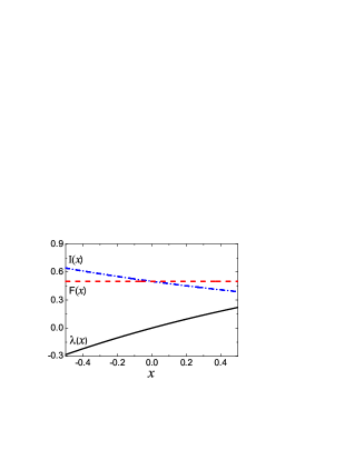
Figure 1: (color online) The LD function $\lambda(x)$, $x$-dependent current $I(x)$ and Fano factor $F(x)$ for transport through a single-level quantum dot. In the symmetric case of $\Gamma_{L}=\Gamma_{R}$ as assumed here, the $x$-independent Fano factor indicates a remarkable scale-invariance fluctuations of the dynamical trajectories.

IV transport through double dots  in parallel

IV.1 Model in a Transformed Representation

In this section we consider a bit more complex setup which consists of a double (quantum) dots (DD) connected in parallel to two leads. Moreover, the interference loop is pierced by a magnetic flux ($\Phi$), similar to the well known Aharonov-Bohm interferometer. It was shown recently that this system has some interesting properties such as a non-analytic current switching behavior, anomalous phase shift, and giant fluctuations of current — all of them induced by the interplay of inter-dot Coulomb correlation and quantum interference LG09 .

Following Ref. LG09 , we assume that each dot has only one level, $E_{1(2)}$, involved in the transport. In large bias limit, for simplicity, we also neglect the spin degrees of freedom, whose effect, under strong Coulomb blockade, can be easily restored by doubling the tunneling rates of each dot with the left lead LG09 . The entire system Hamiltonian reads

$$H=H_{B}+H_{T}+\sum_{\mu=1,2}E_{\mu}a_{\mu}^{\dagger}a_{\mu}+Ua_{1}^{\dagger}a_{1}a_{2}^{\dagger}a_{2}\,.$$ (10)

$a_{1,2}^{\dagger}$ are the creation operators for the DD, and the last term describes the interdot repulsion. The first term, $H_{B}=\sum_{k}[\epsilon_{Lk}b_{Lk}^{\dagger}b_{Lk}+\epsilon_{Rk}b_{Rk}^{\dagger}b_{Rk}]$, is for the leads and $H_{T}$ for their couplings to the dots,

$$H_{T}=\sum_{\mu,k}\Big{(}t_{\mu L}a_{\mu}^{\dagger}b_{Lk}+t_{\mu R}b_{Rk}^{\dagger}a_{\mu}\Big{)}+{\rm H.c.}\,.$$ (11)

Here, we assume that the couplings of the dots to the leads, $t_{\mu L(R)}$, are independent of energy. In the absence of a magnetic field one can always choose the gauge in such a way that all couplings are real. In the presence of a magnetic flux $\Phi$, however, the tunneling amplitudes between the dots and the leads are in general complex. We write $t_{\mu L(R)}={\bar{t}}_{\mu L(R)}e^{i\phi_{\mu L(R)}}$, where $\bar{t}_{\mu L(R)}$ is the coupling without the magnetic field. The phases are constrained to satisfy $\phi_{1L}+\phi_{1R}-\phi_{2L}-\phi_{2R}=\phi$, where $\phi\equiv 2\pi\Phi/\Phi_{0}$. In this work, we only consider the case with strong inter-dot Coulomb blockade($E_{1,2}+U\gg\mu_{L}$)(two dots cannot be both occupied simultaneously).

We found, in Refs. LG09 , that a transformed basis can benefit the analysis a lot. For simplicity, we consider $E_{1}=E_{2}$. In this case, the SU(2) basis transformation reads

$$\left(\begin{array}[]{c}\widetilde{a}_{1}\\ \widetilde{a}_{2}\end{array}\right)={1\over\bar{t}_{R}}\left(\begin{array}[]{cc}t_{1R}&t_{2R}\\ -t^{*}_{2R}&t^{*}_{1R}\end{array}\right)\left(\begin{array}[]{c}a_{1}\\ a_{2}\end{array}\right),$$ (18)

where $\bar{t}_{R}\equiv(\bar{t}_{1R}^{2}+\bar{t}_{2R}^{2})^{1/2}$. Under this transformation, the DD Hamiltonian, $H_{\rm DD}=\sum_{\mu=1,2}E_{\mu}a_{\mu}^{\dagger}a_{\mu}+Ua_{1}^{\dagger}a_{1}a_{2}^{\dagger}a_{2}$, is invariant, while the tunneling Hamiltonian is transformed to

$$H_{T}=\sum_{\mu,k}\Big{(}\widetilde{t}_{\mu L}\widetilde{a}_{\mu}^{\dagger}b_{kL}+\widetilde{t}_{\mu R}b_{kR}^{\dagger}\widetilde{a}_{\mu}\Big{)}+{\rm H.c.}~{},$$ (19)

where, in the transformed basis, the tunneling amplitudes read

$$\widetilde{t}_{1R} = \bar{t}_{R},~{}~{}~{}~{}~{}~{}~{}~{}~{}~{}~{}~{}~{}~{}~{}~{}\widetilde{t}_{2R}=0,$$

$$\widetilde{t}_{1L} = e^{i(\phi_{2L}+\phi_{2R})}(\bar{t}_{1L}\bar{t}_{1R}\,e^{i\phi}+\bar{t}_{2L}\bar{t}_{2R})/\bar{t}_{R},$$

$$\widetilde{t}_{2L} = -e^{i(\phi_{2L}-\phi_{1R})}(\bar{t}_{1L}\bar{t}_{2R}\,e^{i\phi}-\bar{t}_{2L}\bar{t}_{1R})/\bar{t}_{R}.$$ (20)

The advantage of using the transformed basis is thus clear: the state $\widetilde{a}^{\dagger}_{2}|0\rangle$ becomes decoupled with the right lead, and its coupling with the left lead is magnetic-flux tunable (in particular, can be switched off).

IV.2 Large-Deviation Function

In the transformed basis, the strong Coulomb repulsion among the inner dot and inter dots defines a reduced Hilbert space expanded by $\{|0\rangle,|1\rangle,|2\rangle\}$, where $|0\rangle$ stands for the vacant DD state, and $|1(2)\rangle$ for the single occupation state $\widetilde{a}^{\dagger}_{1(2)}|0\rangle$. Using this basis, the number($n$)-dependent master equation reads

$$\dot{\rho}^{(n)}_{00}= -2\Gamma_{L}\rho^{(n)}_{00}+2\Gamma_{R}\rho^{(n-1)}_{11},$$

$$\dot{\rho}^{(n)}_{11}= (1+\cos\phi)\Gamma_{L}\rho^{(n)}_{00}-2\Gamma_{R}\rho^{(n)}_{11},$$

$$\dot{\rho}^{(n)}_{22}= (1-\cos\phi)\Gamma_{L}\rho^{(n)}_{00},$$

$$\dot{\rho}^{(n)}_{12}= i\sin\phi\Gamma_{L}\rho^{(n)}_{00}-\Gamma_{R}\rho^{(n)}_{12},$$

$$\dot{\rho}^{(n)}_{21}= -i\sin\phi\Gamma_{L}\rho^{(n)}_{00}-\Gamma_{R}\rho^{(n)}_{21}.$$ (21)

Here, again, “$n$” is the electron number counted at the right lead. Also, for the sake of brevity, we assumed that $\bar{t}_{1L}=\bar{t}_{2L}=\bar{t}_{L}$, and $\bar{t}_{1R}=\bar{t}_{2R}=\bar{t}_{R}$. Then, the tunneling rates are defined, respectively, as $\Gamma_{L}=2\pi\Omega\bar{t}_{L}^{2}$ and $\Gamma_{R}=2\pi\Omega\bar{t}_{R}^{2}$, with $\Omega$ the density of states of the leads.

Similar to the single dot studied in the preceding section, making the LD transformation, $\rho(x,t)=\sum_{n}\rho^{(n)}(t)e^{-xn}$, and transposing $\rho(x,t)$ into a column-vector form $[\rho_{00},\rho_{11},\rho_{22},\rho_{12},\rho_{21}]^{T}$, we can reexpress Eqs. (IV.2) as $\dot{\rho}(x,t)=-\mathcal{M}(x)\rho(x,t)$, with $\mathcal{M}(x)$ a $5\times 5$ matrix:

$$\mathcal{M}(x)=\begin{pmatrix}2\Gamma_{L}&-2\Gamma_{R}e^{-x}&0&0&0\\ -(1+\cos\phi)\Gamma_{L}&2\Gamma_{R}&0&0&0\\ -(1-\cos\phi)\Gamma_{L}&0&0&0&0\\ -i\sin\phi~{}\Gamma_{L}&0&0&\Gamma_{R}&0\\ i\sin\phi~{}\Gamma_{L}&0&0&0&\Gamma_{R}\end{pmatrix}.$$ (22)

Its eigenvalues read, respectively, $\lambda_{1}=0$, $\lambda_{2(3)}=\Gamma_{R}$, and $\lambda_{4(5)}=(\Gamma_{L}+\Gamma_{R})\pm X$, where $X=\sqrt{(\Gamma_{L}-\Gamma_{R})^{2}+2e^{-x}\Gamma_{L}\Gamma_{R}(1+\cos\phi)}$. Since $\lambda_{2,3,4}$ are positive, we can conclude that the smallest eigenvalue is the smaller one among $\lambda_{1}$ and $\lambda_{5}$. The analysis in Sec. IV (D) will show that, by varying the conjugate field $x$, $\lambda_{5}$ has a crossover from negative to positive, implying that $\lambda_{1}=0$ will suddenly become the smallest eigenvalue. This behavior actually indicates a dynamic phase transition. Before proceeding to such an analysis, for the sake of completeness, in the following we first outline a scheme to account for the dephasing effect between the dots.

IV.3 Dephasing Effect

In real systems, dephasing may originate from surrounding environments, which cause random fluctuations of energy levels. For the present double-dot setup, a controllable dephasing mechanism can be introduced in experiments by performing a “which-path” detection using a nearby quantum point contact (QPC) SG97 ; WM97 ; Buk98 . The dephasing effect of such a “which-path” detection can be accounted for by adding a Lindblad term SG97

$$L_{\phi}\rho^{(n)}L^{\dagger}_{\phi}-\frac{1}{2}L^{\dagger}_{\phi}L_{\phi}\rho^{(n)}-\frac{1}{2}\rho^{(n)}L^{\dagger}_{\phi}L_{\phi},$$ (23)

to the r.h.s of Eq. (IV.2). The pure dephasing operator, $L_{\phi}\equiv\sqrt{\Gamma_{d}}(|1\rangle_{D}\langle 1|-|2\rangle_{D}\langle 2|)$, describes the energy fluctuations of state $|1\rangle_{D}$ and $|2\rangle_{D}$ (in the original basis). Moreover, the dephasing rate can be carried out as SG97 : $\Gamma_{d}=(\sqrt{T}-\sqrt{T^{{}^{\prime}}})^{2}V_{d}/2\pi$, where $V_{d}$ is the bias voltage across the QPC, and $T$ and $T^{{}^{\prime}}$ are the respective transmission probabilities, depending on which dot among the two is occupied. Note also that, since the dephasing does not affect electron’s counting, the above dephasing term is not related to $\rho^{(n-1)}$, but only to $\rho^{(n)}$.

IV.4 Results and Discussions

In the following, we restrict our numerical simulation to a symmetric setup, i.e., $\Gamma_{L}=\Gamma_{R}=\Gamma$, and use $\Gamma$ ($\Gamma^{-1}$ ) as the units of energy (time). For the case of finite counting time ($t_{c}$), applying the scheme described in Sec. II (C), we identify the LD function from $\lambda(x,t_{c})={\cal F}(x,t_{c})/t_{c}$ and simply denote it as $\lambda(x)$. Similar simplified notation will be used also in the following for the $x$-dependent (“$x$-ensemble”) current $I(x)$ and Fano factor $F(x)$.

In Fig. 2 we display the LD function $\lambda(x)$ and the associated $x$-ensemble current $I(x)$. We consider a relatively long counting time $t_{c}=150\Gamma^{-1}$, and assume the dephasing rate $\Gamma_{d}=0.01\Gamma$. Drastically differing from the above result of single dot, here, the LD function (solid lines in Fig. 2) reveals a phase transition behavior, when crossing through a $\phi$-dependent critical point.

To understand this behavior, we refer to the analytic solution obtained in Sec. IV (B), under the ideal case of $\Gamma_{d}=0$. Since the eigenvalues $\lambda_{2,3,4}$ are positive, the smallest eigenvalue, which has dominant contribution to the LD function in long counting-time limit, should be either $\lambda_{1}$ or $\lambda_{5}$, depending on the sign of $\lambda_{5}$. We can easily check that, as a function of the “dynamical field” $x$, $\lambda_{5}$ can be either positive or negative, with a crossover at $x=2\ln|\cos\frac{\phi}{2}|\equiv x_{c}(\phi)$. That is, for $x>x_{c}$, $\lambda_{5}$ is positive, while for $x<x_{c}$ it is negative. This indicates that the LD function $\lambda(x)=0$ for $x>x_{c}$, and $\lambda(x)=\lambda_{5}(x)$ for $x<x_{c}$.

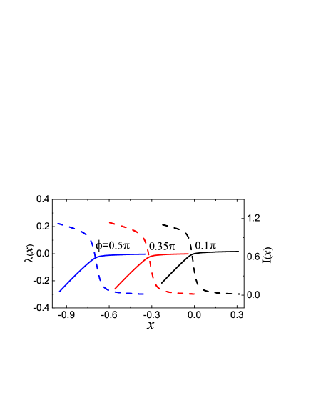
Figure 2: (color online) The LD function $\lambda(x)$ (solid lines) and the $x$-dependent current $I(x)$ (dashed lines) for a double-dot Aharonov-Bohm interferometer in strong Coulomb blockade regime. We assumed a symmetric setup with $\Gamma_{L}=\Gamma_{R}=\Gamma$ and $E_{1}=E_{2}$, a relatively long counting time $t_{c}=150\Gamma^{-1}$, and a dephasing rate $\Gamma_{d}=0.01\Gamma$.

As a further complementary analysis, let us evaluate the distribution function $P(n,t)$ in long time limit. Owing to the assumed Coulomb blockade effect, we know that once the (transformed) upper dot is occupied, i.e., the DD is in the state $\tilde{d}^{\dagger}_{2}|0\rangle$, the current would be completely blocked. Denoting the tunneling probability from the left electrode to the upper (lower) dot as $p_{2(1)}$, the probability with “$n$” electrons transmitted through the DD (actually through the lower dot) simply reads $P(n)=(p_{1})^{n}p_{2}$, before the transport channel is blocked. This distribution function defines the entire ensemble of trajectories, and supports as well a straightforward “subensemble” LD analysis. Noting that $p_{1(2)}=\tilde{\Gamma}_{1(2)L}(\phi)/[\tilde{\Gamma}_{1L}(\phi)+\tilde{\Gamma}_{2L}(\phi)]$, for the symmetric setup $\bar{t}_{1L}=\bar{t}_{2L}=\bar{t}_{L}$ and $\bar{t}_{1R}=\bar{t}_{2R}=\bar{t}_{R}$, we obtain a simple result: $p_{1}=\cos^{2}(\frac{\phi}{2})$, and $p_{2}=\sin^{2}(\frac{\phi}{2})$. Now, let us consider the LD transformation, $P(x)=p_{2}\sum^{\infty}_{n=0}e^{-xn}(p_{1})^{n}$. This infinite series has a convergent sum, $P(x)=\sin^{2}(\frac{\phi}{2})[1-e^{-x}\cos^{2}(\frac{\phi}{2})]^{-1}$, under the condition $e^{-x}\cos^{2}(\frac{\phi}{2})<1$. This convergence condition gives $x>2\ln|\cos(\frac{\phi}{2})|$, implying that the LD function ($\lambda(x)$) is zero in this region, being fully consistent with the result based on the eigenvalue analysis.

In Fig. 2, we also plot the $x$-dependent current $I(x)$, by the solid lines. This re-sampled current over a subensemble of trajectories shows a switching behavior around the particular point $x_{c}(\phi)$. In the ideal case of $E_{1}=E_{2}$, $\Gamma_{d}=0$ and $t_{c}\rightarrow\infty$, the switching behavior of $I(x)$ deforms to a discontinuous jump, owing to the singularity of $\lambda(x)$ at $x_{c}(\phi)$. This feature clearly indicates a first-order dynamical phase transition, revealing a rapid crossover between two distinct dynamical phases across $x_{c}$: an active phase given by $x<x_{c}$ with trajectories having large $n$, and an inactive phase by $x>x_{c}$ with trajectories having small $n$. At the critical point $x_{c}(\phi)$, the two dynamical phases coexist.

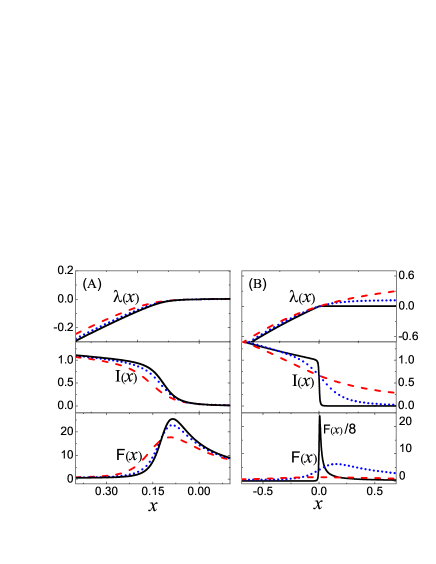
Figure 3: (color online) Effects of the counting time $t_{c}$ and the dot-level offset $\Delta$. In (A), for a given $\Delta=0.1\Gamma$ and $\phi=0.25\pi$, we display the results of $t_{c}=150\Gamma^{-1}$ (blue dotted lines) and $50\Gamma^{-1}$ (red dashed lines) against that of the long $t_{c}$ limit (black solid lines). In (B), in the limits of long counting time and $\phi=0$, we compare the results of $\Delta=0.1\Gamma$ (black solid lines), $0.5\Gamma$ (blue dotted lines) and $\Gamma$ (red dashed lines). In both (A) and (B), we assumed $\Gamma_{L}=\Gamma_{R}=\Gamma$ and $\Gamma_{d}=0$. The latter assumption is mainly for the purpose of showing the pure effects of the counting time and the level offset.

In Fig. 3 (A) and (B) we display, respectively, the effects of the counting time ($t_{c}$) and the dot-level offset ($\Delta$). In Fig. 3 (A), as a comparison to the result of long $t_{c}$ limit (black solid lines), we plot the LD function, the current and the Fano factor for two finite counting times, by the blue dotted and red dashed lines. We see that, as expected, a shorter counting time will result in a milder crossover behavior. As a similar comparison, in Fig. 3(B) we show the effect of the dot-level offset. Since in the transformed basis the two dots are coupled with a tunneling amplitude proportional to $\Delta$, we then understand that the dynamical phase transition will be less drastic as we increase $\Delta$.

V Summary

Starting with a number-conditioned master equation, we formulated an efficient large-deviation approach for mesoscopic transports. Formally, it appears that the large-deviation approach is similar to the FCS. However, a large-deviation analysis is capable of capturing more complete information: not only for the typical trajectories, but also for the rare ones. Through an inspection on the continuous change of subensemble statistics of trajectories, richer dynamical behaviors can be revealed. Methodologically, in addition to the eigenvalues analysis in long time limit, we also presented a convenient scheme of calculating the large-deviation function for arbitrary counting times.

As illustrative applications, we considered two examples: one is the transport through a single dot, another is through a double dots. Even for the simple system of single dot, we found that the symmetry of the tunnel coupling to the leads would strongly affect the statistics of the trajectories, which is indeed outside the scope of the usual FCS analysis. Very interestingly, similar to the “unexpected” finding uncovered in the quantum optical system of driving two-level atoms Gar10 , here a symmetric tunnel-coupling in our single-dot transport system can as well result in a (“time” or “tunneling-rate”) scale-invariance behavior in the statistics of trajectories. For the double-dot setup, our large-deviation analysis reveals a more profound behavior, say, the dynamical phase transition, which is, essentially, induced by the Coulomb correlation and quantum interference, and were analyzed in detail by combining numerical simulations with some analytic solutions.

The large-deviation approach, owing to its ability to analyze the subensemble statistics of trajectories, is anticipated to apply to various scenarios, e.g., from electronic nano-devices to femtochemistry. In particular, its systematic applications to important mesoscopic transport systems are extremely promising, which is seemingly a new area waiting for exploitation.

Acknowledgments.— This work was supported by the NNSF of China under grants No. 101202101 & 10874176, and the Major State Basic Research Project.

References

- (1) Ya. M. Blanter and M. Büttiker, Phys. Rep. 336, 1 (2000); Quantum Noise in Mesoscopic Physics, edited by Yu. V. Nazarov (Kluwer, Dordrecht, 2003).
- (2) L. S. Levitov and G. B. Lesovik, JETP Lett. 58, 230 (1993); L. S. Levitov, H. W. Lee, and G. B. Lesovik, J. Math. Phys. 37, 4845 (1996).
- (3) W. Belzig and Yu. V. Nazarov, Phys. Rev. Lett. 87, 067006 (2001); W. Belzig and Yu. V. Nazarov, Phys. Rev. Lett. 87, 197006 (2001).
- (4) P. Samuelsson and M. Büttiker, Phys. Rev. Lett. 89, 046601 (2002); Phys. Rev. B 66, 201306 (2002).
- (5) S. Pilgram and P. Samuelsson, Phys. Rev. Lett. 94, 086806 (2005).
- (6) A. Thielmann, M. H. Hettler, J. König, and G. Schön, Phys. Rev. B 71, 045341 (2005); J. Aghassi, A. Thielmann, M. H. Hettler, and G. Schön, ibid. 73, 195323 (2006); A. Thielmann, M. H. Hettler, J. König, and G. Schön, Phys. Rev. Lett. 95, 146806 (2005).
- (7) W. Belzig, Phys. Rev. B 71, 161301(R) (2005).
- (8) B. R. Bulka, Phys. Rev. B 62, 1186 (2000).
- (9) A. Cottet, W. Belzig, and C. Bruder, Phys. Rev. Lett. 92, 206801 (2004).
- (10) Ya. M. Blanter, O. Usmani, and Yu. V. Nazarov, Phys. Rev. Lett. 93, 136802 (2004).
- (11) T. Novotny, A. Donarini, C. Flindt, and A.-P. Jauho, Phys. Rev. Lett. 92, 248302 (2004).
- (12) C. W. Groth, B. Michaelis, and C. W. J. Beenakker, Phys. Rev. B 74, 125315 (2006).
- (13) S. K. Wang, H. J. Jiao, F. Li, X. Q. Li, and Y. J. Yan, Phys. Rev. B 76, 125416 (2007).
- (14) S. Gustavsson, R. Leturcq, B. Simovič, R. Schleser, T. Ihn, P. Studerus, K. Ensslin, D. C. Driscoll, and A. C. Gossard, Phys. Rev. Lett. 96, 076605 (2006).
- (15) S. Datta, Electronic Transport in Mesoscopic Systems (Cambridge University Press, New York, 1995).
- (16) H. Haug and A.-P. Jauho, Quantum Kinetics in Transport and Optics of Semiconductors (Springer-Verlag, Berlin, 1996).
- (17) S. A. Gurvitz and Ya. S. Prager, Phys. Rev. B 53, 15932 (1996).
- (18) A. Shnirman and G. Schön, Phys. Rev. B 57, 15400 (1998); Yu. Makhlin, G. Schön, and A. Shnirman, Rev. Mod. Phys. 73, 357 (2001).
- (19) X. Q. Li, P. Cui, and Y. J. Yan, Phys. Rev. Lett. 94, 066803 (2005). X. Q. Li, J. Luo, Y. G. Yang, P. Cui, and Y. J. Yan, Phys. Rev. B 71, 205304 (2005).
- (20) D. Mozyrsky and I. Martin, Phys. Rev. Lett. 89, 018301 (2002).
- (21) S. A. Gurvitz, L. Fedichkin, D. Mozyrsky, and G. P. Berman, Phys. Rev. Lett. 91, 066801 (2003).
- (22) C. Flindt, T. Novotny, and A. P. Jauho, Europhys. Lett. 69, 475 (2005).
- (23) J.-P. Eckmann and D. Ruelle, Rev. Mod. Phys. 57, 617 (1985); P. Gaspard, Chaos, Scattering and Statistical Mechanics (Cambridge University Press, Cambridge, England, 1998); H. Touchette, Phys. Rep. 478, 1 (2009).
- (24) D. Chandler, Introduction to Modern Statistical Mechanics (Oxford University Press, Oxford, 1987); N. Goldenfeld, Lectures on Phase Transitions and the Renormalization Group (Westview Press, Boulder, 1992).
- (25) J. P. Garrahan and I. Lesanovsky, Phys. Rev. Lett. 104, 160601 (2010).
- (26) Y. J. Yan, Phys. Rev. A 58, 2721 (1998).
- (27) R. X. Xu, P. Cui, X. Q. Li, Y. Mo, and Y. J. Yan, J. Chem. Phys. 122, 041103 (2005); X. Zheng, J. S. Jin, and Y. J. Yan, New J. Phys. 10, 093016 (2008).
- (28) F. Li, X. Q. Li, W. M. Zhang and S. Gurvitz, Europhys. Lett. 88, 37001(2009); F. Li, H. J. Jiao, J. Y. Luo, H. Wang, and X. Q. Li, Physica E 41, 521 (2009); F. Li, H. J. Jiao, J. Y. Luo, X. Q. Li, and S. A. Gurvitz, ibid. 41, 1707 (2009).
- (29) S. A. Gurvitz, Phys. Rev. B 56, 15 215 (1997).
- (30) I. L. Aleiner, N. S. Wingreen, and Y. Meir, Phys. Rev. Lett. 79, 3740 (1997).
- (31) E. Buks, R. Schuster, M. Heiblum, D. Mahalu, and V. Umansky, Nature (London) 391, 871 (1998).