Measurement of branching ratio and $B_{s}^{0}$ lifetime in the decay $B_{s}^{0}\rightarrow J\!/\!\psi f_{0}(980)$ at CDF

Abstract

We present a study of $B_{s}^{0}$ decays to the CP-odd final state $J\!/\!\psi f_{0}(980)$ with $J\!/\!\psi\rightarrow\mu^{+}\mu^{-}$ and $f_{0}(980)\rightarrow\pi^{+}\pi^{-}$. Using $p\bar{p}$ collision data with an integrated luminosity of $3.8$ $\mathrm{fb^{-1}}$ collected by the CDF II detector at the Tevatron we measure a $B_{s}^{0}$ lifetime of $\tau(B_{s}^{0}\rightarrow J\!/\!\psi f_{0}(980))=1.70_{-0.11}^{+0.12}(\mathrm{stat})\pm 0.03(\mathrm{syst})\,\mathrm{ps}$. This is the first measurement of the $B_{s}^{0}$ lifetime in a decay to a CP eigenstate and corresponds in the standard model to the lifetime of the heavy $B_{s}^{0}$ eigenstate. We also measure the product of branching fractions of $B_{s}^{0}\rightarrow J\!/\!\psi f_{0}(980)$ and $f_{0}(980)\rightarrow\pi^{+}\pi^{-}$ relative to the product of branching fractions of $B_{s}^{0}\rightarrow J\!/\!\psi\phi$ and $\phi\rightarrow K^{+}K^{-}$ to be $R_{f_{0}/\phi}=0.257\pm 0.020(\mathrm{stat})\pm 0.014(\mathrm{syst})$, which is the most precise determination of this quantity to date.

I Introduction

In the standard model, the mass and flavor eigenstates of the $B_{s}^{0}$ meson are not identical. This gives rise to particle – anti-particle oscillations Gay:2001ra , which proceed in the standard model through second order weak interaction processes, and whose phenomenology depends on the Cabibbo-Kobayashi-Maskawa (CKM) quark mixing matrix. The time $(t)$ evolution of $B_{s}^{0}$ mesons is approximately governed by the Schrödinger equation

$$i\frac{d}{dt}\left(\begin{array}[]{c}|B_{s}^{0}(t)\rangle\\ |\bar{B}_{s}^{0}(t)\rangle\end{array}\right)=\left(\hat{M}^{s}-\frac{i}{2}\hat{\Gamma}^{s}\right)\left(\begin{array}[]{c}|B_{s}^{0}(t)\rangle\\ |\bar{B}_{s}^{0}(t)\rangle\end{array}\right),$$ (1)

where $\hat{M}^{s}$ and $\hat{\Gamma}^{s}$ are mass and decay rate symmetric $2\times 2$ matrices. Diagonalization of $\hat{M}^{s}-\frac{i}{2}\hat{\Gamma}^{s}$ leads to mass eigenstates

$$|B_{sL}^{0}\rangle = p\;|B_{s}^{0}\rangle+q\;|\bar{B}_{s}^{0}\rangle,$$ (2)

$$|B_{sH}^{0}\rangle = p\;|B_{s}^{0}\rangle-q\;|\bar{B}_{s}^{0}\rangle,$$ (3)

with distinct masses ($M_{s}^{L},\,M_{s}^{H}$) and distinct decay rates ($\Gamma_{s}^{L},\,\Gamma_{s}^{H}$), where $p$ and $q$ are complex numbers satisfying $|p|^{2}+|q|^{2}=1$. An important feature of the $B_{s}^{0}$ system is the non-zero matrix element $\Gamma_{12}^{s}$ representing the partial width of $B_{s}^{0}$ and $\bar{B}_{s}^{0}$ decays to common final states which translates into a non-zero decay width difference $\Delta\Gamma_{s}$ of the two mass eigenstates through the relation

$$\Delta\Gamma_{s} = \Gamma_{s}^{L}-\Gamma_{s}^{H}=2|\Gamma_{12}^{s}|\cos\phi_{s},$$ (4)

where $\phi_{s}=\mbox{arg}(-M_{12}^{s}/\Gamma_{12}^{s})$. The phase $\phi_{s}$ describes CP violation in $B_{s}^{0}$ mixing. In the standard model $\phi_{s}$ is predicted to be $0.22^{\circ}\pm 0.06^{\circ}$ Lenz:2006hd ; Nierste:2011ti . The small value of the phase $\phi_{s}$ causes the mass and CP eigenstates to coincide to a good approximation. Thus the measurement of the lifetime in a CP eigenstate provides directly the lifetime of the corresponding mass eigenstate. If new physics is present, it could enhance $\phi_{s}$ to large values, a scenario which is not excluded by current experimental constraints. In such a case the correspondence between mass and CP eigenstates does not hold anymore and the measured lifetime will correspond to the weighted average of the lifetimes of the two mass eigenstates with weights dependent on the size of the CP violating phase $\phi_{s}$ Dunietz:2000cr . Thus a measurement of the $B_{s}^{0}$ lifetime in a final state which is a CP eigenstate provides, in combination with other measurements, valuable information on the decay width difference $\Delta\Gamma_{s}$ and the CP violation in $B_{s}^{0}$ mixing.

One of the most powerful measurements to constrain a new physics contribution to the phase $\phi_{s}$ is the measurement of CP violation in the decay $B_{s}^{0}\rightarrow J\!/\!\psi\phi$ with $\phi\rightarrow K^{+}K^{-}$. The decay $B_{s}^{0}\rightarrow J\!/\!\psi\phi$ has a mixture of the CP-even and -odd components in the final state and an angular analysis is needed to separate them Dighe:1995pd . In the standard model, CP violation in the decay $B_{s}^{0}\rightarrow J\!/\!\psi\phi$ is given by $\beta_{s}=\arg[({-V_{ts}V_{tb}^{*}})/({V_{cs}V_{cb}^{*}})]$. New physics effects in $B_{s}^{0}$ mixing would shift $\phi_{s}$ and $-2\beta_{s}$ from the standard model value by the same amount. A sufficiently copious $B_{s}^{0}\rightarrow J\!/\!\psi f_{0}$ signal with $f_{0}\rightarrow\pi^{+}\pi^{-}$, where $f_{0}$ stands for $f_{0}(980)$, and $B_{s}^{0}$ flavor identified at production can be used to measure $\beta_{s}$ without the need of an angular analysis Stone:2009hd as $J\!/\!\psi f_{0}$ is a pure CP-odd final state. Since the $B_{s}^{0}$ is a spin 0 particle and the decay products $J\!/\!\psi$ and $f_{0}$ have quantum numbers $J^{PC}=1^{--}$ and $0^{++}$, respectively, the final state has an orbital angular momentum of $L=1$ leading to a CP eigenvalue of $(-1)^{L}=-1$. Further interest in the decay $B_{s}^{0}\rightarrow J\!/\!\psi f_{0}$ arises from its possible contribution to an $S$-wave component in the $B_{s}^{0}\rightarrow J\!/\!\psi K^{+}K^{-}$ decay if the $f_{0}$ decays to $K^{+}K^{-}$. This contribution could help to resolve an ambiguity in the $\Delta\Gamma_{s}$ and $\beta_{s}$ values determined in the $B_{s}^{0}\rightarrow J\!/\!\psi\phi$ analyses. Because it was neglected in the first tagged $B_{s}^{0}\rightarrow J\!/\!\psi\phi$ results Aaltonen:2007he ; Abazov:2008fj , each of which showed an approximately 1.5 $\sigma$ deviation from the standard model, it was argued that the omission may significantly bias the results Stone:2008ak ; Stone:2010dp . However, using the formalism in Ref. Azfar:2010nz , the latest preliminary CDF measurement beta_s has shown that the $S$-wave interference effect is negligible at the current level of precision.

In Refs. Lenz:2006hd ; Nierste:2011ti the decay width difference in the standard model is predicted to be $\Delta\Gamma_{s}^{\rm SM}=(0.087\pm 0.021)$ ps^-1 and the ratio of the average $B_{s}^{0}$ lifetime, $\tau_{s}=2/(\Gamma_{s}^{L}+\Gamma_{s}^{H})$, to the $B^{0}$ lifetime, $\tau_{d}$, to be $0.996<\tau_{s}/\tau_{d}<1$. Using these predictions in the relations

$$\Gamma_{s}^{H} = \frac{1}{\tau_{s}^{H}}=\Gamma_{s}-\frac{1}{2}\Delta\Gamma_{s},$$ (5)

$$\Gamma_{L}^{s} = \frac{1}{\tau_{s}^{L}}=\Gamma_{s}+\frac{1}{2}\Delta\Gamma_{s},$$ (6)

where $\Gamma_{s}=1/\tau_{s}$, together with the world average $B^{0}$ lifetime, $\tau_{d}=(1.525\pm 0.009)$ ps Nakamura:2010zzi , we find the theoretically-derived values $\tau_{s}^{H}=(1.630\pm 0.030)$ ps and $\tau_{s}^{L}=(1.427\pm 0.023)$ ps.

While no direct measurements of $B_{s}^{0}$ lifetimes in decays to pure CP eigenstates are available, various experimental results allow for the determination of the lifetimes of the two mass eigenstates. Measurements sensitive to these lifetimes are the angular analysis of $B_{s}^{0}\rightarrow J\!/\!\psi\phi$ decays and the branching fraction of $B_{s}^{0}\rightarrow D_{s}^{(*)+}D_{s}^{(*)-}$, which can be complemented by measurements of the $B_{s}^{0}$ lifetime in flavor specific final states. The combination of available measurements yields $\tau_{s}^{H}=(1.544\pm 0.041)$ ps and $\tau_{s}^{L}=(1.407^{+0.028}_{-0.026})$ ps Asner:2010qj . From CDF measurements we can infer the two lifetimes from the result of the angular analysis of $B_{s}^{0}\rightarrow J\!/\!\psi\phi$ decays. The latest preliminary result beta_s , that is not yet included in the above average, yields $\tau_{s}^{H}=(1.622\pm 0.068)$ ps and $\tau_{s}^{L}=(1.446\pm 0.035)$ ps assuming standard model CP violation.

Compared to measurements using $B_{s}^{0}\rightarrow J\!/\!\psi\phi$ decays, lifetime and future CP violation measurements in the $B_{s}^{0}\rightarrow J\!/\!\psi f_{0}$ decay suffer from a lower branching fraction. Based on a comparison to $D_{s}^{+}$ meson decays Ref. Stone:2008ak makes a prediction for the branching fraction of $B_{s}^{0}\rightarrow J\!/\!\psi f_{0}$ decay relative to the $B_{s}^{0}\rightarrow J\!/\!\psi\phi$ decay,

$$R_{f_{0}/\phi}=\frac{\mathcal{B}(B_{s}^{0}\rightarrow J\!/\!\psi f_{0})}{\mathcal{B}(B_{s}^{0}\rightarrow J\!/\!\psi\phi)}\frac{\mathcal{B}(f_{0}\rightarrow\pi^{+}\pi^{-})}{\mathcal{B}(\phi\rightarrow K^{+}K^{-})},$$ (7)

to be approximately 0.2. The CLEO experiment estimates $R_{f_{0}/\phi}=0.42\pm 0.11$ from a measurement of semileptonic $D_{s}^{+}$ decays Ecklund:2009fia . A theoretical prediction based on QCD factorization yields a range of $R_{f_{0}/\phi}$ between $0.2$ and $0.5$ Leitner:2010fq . With the world average branching fraction for the $B_{s}^{0}\rightarrow J\!/\!\psi\phi$ decay of $(1.3\pm 0.4)\times 10^{-3}$ and the branching fraction of $f_{0}\rightarrow\pi^{+}\pi^{-}$ in the region between 0.5–0.8, predictions of $\mathcal{B}(B_{s}^{0}\rightarrow J\!/\!\psi f_{0})$ Colangelo:2010bg ; Colangelo:2010wg translate into a wide range of $R_{f_{0}/\phi}$ values of approximately 0.1–0.5.

The first experimental search was performed by the Belle experiment Louvot:2010es . Their preliminary result did not yield a signal and they extract an upper limit on the branching fraction of $\mathcal{B}(B_{s}^{0}\rightarrow J\!/\!\psi f_{0})\mathcal{B}(f_{0}\rightarrow\pi^{+}\pi^{-})<1.63\times 10^{-4}\;\mathrm{at\;90\%\;C.L}$. Recently the LHCb experiment reported the first observation of the decay $B_{s}^{0}\rightarrow J\!/\!\psi f_{0}$ Aaij:2011fx with a relative branching fraction of $R_{f_{0}/\phi}=0.252^{+0.046}_{-0.032}(\mathrm{stat})\,^{+0.027}_{-0.033}(\mathrm{syst})$. Shortly after the LHCb result was presented, the Belle collaboration announced their result of an updated analysis using 121.4 $\mathrm{fb^{-1}}$ of $\Upsilon(5S)$ data Li:2011pg . They observe a significant $B_{s}^{0}\rightarrow J\!/\!\psi f_{0}$ signal and measure $\mathcal{B}(B_{s}^{0}\rightarrow J\!/\!\psi f_{0})\mathcal{B}(f_{0}\rightarrow\pi^{+}\pi^{-})=(1.16^{+0.31}_{-0.19}\,{}^{+0.15}_{-0.17}\,{}^{+0.26}_{-0.18})\times 10^{-4}$, where the first uncertainty is statistical, the second systematic, and the third one is an uncertainty on the number of produced $B_{s}^{(*)0}\bar{B}_{s}^{(*)0}$ pairs. Using their preliminary measurement of the $B_{s}^{0}\rightarrow J\!/\!\psi\phi$ branching fraction Louvot:2009xg , and assuming that the uncertainty on the number of produced $B_{s}^{(*)0}\bar{B}_{s}^{(*)0}$ pairs is fully correlated for the two measurements, this translates into $R_{f_{0}/\phi}=0.206^{+0.055}_{-0.034}(\mathrm{stat})\pm 0.052(\mathrm{syst})$. A preliminary measurement of the D0 experiment yields $R_{f_{0}/\phi}=0.210\pm 0.032(\mathrm{stat})\pm 0.036(\mathrm{syst})$ D0:6152 .

In this paper we present a measurement of the ratio $R_{f_{0}/\phi}$ of the branching fraction of the $B_{s}^{0}\rightarrow J\!/\!\psi f_{0}$ decay relative to the $B_{s}^{0}\rightarrow J\!/\!\psi\phi$ decay and the first measurement of the $B_{s}^{0}$ lifetime in a decay to a pure CP eigenstate. We use data collected by the CDF II detector from February 2002 until October 2008. The data correspond to an integrated luminosity of $3.8\>\mbox{fb}^{-1}$.

This paper is organized as follows: In Sec. II we describe the CDF II detector together with the online data selection, followed by the candidate selection in Sec. III. Section IV describes details of the measurement of the ratio $R_{f_{0}/\phi}$ of branching fractions of the $B_{s}^{0}\rightarrow J\!/\!\psi f_{0}$ decay relative to the $B_{s}^{0}\rightarrow J\!/\!\psi\phi$ decay while Sec. V discusses the lifetime measurement. We finish with a short discussion of the results and conclusions in Sec. VI.

II CDF II detector and trigger

Among the components of the CDF II detector Acosta:2004yw the tracking and muon detection systems are most relevant for this analysis. The tracking system lies within a uniform, axial magnetic field of $1.4$ T strength. The inner tracking volume hosts 7 layers of double-sided silicon micro-strip detectors up to a radius of $28$ cm Hill:2004qb . An additional layer of single-sided silicon is mounted directly on the beam-pipe at a radius of $1.5$ cm, providing an excellent resolution of the impact parameter $d_{0}$, defined as the distance of closest approach of the track to the interaction point in the transverse plane. The silicon tracker provides a pseudorapidity coverage up to $|\eta|\leq 2.0$. The remainder of the tracking volume up to a radius of $137$ cm is occupied by an open-cell drift chamber Affolder:2003ep . The drift chamber provides up to 96 measurements along the track with half of them being axial and other half stereo. Tracks with $|\eta|\leq 1.0$ pass the full radial extent of the drift chamber. The integrated tracking system achieves a transverse momentum resolution of $\sigma(p_{T})/p^{2}_{T}\approx 0.07\%$ (GeV$/c$)^-1 and an impact parameter resolution of $\sigma(d_{0})\approx 35$ $\mathrm{\mu m}$ for tracks with a transverse momentum greater than 2 $\mathrm{GeV}/c$. The tracking system is surrounded by electromagnetic and hadronic calorimeters, which cover the full pseudorapidity range of the tracking system Balka:1987ty ; Bertolucci:1987zn ; Albrow:2001jw ; Apollinari:1998bg . We detect muons in three sets of multi-wire drift chambers. The central muon detector has a pseudorapidity coverage of $|\eta|<0.6$ Ascoli:1987av and the calorimeters in front of it provide about 5.5 interaction lengths of material. The minimum transverse momentum to reach this set of muon chambers is about 1.4 $\mathrm{GeV}/c$. The second set of chambers covers the same range in $\eta$, but is located behind an additional 60 cm of steel absorber, which corresponds to about 3 interaction lengths. It has a higher transverse momentum threshold of 2 $\mathrm{GeV}/c$, but provides a cleaner muon identification. The third set of muon detectors extends the coverage to a region of $0.6<|\eta|<1.0$ and is shielded by about 6 interaction lengths of material.

A three-level trigger system is used for the online event selection. The trigger component most important for this analysis is the extremely fast tracker (XFT) Thomson:2002xp , which at the first level groups hits from the drift chamber into tracks in the plane transverse to the beamline. Candidate events containing $J\!/\!\psi\rightarrow\mu^{+}\mu^{-}$ decays are selected by a dimuon trigger Acosta:2004yw which requires two tracks of opposite charge found by the XFT that match to track segments in the muon chambers and have a dimuon invariant mass in the range 2.7 to 4.0 GeV/$c^{2}$.

III Reconstruction and candidate selection

III.1 Reconstruction

In the offline reconstruction we first combine two muon candidates of opposite charge to form a $J\!/\!\psi$ candidate. We consider all tracks that can be matched to a track segment in the muon detectors as muon candidates. The $J\!/\!\psi$ candidate is subject to a kinematic fit with a vertex constraint. We then combine the $J\!/\!\psi$ candidate with two other oppositely charged tracks that are assumed to be pions and have an invariant mass between 0.85 and 1.2 $\mathrm{GeV}/c^{2}$ to form a $B_{s}^{0}\rightarrow J\!/\!\psi f_{0}$ candidate. In the final step a kinematic fit of the $B_{s}^{0}\rightarrow J\!/\!\psi f_{0}$ candidate is performed. In this fit we constrain all four tracks to originate from a common vertex, and the two muons forming the $J\!/\!\psi$ are constrained to have an invariant mass equal to the world average $J\!/\!\psi$ mass Nakamura:2010zzi . In a similar way we also reconstruct $B_{s}^{0}\rightarrow J\!/\!\psi\phi$ candidates using pairs of tracks of opposite charge assumed to be kaons and having an invariant mass between 1.009 and 1.029 $\mathrm{GeV}/c^{2}$. During the reconstruction we place minimal requirements on the track quality, the quality of the kinematic fit, and the transverse momentum of the $B_{s}^{0}$ candidate to ensure high quality measurements of properties for each candidate. For the branching fraction measurement we add a requirement which aims at removing a large fraction of short-lived background. We require the decay time of the $B_{s}^{0}$ candidate in its own rest frame, the proper decay time, to be larger than three times its uncertainty. This criterion is not imposed in the lifetime analysis since it would bias the lifetime distribution. The proper decay time is determined by the expression

$$t=\frac{L_{xy}\cdot m(B_{s}^{0})}{c\cdot p_{T}}$$ (8)

where $L_{xy}$ is the flight distance projected onto the $B_{s}^{0}$ momentum in the plane transverse to the beamline, $p_{T}$ is the transverse momentum of the given candidate, and $m(B_{s}^{0})$ is the reconstructed mass of the $B_{s}^{0}$ candidate. The uncertainty on the proper decay time $t$ is estimated for each candidate by propagating track parameter and primary vertex uncertainties into an uncertainty on $L_{xy}$. The proper decay time resolution is typically of the order of 0.1 ps.

III.2 Selection

The selection is performed using a neural network based on the neurobayes package Feindt:2006pm ; Feindt:2004aa . The neural network combines several input variables to form a single output variable on which the selection is performed. The transformation from the multidimensional space of input variables to the single output variable is chosen during a training phase such that it maximizes the separation between signal and background distributions. For each of the two measurements presented in this paper we use a specialized neural network. For the training we need two sets of events with a known classification of signal or background. For the signal sample we use simulated events. We generate the kinematic distributions of $B_{s}^{0}$ mesons according to the measured $b$-hadron momentum distribution. The decay of the generated $B_{s}^{0}$ particles into the $J\!/\!\psi f_{0}$ final state is simulated using the evtgen package Lange:2001uf . Each event is passed through the standard CDF II detector simulation, based on the geant3 package Brun:1978fy ; Gerchtein:2003ba . The simulated events are reconstructed with the same reconstruction software as real data events. The background sample is taken from data using candidates with the $J\!/\!\psi\pi^{+}\pi^{-}$ invariant mass above the $B_{s}^{0}$ signal peak, where only combinatorial background events contribute. Because the requirement on the proper decay time significance efficiently suppresses background events in the branching ratio measurement, we use an enlarged sideband region of 5.45 to 5.55 $\mathrm{GeV}/c^{2}$ in this analysis, compared to an invariant mass range from 5.45 to 5.475 $\mathrm{GeV}/c^{2}$ for the lifetime measurement.

For the branching fraction measurement, the inputs to the neural network, ordered by the importance of their contribution to the discrimination power, are the transverse momentum of the $f_{0}$, the $\chi^{2}$ of the kinematic fit of the $B_{s}^{0}$ candidate using information in the plane transverse to the beamline, the proper decay time of the $B_{s}^{0}$ candidate, the quality of the kinematic fit of the $B_{s}^{0}$ candidate, the helicity angle of the positive pion, the transverse momentum of the $B_{s}^{0}$ candidate, the quality of the kinematic fit of the two pions with a common vertex constraint, the helicity angle of the positive muon, and the quality of the kinematic fit of the two muons with common vertex constraint. The helicity angle of the muon (pion) is defined as the angle between the three momenta of the muon (pion) and $B_{s}^{0}$ candidate measured in the rest frame of the $J\!/\!\psi$ ($f_{0}$). For the selection of $B_{s}^{0}\rightarrow J\!/\!\psi\phi$ decays we use the same neural network without retraining and simply replace $f_{0}$ variables by $\phi$ variables and pions by kaons.

For the lifetime measurement we modify the list of inputs by removing the proper decay time. We also do not use the helicity angles as they provide almost no additional separation power on the selected sample. Since we are not concerned about a precise efficiency determination for the lifetime measurement, we add the following inputs: the invariant mass of the two pions, the likelihood based identification information for muons Thesis:Giurgiu , and the invariant mass of the muon pair. The muon identification is based on the matching of tracks from the tracking system to track segments in the muon system, energy deposition in the electromagnetic and hadronic calorimeters, and isolation of the track. The isolation is defined as the transverse momentum carried by the muon candidate over the scalar sum of transverse momenta of all tracks in a cone of $\Delta R=\sqrt{(\Delta\phi)^{2}+(\Delta\eta)^{2}}<0.4$, where $\Delta\phi$ ($\Delta\eta$) is the difference in azimuthal angle (pseudorapidity) of the muon candidate and the track. There is no significant change in the importance ordering of the inputs. The invariant mass of the pion pair becomes the second most important input, the likelihood based identification of the two muon candidates is ranked fourth and sixth in the importance list, and the muon pair invariant mass is the least important input.

For the branching fraction measurement we select the threshold on the neural network output by maximizing $\epsilon/(2.5+\sqrt{N_{b}})$ Punzi:2003bu , where $\epsilon$ is the reconstruction efficiency for $B_{s}^{0}\rightarrow J\!/\!\psi f_{0}$ decays and $N_{b}$ is the number of background events estimated from the $J\!/\!\psi\pi^{+}\pi^{-}$ mass sideband. The invariant mass distributions of selected $B_{s}^{0}\rightarrow J\!/\!\psi f_{0}$ and $B_{s}^{0}\rightarrow J\!/\!\psi\phi$ candidates are shown in Figs. 1 and 2. A clear signal at around 5.36 $\mathrm{GeV}/c^{2}$ is visible in both mass distributions.

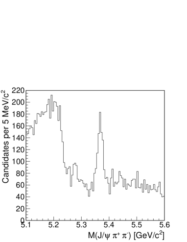
Figure 1: The invariant mass distribution of $B_{s}^{0}\rightarrow J\!/\!\psi f_{0}$ candidates selected for the branching fraction measurement.

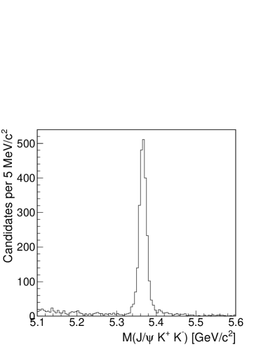
Figure 2: The invariant mass distribution of $B_{s}^{0}\rightarrow J\!/\!\psi\phi$ candidates selected for the branching fraction measurement.

For the lifetime measurement we use simulated experiments to determine the optimal neural network output requirement. We select a value that minimizes the statistical uncertainty of the measured lifetime. We scan a wide range of neural network output values and for each requirement we simulate an ensemble of experiments with a $B_{s}^{0}$ lifetime of 1.63 ps, where the number of signal and background events as well as the background distributions are simulated according to data. For a broad range of selection requirements we observe the same uncertainty within a few percent. Our final requirement on the network output is chosen from the central region of this broad range of equivalent options.

III.3 Physics backgrounds

We study possible physics backgrounds using simulated events with all $b$-hadrons produced and decayed inclusively to final states containing a $J\!/\!\psi$. For this study we use the selection from the branching fraction measurement. While several physics backgrounds appear in the $J\!/\!\psi\pi^{+}\pi^{-}$ mass spectrum, none contributes significantly under the $B_{s}^{0}$ peak. The most prominent physics backgrounds are $B^{0}\rightarrow J\!/\!\psi K^{*0}$ with $K^{*0}\rightarrow K^{+}\pi^{-}$, where $K^{*0}$ stands for $K^{*}(892)^{0}$, and $B^{0}\rightarrow J\!/\!\psi\pi^{+}\pi^{-}$. In the first case the kaon is mis-reconstructed as a pion and gives rise to a large fraction of the structure seen below 5.22 $\mathrm{GeV}/c^{2}$, while the second one is correctly reconstructed and produces the narrow peak at approximately 5.28 $\mathrm{GeV}/c^{2}$. Another possible physics type of background would consist of properly reconstructed $B^{+}$ combined with a random track. This type of background would contribute only to higher masses with a threshold above the $B_{s}^{0}$ signal. As we do not find evidence of such background in Ref. Aaltonen:2011sy which is more sensitive we conclude that this kind of background is also negligible here. The stacked histogram of physics backgrounds derived from simulation is shown in Fig. 3. From this study we conclude that the main physics background that has to be included as a separate component in a fit to the mass spectrum above 5.26 $\mathrm{GeV}/c^{2}$ stems from decays of $B^{0}\rightarrow J\!/\!\psi\pi^{+}\pi^{-}$. It is properly reconstructed and therefore simple to parametrize. All other physics backgrounds are negligible.

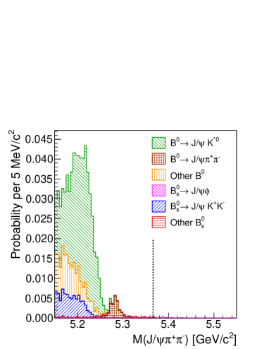
Figure 3: (color online) Stacked histogram of physics backgrounds to $B_{s}^{0}\rightarrow J\!/\!\psi f_{0}$ derived from simulation using the selection for the branching fraction measurement. The vertical line indicates the location of the world average $B_{s}^{0}$ mass.

IV Branching fraction measurement

In this Section we describe details of the branching fraction measurement. These involve the maximum likelihood fit to extract the number of signal events, the efficiency estimation, and the systematic uncertainties. We conclude this Section with the result for the ratio $R_{f_{0}/\phi}$ of branching fractions between $B_{s}^{0}\rightarrow J\!/\!\psi f_{0}$ and $B_{s}^{0}\rightarrow J\!/\!\psi\phi$ decays.

IV.1 Fit description

We use an unbinned extended maximum likelihood fit of the invariant mass to extract the number of $B_{s}^{0}$ decays in our samples. In order to avoid the need for modeling most of the physics background, we restrict the fit to the mass range from 5.26 $\mathrm{GeV}/c^{2}$ to 5.5 $\mathrm{GeV}/c^{2}$. The likelihood is

$$\mathcal{L}=\prod_{i=1}^{N} \left[N_{s}\cdot P_{s}(m_{i})+N_{cb}\cdot P_{cb}(m_{i})+\right.$$ (9)

$$\left.f_{pb}\cdot N_{s}\cdot P_{pb}(m_{i})+N_{B^{0}}\cdot P_{B^{0}}(m_{i})\right]\cdot$$

$$e^{-(N_{s}+N_{cb}+N_{s}\cdot f_{pb}+N_{B^{0}})},$$

where $m_{i}$ is the invariant mass of the $i$-th candidate and $N$ is the total number of candidates in the sample. The fit components are denoted by the subscripts $s$ for signal, $cb$ for combinatorial background, $pb$ for physics background, and $B^{0}$ for $B^{0}\rightarrow J\!/\!\psi\pi^{+}\pi^{-}$ background. The yields of the components are given by $N_{s}$, $N_{cb}$, $N_{s}\cdot f_{pb}$, and $N_{B^{0}}$, and their probability density functions (PDFs) by $P_{s,cb,pb,B^{0}}(m_{i})$, respectively. The physics background yield is parametrized relative to the signal yield via the ratio $f_{pb}$ to allow constraining it by other measurements in the $B_{s}^{0}\rightarrow J\!/\!\psi\phi$ fit.

The signal PDF $P_{s}(m_{i})$ is parametrized by a sum of two Gaussian functions with a common mean. The relative size of the two Gaussians and their widths are determined from simulated events. Approximately 82% of the $B_{s}^{0}\rightarrow J\!/\!\psi f_{0}$ decays are contained in a narrower Gaussian with width of 9.4 $\mathrm{MeV}/c^{2}$. The broader Gaussian has width of 18.4 $\mathrm{MeV}/c^{2}$. In the case of $B_{s}^{0}\rightarrow J\!/\!\psi\phi$, the narrow Gaussian with a width of 7.2 $\mathrm{MeV}/c^{2}$ accounts for 79% of the signal, with the rest of the events having a width of 13.3 $\mathrm{MeV}/c^{2}$. To take into account possible differences between simulation and data, we multiply all widths by a scaling parameter $S_{m}$. Because of kinematic differences between $f_{0}\rightarrow\pi^{+}\pi^{-}$ and $\phi\rightarrow K^{+}K^{-}$ we use independent scale factors for both modes. In the fits all parameters of the PDF are fixed except for the scaling parameter $S_{m}$. In addition the mean of the Gaussians is allowed to float in the $J\!/\!\psi K^{+}K^{-}$ fit. Doing so we obtain a value that is consistent with the world average $B_{s}^{0}$ mass Nakamura:2010zzi . For the $J\!/\!\psi\pi^{+}\pi^{-}$ fit we fix the position of the signal to the value determined in the fit to the $J\!/\!\psi K^{+}K^{-}$ candidates.

The combinatorial background PDF $P_{cb}(m_{i})$ is parametrized using a linear function. In both fits we leave its slope floating. In each of the two fits there is one physics background. In the case of the $J\!/\!\psi\pi^{+}\pi^{-}$ spectrum, the physics background describes properly reconstructed $B^{0}\rightarrow J\!/\!\psi\pi^{+}\pi^{-}$ decays using a shape identical to the $B_{s}^{0}$ signal and position fixed to the world average $B^{0}$ mass Nakamura:2010zzi . The number of $B^{0}$ events $N_{B^{0}}$ is left free in the fit. For the $J\!/\!\psi K^{+}K^{-}$ fit, we have a contribution from $B^{0}\rightarrow J\!/\!\psi K^{*0}$ decays where the pion from the $K^{*0}$ decay is mis-reconstructed as a kaon. This contribution peaks at a mass of approximately 5.36 $\mathrm{GeV}/c^{2}$ with an asymmetric tail towards larger masses. The shape itself is parametrized by a sum of a Gaussian function and an exponential function convolved with a Gaussian. The parameters are derived from simulated $B^{0}\rightarrow J\!/\!\psi K^{*0}$ events. The normalization of this component relative to the signal is fixed to $f_{pb}=(3.04\pm 0.99)\times 10^{-2}$, which is derived from the CDF Run I measurement of the ratio of cross section times branching fraction for $B_{s}^{0}\rightarrow J\!/\!\psi\phi$ and $B^{0}\rightarrow J\!/\!\psi K^{*0}$ decays Abe:1996kc , the world average branching fractions for $\phi$ and $K^{*0}$ Nakamura:2010zzi , and the ratio of reconstruction efficiencies obtained from simulation.

The fit determines a yield of $502\pm 37$ $B_{s}^{0}\rightarrow J\!/\!\psi f_{0}$ events and $2302\pm 49$ $B_{s}^{0}\rightarrow J\!/\!\psi\phi$ events, where the uncertainties are statistical only. The number of $B^{0}$ background events in the $J\!/\!\psi\pi^{+}\pi^{-}$ fit is $160\pm 30$.

IV.2 Efficiency

To extract the ratio of branching fractions we need to estimate the relative efficiency for reconstruction of $B_{s}^{0}\rightarrow J\!/\!\psi f_{0}$ with $f_{0}\rightarrow\pi^{+}\pi^{-}$ and $B_{s}^{0}\rightarrow J\!/\!\psi\phi$ with $\phi\rightarrow K^{+}K^{-}$ decays, $\epsilon_{rel}=\epsilon(B_{s}^{0}\rightarrow J\!/\!\psi\phi)/\epsilon(B_{s}^{0}\rightarrow J\!/\!\psi f_{0})$. We estimate the efficiency using simulated events in which we generate a single $B_{s}^{0}$ meson per event. The $B_{s}^{0}$ meson then decays with equal probabilities to $B_{s}^{0}\rightarrow J\!/\!\psi f_{0}$ or $B_{s}^{0}\rightarrow J\!/\!\psi\phi$ final states with exclusive $J\!/\!\psi\rightarrow\mu^{+}\mu^{-}$, $\phi\rightarrow K^{+}K^{-}$, and $f_{0}\rightarrow\pi^{+}\pi^{-}$. Generated events are then processed through a detailed detector simulation and the offline reconstruction software used to reconstruct data. In both cases angular and decay time distributions are generated assuming no CP violation and parameters taken from the preliminary result of the angular distributions analysis beta_s : $\tau=1.529\pm 0.028\;\mathrm{ps}$, $\Delta\Gamma=0.075\pm 0.036\;\mathrm{ps}^{-1}$, $|A_{0}|^{2}=0.524\pm 0.020$, and $|A_{||}|^{2}=0.231\pm 0.021.$ As a strong phase between $A_{0}$ and $A_{||}$ is not measured we use the world average value from $B^{0}\rightarrow J\!/\!\psi K^{*0}$ decays of $\phi_{||}=-2.86\pm 0.11$ Nakamura:2010zzi as a reasonable approximation Gronau:2008hb . An additional peculiarity of the $B_{s}^{0}\rightarrow J\!/\!\psi f_{0}$ decay is the unusual mass shape of the $f_{0}$ meson. It is modeled using a Flatté distribution Flatte:1976xu with input parameters measured by the BES experiment Ablikim:2004wn to be $m_{0}=965\pm 8\pm 6\;\mathrm{MeV}/c^{2}$, $g_{\pi}=165\pm 10\pm 15\;\mathrm{MeV}/c^{2}$, and $g_{K}/g_{\pi}=4.21\pm 0.25\pm 0.21$, where the errors are statistical and systematic, respectively. The $\phi$ meson mass distribution is modeled using a relativistic Breit-Wigner distribution with world average values for its parameters Nakamura:2010zzi . With these inputs to the simulation we find $\epsilon_{rel}=1.178$, which accounts for the $\phi$ and $f_{0}$ mass window selection requirements.

IV.3 Systematic uncertainties

We investigate several sources of systematic uncertainties. They can be broadly separated into two classes: one dealing with assumptions made in the fits that may affect yields, and the other related to assumptions in the efficiency estimation. In the first class we estimate uncertainties by refitting data with a modified assumption and taking the difference with respect to the original value as an uncertainty. For the second class we recalculate the efficiency with a modified assumption and take the difference with respect to the default efficiency as an uncertainty unless specified otherwise. The summary of assigned uncertainties is given in Table 1.

For the yield of $B_{s}^{0}\rightarrow J\!/\!\psi\phi$ we investigate the effect of the assumption on the combinatorial background shape, the limited knowledge of mis-reconstructed $B^{0}\rightarrow J\!/\!\psi K^{*0}$ decays and the shape of the signal PDF. The uncertainty due to the shape of combinatorial background is estimated by changing from the first order polynomial to a constant or a second order polynomial. For the physics background we vary the normalization of the component in the fit and use an alternative shape determined by varying the momentum distribution and the decay amplitudes of $B^{0}\rightarrow J\!/\!\psi K^{*0}$ in simulation. Finally, to estimate the effect of the signal PDF parametrization we use an alternative model with a single Gaussian rather than two Gaussian functions and an alternative shape from simulation, where we vary the momentum distribution of the produced $B_{s}^{0}$ mesons and the decay amplitudes of the $B_{s}^{0}\rightarrow J\!/\!\psi\phi$ decay.

To estimate the uncertainty on the $B_{s}^{0}\rightarrow J\!/\!\psi f_{0}$ yield we follow a procedure similar to that for $B_{s}^{0}\rightarrow J\!/\!\psi\phi$ and conservatively treat the systematic effects as independent between the two modes in the calculation of $R_{f_{0}/\phi}$. For the sensitivity to the parametrization of the combinatorial background we switch to a second order polynomial or a constant as alternative parametrization. For the shape of the signal PDF we use two alternatives, one with a single Gaussian function instead of two and another one with two Gaussians, but varying the momentum distribution in simulation. We also vary the position of the $B_{s}^{0}$ signal within the uncertainty determined in the $J\!/\!\psi K^{+}K^{-}$ fit.

The systematic uncertainty on the relative efficiency stems from the statistics of simulation, an imperfect knowledge of the momentum distribution, physics parameters of decays like lifetimes or decay amplitudes, and differences in the efficiencies of the online selection of events. To estimate the effect of the imperfect knowledge of the momentum distribution we vary the momentum distribution of $B_{s}^{0}$ mesons in the simulation. The physics parameters entering the simulation are grouped into three categories, those defining the $f_{0}$ mass shape, the ones determining decay amplitudes in $B_{s}^{0}\rightarrow J\!/\!\psi\phi$ decays, and those affecting the lifetimes of the two $B_{s}^{0}$ mass eigenstates. In the first two cases we vary each parameter independently and add all changes in the efficiency in quadrature. For the last case we vary the mean lifetime $\tau$ and the decay width difference $\Delta\Gamma$ simultaneously and take the largest variation as the uncertainty. We add the uncertainty from the third class in quadrature with all others to obtain the uncertainty due to the parameters describing the particle decays. The last effect deals with how events are selected during data taking. The CDF trigger has several different sets of requirements for the selection of events. The ones used in this analysis can be broadly sorted into three classes depending on momentum thresholds and which subdetectors detected muons. The fraction of events for each different class varies depending on the instantaneous luminosity, which is not simulated. To estimate the size of a possible effect we calculate the efficiency for each class separately and take half of the largest difference as the uncertainty.

To obtain the total uncertainty we add all partial uncertainties in quadrature. In total we assigned $49$ events (2.1%) as the systematic uncertainty on the $B_{s}^{0}\rightarrow J\!/\!\psi\phi$ yield, $18$ events (3.6%) on the $B_{s}^{0}\rightarrow J\!/\!\psi f_{0}$ yield, and 0.040 (3.4%) on the relative efficiency $\epsilon_{rel}$. A summary of the systematic uncertainties in the branching ratio is provided in Table 1.

Table 1: The summary of assigned systematic uncertainties for the branching fraction measurement.

Source	$J\!/\!\psi\phi$ yield	$J\!/\!\psi f_{0}$ yield	$\epsilon_{rel}$
Combinatorial bckg.	34	16	$-$
Physics bckg.	13	$-$	$-$
Mass resolution	32	7.9	$-$
$B_{s}^{0}$ mass	$-$	0.1	$-$
Total	49	18	$-$
MC statistics	$-$	$-$	0.012
Momentum distribution	$-$	$-$	0.011
Decay parameters	$-$	$-$	0.033
Trigger composition	$-$	$-$	0.016
Total	$-$	$-$	0.040

IV.4 Branching fraction result

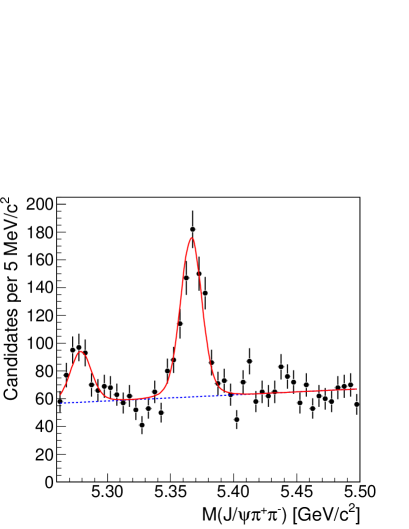
Figure 4: (color online) Projection of the fit of the $B_{s}^{0}\rightarrow J\!/\!\psi f_{0}$ decay mode. The dashed line (blue) shows the contribution from combinatorial background.

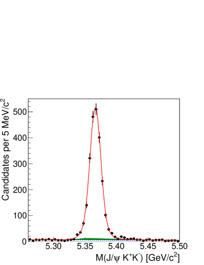
Figure 5: (color online) Projection of the fit of the $B_{s}^{0}\rightarrow J\!/\!\psi\phi$ decay mode. The dashed line (blue) and filled area (green) show the contributions from combinatorial background and $B^{0}\rightarrow J\!/\!\psi K^{*0}$, respectively.

From the fit we find $502\pm 37(\mathrm{stat})\pm 18(\mathrm{syst})$ $B_{s}^{0}\rightarrow J\!/\!\psi f_{0}$ signal events and $2302\pm 49(\mathrm{stat})\pm 49(\mathrm{syst})$ $B_{s}^{0}\rightarrow J\!/\!\psi\phi$ events. The projections of the fits for $B_{s}^{0}\rightarrow J\!/\!\psi f_{0}$ and $B_{s}^{0}\rightarrow J\!/\!\psi\phi$ are shown in Fig. 4 and Fig. 5, respectively.

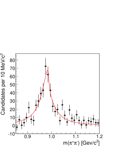
Figure 6: The dipion invariant mass distribution after sideband subtraction with fit projection overlaid. The fit uses a Flatté distribution with all parameters floating.

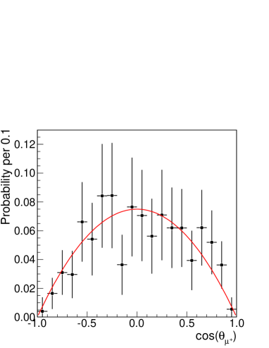
Figure 7: Normalized helicity angle distribution for the positive muon corrected for relative efficiency. The line shows the expectation for a $B_{s}^{0}\rightarrow J\!/\!\psi f_{0}$ decay.

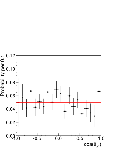
Figure 8: Normalized helicity angle distribution for the positive pion corrected for relative efficiency. The line shows the expectation for a $B_{s}^{0}\rightarrow J\!/\!\psi f_{0}$ decay.

In order to check our interpretation of the signal in the $J\!/\!\psi\pi^{+}\pi^{-}$ distribution being due to the $B_{s}^{0}\rightarrow J\!/\!\psi f_{0}$ decays we show the invariant mass distribution of the pions for $B_{s}^{0}$ signal data in Fig. 6. To obtain the distribution of $B_{s}^{0}$ signal we fit the $J\!/\!\psi\pi^{+}\pi^{-}$ mass distribution in the range 5.26 to 5.45 $\mathrm{GeV}/c^{2}$ for each bin in $\pi^{+}\pi^{-}$ mass and report the $B_{s}^{0}$ signal yield as a function of $\pi^{+}\pi^{-}$ mass. We fit the dipion mass distribution using the Flatté parametrization. The fit probability is 23.4% and the obtained parameters, $m_{0}=989.6\pm 9.9(\mathrm{stat})$ $\mathrm{MeV}/c^{2}$, $g_{\pi}=141\pm 19(\mathrm{stat})$ $\mathrm{MeV}/c^{2}$, and $g_{K}/g_{\pi}=2.3\pm 1.3(\mathrm{stat})$, are in reasonable agreement with the ones measured by the BES collaboration Ablikim:2004wn . In Figs. 7 and 8 we show the positive muon and pion helicity angle distributions, obtained in an analogous way to the invariant mass distribution of pion pairs. Those are corrected for relative efficiencies in the different helicity bins and compared to the theoretical expectation for a $B_{s}^{0}\rightarrow J\!/\!\psi f_{0}$ signal. We use a $\chi^{2}$ test to evaluate the agreement between data and theoretical expectation. For the distribution of $\cos(\theta_{\mu^{+}})$ we obtain $\chi^{2}/\mathrm{ndf}=7.9/20$, which corresponds to 99% probability. Similarly for $\cos(\theta_{\pi^{+}})$ the $\chi^{2}/\mathrm{ndf}$ is $15/20$, giving 78% probability. Since the dipion mass as well as the angular distributions are consistent with expectations, we interpret our signal as coming solely from the $B_{s}^{0}\rightarrow J\!/\!\psi f_{0}$ decays. On the other hand, as we use a dipion mass window from 0.85 to 1.2 $\mathrm{GeV}/c^{2}$, we cannot exclude contributions from other higher mass states to our signal with present statistics.

Finally, we obtain the ratio of branching fractions

$$R_{f_{0}/\phi} = \frac{\mathcal{B}(B_{s}^{0}\rightarrow J\!/\!\psi f_{0})}{\mathcal{B}(B_{s}^{0}\rightarrow J\!/\!\psi\phi)}\frac{\mathcal{B}(f_{0}\rightarrow\pi^{+}\pi^{-})}{\mathcal{B}(\phi\rightarrow K^{+}K^{-})}=$$ (10)

$$0.257\pm 0.020(\mathrm{stat})\pm 0.014(\mathrm{syst}),$$

where corrections for events with an $f_{0}$ or $\phi$ mass outside the ranges selected in this analysis are taken into account.

V Lifetime measurement

In this Section we discuss the details of the lifetime measurement. We describe the maximum likelihood fit, estimate the systematic uncertainties, and present the result of the lifetime measurement.

V.1 Fit description

To extract the $B_{s}^{0}$ lifetime we use a maximum likelihood fit. The fit uses three variables: the invariant mass $m_{i}$, the decay time $t_{i}$, and the decay time uncertainty $\sigma_{ti}$ of each candidate. To exclude $B^{0}\rightarrow J\!/\!\psi\pi^{+}\pi^{-}$ decays we use only candidates with an invariant mass greater than 5.3 $\mathrm{GeV}/c^{2}$ in the fit.

The components in the fit are $B_{s}^{0}$ signal and combinatorial background. The likelihood function has the form

$$\mathcal{L}=\prod_{i=1}^{N} \left[f_{s}\cdot P_{s}(m_{i},t_{i},\sigma_{ti})+\right.$$ (11)

$$\left.(1-f_{s})\cdot P_{cb}(m_{i},t_{i},\sigma_{ti})\right].$$

The parameter $f_{s}$ denotes the fraction of signal $B_{s}^{0}\rightarrow J\!/\!\psi f_{0}$ decays and $P_{s}$ and $P_{cb}$ the probability density function of signal and combinatorial background, respectively. To enhance the signal-to-background ratio in the selected sample, we use only $B_{s}^{0}$ candidates with decay times larger than $0.2$ mm$/c=0.67$ ps. This requirement suppresses background by a factor of 40 and reduces the prompt background component to a negligible level while keeping about two thirds of the signal events.

The $B_{s}^{0}$ signal mass PDF is parametrized as for the branching ratio measurement. The PDF in decay time is parametrized with an exponential function convolved with a Gaussian resolution function. The width of the Gaussian is given by the candidate-specific estimated decay time uncertainty $\sigma_{ti}$ scaled by a common factor $S_{t}$ which accounts for possible discrepancies between estimated and actual resolutions. The scaling factor $S_{t}$ is determined in a fit to data dominated by prompt background, selected by requiring $0<t<0.3$ ps. In the final fit, $S_{t}$ is a free parameter with a Gaussian constraint included as additional factor in the likelihood in Eq. (11). The PDF in decay time uncertainty is parametrized by an empirical function. We use a log-normal distribution with parameters $\mu$, $\theta$, and $\sigma$ defined as

$$\mathcal{D}(\sigma_{ti}|\mu,\theta,\sigma)=\frac{1}{\sqrt{2\pi}\sigma(\sigma_{ti}-\mu)}\cdotp e^{-\frac{(\mathrm{ln}(\sigma_{ti}-\mu)-\theta)^{2}}{2\sigma^{2}}}$$ (12)

for $\sigma_{ti}>\mu$ and zero otherwise. Given the rather small statistics of the $B_{s}^{0}$ signal we derive the parameters using simulated $B_{s}^{0}\rightarrow J\!/\!\psi f_{0}$ events and Gaussian constrain the values in the fit to data. The widths of the Gaussian constraints are chosen to cover possible differences between simulation and data.

The combinatorial background is described by two components, a long-lived part for the background from $b$-hadron decays and a short-lived part for the tail from mis-reconstructed prompt events. The mass PDF is common to both components and parametrized by a linear function. The decay time PDF of each component is described by an exponential convolved with the same resolution function as used for signal. Both decay time uncertainty PDFs are again modeled using log-normal distributions. The parameters of each log normal distribution are independent of the distribution of the $B_{s}^{0}$ signal.

All parameters of the combinatorial background are determined from the fit. The yield, the mass resolution scale factor, and the lifetime of the $B_{s}^{0}$ signal are also left to float freely. The decay time uncertainty parameters of the signal and the resolution scale parameter are Gaussian constrained. Using an ensemble of simulated experiments we verify within 1% that the fit is unbiased and returns proper uncertainties.

V.2 Systematic uncertainties

We investigate several possible sources of systematic uncertainties. These are broadly separable into two classes: the first dealing with the parametrization of the PDFs and the second with possible biases in the selection or reconstruction.

We first investigate our assumption of the mass shape of combinatorial background. We determine the relative change of the $B_{s}^{0}$ lifetime between a fit with a first and a third order polynomial background mass model. For fits in different invariant mass ranges, we find an average difference of 0.010 ps, which we assign as the systematic uncertainty. The systematic uncertainty assigned to the signal mass shape has contributions from the limited knowledge of the mean position and from the assumed shape parametrization. Both effects are evaluated in the same way as for the branching ratio measurement and yield a systematic uncertainty of 0.005 ps. There are two assumptions made for the decay time PDFs; one is the resolution scale factor, $S_{t}$, which is known only with limited precision and the other is the shape of the combinatorial background. The uncertainty of the scale $S_{t}$ is included directly in the statistical uncertainty of the fit as the parameter is allowed to vary within a Gaussian constraint. To quantify the size of the contribution, we repeat the fit with $S_{t}$ fixed to its central value and find the quadratic difference in uncertainty to the original fit to be 0.005 ps. To estimate the effect of the assumed decay time PDF of combinatorial background, we employ an alternative fit method which does not need a decay time parametrization of the background. We split the data into 20 decay time bins and simultaneously fit the invariant mass distributions with independent parameters for the background in each bin. The signal yield per bin is given by the total signal yield times the integral of the signal decay time PDF over the time bin, where the same PDF parametrization as in the default fit is used. The difference in the fit results is taken as a measure of the systematic uncertainty due to the background decay time PDF. To avoid possible statistical fluctuations in this estimate we repeat the comparison for different selection requirements and assign the average difference of 0.021 ps as systematic uncertainty. The third kind of systematic effect addresses the uncertainty of the $\sigma_{t}$ PDFs. The main effect is the distribution for signal derived from simulated events. The uncertainty is already included in the statistical error since the parameters are Gaussian constrained in the fit. The contribution due to modeling of the decay time uncertainty distribution, estimated from a comparison of fit results with fixed and constrained parameters, is 0.015 ps.

For the second class, we verify that our candidate selection does not introduce any significant bias. A bias in the mass distribution could artificially enhance or decrease the amount of signal candidates while a bias in decay time could directly affect the extracted lifetime. We verify on a background-enriched sample selected by requiring $t<0.01$ cm$/c$ that no artificial peak is observed for any neural network output requirement. With a high statistics sample of simulated events we check that the selection does not bias the fitted lifetime. A possible lifetime bias introduced by the trigger has been studied in a previous CDF analysis Aaltonen:2010pj and is negligible in our measurement. Finally the alignment of the tracking detectors is known only with finite precision. Previous measurements found that the uncertainty on the lifetime due to a possible misalignment is 0.007 ps Aaltonen:2010pj .

All the contributions are added in quadrature and yield a total systematic error on the lifetime of 0.03 ps (1.5%). A summary of the systematic uncertainties on the lifetime is provided in Table 2.

Table 2: Summary of assigned systematic uncertainties for the lifetime measurement. The uncertainties in parentheses are included in the statistical uncertainty via Gaussian constraints in the fit.

Source	Uncertainty [ps]
Background mass model	0.010
Signal mass model	0.005
Decay time uncertainty scale	($0.005$)
Background decay time model	0.021
Decay time uncertainty model	(0.015)
SVX alignment	0.007
Total	0.03

V.3 Lifetime result

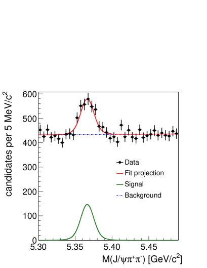
Figure 9: (color online) Invariant mass distribution with fit projection overlaid.

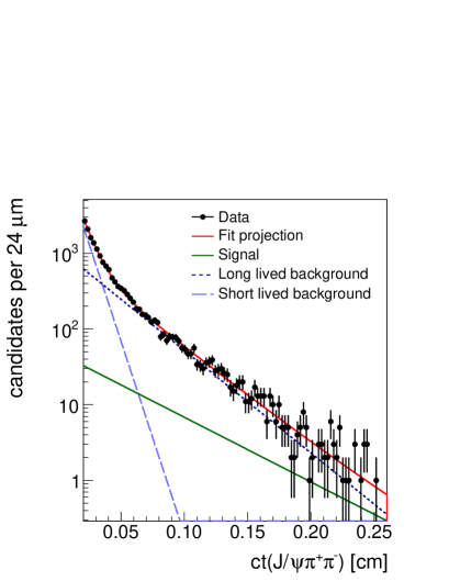
Figure 10: (color online) Decay time distribution with fit projection overlaid.

Figure 11: (color online) Decay time uncertainty distribution with fit projection overlaid.

Performing the likelihood fit to the selected data we extract the $B_{s}^{0}$ lifetime in $B_{s}^{0}\rightarrow J\!/\!\psi f_{0}$ decays

$$\tau(B_{s}^{0}\rightarrow J\!/\!\psi f_{0})=1.70_{-0.11}^{+0.12}(\mathrm{stat})\pm 0.03(\mathrm{syst})\,\mathrm{ps}.$$ (13)

In Figs. 9 to 11 we show the data together with the projection of the fit.

VI Conclusions

We confirm the observation of the $B_{s}^{0}\rightarrow J\!/\!\psi f_{0}(980)$ decay from the LHCb Aaij:2011fx and Belle Li:2011pg experiments. The observed signal is the world’s largest and we perform the most precise measurement of the ratio of branching fractions $R_{f_{0}/\phi}$ between $B_{s}^{0}\rightarrow J\!/\!\psi f_{0}$ and $B_{s}^{0}\rightarrow J\!/\!\psi\phi(980)$ decays:

$$R_{f_{0}/\phi} = \frac{\mathcal{B}(B_{s}^{0}\rightarrow J\!/\!\psi f_{0}(980))}{\mathcal{B}(B_{s}^{0}\rightarrow J\!/\!\psi\phi)}\frac{\mathcal{B}(f_{0}(980)\rightarrow\pi^{+}\pi^{-})}{\mathcal{B}(\phi\rightarrow K^{+}K^{-})}=$$ (14)

$$0.257\pm 0.020(\mathrm{stat})\pm 0.014(\mathrm{syst}).$$

In this result we assume that the observed signal is solely due to the decay $B_{s}^{0}\rightarrow J\!/\!\psi f_{0}(980)$ and correct for the acceptance of the invariant mass selection of the pion pair. Using the world average $B_{s}^{0}\rightarrow J\!/\!\psi\phi$ branching fraction Nakamura:2010zzi $R_{f_{0}/\phi}$ can be converted into the product of branching fractions of

$$\mathcal{B}(B_{s}^{0}\rightarrow J\!/\!\psi f_{0}(980))\mathcal{B}(f_{0}(980)\rightarrow\pi^{+}\pi^{-})=$$

$$(1.63\pm 0.12\pm 0.09\pm 0.50)\times 10^{-4},$$ (15)

where the first uncertainty is statistical, the second is systematic, and the third one is due to the uncertainty on the $B_{s}^{0}\rightarrow J\!/\!\psi\phi$ and $\phi\rightarrow K^{+}K^{-}$ branching fractions. The measurement presented here agrees well with the previous measurements of this quantity and with theoretical predictions.

Moreover, our sample allows us to measure the $B_{s}^{0}$ lifetime in the $B_{s}^{0}\rightarrow J\!/\!\psi f_{0}(980)$ decay mode:

$$\tau(B_{s}^{0}\rightarrow J\!/\!\psi f_{0}(980))=1.70_{-0.11}^{+0.12}(\mathrm{stat})\pm 0.03(\mathrm{syst})\,\mathrm{ps}.$$ (16)

This is the first measurement of the $B_{s}^{0}$ lifetime in a decay to a pure CP eigenstate. In the context of the standard model the lifetime measured in this decay mode to a CP-odd final state can be interpreted as the lifetime of the heavy $B_{s}^{0}$ eigenstate. The measured value agrees well both with the standard model expectation as well as with other experimental determinations.

While the precision of the lifetime measurement is still limited by statistics, it provides an important cross-check on the result determined in $B_{s}^{0}\rightarrow J\!/\!\psi\phi$ decays, which relies on an angular separation of two CP eigenstates. Furthermore, the measured lifetime can be used as an external constraint in the $B_{s}^{0}\rightarrow J\!/\!\psi\phi$ analysis to improve the determination of the CP-violating phase in the $B_{s}^{0}\rightarrow J\!/\!\psi\phi$ decay. The lifetime measurement in $B_{s}^{0}\rightarrow J\!/\!\psi f_{0}(980)$ decays is also the next step towards a tagged time dependent CP-violation measurement, which can provide an independent constraint on the CP violation in $B_{s}^{0}$ mixing.

We thank the Fermilab staff and the technical staffs of the participating institutions for their vital contributions. This work was supported by the U.S. Department of Energy and National Science Foundation; the Italian Istituto Nazionale di Fisica Nucleare; the Ministry of Education, Culture, Sports, Science and Technology of Japan; the Natural Sciences and Engineering Research Council of Canada; the National Science Council of the Republic of China; the Swiss National Science Foundation; the A.P. Sloan Foundation; the Bundesministerium für Bildung und Forschung, Germany; the Korean World Class University Program, the National Research Foundation of Korea; the Science and Technology Facilities Council and the Royal Society, UK; the Institut National de Physique Nucleaire et Physique des Particules/CNRS; the Russian Foundation for Basic Research; the Ministerio de Ciencia e Innovación, and Programa Consolider-Ingenio 2010, Spain; the Slovak R&D Agency; and the Academy of Finland.

References

- (1) A review of mixing can, for example, be found in C. Gay, Annu. Rev. Nucl. Part. Sci. 50, 577 (2000).
- (2) A. Lenz and U. Nierste, J. High Energy Phys. 06, 072 (2007).
- (3) U. Nierste and A. Lenz, arXiv:hep-ph/1102.4274.
- (4) I. Dunietz, R. Fleischer, and U. Nierste, Phys. Rev. D 63, 114015 (2001).
- (5) A. S. Dighe, I. Dunietz, H. J. Lipkin, and J. L. Rosner, Phys. Lett. B 369, 144 (1996).
- (6) S. Stone and L. Zhang, arXiv:hep-ex/0909.5442.
- (7) T. Aaltonen et al. (CDF Collaboration), Phys. Rev. Lett. 100, 161802 (2008).
- (8) V. M. Abazov et al. (D0 Collaboration), Phys. Rev. Lett. 101, 241801 (2008).
- (9) S. Stone and L. Zhang, Phys. Rev. D 79, 074024 (2009).
- (10) S. Stone, arXiv:hep-ph/1009.4939.
- (11) F. Azfar et al., J. High Energy Phys. 1011, 158 (2010).
- (12) T. Aaltonen et al. (CDF Collaboration), CDF Public Note 10206, 2010 (unpublished).
- (13) T. Aaltonen et al. (CDF Collaboration), Phys. Rev. D83, 052012 (2011).
- (14) K. Nakamura et al. (Particle Data Group), J. Phys. G 37, 075021 (2010).
- (15) D. Asner et al. (Heavy Flavor Averaging Group), arXiv:hep-ex/1010.1589.
- (16) K. Ecklund et al. (CLEO Collaboration), Phys. Rev. D 80, 052009 (2009).
- (17) O. Leitner, J.-P. Dedonder, B. Loiseau, and B. El-Bennich, Phys. Rev. D 82, 076006 (2010).
- (18) P. Colangelo, F. De Fazio, and W. Wang, Phys. Rev. D 81, 074001 (2010).
- (19) P. Colangelo, F. De Fazio, and W. Wang, arXiv:hep-ph/1009.4612.
- (20) R. Louvot, arXiv:hep-ex/1009.2605.
- (21) R. Aaij et al. (LHCb Collaboration), Phys. Lett. B 698, 115 (2011).
- (22) J. Li et al. (Belle Collaboration), Phys. Rev. Lett. 106, 121802 (2011).
- (23) R. Louvot, arXiv:hep-ex/0905.4345.
- (24) D0 Collaboration, Conference Note 6152
- (25) D. E. Acosta et al. (CDF Collaboration), Phys. Rev. D 71, 032001 (2005).
- (26) C. S. Hill, Nucl. Instrum. Methods A 530, 1 (2004).
- (27) A. A. Affolder et al., Nucl. Instrum. Methods A 526, 249 (2004).
- (28) L. Balka et al., Nucl. Instrum. Methods A 267, 272 (1988).
- (29) S. Bertolucci et al., Nucl. Instrum. Methods A 267, 301 (1988).
- (30) M. G. Albrow et al., Nucl. Instrum. Methods A 480, 524 (2002).
- (31) G. Apollinari, K. A. Goulianos, P. Melese, and M. Lindgren, Nucl. Instrum. Methods A 412, 515 (1998).
- (32) G. Ascoli et al., Nucl. Instrum. Methods A 268, 33 (1998).
- (33) E. J. Thomson et al., IEEE Trans. Nucl. Sci., 49, 1063 (2002).
- (34) M. Feindt and U. Kerzel, Nucl. Instrum. Methods A 559, 190 (2006).
- (35) M. Feindt, arXiv:physics/0402093.
- (36) D. Lange, Nucl. Instrum. Methods A 462, 152 (2001).
- (37) R. Brun, R. Hagelberg, M. Hansroul, and J. Lassalle, CERN-DD-78-2-REV, 1978 (unpublished).
- (38) E. Gerchtein and M. Paulini, arXiv:physics/0306031.
- (39) G. Giurgiu, Ph.D. thesis, Carnegie Mellon University, FERMILAB-THESIS-2005-41, 2005.
- (40) G. Punzi, arXiv:physics/0308063.
- (41) F. Abe et al. (CDF Collaboration), Phys. Rev. D 54, 6596 (1996).
- (42) M. Gronau and J. L. Rosner, Phys. Lett. B 669, 321 (2008).
- (43) S. M. Flatté, Phys. Lett. B 63, 224 (1976).
- (44) M. Ablikim et al. (BES Collaboration), Phys. Lett. B 607, 243 (2005).
- (45) T. Aaltonen et al. (CDF Collaboration), Phys. Rev. Lett. 106, 121804 (2011).