The Formation and Coarsening of the Concertina Pattern

Abstract

The concertina is a magnetization pattern in elongated thin-film elements of a soft material. It is a ubiquitous domain pattern that occurs in the process of magnetization reversal in direction of the long axis of the small element.

Van den Berg argued that this pattern grows out of the flux closure domains as the external field is reduced. Based on experimental observations and theory, we argue that in sufficiently elongated thin-film elements, the concertina pattern rather bifurcates from an oscillatory buckling mode.

Using a reduced model derived by asymptotic analysis and investigated by numerical simulation, we quantitatively predict the average period of the concertina pattern and qualitatively predict its hysteresis. In particular, we argue that the experimentally observed coarsening of the concertina pattern is due to secondary bifurcations related to an Eckhaus instability.

We also link the concertina pattern to the magnetization ripple and discuss the effect of a weak (crystalline or induced) anisotropy.

I Introduction

To our knowledge, the term concertina was introduced by van den Berg et. al. in [20, p.880]. In that paper he explains the formation of this domain pattern in Permalloy thin-film elements that are fairly thick (thickness $t=350$nm), with a rectangular cross section (width $\ell=15\upmu$m) that is not too elongated (length $60\upmu$m). After near-saturation along the long axis, a concertina pattern grows out of the flux closure domains at the short edges of the cross section during subsequent reduction of the external field $H_{\text{ext}}$, until the pattern eventually invades the entire sample, see Figure 1 on the right. Our experimental observations suggest that in very elongated samples (length $2$nm, thickness $10$ to $150$nm, width $10$ to $100\upmu$m) a bifurcation is at the origin of the concertina. As a consequence, the pattern forms simultaneously all over the sample. We will report on van den Berg’s explanation in more detail after introducing the micromagnetic model.

[1]

Figure 1: Concertina in a very elongated (length $2$ mm) sample of width $50\,\upmu$m and thickness $50$ nm (left) and in a sample of width $35\,\upmu$m, thickness $40$ nm and moderate length $110\,\upmu$m (right). The left image shows only the center of the stripe which is less than $10$ percent of the whole sample. As indicated by the blue arrows, the gray scales encode the transversal component of the magnetization in the domains.

Figure 2: Formation of the concertina pattern in the experiment: The pictures show a section near the center of the elongated thin-film element. The unstable mode grows into a domain-wall pattern which coarsens several times. The two upper series show a sample of $30$nm thickness of low anisotropy. The two lower series show a sample of $30$nm thickness of higher anisotropy. The width is $30\upmu$m and $50\upmu$m, respectively.

I.1 The micromagnetic energy

The variation of the applied magnetic field in the experiments is on a very slow time-scale so that the magnetization always relaxes to equilibrium. Hence our theoretical analysis is based on the micromagnetic (free) energy, which we introduce now. The magnetization of a ferromagnetic sample occupying some domain $\Omega$ is described by a vector field $m=(m_{1},m_{2},m_{3})$. The micromagnetic energy $E(m)$ is given by

$$\begin{split}E(m)=\,&d^{2}\int_{\Omega}|\nabla m|^{2}\,\operatorname{d}\!x+\int_{\text{all space}}|H_{\text{stray}}|^{2}\,\operatorname{d}\!x\\ &{}-Q\int_{\Omega}(m\cdot e)^{2}\,\operatorname{d}\!x-2\,\int_{\Omega}H_{\text{ext}}\cdot m\,\operatorname{d}\!x.\end{split}$$ (1)

The energy (1) is already partially, i.e., except for lengths, non-dimensionalized. In particular the magnetization has length one. Outside of the sample, it vanishes identically:

$$\begin{split}&|m|^{2}=1\quad\text{ in the sample }\Omega,\\ &m=0\quad\text{ outside of the sample }\Omega.\end{split}$$ (2)

Let us now briefly introduce and discuss the different energy contributions:

The first contribution in (1) is the so called exchange energy. (The gradient acts component wise, i.e., $|\nabla m|^{2}=\sum_{i=1}^{3}\sum_{j=1}^{3}(\partial_{i}m_{j})^{2}$.) This term favors a uniform magnetization. The material parameter $d$ is called the exchange length and measures the relative strength of exchange with respect to stray-field energy, see below. The exchange length is typically of the order of a few nano-meters.

The second contribution in (1) is the stray-field energy. The static Maxwell equations state that the magnetization $m$ generates a stray field $H_{\text{stray}}$ that is described by

$$\begin{split}&\nabla\times H_{\text{stray}}=0,\\ &\nabla\cdot(H_{\text{stray}}+m)=0,\end{split}$$ (3)

where both equations hold in the whole space and $B=H_{\text{stray}}+m$ is the magnetic induction. Hence the stray field is generated by the divergence of the magnetization. Since the magnetization is discontinuous at the boundary of the sample $\partial\Omega$, cf. (2), the second equation in (3) has to be understood in the following sense:

$$\begin{split}\nabla\cdot H_{\text{stray}}&=\begin{cases}-\nabla\cdot m&\text{ in the sample }\Omega\\ 0&\text{ outside of the sample }\Omega,\end{cases}\\ [H_{\text{stray}}\cdot\nu]&=m\cdot\nu\text{ on the boundary }\partial\Omega,\end{split}$$ (4)

where $\nu$ denotes the normal to the boundary of the sample, and $[H_{\text{stray}}\cdot\nu]$ denotes the jump that $H_{\text{stray}}\cdot\nu$ experiences across the boundary $\partial\Omega$. Hence we distinguish two different types of sources of the stray field – in analogy to electrostatics one commonly speaks of charges – namely

$$\text{magnetic volume charges }\quad\nabla \cdot m\quad\text{ in }\quad\Omega\quad\text{ and }$$

$$\text{magnetic surface charges }\quad\nu \cdot m\quad\text{ on }\quad\partial\Omega.$$

Later on we will also use the following equivalent distributional formulation of (4), which is obtained by testing with smooth functions $\zeta$ vanishing at infinity, namely

$$\int_{\text{all space}}H_{\text{stray}}\cdot\nabla\zeta\,\operatorname{d}\!x=-\int_{\Omega}m\cdot\nabla\zeta\,\operatorname{d}\!x.$$ (5)

The third contribution in (1) models a uniaxial anisotropy, i.e., the preference of an easy axis $e=(e_{1},e_{2},e_{3})$ in a material. The material parameter $Q>0$ is called the quality factor. It measures the relative strength of anisotropy with respect to stray-field energy. A uniaxial anisotropy can for example come in form of crystalline or induced anisotropy. Notice that the polycrystalline anisotropy in a material like Permalloy can be described as a position-dependent easy axis $e(x)$.

The last contribution in (1) is called Zeeman energy. This term models the interaction and favors the alignment of the magnetization with an external magnetic field $H_{\text{ext}}$.

The specific material parameters of our samples are discussed in Section I.4.

I.2 Van den Berg’s explanation of the concertina

We now return to van den Berg’s paper [20]. Combining the explanation of the formation of the concertina pattern therein with the insight from [3, 7], we can give the following updated version of the explanation presented in [20, Sections A & B]: It is a theory on the two-dimensional mesoscopic magnetization pattern; by two-dimensional, we understand that the magnetization is in-plane,i.e., $m_{3}=0$, and independent of the thickness direction, i.e., $m=m(x_{1},x_{2})$; by mesoscopic, we understand that the walls are replaced by sharp discontinuity curves that are charge-free in the sense that the normal component of the magnetization does not jump; moreover, the magnetization is tangential to the lateral edges of the sample so that there are no surface charges. In sufficiently large thin-film elements and for sufficiently low external fields, [3] now postulate that the two-dimensional mesoscopic magnetization pattern arranges itself in such a way that the corresponding continuous magnetic charge density $\sigma=-(\partial_{1}m_{1}+\partial_{2}m_{2})$ generates a stray field $H_{stray}$ that expels the external field $H_{\text{ext}}$ from inside of the sample (like in electrostatics).

In [8], see [7] for an efficient account, it is shown that in the regime of sufficiently large thin-film elements (i.e., $t\ll\ell$ and $\ell t\gg d^{2}\log\frac{\ell}{t}$ with comparable lateral dimensions of the order $\sim\ell$), this principle extends to moderately large fields (of the order $\sim\frac{t}{\ell}$): In this case, the stray field $H_{\text{stray}}$ in general can no longer expel the external field $H_{\text{ext}}$ everywhere in the sample, since the (total) charge density $\sigma=-(\partial_{1}m_{1}+\partial_{2}m_{2})$ is limited by $m_{1}^{2}+m_{2}^{2}=1$. The charge density $\sigma$ is uniquely determined by a convex variational problem only involving the stray-field energy and the Zeeman energy. At least some aspects of the mesoscopic two-dimensional magnetization pattern $(m_{1},m_{2})$ can be recovered from $\sigma$: The characteristics of $(m_{1},m_{2})$, i.e., the curves along which $(m_{1},m_{2})$ is normal (called “trajectories in [20]), have curvature given by $\sigma$. However, due to the potential discontinuity curves of the mesoscopic magnetization $(m_{1},m_{2})$, this seemingly rigid condition does not suffice to determine $(m_{1},m_{2})$ – even the fact that the discontinuity curves are charge-free is still not enough. Notice that it is easy to construct a particular solution $(m_{1},m_{2})$ for any charge density $\sigma$ via the maximal solution of a modified eikonal equation [7, p.2987]). On the other hand, in the region where the external field has penetrated, the magnetization $(m_{1},m_{2})$ is uniquely determined, cf. [7, p.2987], and has no discontinuities, cf. [20, p.883].

Van den Berg gives a recipe how to construct a solution that corresponds to the experimental observation of a concertina pattern growing out of the flux closure pattern: For sufficiently large external fields ($H_{\text{ext}}=(h_{\text{ext}},0,0)$, $h_{\text{ext}}\gg\frac{t}{\ell}$), $H_{\text{ext}}+H_{stray}$ does not vanish in the sample besides in the vicinity of the two distant edges; as a consequence walls only occur in the two flux closure pattern there. As the external field is reduced, the penetrated region shrinks as the walls invade the sample. Each of the two flux closure pattern has a “doublet”, that is, a point on one of the long edges where two wall segments intersect. Note that the doublets were created as the central $180^{\circ}$-wall of the initial Landau state moved towards the edge where it broke up due to the application of a large external field at the very beginning. The inner, i.e., most distant to the short edges, ones of the doublet walls fade out in the middle (with respect to the long edges) of the cross section. Van den Berg postulates that the position of the doublets does not change as the external field decreases further. As a consequence, each of the two inner walls grows – necessarily in direction of the characteristic – till is hits the opposite edge. There it must generate a “triplet” (a point on the edge where three walls meet); the middle wall must coincide with the previous one originating in the doublet. Again, as the external field is further reduced, the position of each triplet is supposed to be fixed, the inner of the three walls grows towards the opposite edge.

Figure 3: The creation of a triplet out of the initial doublet as described and sketched by van den Berg in [20]

This process repeats itself till the two half-concertina structures growing from the short edges are linked in the middle (with respect to the short edges) of the cross section. For very elongated samples of length $L\gg\ell$, the linking is expected at a field strength of order $h_{\text{ext}}\sim t\ell L^{-2}\ln t\ell^{-1}$ and thus differs from the field at the beginning of the growth process by a factor $\ell^{2}L^{-2}$ (up to a logarithm). Speaking in mathematical terms, van den Berg postulates that the positions of doublets and triplets remain fixed as the field is decreased and appeals to continuity, i.e., the pattern should depend continuously on the value of the external field, to overcome the non-uniqueness of $(m_{1},m_{2})$ mentioned in the previous paragraph.

I.3 Van den Berg’s vs. our explanation

Our explanation for the formation of the concertina pattern is very different from the one of van den Berg. Instead of a successive outgrowth (along the sample) of the closure domains, we explain the concertina as a simultaneous outgrowth (along the sample) of an unstable mode, best captured in very elongated thin-film elements. Indeed, our experiments were performed on thin-film elements of thicknesses $t$ in the range of $10$nm to $150$nm, widths $\ell$ in the range of $10\upmu$m to $100\upmu$m, but lengths in the range of $2$mm. We recorded the pattern at three different sections, equidistant and equidistant to the short edges of the cross section, and observed qualitatively the same pattern at the same values of the external field.

Not surprisingly, our theoretical predictions are quite different from those in [20] – already in terms of scaling. Van den Berg’s explanation entails two different scales of the external field

• $h_{\text{ext}}^{\text{begin}}\sim\frac{t}{\ell}$ for the beginning of the build-up process and

• $h_{\text{ext}}^{\text{end}}\sim t\ell L^{-2}\ln t\ell^{-1}$ for the completion when the external field is totally expelled from the sample

whereas in our case there is one critical field $h_{\text{ext}}^{*}$ at which the simultaneous formation of the concertina along the sample – independently of the specific position – due to an interior instability begins. This critical field is given by $h_{\text{ext}}^{*}\sim-d^{2/3}\ell^{-4/3}t^{2/3}$, see Regime III in Subsection I.6, for isotropic samples – thus the instability would only occur after the field is reversed and thus when the van den Berg concertina has already invaded the sample. However, as we discuss later, the critical field is shifted in case of a transversal anisotropy $h_{\text{ext}}^{*}\leadsto h_{\text{ext}}^{*}+Q$. It turns out that even for relatively weak transversal anisotropy the formation thus starts before the field is reversed, see Section VI, a). For very elongated samples, i.e., $L\gg\ell$, we have that $h_{\text{ext}}^{\text{begin}}\gg h_{\text{ext}}^{\text{end}}$ and $h_{\text{ext}}^{\text{end}}=0$ for the limit case of an infinitely extended sample. The strength of the anisotropy and the geometry of the majority of the samples that we investigated is such that $h_{\text{ext}}^{\text{begin}}\gg h_{\text{ext}}^{*}\gg h_{\text{ext}}^{\text{end}}$. We thus expect the following scenario in very elongated samples: At $h_{\text{ext}}^{\text{begin}}$ the van den Berg build-up process starts at the tips of the sample. As the field is reduced, the concertina grows slowly into the sample from the tips. Meanwhile, as $h_{\text{ext}}^{*}$ is attained our instability occurs all over the sample – sufficiently far away from the tips and way before the van den Berg linking could take place in the center of the sample, see Table 1.

	$h_{\text{ext}}^{\text{begin}}$	$h_{\text{ext}}^{*}$	$h_{\text{ext}}^{\text{end}}$
Weak anisotropy
($Q=1.3\times 10^{-4}$)
$\ell=30\upmu$m	$1\times 10^{-3}$	$-4.0\times 10^{-5}$	$1.6\times 10^{-6}$
$\ell=50\upmu$m	$6\times 10^{-4}$	$4.2\times 10^{-5}$	$2.8\times 10^{-6}$
Stronger anisotropy
($Q=5.0\times 10^{-4}$)
$\ell=30\upmu$m	$1\times 10^{-3}$	$3.4\times 10^{-4}$	$1.6\times 10^{-6}$
$\ell=50\upmu$m	$6\times 10^{-4}$	$4.2\times 10^{-4}$	$2.8\times 10^{-6}$

Table 1: Comparison of the characteristic fields in van den Berg’s theory of the concertina and the critical field in our instability for the samples shown in Figure 2 (thickness $t=30$nm, length $L=2$mm. Apart from the sample of weak anisotropy and small width, the characteristic fields appear in the expected order.

Whereas in [20] the appropriate scale for the concertina width $w$ is given by $\ell$ – in particular independent on the thickness $t$ – it is given by and $d^{2/3}\ell^{2/3}t^{-1/3}$ in our case, in qualitative accordance with our experimental observations illustrated in Figure 4.

Figure 4: Concertina in Permalloy samples of width $\ell=100\upmu$m and thickness $t=30$nm (left), $t=80$nm (center), and $t=300$nm (right). The width average period of the pattern is a decreasing function of the thickness $t$.

I.4 Experimental setup and samples

In the experiments, we investigated magnetic films of nano-crystalline Permalloy (Ni₈₁Fe₁₉) and amorphous Co₆₀Fe₂₀B₂₀ of various thicknesses and induced magnetic anisotropy values. The films were deposited by magnetron sputtering under ultra-high vacuum conditions. In order to control the grain growth of the polycrystalline films, a Ta seed ($5$ nm) layer was used for the Ni₈₁Fe₁₉ deposition. In all cases a magnetic in-plane saturation field was applied during film deposition to control strength and direction of the induced anisotropy. Using different magnetic field histories, films of different effective induced anisotropy were obtained.

• A first set of samples was deposited in the presence of a homogeneous, static magnetic field. This results in a maximal and also well-aligned induced uniaxial anisotropy. A series of Permalloy and CoFeB samples was obtained by this method.

• In a second set of samples the induced anisotropy was strongly reduced. In order to ensure this, the films were deposited in a magnetic field of alternating orthogonal alignment. The field direction was changed after approximately every $5$nm of film growth. The superposition of the so-obtained orthogonal anisotropy axes results in a strongly reduced induced anisotropy.

The relevant material parameters – for the comparison of the experimental observations to the theoretical predictions – are the following:

• Exchange length $d$: Permalloy $5$nm, CoFeB $3$nm.

• For both materials the saturation polarization is $J_{s}\approx 1$T and the stray-field energy density is given by $K_{d}\approx 4\times 10^{5}$ J/m³.

• The uniaxial anisotropy coefficient is $K_{u}^{\text{Permalloy}}\approx 200$ J/m³ for the high-anisotropy Permalloy and $K_{u}^{\text{CoFeB}}\approx 600$ J/m³ for CoFeB, respectively. For the low-anisotropy Permalloy films we have $K_{u}^{\text{Permalloy}}\approx 50$ J/m³.

• Quality factor $Q=K_{u}/K_{d}$: High and low-anisotropy Permalloy $0.5\times 10^{-3}$ and $0.125\times 10^{-3}$, respectively, and CoFeB $1.5\times 10^{-3}$.

• The average size of the individual grains of Permalloy is $\ell_{\text{grain}}\approx 12$ to $15$nm. It is assumed that up to a film thickness of about $30$nm, the grains display a column-like shape.

• The film thicknesses range from $10$ to $150$nm, the film widths from $10$ to $100\upmu$m.

After film deposition, elongated stripes of various widths and a length of $2000\upmu$m were patterned by photolithography and subsequent ion beam etching. The stripes were aligned, both, parallel and orthogonal to the induced anisotropy direction.

The observation of domains and magnetization processes was carried out in a digitally enhanced Kerr microscope, [15]. The longitudinal Kerr effect was applied with its magneto-optical sensitivity direction transversal to the stripe axis. The dominant wavelength of the observed concertina patterns was computed by Fast Fourier Transform. The result of the computation is in agreement with the average wavelength determined by manually counting the folds in the images, as soon as the concertina becomes discernible to the eye during field reduction. The typical strength of the magnetic field, which is applied for the saturation at the very beginning, is of the order of some mT.

I.5 Nucleation

We are interested in the magnetization pattern in elongated thin-film elements of width $\ell$ (in $x_{2}$-direction) and thickness $t\ll\ell$ (in $x_{3}$-direction) that forms under the variation of an external field aligned with the long axis (the $x_{1}$-axis), that is, of the form $H_{\text{ext}}=(-h_{\text{ext}},0,0)$. (To simplify the notations, the minus is introduced which entails a positive critical field, see below.) As indicated above, we observe no influence of the sample’s short edges on the formation of the concertina away from the short edges. Since it greatly simplifies the theoretical treatment, we therefore henceforth will assume that the sample is infinite in $x_{1}$-direction (and occasionally, for instance in the numerical treatment, impose a large, but artificial period in that direction). One consequence of that assumption is that the uniform magnetization $m^{*}=(1,0,0)$ is a stationary point of the energy functional – that is, satisfies the corresponding Euler-Lagrange equations that express a torque balance at every point of the sample – for all values $h_{\text{ext}}$ of the external field $H_{\text{ext}}$ of the form above.

Figure 5: The idealized geometry of the sample. The homogeneous external field $H_{\text{ext}}$ is parallel to the long axis of the sample.

The experiments suggest that as the strength of the field is reduced starting from saturation, i.e., $h_{\text{ext}}<0$, and finally reversed, a bifurcation at some critical value $h_{\text{ext}}^{*}>0$ of the external field $H_{\text{ext}}=(-h_{\text{ext}},0,0)$ is at the origin of the concertina pattern, see Figure 2 and Figure 40. Due to the unit-length constraint (2), infinitesimal variations of $m^{*}$ are of the form $\delta m=(0,\delta m_{2},\delta m_{3})$. Since the uniform magnetization only generates Zeeman energy, the linearization of the energy in $m^{*}$ – neglecting anisotropy – is given by the exchange energy and the stray-field energy of the infinitesimal variation, that is, $d^{2}\int_{\Omega}|\nabla\delta m|^{2}\operatorname{d}\!x+\int_{\text{all space}}|H_{\text{stray}}(\delta m)|^{2}\operatorname{d}\!x$, augmented by the linearization of the Zeeman energy. The latter is due to the constraint (2) given by $-h_{\text{ext}}\int_{\Omega}(\delta m_{2}^{2}+\delta m_{3}^{2})\d{x}$ which is a consequence of the expansion $m_{1}=(1-\delta m_{2}^{2}-\delta m_{3}^{2})^{1/2}\approx 1-\frac{1}{2}(\delta m_{2}^{2}+\delta m_{3}^{2})$.

I.6 Unstable modes

We start with the linear stability analysis of the uniform magnetization by discussing potentially unstable modes on the level of the linearization of the energy. We argue at which value of the external field $h_{\text{ext}}$ each of the modes becomes unstable. At this so-called critical field the infinitesimal release of Zeeman energy becomes larger than the infinitesimal contributions due to exchange and stray-field energy. We neglect uniaxial anisotropy (i.e., we set $Q=0$) for the moment, since on the level of this infinitesimal discussion, a longitudinal or transversal anisotropy just leads to a shift of the critical field $h_{\text{ext}}^{*}\leadsto h_{\text{ext}}^{*}+Q$, see Section VI. Since the shift entails that the sign of the critical field can change, we note in that context that if we speak about reducing the strength of the external field we usually mean that the critical field is approached from saturation ($h_{\text{ext}}=-\infty$) if not stated differently. Similarly we say that the external field is increased after the critical field is passed. In this sense, the critical field is interpreted as the zero point on the scale of the external field, cf. Figure 6.

Figure 6: The scale of the external field $h_{\text{ext}}$.

I) The first mode we discuss is a coherent rotation, i.e., $\delta m=(0,\delta m_{2},\delta m_{3})$ is constant in space. Such a mode releases Zeeman energy per length in $x_{1}$-direction of the infinitesimal amount $h_{\text{ext}}\ell t\delta A^{2}$, where $\delta A=(\delta m_{2}^{2}+\delta m_{3}^{2})^{1/2}$ is the infinitesimal amplitude of the coherent rotation. A coherent rotation necessarily generates surface charges. Since the top and bottom surfaces have larger area than the two lateral surfaces, an in-plane rotation ($\delta m_{3}\equiv 0)$ is favored, cf. Figure 7. This mode generates surface charges of infinitesimal density $\pm\delta A$. Over distances $\ell$ much larger than $t$, these surface charges act like two oppositely charged wires at distance $\ell$ of line density $t\delta A$ – also in the following if not mentioned otherwise always infinitesimally and per length in $x_{1}$-direction. Hence the mode generates an infinitesimal stray field of order $\sim t^{2}(\ln{\ell}{t}^{-1})\delta A^{2}$. Therefore, this mode becomes unstable when $h_{\text{ext}}\sim{t}\ell^{-1}(\ln\ell{t}^{-1})$.

Figure 7: Coherent rotation and generated surface charges.

II) The second mode we consider is buckling, cf. Figure 8. The magnetization avoids the lateral surface charges by just laterally buckling in the middle of the cross section, i.e., $\delta m=(0,\delta A\sin(\pi\frac{x_{2}}{\ell}),0)$. However, since $\nabla\cdot\delta m=\pi\ell^{-1}\delta A\cos(\pi\frac{x_{2}}{\ell})$, the surface charges of the coherent rotation turn into volume charges. At distances much larger than $t$ from the cross section, these volume charges act like surface charges of amplitude $\sim\ell^{-1}t\delta A$. Since these surface charges change sign over a distance $\ell$, they generate a stray field which extends a distance $\sim\ell$ away from the cross section, and which is of the magnitude $\sim\ell^{-1}t\delta A$. Hence this mode generates a stray field energy $\sim t^{2}\delta A^{2}$, which is only smaller by a logarithm than in case of the previous mode of coherent rotation. Moreover, since $|\nabla\delta m|^{2}=\pi^{2}\ell^{-2}\delta A^{2}\cos^{2}(\pi\frac{x_{2}}{\ell})$, the mode generates exchange energy $\sim d^{2}\ell^{-1}t\delta A^{2}$. Since the release of Zeeman energy scales as $\sim h_{\text{ext}}\ell t\delta A^{2}$ as in case of the first mode above, this mode becomes unstable at $h_{\text{ext}}\sim{d^{2}}{\ell}^{-2}$ in the regime $t\ll{d^{2}}\ell^{-1}$ and at $h_{\text{ext}}\sim{t\ell}d^{-2}$ in the regime $t\gg{d^{2}}\ell^{-1}$.

Figure 8: Buckling mode and generated volume charges and stray field – for reasons of a clear presentation only drawn in the region above the sample.

III) The third mode we discuss is oscillatory buckling, cf. Figure 9. This mode reduces the stray-field energy through a modulation of the lateral buckling in $x_{1}$-direction, i.e., $\delta m=(0,\delta A\sin(\pi\frac{x_{2}}{\ell})\sin(2\pi\frac{x_{1}}{w}),0)$ with a wavelength $w$ that satisfies $t\ll w\ll\ell$. Since $w\gg t$, the volume charges generated by this mode act like surface charges of amplitude $\sim\ell^{-1}t\delta A$ over distances much larger than $t$ from the cross section. However, these surface charges change sign over a distance $w\ll\ell$, so that the generated stray field only extends over a distance $\sim w$ away from the cross section. Hence this mode generates a stray-field energy $\sim\ell^{-1}t^{2}w\delta A^{2}$, which is substantially less than the stray-field energy of the two prior modes for $w\ll\ell$. However, since $w\ll\ell$, the exchange energy is now dominated by the oscillation in $x_{1}$-direction, which leads to an infinitesimal exchange energy $\sim d^{2}\ell w^{-2}t\delta A^{2}$. Hence the wavelength $w$ which leads to the minimal infinitesimal total stray-field energy and exchange energy of order $\sim d^{2/3}\ell^{-1/3}t^{5/3}\delta A^{2}$ is given by $w^{*}\sim d^{2/3}\ell^{2/3}t^{-1/3}$. This is consistent with our assumption $t\ll w\ll\ell$ provided $d^{2}\ell^{-1}\ll t\ll(d\ell)^{1/2}$. The oscillatory buckling mode becomes unstable at a field strength of order $h_{\text{ext}}\sim d^{2/3}\ell^{-4/3}t^{2/3}$.

Figure 9: Oscillatory buckling mode and generated surface charges and stray field – for reasons of a clear presentation only drawn in the region above the sample.

IV) The fourth mode we consider is curling. This mode avoids charges altogether by an $x_{3}$-dependent magnetization, i.e., $\delta m=(0,\delta A\sin(\pi\frac{x_{2}}{\ell})\cos(\pi\frac{x_{3}}{t}),\delta A\ell^{-1}t\cos(\pi\frac{x_{2}}{\ell})\sin(\pi\frac{x_{3}}{t}))$. The exchange energy in this case is dominated by the gradient in $x_{3}$-direction which scales as $\sim d^{2}\ell t^{-1}\delta A^{2}$. Hence the curling mode becomes unstable at $h_{\text{ext}}\sim d^{2}t^{-2}$.

The discussion above shows that there are (at least) four different parameter regimes for the nucleation – expressed in terms of the two non-dimensional parameters $t/d\ll\ell/t$. These regimes are characterized by a certain scaling of the critical field $h_{\text{ext}}^{*}$ in the sense that one of the modes becomes unstable as the external field passes the corresponding field, while the other three modes are still stable, cf. Figure 10. In particular, the oscillatory buckling mode is the first mode to become unstable at a field $h_{\text{ext}}^{*}\sim d^{2/3}\ell^{-4/3}t^{2/3}$ in the regime ${d^{2}}{\ell^{-1}}\ll t\ll(d\ell)^{1/2}$. By a refinement of the above discussion, it can be rigorously shown that there are exactly four regimes, cf. Theorem 1 in [4, p.357].

Figure 10: Phase diagram with the four regimes for the nucleation.

I.7 Period of the unstable mode: Experiment vs. theory

Clearly, the regime of interest for us is the Regime III, i.e., the oscillatory buckling regime characterized by ${d^{2}}\ell^{-1}\ll t\ll(d\ell)^{1/2}$. In this regime, an asymptotic analysis of the linearization of the energy on the basis of the above discussion shows that the (first) unstable mode is indeed asymptotically of the form $\delta m=(0,\delta A\sin(\pi\frac{x_{2}}{\ell})\sin(2\pi\frac{x_{1}}{w}),0)$, cf. Theorem 1 in [5, p. 389] and see also below. Based on a refinement of the prior linear stability analysis one can moreover determine the asymptotic behavior of $w^{*}$ including the numerical factor that is given by

$$w^{*}\approx(32\pi)^{1/3}d^{2/3}\ell^{2/3}t^{-1/3}.$$ (6)

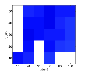
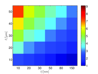
So far we have learned that in Regime III at field strengths $h_{\text{ext}}^{*}\sim d^{2/3}\ell^{-4/3}t^{2/3}$ there is a bifurcation in direction of the unstable mode $\delta m=(0,\delta A\sin(\pi\frac{x_{2}}{\ell})\sin(2\pi\frac{x_{1}}{w^{*}}),0)$. We claim that the concertina pattern grows out of this unstable mode. If so, the experimentally observed period $w^{*}_{\text{exp}}$ should be close to the period $w^{*}$ of the unstable mode. Defining and determining $w^{*}_{\text{exp}}$ is delicate: As $h_{\text{ext}}$ increases (after the critical field $h_{\text{ext}}^{*}$ is passed), there is a continuous transition from the magnetization ripple, see Subsection V, to the concertina pattern, which is far from exactly periodic, and which coarsens subsequently, see Section III. As $w^{*}_{\text{exp}}$ we take the average period as soon as the concertina pattern is discernible to the eye. Figure 11 shows the result of this comparison for a broad range of sample dimensions $\ell$ and $t$ and (therefore) a fairly broad range of periods $w^{*}$: The ratio of the smallest width $\ell$ compared to the largest is $5$, the ration of the smallest thickness $t$ compared to the largest is $15$. The smallest period $w^{*}$ is expected for a thick film of small width, the largest period for a thin film of large width, differing by a factor close to six (neglecting the prediction for the broken or defect samples). The ratio $\frac{w^{*}_{\text{exp}}}{w^{*}}$ of the experimental period with respect to the prediction ranges around two. We basically see this as a confirmation of our hypothesis, namely that the concertina grows out of the oscillatory buckling. Notice that the deviation has a clear trend: $w_{\text{exp}}^{*}$ is larger than $w^{*}$. We give an explanation for this systematic deviation in Section III.

Figure 11: The theoretical period of the unstable mode is in good correspondence to the measurements: The upper image shows the ratio of the experimentally observed period and the period of the unstable mode. The white patches correspond to broken or defect-ridden samples. The lower displays the ratio of the period $w^{*}$ and the smallest period, i.e., $w^{*}(\ell=50\upmu\text{m},t=150\text{nm})$, at all. Both images share the same color map.

I.8 A reduced energy functional

In the forthcoming section we start with the investigation of the type of the bifurcation. For the moment we continue to neglect anisotropy, although it may affect the type of bifurcation as we shall discuss in Section VI. In order to understand the type of bifurcation we now first pass to a reduced model adapted to our Regime III: The form of the unstable mode suggests that the out-of-plane component and the dependence on the thickness variable are negligible, i.e., we assume  $m_{3}\equiv 0$ and $m=m(x_{1},x_{2})$ respectively. Since the unstable mode varies faster in $x_{1}$-direction than in $x_{2}$-direction, we neglect $|\partial_{2}m|^{2}$ with respect to $|\partial_{1}m|^{2}$ in the exchange energy density. Since the oscillation in the sign of the charge density is on smaller length scales in $x_{1}$-direction than in $x_{2}$-direction, we neglect $h_{2}^{2}$ with respect to $h_{1}^{2}+h_{3}^{2}$ in the stray-field energy density, where $H_{\text{stray}}=(h_{1},h_{2},h_{3})$. Finally, since we are interested in small deviations from $m^{*}=(1,0,0)$, we expand $m_{1}=\sqrt{1-m_{2}^{2}}\approx 1-\frac{m_{2}^{2}}{2}$, so that we may neglect $|\nabla m_{1}|^{2}$ with respect to $|\nabla m_{2}|^{2}$ in the exchange energy density. We also use this approximation in the charge density and in the Zeeman energy. Hence (up to an additive constant) we are left with the reduced energy functional

$$E(m_{2})\approx d^{2}t\int_{\Omega^{\prime}}(\partial_{1}m_{2})^{2}\operatorname{d}\!x_{1}\operatorname{d}\!x_{2}\\ +\int_{\text{all space}}(h_{1}^{2}+h_{3}^{2})\;\operatorname{d}\!x_{1}\operatorname{d}\!x_{2}\operatorname{d}\!x_{3}-h_{\text{ext}}\;t\int_{\Omega^{\prime}}m_{2}^{2}\;\operatorname{d}\!x_{1}\operatorname{d}\!x_{2},$$ (7)

where the stray field $H_{\text{stray}}=(h_{1},0,h_{3})$ is determined via

$$\partial_{3}h_{1}-\partial_{1}h_{3}=0,$$

$$\int_{\text{all space}}(h_{1}\partial_{1}\zeta+h_{3}\partial_{3} \zeta)\operatorname{d}\!x_{1}\operatorname{d}\!x_{2}\operatorname{d}\!x_{3}$$

$$\quad=t\int_{\Omega^{\prime}}(-\tfrac{m_{2}^{2}}{2} \partial_{1}\zeta+m_{2}\partial_{2}\zeta)\operatorname{d}\!x_{1}\operatorname{d}\!x_{2}\text{ for all }\zeta,$$ (8)

which is a consequence of the alternative formulation (5). Here, $\Omega^{\prime}$ denotes the in-plane cross section of our sample $\Omega=\Omega^{\prime}\times(0,t)$.

We note that the stray-field energy is only finite if $m_{2}$ vanishes at the lateral long edges, i.e., $m_{2}(x_{1},x_{2})=0$ for $x_{2}=0,\ell$ (as is true for the unstable mode). Notice that (8) can be written as

$$\partial_{1}h_{1}+\partial_{3}h_{3}=0\quad\mbox{for}\;x_{3}\not=0,$$

$$[h_{3}]\;=\;t(-\partial_{1}\tfrac{m_{2}^{2}}{2}+\partial_{2}m_{2})\quad\mbox{for}\;x_{3}=0,$$

where $[h_{3}]$ denotes the jump $h_{3}$ experiences across $x_{3}=0$. This formulation shows that $x_{2}$ is just a parameter in the equations for the stray field, which behaves like a two-dimensional stray field (in the $x_{1}x_{3}$-plane) generated by the “line charge” $t(-\partial_{1}\frac{m_{2}^{2}}{2}+\partial_{2}m_{2})$.

We note that the only non-quadratic term in the energy comes from the non-linear charge distribution $t(-\partial_{1}\frac{m_{2}^{2}}{2}+\partial_{2}m_{2})$. This allows us to derive the scaling of the amplitude of the magnetization: It should be such that both terms in the charge distribution balance. Since in view of the unstable mode the typical $x_{1}$-scale of the variations of $m_{2}$ is given by $w^{*}\sim d^{2/3}\ell^{2/3}t^{-1/3}$, whereas the typical $x_{2}$-scale of variations of $m_{2}$ is given by the sample width $\ell$, the contributions $\partial_{1}\frac{m_{2}^{2}}{2}$ and $\partial_{2}m_{2}$ balance provided the amplitude of $m_{2}$ scales as $d^{2/3}\ell^{-1/3}t^{-1/3}$. This suggests the following non-dimensionalization of length, and reduced units for the stray field and the magnetization:

$$\begin{split}x_{1}=d^{2/3}\ell^{2/3}{t}^{-1/3}\hat{x}_{1},\;x_{2}&=\ell\hat{x}_{2},\;x_{3}=d^{2/3}\ell^{2/3}{t}^{-1/3}\hat{x}_{3},\\ h_{1}=d^{2/3}\ell^{-4/3}t^{2/3}\hat{h}_{1},&\quad h_{3}=d^{2/3}\ell^{-4/3}t^{2/3}\hat{h}_{3},\quad\\ m_{2}=d^{2/3}&\ell^{-1/3}t^{-1/3}\hat{m}_{2}.\end{split}$$ (9)

After the reduction leading to (7), only the stray-field depends on the $x_{3}$-component for which the relevant length scale is of course the wavelength of the oscillation, cf. Section I.6, III and Figure 9 – the relevant length scale in case of the magnetization leading to the reduction (7) is of course the film thickness $t$. If we also rescale the external field – in the same way as the stray field – and the energy itself according to

$$h_{\text{ext}} =d^{2/3}\ell^{-4/3}t^{2/3}\hat{h}_{\text{ext}},$$ (10)

$$E =d^{8/3}\ell^{-1/3}t^{2/3}\hat{E},$$ (11)

we obtain the reduced rescaled energy functional

$$\hat{E}(\hat{m}_{2})=\int_{\hat{\Omega}^{\prime}}(\hat{\partial}_{1}\hat{m}_{2})^{2}\operatorname{d}\!\hat{x}_{1}\operatorname{d}\!\hat{x}_{2}\\ +\int_{\text{all space}}(\hat{h}_{1}^{2}+\hat{h}_{3}^{2})\operatorname{d}\!\hat{x}_{1}\operatorname{d}\!\hat{x}_{2}\operatorname{d}\!\hat{x}_{3}-\hat{h}_{\text{ext}}\int_{\hat{\Omega}^{\prime}}\hat{m}_{2}^{2}\operatorname{d}\!\hat{x}_{1}\operatorname{d}\!\hat{x}_{2},$$ (12)

where the reduced rescaled stray field is determined by

$$\hat{\partial}_{1}\hat{h}_{1}+\hat{\partial}_{3}\hat{h}_{3}=0\quad\mbox{for}\;\hat{x}_{3}\not=0,$$

$$[\hat{h}_{3}]\;=\;(-\hat{\partial}_{1}\tfrac{\hat{m}_{2}^{2}}{2}+\hat{\partial}_{2}\hat{m}_{2})\quad\mbox{for}\;\hat{x}_{3}=0,$$

The reduced rescaled formulation shows that the reduced energy functional contains just one non-dimensional parameter, namely the reduced external field $\hat{h}_{\text{ext}}$ – instead of four parameters (exchange length, sample dimensions and $h_{\text{ext}}$) for the full model. Moreover, the vector field $m=(m_{1},m_{2},m_{3})$, function of three variables $(x_{1},x_{2},x_{3})$, has been replaced by the scalar function $\hat{m}_{2}$, function of two variables $(\hat{x}_{1},\hat{x}_{2})$. Finally, the computation of the stray field is a two-dimensional computation (in $(\hat{x}_{1},\hat{x}_{3})$ only with $\hat{x}_{2}$ as a parameter) instead of a three-dimensional one. All this simplifies both the theoretical treatment and the numerical simulation. For clarity, we will mostly discuss our results in the rescaled variables (12) – and only occasionally return to the original variables, mostly for comparison with the experiment and when we take into account anisotropy.

In Theorem 3 in [6, p.233], we rigorously show that the reduced energy functional is the scaling limit of the renormalized full micromagnetic energy in Regime III.

I.9 Bifurcation

We now return to the issue of the type of bifurcation on the level of the reduced model. Let us note that the Hessian of the reduced model in $\hat{m}_{2}\equiv 0$ can be explicitly diagonalized and the first unstable mode is given by $\hat{m}_{2}^{*}=\sin(\pi\hat{x}_{2})\sin(2\pi\tfrac{x_{1}}{\hat{w}^{*}})$, where $\hat{w}^{*}=(32\pi)^{1/3}$ in agreement with (6). The reduced critical field is given by

$$\hat{h}_{\text{ext}}^{*}=3\left(\tfrac{\pi}{2}\right)^{4/3}.$$ (13)

In order to determine the type of bifurcation, we have to investigate the energy functional $\hat{E}$ close to the one-dimensional subspace $\{A\hat{m}_{2}^{*}\}$ generated by the unstable mode $\hat{m}_{2}^{*}$. Because of the invariance of both the energy $\hat{E}$ and the unstable mode $\hat{m}_{2}^{*}$ under the transformation ($\hat{m}_{2}\leadsto-\hat{m}_{2}$ and $\hat{x}_{2}\leadsto 1-\hat{x}_{2}$), all odd terms in the amplitude $A$ in the expansion of $\hat{E}(A\hat{m}_{2}^{*})$ vanish. In particular the cubic term vanishes so that the bifurcation is degenerate.

This degeneracy of the bifurcation means that at the critical field strength $\hat{h}_{\text{ext}}^{*}$, the first non-vanishing term in the expansion of $\hat{E}(A\hat{m}_{2}^{*})$ with respect to $A$ is at least quartic. Hence it is not sufficient to consider $\hat{E}$ just along the linear space $\{A\hat{m}_{2}^{*}\}$ but it has to be analyzed along a curve $\{A\hat{m}_{2}^{*}+A^{2}\hat{m}_{2}^{**}\}$ in configuration space. Indeed, the curvature direction $\hat{m}_{2}^{**}$ affects the quartic term in the expansion and has to be determined such that $\hat{E}$ is minimal. This minimization problem of the coefficient of the quartic term is quadratic in $\hat{m}_{2}^{**}$ and thus can be solved explicitly. We obtain

$$\hat{m}_{2}^{**}=-\tfrac{1}{10}(\tfrac{2}{\pi})^{1/3}\sin(2\pi{x_{2}})\sin(4\pi\tfrac{x_{1}}{\hat{w}^{*}}),$$

which leads to a negative coefficient of the quartic term in the expansion of $\hat{E}$, namely

$$\hat{E}(A\hat{m}_{2}^{*}+A^{2}\hat{m}_{2}^{**})\approx(\hat{h}_{\text{ext}}-\hat{h}_{\text{ext}}^{*})\left(\tfrac{\pi}{2}\right)^{1/3}A^{2}-\tfrac{\pi}{640}A^{4}.$$ (14)

The negative quartic coefficient implies that the bifurcation is subcritical or of first order. Subcriticality entails that close to $\hat{m}_{2}\equiv 0$, there are only unstable stationary points for $\hat{h}_{\text{ext}}$ slightly below $\hat{h}_{\text{ext}}^{*}$, and no stationary points close to $\hat{m}_{2}\equiv 0$ for $\hat{h}_{\text{ext}}$ slightly above $\hat{h}_{\text{ext}}^{*}$, cf. Figure 12.

Figure 12: Energy landscape close to the bifurcation. The loss of stability at the critical field leads to a first-order phase transition – on a large scale however the energy is coercive.

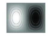
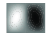
At first sight it is surprising that the stray-field energy contribution to $\hat{E}$, which gives rise to the only quartic term in $\hat{m}_{2}$, and clearly is non-negative, may nevertheless allow for a negative coefficient in front of the quartic term in the expansion (14). This comes from the fact that the two terms in the charge density $-\hat{\partial}_{1}\frac{\hat{m}_{2}^{2}}{2}+\hat{\partial}_{2}\hat{m}_{2}$ interact, giving rise to a cubic term in $\hat{m}_{2}$ (quartic in $A$), which indeed allows for cancellations. The way how this operates is better understood in physical space: The term $\hat{m}_{2}^{**}$ in $A\hat{m}_{2}^{*}+A^{2}\hat{m}_{2}^{**}$ (the curvature direction in configuration space) induces a tilt of the symmetric charge distribution of $A\hat{m}_{2}^{*}$, see Figure 13. This tilt brings opposite charges closer together, thereby reducing the stray field energy – while increasing the exchange energy to a lesser amount.

Figure 13: Unstable mode $\{A\hat{m}_{2}^{*}\}$ and additional curvature correction $\{A\hat{m}_{2}^{*}+A^{2}\hat{m}_{2}^{**}\}$ with generated charges.

Since the bifurcation is first order, it is not obvious whether minimizers of the reduced energy functional can be related to the unstable mode. In particular, this finding sheds doubt on our hypothesis that the concertina pattern inherits the period of the unstable mode. It is even not obvious whether minimizers of the reduced energy functional exist at all. However, one can show that the reduced energy is coercive for all values of the external field $\hat{h}_{\text{ext}}$, see Theorem 4 in [6, p.236]. This in particular implies that there always exists a global minimizer of the reduced energy – which corresponds to a local minimizer of the original energy (1), see Theorem 5 in [6, p.237] – in particular for fields larger than the critical field. But it is not immediately clear how these minimizers relate to the unstable mode.

It is natural to resort to numerical simulations; details on the discretization and the algorithms are provided in Section IV. To confirm the conjecture that the unstable mode in Regime III is indeed related to the concertina pattern, we use a numerical path-following algorithm in order to compute the bifurcation branch. Figure 14 shows the outcome of the numerical simulations. As expected due to the coercivity of the energy functional, we find a turning point as we follow the bifurcation branch. The turning point is located at a field which is just slightly – about one percent – smaller than the critical field. After the turning point the configurations become stable, at least under perturbations of the same period.

Figure 14: Numerical simulations: The $\hat{w}^{*}$-periodic branch close to the bifurcation and the pattern at the indicated fields. The gray scales encode the $m_{2}$ component but are not comparable. The whole spectrum is exhausted so that the structure of the pattern can best be resolved. By $\langle\hat{m}_{2}^{2}\rangle^{1/2}$ we denote the spatial root mean square of $\hat{m}_{2}$, i.e., the amplitude of the average magnetization.

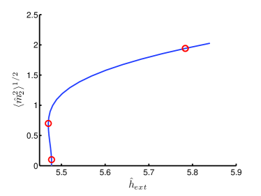
As the field increases beyond the turning point, the unstable mode develops into a domain pattern of concertina type with its typical scale separation between the wall width and the domain size, cf. Figure 15. We thus find a continuous transition from the unstable mode to the concertina pattern – confirming our hypothesis.

Figure 15: Numerical simulations: The $\hat{w}^{*}$-periodic concertina pattern exhibits a clear scale separation as $\hat{h}_{\text{ext}}$ increases; $\hat{h}_{\text{ext}}=6.84,\,23.2,\,40.1,\,57.3$ from left to right. The gray scales linearly encode the $\hat{m}_{2}$-component and are comparable.

The numerical simulations lead to the conjecture that the magnetization in a perfectly homogeneous, isotropic sample exhibits a first-order phase transition from the uniformly magnetized state to the concertina state of period $w^{*}$ at the critical field. Clearly this does not explain the deviation of the average wavelength in the experimental measurements from the theoretical prediction. Before we address this deviation we now introduce a sharp-interface model, so-called domain theory, that is used to investigate the further transformation of the concertina for large external fields $\hat{h}_{\text{ext}}\gg 1$, in particular the coarsening, see Subsections III.1, III.2, and III.3. Our explanation of the coarsening will also provide an understanding of the initial deviation of the period, cf. Subsection III.4.

II Domain theory

In the numerical simulations, we observe for large external fields a clear scale separation between domains, where the magnetization is almost constant, and walls, in which the magnetization quickly turns, cf. Figure 15. This suggests the application of a sharp-interface model, namely domain theory. In the following we first discuss admissible Ansatz functions and then derive their energy within domain theory. This leads to a model which only depends on a small number of parameters in configuration space that is used in Section III and VI in order to get a better understanding of the coarsening of the concertina.

Figure 16: Domain theory: The mesoscopic charge-free Ansatz function.

On a mesoscopic scale, the computed magnetization is close to a piecewise constant magnetization of amplitude $\hat{m}_{2}^{0}$, i.e., $\hat{m}_{2}=\pm\hat{m}_{2}^{0}$ in the quadrangular domains and $\hat{m}_{2}=0$ in the triangular domains as indicated in Figure 16. We observe that the angles in the pattern are related to the amplitude of the magnetization $\hat{m}_{2}^{0}$, cf. Figure 15; approximately we have that $\sin\alpha=2\hat{m}_{2}^{0}$. This is related to the fact that the (reduced) stray-field energy is strongly penalized for large fields, as we shall explain now. In fact, the piecewise constant magnetization is a distributional solution of

$$-\hat{\partial}_{1}(\tfrac{\hat{m}_{2}^{2}}{2})+\hat{\partial}_{2}\hat{m}_{2}=0,$$ (15)

which means that the normal component of the vector field $(-\tfrac{\hat{m}_{2}^{2}}{2},\hat{m}_{2})$ is continuous across the interfaces – this is a version of the Rankine-Hugoniot condition in the theory of conservation laws. This condition obviously holds in case of the vertical walls. In case of the diagonal walls the condition

$$0=[\hat{\nu}\cdot(-\tfrac{\hat{m}_{2}^{2}}{2},\hat{m}_{2})]=\hat{\nu}\cdot(-\tfrac{1}{2}(\hat{m}_{2}^{0})^{2},\hat{m}_{2}^{0}),$$ (16)

where $\hat{\nu}$ denotes the normal of the diagonal wall as depicted in Figure 16, is equivalent to $\sin\alpha=2\hat{m}_{2}^{0}$. Therefore the piecewise constant magnetization satisfying (16) mesoscopically carries no stray-field energy. Of course, on a microscopic scale equation (15) does not hold: The continuous transition in the wall generates a right hand side, i.e., dipolar charges. Note that walls have to form since (15) does not allow for non-trivial smooth solutions with boundary data $\hat{m}_{2}=0$.

Within domain theory we therefore consider piecewise constant magnetizations of concertina type of period $\hat{w}$ and of amplitude $\hat{m}_{2}=\pm\hat{m}_{2}^{0}$ in the quadrangular and $\hat{m}_{2}=0$ in the triangular domains, s.t. (16) holds. Since the angles are fixed by (16), admissible configurations are characterized by two parameters, namely the amplitude of the magnetization $\hat{m}_{2}^{0}$ and the width of the folds $\hat{w}$.

Figure 17: Domain theory and numerical simulations: The domain theoretic prediction for the optimal amplitude (red) and the computed amplitude based on the reduced model (blue). For the reduced model we display the amplitude, i.e., the maximal value which is attained in the quadrangular domain.

The energy which discriminates between these solutions is given by the total wall energy, which is an appropriate line-energy density integrated over the interfaces, augmented by Zeeman energy. The specific line energy is a function of the jump $[\hat{m}_{2}]=2\hat{m}_{2}^{0}$ of the magnetization across the wall – an infinitesimal version of the wall angle. Due to the shear invariance of the reduced energy, namely

$$\hat{x}_{1}\,=\,s\,\hat{x}_{2}+\tilde{x}_{1},\quad\hat{x}_{2}\,=\,\tilde{x}_{2},\quad\hat{m}_{2}\,=\,\tilde{m}_{2}-s,$$ (17)

by which a diagonal wall can be transformed into a vertical wall – for the choice of $s=\pm\frac{\hat{m}_{2}^{0}}{2}$ – the specific line energy can be obtained by restricting the reduced energy functional to one-dimensional transitions with boundary data $\pm\hat{m}_{2}^{0}$ in case of the vertical walls and $\pm\frac{\hat{m}_{2}^{0}}{2}$ in case of the diagonal walls. The optimal transition layers are low-angle Néel walls whose line-energy density scales as

$$\hat{e}_{\text{wall}}\big{(}\tfrac{[\hat{m}_{2}]}{2}\big{)}\,=\,\hat{e}_{\text{wall}}(\hat{m}_{2}^{0})\,\approx\,\tfrac{\pi}{8}(\hat{m}_{2}^{0})^{4}\ln^{-1}\frac{\hat{w}_{\text{tail}}}{\hat{w}_{\text{core}}},$$

where $\hat{w}_{\text{tail}}$ and $\hat{w}_{\text{core}}$ are the two characteristic length scales of the Néel wall, [8, Section 6]. The tails of the Néel wall decay only logarithmicly and spread as much as possible. In case of the concertina pattern, they are only limited by the neighboring walls – thus $\hat{w}_{\text{tail}}\approx\frac{\hat{w}}{4}$. A more careful inspection shows that the core width decreases with increasing jump size, more precisely $\hat{w}_{\text{core}}\sim(\hat{m}_{2}^{0})^{-2}$, see [18, Subsection 3.5.5]. Hence we obtain

$$\hat{e}_{\text{wall}}(\hat{m}_{2}^{0})\,\approx\,\tfrac{\pi}{8}(\hat{m}_{2}^{0})^{4}\ln^{-1}(\hat{w}(\hat{m}_{2}^{0})^{2}).$$ (18)

With the rescaling (9) and (10) this turns into

$$e_{\text{wall}}(m_{2}^{0})\,\approx\,\tfrac{\pi}{8}t^{2}(m_{2}^{0})^{4}\ln^{-1}(d^{-2}tw(m_{2}^{0})^{2}).$$ (19)

Within the class of admissible magnetizations, the domain theoretic energy becomes a function of only three parameters, namely $\hat{m}_{2}^{0}$, $\hat{w}$ and $\hat{h}_{\text{ext}}$. To see this, notice that one period of the pattern in Figure 16 contains

• two vertical walls of height $1-\frac{\hat{w}}{\hat{m}_{2}^{0}}$ and of jump size $2\,\hat{m}_{2}^{0}$, leading to an energy contribution of $2\,(1-\frac{\hat{w}}{\hat{m}_{2}^{0}})\,\hat{e}_{\text{wall}}(\hat{m}_{2}^{0})$,

• four diagonal walls of projected height $\frac{\hat{w}}{\hat{m}_{2}^{0}}$ and of jump size $\hat{m}_{2}^{0}$, leading to an energy contribution of $4\,\frac{\hat{w}}{\hat{m}_{2}^{0}}\,\hat{e}_{\text{wall}}(\frac{\hat{m}_{2}^{0}}{2})$,

• two quadrangular domains of total area $\hat{w}-\tfrac{\hat{w}^{2}}{\hat{m}_{2}^{0}}$, leading to a Zeeman energy of $-\hat{h}_{\text{ext}}(\hat{m}_{2}^{0})^{2}\,(\hat{w}-\tfrac{\hat{w}^{2}}{\hat{m}_{2}^{0}})$.

Hence, the total domain energy per period in rescaled variables is given by

$$\hat{E}_{\text{domain}}(\hat{m}_{2}^{0}, \hat{h}_{\text{ext}},\hat{w})\,$$

$$= \;2\,(1-\tfrac{\hat{w}}{\hat{m}_{2}^{0}})\,\hat{e}_{\text{wall}}(\hat{m}_{2}^{0})+4\,\tfrac{\hat{w}}{\hat{m}_{2}^{0}}\,\hat{e}_{\text{wall}}\big{(}\tfrac{\hat{m}_{2}^{0}}{2}\big{)}$$

$$-\hat{h}_{\text{ext}}(\hat{m}_{2}^{0})^{2}(\hat{w}-\tfrac{\hat{w}^{2}}{\hat{m}_{2}^{0}}).$$ (20)

Within the original scaling the domain theoretic energy takes the form of

$$E_{\text{domain}}(m_{2}^{0}, h_{\text{ext}},w)$$

$$= \;2\big{(}\ell-\tfrac{w}{m_{2}^{0}}\big{)}\,e_{\text{wall}}(m_{2}^{0})+4\,\tfrac{w}{m_{2}^{0}}\,e_{\text{wall}}\big{(}\tfrac{m_{2}^{0}}{2}\big{)}$$

$$-h_{\text{ext}}(m_{2}^{0})^{2}\,t\left(w\ell-\tfrac{w^{2}}{m_{2}^{0}}\right).$$ (21)

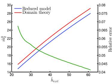
First of all we apply (20) to derive the optimal amplitude of the $\hat{w}^{*}$-periodic concertina pattern as a function of the external field $\hat{h}_{\text{ext}}$ by optimizing the energy in $\hat{m}_{2}^{0}$. Of course, domain theory is only applicable and thus a good approximation for the reduced model for $\hat{h}_{\text{ext}}\gg 1$ in which case there is a clear scale separation between walls and domains. Figure 17 shows that in this case domain theory is in good agreement with our numerical simulations.

Before we go on with the analysis of domain theory let us emphasize that the experimentally observed concertina is of course not of uniform period and equal amplitude as our domain theoretic Ansatz above. As shown in Figure 18, there are also oblique piecewise constant weak solutions of (15). Nevertheless this class of Ansatz functions is very rigid: An elementary calculation shows that the location of the interior triplet $A_{0}$ is uniquely determined by the jump condition (16), if the distance between the boundary triplet $A_{2}$ and $A_{1}$, and $\hat{m}_{2}^{1}$ and $\hat{m}_{2}^{2}$ on both sides are given. Hence the continuation of the pattern is uniquely determined if either the amplitude in the next quadrangular domain or the location of the next triplet, i.e., the width of the next quadrangular domain, is prescribed.

Figure 18: Domain theory: Generalized tilted Ansatz function.

III Coarsening of the concertina pattern

III.1 Domain theory: The optimal period of the concertina pattern for large external fields

Experiments show an increase in the average concertina period $w$ as the external field $h_{\text{ext}}$ is increased after the pattern has formed, see Figure 2. The general tendency that the optimal period $w$ is an increasing function of $h_{\text{ext}}$ can be understood on the basis of domain theory in the reduced variables $\hat{m}_{2}^{0}$, $\hat{h}_{\text{ext}}$ and $\hat{w}$. By optimizing the energy per unit length with respect to the period $\hat{w}$ and the amplitude $\hat{m}_{2}^{0}$ of the transversal component, we obtain the following scaling of the optimal period of the pattern as a function of the external field

$$\hat{w}_{a}(\hat{h}_{\text{ext}})\sim\hat{h}_{\text{ext}}\ln\hat{h}_{\text{ext}}\quad\hat{h}_{\text{ext}}\gg 1.$$ (22)

In particular we find that the optimal period increases with increasing field $\hat{h}_{\text{ext}}$ – the $a$ in $w_{a}$ stands for absolute minimizer. Domain theory also yields the (same) scaling behavior for the optimal transversal component of the magnetization

$$\hat{m_{2}}_{a}(\hat{h}_{\text{ext}})\sim\hat{h}_{\text{ext}}\ln\hat{h}_{\text{ext}}\quad\hat{h}_{\text{ext}}\gg 1.$$ (23)

We note that both scalings have also been confirmed by a rigorous asymptotic analysis of the reduced energy functional (12) which does not rely on a simple concertina Ansatz, cf. Theorem 1 in [17, p.147]. Moreover, numerical simulations of the reduced energy show that the optimal period increases with $\hat{h}_{\text{ext}}$ also for external fields close to the critical field, see Figure 19. The optimal period shown in this diagram was computed by minimizing the energy per unit length both with respect to the magnetization and the period, for varying external field.

Figure 19: Numerical simulations: The optimal period of the concertina pattern as a function of the external field computed on the basis of the reduced model.

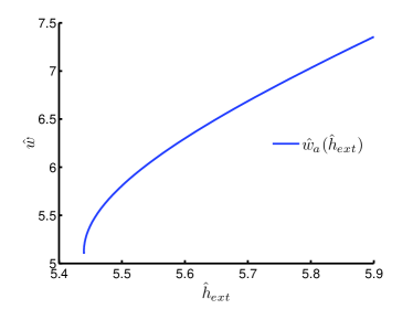
III.2 Coarsening: A modulation instability

Although the above analysis predicts that the optimal period $\hat{w}_{a}$ increases as the field $\hat{h}_{\text{ext}}$ increases, it does not explain why and in which way a concertina pattern of period $\hat{w}$ becomes unstable as $\hat{h}_{\text{ext}}$ increases. We will see that both the increasing period for large fields and the deviation of the initial period close to critical field from the one of the unstable mode are due to an instability under long wavelength modulations of the pattern. The mechanism behind the instability is the following: Given $\hat{h}_{\text{ext}}$ and a period $\hat{w}$, an optimization in the transversal component $\hat{m}_{2}$ yields that the optimal energy per period $\hat{E}_{\text{opt}}(\hat{h}_{\text{ext}},\hat{w})$ is a concave function in $\hat{w}$ if $\hat{h}_{\text{ext}}$ is sufficiently large. The concavity suggests – as depicted in Figure 20 – that the concertina pattern of a uniform period $\hat{w}$ becomes unstable towards perturbations which increase the period to $\hat{w}+\epsilon$ and the corresponding amplitude of the transversal component to $\hat{m}_{2}^{0}(\hat{w}+\epsilon)$ in some folds, and decrease the period to $\hat{w}-\epsilon$ and the amplitude to $\hat{m}_{2}^{0}(\hat{w}-\epsilon)$ it in other folds. This modulation eventually leads to the collapse of the smaller folds, i.e., the coarsening. However, in view of the non-local character of the stray-field energy, it is not clear whether this simplified picture, i.e., that the energy of the modulation amounts to the modulation of the energy, applies. As we shall see in Subsection III.3, a modulation of the period on a very long length scale overcomes this objection. Thus the concavity of the minimal energy implies an instability under long wavelength modulations of the pattern.

Figure 20: Concavity of the minimal energy per period implies an instability under modulation of the wavelength.

In order to derive the concavity of the minimal energy we apply domain theory for large external fields in Subsection III.3 and an extended bifurcation analysis close to the critical field in Subsection III.4. We will see that both asymptotics match the results of the numerical simulation of our reduced model.

Let us mention that the modulation instability of the concertina pattern is closely related to the so-called Eckhaus instability which was discovered in the context of non-linear instabilities in convective systems leading to a change in wavelength of the observed periodic pattern, cf. [9].

III.3 Bloch-wave theory: Instability with increasing field

As indicated above, not only the optimal period but also the coarsening can be explained on the basis of domain theory for large external fields $\hat{h}_{\text{ext}}\gg 1$. This relies on the optimal energy per period $\min_{\hat{m}_{2}}\hat{E}_{\text{domain}}(\hat{m}_{2},\hat{h}_{\text{ext}},\hat{w})$. For periods $\hat{w}$ much smaller than the optimal period at some value of the external field $\hat{h}_{\text{ext}}$, i.e., $\hat{w}\ll\hat{h}_{\text{ext}}\ln\hat{h}_{\text{ext}}$, we find that

$$\min_{\hat{m}_{2}}\hat{E}_{\text{domain}}(\hat{m}_{2},\hat{h}_{\text{ext}},\hat{w})\sim-\hat{h}_{\text{ext}}^{2}\hat{w}^{2}\ln(\hat{h}_{\text{ext}}\hat{w}^{2}).$$ (24)

In particular, the optimal energy per period in (24) is concave in the period $\hat{w}$. Although domain theory therefore suggests an instability under wavelength modulation for periods which are much smaller than the optimal period, it is too rigid to allow for such a type of perturbation, even in the class of generalized Ansatz functions, cf. Figure 18.

It is rather on the level of the reduced model that it can be seen that the concavity translates into an instability (despite the potentially long-range interactions via the stray field). Indeed, a so-called Bloch-wave analysis of the reduced model shows that the concavity is in a one-to-one correspondence with an instablitity under long wavelength modulations of the pattern. In the Bloch-wave analysis one considers $N\hat{w}$-periodic eigenfunctions of the Hessian of the form

$$\delta\hat{m}_{2}\;=\;e^{-i\hat{x}_{1}\hat{k}_{1}}\,\delta\hat{m}_{2}^{\hat{k}_{1}}$$

with wavenumber $\hat{k}_{1}=\frac{2\pi}{N\hat{w}}$ and $N$ some large integer and where $\delta\hat{m}_{2}^{\hat{k}_{1}}$ is $\hat{w}$-periodic with respect to $\hat{x}_{1}$, i.e., one condisders sinusiodal modulations of some suitable $\hat{w}$-periodic function. An asymptotic expansion of

$$\operatorname{Hess}\hat{E}(\hat{m}_{2})(e^{-i\hat{x}_{1}{\hat{k}_{1}}}\delta\hat{m}_{2}^{\hat{k}_{1}})=\lambda^{\hat{k}_{1}}e^{-i\hat{x}_{1}{\hat{k}_{1}}}\,\delta\hat{m}_{2}^{\hat{k}_{1}}$$ (25)

for small wavenumbers $\hat{k}_{1}\ll 1$, i.e., $N\gg 1$, shows that the first eigenvalue can be related to the second derivative of the optimal energy per period $\hat{E}_{\text{opt}}=\min_{\hat{m}_{2}}\hat{E}$. More precisely, one can show that the eigenvalue possesses the expansion

$$\lambda^{\hat{k}_{1}}\approx c_{0}\;{\hat{k}_{1}}^{2}\frac{\operatorname{d}\!^{2}}{\operatorname{d}\!\hat{w}^{2}}\hat{E}_{\text{opt}}(\hat{h}_{\text{ext}},\hat{w})\quad\text{for}\quad{\hat{k}_{1}}\ll 1,$$

where $c_{0}$ denotes a constant that depends on $\hat{m}_{2}$, see [19, Theorem 5.1]. This shows that the concavity of $\hat{E}_{\text{opt}}(\hat{h}_{\text{ext}},\hat{w})$ with respect to the period $\hat{w}$ implies that the concertina pattern of a given period $\hat{w}$ is unstable. Domain theory predicts that the marginally stable period $\hat{w}_{s}$, i.e., $\hat{w}_{s}$ such that  $\frac{\operatorname{d}\!^{2}}{\operatorname{d}\!\hat{w}^{2}}\hat{E}_{\text{opt}}(\hat{h}_{\text{ext}},\hat{w}_{s})=0$, scales as $\hat{w}_{s}\sim\hat{h}_{\text{ext}}\ln\hat{h}_{\text{ext}}$, cf. (24) – we note that the $s$ in $w_{s}$ stands for marginally stable. Figure 21 displays the optimal and the marginally stable period computed on the basis of the reduced energy functional.

Figure 21: Numerical simulations: Comparison of the optimal and marginally stable period of the concertina pattern as a function of the external field – both computed on the basis of the reduced model. In the region below the red curve the minimal energy per period is concave and thus a concertina of that period is unstable and coarsens.

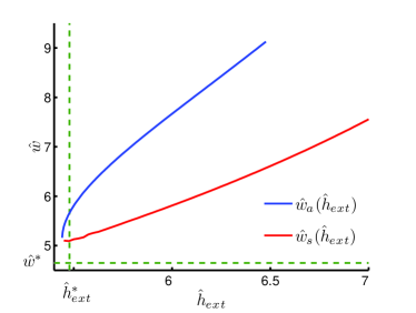
Figure 22 shows that the computation of the optimal and the marginally stable period on the basis of domain theory matches the numerical simulations on the basis of the reduced model.

Figure 22: Numerical simulations and domain theory: The optimal and marginally stable period computed on the basis of the reduced model (dashed) match the predictions on the basis of domain theory in the regime $\hat{h}_{\text{ext}}\gg 1$.

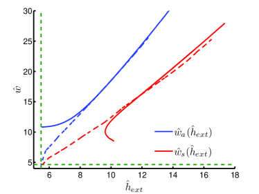
III.4 Bifurcation analysis: Instability for small fields

The numerical computations, cf.  Figure 21, show that the optimal energy per period is concave not only for large external fields as predicted by domain theory. In fact, we extract from our numerical data that $\frac{\operatorname{d}\!^{2}}{\operatorname{d}\!\hat{w}^{2}}\hat{E}_{\text{opt}}(\hat{h}_{\text{ext}},\hat{w}^{*})$ is negative also for small external fields up to the turning point. This is consistent with the numerical computation of the eigenvalue $\lambda^{N}$ based on the asymptotic expansion of equation (25). Hence, the Bloch-wave analysis implies that the $\hat{w}^{*}$-periodic concertina pattern is unstable under long wavelength modulations close to the critical field.

This qualitatively explains the trend in the deviation of the initial concertina period $w^{*}_{\text{exp}}$ from the period of the unstable mode, see Subsection I.7. Close to the critical field, the concavity can be confirmed with the help of an asymptotic bifurcation analysis. To see this, we extend our Ansatz from Section I.9 and take into account small deviations of the wavenumber $\hat{k}=\hat{k}^{*}+\hat{\delta k}$. As we have seen in (14) in Section I.9, the quartic coefficient in the energy expansion, namely $\frac{\pi}{640}$, is small compared to the second order coefficient and the scale of the reduced external field. Due to that degeneracy it is necessary to additionally take into account a contribution of cubic order in the perturbation of $\hat{m}_{2}=0$, i.e., we use the extended Ansatz

$$\hat{m}_{2}\approx A\hat{m}_{2}^{*}+A^{2}\hat{m}_{2}^{**}+A^{3}\hat{m}_{2}^{***}.$$

Optimizing the coefficients in the expansion of the energy with respect to $A$ subsequently in $\hat{m}_{2}^{**}$ and $\hat{m}_{2}^{***}$ leads to an expansion of the energy density of the form

$$\tfrac{\hat{k}}{2\pi}\hat{E}(A \hat{m}_{2}^{*}+A^{2}\hat{m}_{2}^{**}+A^{3}\hat{m}_{2}^{***})$$

$$\approx \tfrac{1}{4}(\hat{h}_{\text{ext}}^{*}(\hat{k})-\hat{h}_{\text{ext}})A^{2}-c_{4}(\hat{k})A^{4}+c_{6}(\hat{k})A^{6},$$

where $c_{4}(\hat{k}^{*})=\frac{\pi}{640}\frac{\hat{k}^{*}}{2\pi}$ in accordance with (14). Hence under the assumption that $c_{4}(\hat{k}^{*})\approx 0.00105$ is small, the energy density to leading order can be approximated by

$$\tfrac{\hat{k}}{2\pi}\hat{E} (A\hat{m}_{2}^{*}+A^{2}\hat{m}_{2}^{**}+A^{3}\hat{m}_{2}^{***})$$

$$\approx \tfrac{1}{4}\big{(}\tfrac{\operatorname{d}\!^{2}}{\operatorname{d}\!\hat{k}^{2}}\hat{h}_{\text{ext}}^{*}(\hat{k})_{|\hat{k}=\hat{k}^{*}}\tfrac{\hat{\delta k}^{2}}{2}+\delta\hat{h}_{\text{ext}}\big{)}A^{2}$$

$$-(c_{4}(\hat{k}^{*})+\tfrac{\operatorname{d}\!}{\operatorname{d}\!\hat{k}}c_{4}(\hat{k})_{|\hat{k}=\hat{k}^{*}}\hat{\delta k})A^{4}+c_{6}(\hat{k}^{*})A^{6}.$$ (26)

The numerical values of the coefficients are given by

$$\tfrac{\operatorname{d}\!^{2}}{\operatorname{d}\!\hat{k}^{2}}\hat{h}_{\text{ext}}^{*}(\hat{k})_{|\hat{k}=\hat{k}^{*}}=3,$$

$$\tfrac{\operatorname{d}\!}{\operatorname{d}\!\hat{k}}c_{4}(\hat{k})_{|\hat{k}=\hat{k}^{*}}\approx-0.0217,$$

$$c_{6}(\hat{k}^{*})\approx 0.000207.$$

Notice that $c_{6}(\hat{k}^{*})$ is positive, confirming the numerically observed turning point of the $\hat{w}^{*}$-periodic branch. Obviously, the asymptotic expansion displays an asymmetric behavior in $\hat{\delta k}$; the energy decreases for $\hat{\delta k}<0$. Based on the expansion (26), one can characterize the optimal wavenumber and the optimal period. We note that the concavity of the minimal energy per period as a function of the period is equivalent to the concavity of the energy density as a function of the wavenumber $\hat{k}$:

$$\tfrac{\operatorname{d}\!^{2}}{\operatorname{d}\!\hat{w}^{2}}\hat{E}(\hat{w})\;=\;\tfrac{\hat{k}^{3}}{(2\pi)^{2}}\tfrac{\operatorname{d}\!^{2}}{\operatorname{d}\!\hat{k}^{2}}\Big{(}\hat{k}\hat{E}\big{(}\tfrac{2\pi}{\hat{k}}\big{)}\Big{)}.$$

Figure 23 shows the optimal period and the marginally stable period calculated on the basis of (26). We read off that the $\hat{w}^{*}$-periodic concertina pattern is indeed unstable at the critical field.

Figure 23: Bifurcation analysis: The optimal and marginally stable period as a function of the external field obtained on the basis on the extended bifurcation analysis.

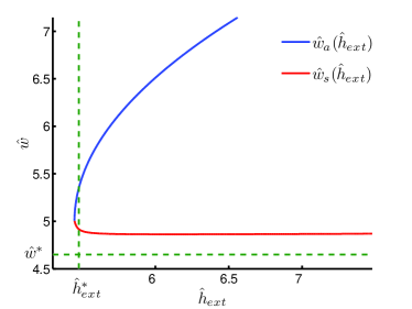
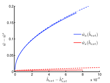
A comparison between Figure 21 and Figure 23 shows that the predictions on the basis of the asymptotic expansion differ from the optimal and the marginally stable period computed on the basis of the reduced model, compare for example the scale of the external field. This deviation is related to our assumption that the quartic coefficient is small so that the energy can be approximated by (26). On the other hand, Figure 24 shows that the asymptotics match the reduced model if we add a quartic contribution $+\frac{\hat{Q}}{4}\int m_{2}^{4}$ to the reduced energy where the value of the parameter $\hat{Q}$ is such that the contribution cancels $c_{4}(\hat{k}^{*})$ in (26) ( which happens $\hat{Q}\approx 0.03$). We will see later that such an additional quartic contribution has a physical meaning if we take into account a uniaxial anisotropy, see Section VI. It turns out that $\hat{Q}$ corresponds to an appropriately rescaled quality factor $Q$.

Figure 24: Numerical simulations and bifurcation analysis: The prediction on the basis of the reduced model (dashed) matches the prediction on the basis of the extended bifurcation analysis for a near-degenerate value of $\hat{Q}=0.0295$ close to $\hat{Q}^{*}\approx 0.03$, cf. Section VI.

III.5 Numerical bifurcation analysis: Type of secondary instability and downhill path in energy landscape

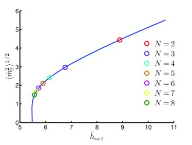
With the help of a bifurcation-detection algorithm we are able to compute at which field the $\hat{w}^{*}$-periodic concertina becomes unstable under $N\hat{w}^{*}$-periodic perturbations while we follow the primary branch. Figure 25 shows the secondary critical fields; as expected (cf. Subsection III.4 and Figure 21) the secondary instability approaches the turning point as the integer $N$ increases. We note that it is reached for finite $N$.

Figure 25: Numerical simulations: The appearance of the secondary instability under $N\hat{w}^{*}$-periodic perturbations as a function of $N$. The critical field for $N=8$ is given by $5.602$.

In the following we want to study in which way the concertina pattern becomes unstable. We first present the outcome of the computation of the secondary bifurcation branches. We point out that due to the symmetries of the pattern, the bifurcations are not simple in the sense that more than one branch bifurcates.

Figure 26: Numerical simulations: Bifurcation diagram for $2\hat{w}^{*}$ perturbations: The bifurcation branches that connect the $\hat{w}^{*}$-periodic (blue) and the $2\hat{w}^{*}$-periodic branch (orange). The magnetization patterns at the indicated fields are shown in Figure 27.

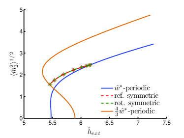
The symmetries of the pattern can be identified as linear representations of the dihedral group $D_{2N}$, where $N$ indicates the number of folds. The secondary bifurcation branches are computed with the help of a numerical branch switching algorithm which is adapted to the problem of multiple bifurcations. Generically, there are two distinct types of branches: Branches along which rotational symmetry is broken and reflectional symmetry is conserved and vice versa, see Figure 27. In case of the first type of branches, a fold collapses as two neighboring faces disappear; in case of the second type of branches, the number of folds decreases as one face disappears and the two adjacent faces merge. During the coarsening process, the width of the remaining folds is adjusted. Let us point out that the first instability of the $\hat{w}$-periodic concertina under $N\hat{w}$-periodic perturbations in the end leads to the collapse of exactly one fold – reducing the total number of folds from $N$ to $N-1$, see Figure 25.

Figure 27: Numerical simulations: Reflectional symmetric with respect to center wall (top) and rotational symmetric with respect to the midpoint of white face (bottom) magnetization pattern on the unstable bifurcation branch connecting the $\hat{w}^{*}$-periodic and the $\tfrac{4}{3}\hat{w}^{*}$-periodic branch. The central fold collapses (top); white face disappears and two adjacent black faces merge (bottom).

Figure 28: Experiment and numerical simulations: The coarsening of the concertina pattern in a Permalloy sample (top row) of $30$nm thickness and $70\upmu$m width compared to the numerical simulations (bottom row). A ripple-like structure grows into the concertina pattern. Within the numerical simulations we iteratively increment the external field and minimize the energy. The computational domain is of period $6\hat{w}^{*}$. The numerical images are scaled according to (9). The numerical image hence display 1.8 times the unit cell; the numerical images therefore appear to be more uniform than the experimental concertina.

III.6 Wavelength modulation in the experiments

In the experiments, the $x_{1}$-wavelength of the modulation is restricted by the finite extension of the sample. Moreover, inhomogeneities and defects of the material, in particular those at the edges of the cross section, strongly affect the formation. This is reflected by the fact that walls occur at the same pinning sites when the experiment is rerun. The existence of pinning sites hence leads to an effective modulation wavelength that is just a small multiple $N$ of the wavelength of the pattern. In particular we expect that pinning sites have a stabilizing effect and therefore prevent coarsening. Therefore, the seemingly artificial numerical simulation for small and moderate $N$, cf. Figure 25, may be more relevant for the experiment than the Bloch-wave analysis, i.e., $N\nearrow\infty$, cf. Section III.3.

III.7 Domain Theory: Instability for decreasing field

The experiments also show that the concertina period $\hat{w}$ decreases with decreasing external field $\hat{h}_{\text{ext}}$. This has a simple explanation on the level of domain theory, too. Suppose that the concertina period had increased at several coarsening events during the increase of the field. As the decreasing external field $\hat{h}_{\text{ext}}$ drops below its optimal scaling given the period $\hat{w}$, that is, for $\hat{w}\gg\hat{h}_{\text{ext}}\ln\hat{h}_{\text{ext}}$, the optimal concertina pattern does not suffer a long wavelength instability, but instead degenerates in the sense that the closure domains invade the whole cross section. Simulations of the reduced model confirm this scenario predicted by domain theory, see Figure 29, which shows a pattern of period $5\hat{w}^{*}$ close to the turning point: The numerical backward cycle, in which we start at the multiply coarsened state and then after minimization repeatedly decrease the external field by a fixed increment, shows that the coarsened pattern stays stable up to the turning point that coincides with the moment at which the pattern degenerates as mentioned above. Depending on the initial level of coarsening, the period is then either refined or we reach the uniformly magnetized state after the minimization.

Figure 29: Numerical simulations: The coarsened concertina pattern degenerates as the external field is reduced. The numerical simulations confirm the prediction based on domain theory: The pattern degenerates at the turning point of the branch.

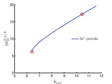
III.8 Conclusion: Hysteresis and scattering of data

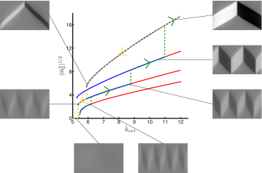
Summing up, domain theory in conjunction with a Bloch-wave argument indicates that the concertina pattern of period $w$ is present or stable at a given field $h_{\text{ext}}$ if and only if $w\sim\ell^{2}t^{-1}h_{\text{ext}}\ln(d^{-2/3}\ell^{4/3}t^{-2/3}h_{\text{ext}})$, which is confirmed by the numerical simulations. In particular we expect that the height of the triangular domains ($\sim\frac{w}{m_{2}^{0}}$) is close to constant as the external field increases, cf. (22) and (23). If the period deviates by a (large) factor from that expression, it becomes unstable. On the other hand, this analysis also suggest that there is a range of $w\sim\ell^{2}t^{-1}h_{\text{ext}}\ln d^{-2/3}\ell^{4/3}t^{-2/3}h_{\text{ext}}$ for which the concertina pattern is stable, see Figure 30. This may explain some of the scatter in the experimental data and the pattern’s hysteresis.

Figure 30: Numerical simulations: The marginally stable (red), optimal (blue) and maximal period (green) of the concertina pattern as a function of the external field $\hat{h}_{\text{ext}}$. The dashed and solid curves depict the result on the basis of the reduced model and on the basis of domain theory, respectively.

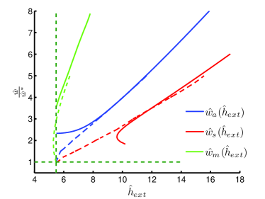
Figure 30 displays the marginally stable period (below the red curve the minimal energy per period is concave and thus the concertina of smaller period unstable as the field increases) and the optimal period depending on the external field. The upper green curve indicates the turning points of the $\hat{w}_{m}$-periodic branches, i.e., the smallest external field for which a concertina of a certain maximal period $\hat{w}_{m}$ exists – clearly the $m$ in $\hat{w}_{m}$ stands for maximal. Observe that the maximal period $\hat{w}_{m}$ on the basis of domain theory and on the basis of the reduced model coincide for large external field, too. The region bounded by $\hat{w}_{s}$ and $\hat{w}_{m}$ corresponds to the range of stable periods.

Figure 31: Numerical simulations: The hysteresis loop. As we increase the external field we follow the red path: The concertina pattern coarsens if the period is smaller than the stable period. As we decrease the field we follow the yellow path: Starting from a coarsened concertina the pattern degenerates as we reach the turning point of the branch. The pattern refines towards the optimal period until it finally disappears.

Figure 32: Experiment: The hysteresis cycles of a Permalloy sample of $30$nm thickness and $50\upmu$m width. The upper row shows the pattern as the external field increases (from left to right), the lower row shows the pattern as the external field decreases (from right to left).

IV Discretization and numerical simulations

The numerical simulations are based on a finite difference discretization of the reduced rescaled energy functional (12). The transversal component $\hat{m}_{2}$ is approximated on a uniform Cartesian grid. The discretization of the exchange, anisotropy and Zeeman energy is straight forward. In case of the non-linear charge density $\hat{\sigma}=-\hat{\partial}_{1}\frac{\hat{m}_{2}^{2}}{2}+\hat{\partial}_{2}\hat{m}_{2}$ our choice of a finite difference stencil is motivated by the inheritance of the shear invariance (17). The stray-field energy can efficiently be computed using Fast Fourier Transform with respect to $\hat{x}_{1}$. For an introduction of the discretization scheme see [18, Subsection 3.2]. Note that the computation of the energy and related quantities, such as gradient or Hessian, can be parallelized since the non-locality is only with respect to one dimension. For the parallelization we decompose the computational domain into horizontal slices with respect to $\hat{x}_{2}$.

Figure 33: Tangent predictor-corrector continuation method.

We apply numerical simulations to compute (local) minimizers and stationary points. The naive approach using steepest descent algorithms for the computation of minimizers is slow and even fails close to bifurcation points. The iterative path-following techniques that we apply in order to compute an approximation to a branch of stationary points are adapted to such situations, cf. [11]. The local tangent $t^{n}$ in a stationary point $(\hat{m}^{n},\hat{h}_{\text{ext}}^{n})$ of the branch is used to obtain a predictor for the next point on the branch $(m_{2}^{n+1},h_{\text{ext}}^{n+1})$, cf. Figure 33. Within the corrector step the predictor is orthogonally (to the tangent) projected onto the branch. This step amounts to the solution of a non-linear equation, more precisely an augmented Euler-Lagrange equation:

$$\left(\begin{array}[]{c}\nabla_{\hat{m}_{2}}\hat{E}(\hat{m}^{n+1}_{2},\hat{h}^{n+1}_{\text{ext}})\\ ((\hat{m}^{n+1}_{2},\hat{h}^{n+1}_{\text{ext}})-p^{n+t})\cdot t^{n}\end{array}\right)=0.$$

A bifurcation point can be detected with the help of an appropriate indicator function, cf. [11]. However, both the bifurcation detection and the branch-switching technique which are described in that reference are applicable for simple bifurcations points only. As described in detail in [19], both methods can be modified in order to cope with multiple bifurcation points. This extension relies on the fact that multiple bifurcations which occur due to symmetries of the primary solution generically can be reduced to simple bifurcation points, cf. [12].

V Polycrystalline anisotropy

The experiments usually do not show a clear-cut critical field with a first-order transition (i.e., subcritical bifurcation). This can be due to lack of experimental resolution (the amplitude of the transversal component $\langle m_{2}^{2}\rangle^{1/2}=d^{2/3}\ell^{-1/3}t^{-1/3}\langle\hat{m}_{2}^{2}\rangle^{1/2}$ at the turning point ranges between $0.015$ to $0.063$ for typical sample dimensions, namely widths $\ell$ between $10$ to $50\upmu$m and thicknesses $t$ between $30$ and $100$nm) or due to the presence of the so-called ripple that smoothes out the transition, as we shall explain in this section. The ripple is the in-plane small-scale oscillation of the magnetization – perpendicular to its average direction – in extended films. In this section, we show how the linear ripple theory developed in [14, 13] can be incorporated into our theory for the concertina – and explains the smoothing-out of the first-order transition encountered in Section I.9.

The ripple is triggered by an effective field of random direction on a small scale. Several origins for this effective field have been proposed in the literature, see for instance [13, Section C]; in polycrystalline thin films, the random orientation of the grains (via crystalline anisotropy) and local stresses (via magnetostriction) are seen as the main causes. In our discussion, we focus on the former.

Hoffmann [14] and Harte [13], based on the torque equilibrium, linearized around a spatially constant magnetization (solely determined by the external field and anisotropy). Hereby they identified the linear response to (for instance) such a small-scale, small-amplitude random effective field. The main finding is that the stray field – which penalizes transversal more than longitudinal perturbations of the magnetization because the former lead to a stronger charge oscillation – results in a strong anisotropy of the response. Hoffmann [14] characterized this response in terms of the Green’s function, whereas Harte [13] characterized it in terms of the multiplier in Fourier space, i.e., $k$-space. Since Hoffmann chose to expand the Green’s function (in a self-consistent way on the level of the length scale) in terms of a Bessel function, see [14, (5)], it deviates order one from the exact expression in [16, 2].

Clearly, the anisotropic rescaling (9) leading to our reduced model and the anisotropic response have the same origin. We will see that both the ripple and the transition between ripple and concertina can be explained within the framework of an extension of our reduced model. We note that our analysis of the ripple is mainly a reformulation of the classical results. However, the new insight is that the finite width $\ell$ of the sample leads to a (continuous) transition from the ripple to the concertina.

We now explain how to extend our reduced model. We start from the 3-d model (1) with a uniaxial anisotropy of strength $Q$ and position-dependent easy axis $e(x)$, i.e., with the term $-Q\int(m\cdot e)^{2}\operatorname{d}\!x$. In the approximation of our reduced model, i.e., $m_{3}\equiv 0$, $m=m(x_{1},x_{2})$, and the linearization $m_{1}\approx 1-\frac{m_{2}^{2}}{2}$ due to $m_{2}^{2}\ll 1$, this term is, up to additive constants, to leading order approximated by $-2Qt\int m_{2}\overline{e_{1}e_{2}}\operatorname{d}\!x_{1}\operatorname{d}\!x_{2}$, where $\overline{e_{1}e_{2}}(x_{1},x_{2})$ denotes the vertical average of the product of the first two components of the easy axis $e=(e_{1},e_{2},e_{3})$. A random anisotropy therefore acts to leading order as a random transversal external field

$$-2t\int_{\Omega^{\prime}}h_{\text{ripple}}m_{2}\operatorname{d}\!x_{1}\operatorname{d}\!x_{2},$$ (27)

where $h_{\text{ripple}}=Q\overline{e_{1}e_{2}}$. As mentioned, the position dependence of $e$ arises from the random orientation of the grains of size $\ell_{grain}$. Provided $t\ll\ell_{grain}\ll w^{*}$ (where we take $w^{*}$ as a typical length scale of the magnetization pattern), the stationary statistics of $\overline{e_{1}e_{2}}$ are characterized by

$$\langle\overline{e_{1}e_{2}}(0,0)\overline{e_{1}e_{2}}(x_{1},x_{2})\rangle\\ =\ell_{grain}^{2}\delta(x_{1})\delta(x_{2})\langle\overline{e_{1}e_{2}}(0,0)^{2}\rangle,$$ (28)

where $\langle\cdot\rangle$ denotes the ensemble average and $\delta$ the Dirac function.

For subcritical fields $h_{\text{ext}}<h_{\text{ext}}^{*}$, we neglect the non-linear term in the stray-field energy in (7). The resulting energy functional is quadratic and linear in $m_{2}$, hence it is conveniently expressed in terms of ${\mathcal{F}}m_{2}(k_{1},k_{2})$, which denotes the Fourier transform of $m_{2}$ in $x_{1}$ and the Fourier sine series in $x_{2}$:

$$E(m_{2})\\ \approx\int_{-\infty}^{\infty}\sum_{k_{2}\in\frac{\pi\mathbb{Z}}{\ell}}(d^{2}k_{1}^{2}+\tfrac{1}{2}tk_{2}^{2}k_{1}^{-1}-h_{\text{ext}})|\mathcal{F}m_{2}|^{2}\\ -2\mathcal{F}h_{\text{ripple}}\mathcal{F}^{-1}m_{2}\operatorname{d}\!k_{1}.$$

The explicit minimization yields

$${\mathcal{F}}m_{2}(k_{1},k_{2})=\tfrac{1}{(d^{2}k_{1}^{2}+\tfrac{1}{2}tk_{2}^{2}k_{1}^{-1}-h_{\text{ext}})}{\mathcal{F}}h_{\text{ripple}}(k_{1},k_{2}).$$ (29)

We interpret this $m_{2}$ as the ripple. Since (28) on the level of ${\mathcal{F}}\overline{e_{1}e_{2}}$ reads $\langle|{\mathcal{F}}\overline{e_{1}e_{2}}(k_{1},k_{2})|^{2}\rangle=\ell^{2}_{\text{grain}}$, (29) is best expressed in terms of the energy spectrum:

$$\langle|{\mathcal{F}}m_{2}(k_{1},k_{2})|^{2}\rangle=Q^{2}\tfrac{\ell^{2}_{\text{grain}}}{(d^{2}k_{1}^{2}+\tfrac{1}{2}tk_{2}^{2}k_{1}^{-1}-h_{\text{ext}})^{2}}.$$ (30)

This formula clearly displays the afore mentioned anisotropic response of $m_{2}$ to the isotropic field $h_{\text{ripple}}$.

From formula (30) one can infer the predominant wavenumber of the ripple, that is,

$$\langle|k_{1}|\rangle=\frac{\sum_{k_{2}}\int_{-\infty}^{\infty}|k_{1}|\langle|\mathcal{F}m_{2}|^{2}\rangle\operatorname{d}\!k_{1}}{\sum_{k_{2}}\int_{-\infty}^{\infty}\langle|\mathcal{F}m_{2}|^{2}\rangle\operatorname{d}\!k_{1}}.$$ (31)

For moderate stabilizing fields $t^{2}d^{-2}\gg-h_{\text{ext}}\gg d^{-2/3}\ell^{4/3}t^{-2/3}$, we obtain from (31) that the average wavenumber scales as $\langle|k_{1}|\rangle\sim(-h_{\text{ext}})^{1/2}d^{-1}\ll td^{-2}$. This is the scaling of the predominant wavenumber of the ripple in an extended film [14, p.34, (7)]. Notice that the lower bound characterizing Regime III is equivalent to $t^{2}d^{-2}\gg d^{-2/3}\ell^{4/3}t^{-2/3}$. For large stabilizing fields $-h_{\text{ext}}\gg t^{2}d^{-2}$ one can show that the average amplitude of the ripple, given by $\int\sum_{k_{2}}\langle|\mathcal{F}m_{2}|^{2}\rangle\operatorname{d}\!k_{1}$, tends to zero. Moreover, from (31), because of the discreteness of $k_{2}$, we can infer

$$\lim_{h_{\text{ext}}\uparrow h_{\text{ext}}^{*}}\langle|k_{1}|\rangle=\frac{2\pi}{w^{*}},$$

which is the wavenumber of the unstable mode (6). We thus learn that, as the strength $h_{\text{ext}}$ of the external field increases from negative values towards the critical value, the average wavelength of the ripple continuously increases

• from the values characteristic for a film which is infinite in both $x_{1}$ and $x_{2}$-directions

• to the wavelength of the unstable mode that is at the origin of the concertina pattern (which depends on the sample width).

Due to this transition it is thus not surprising that ripple and small-amplitude concertina are difficult to distinguish.

We now address the numerical simulation of our augmented model (32). Let us therefore first rewrite the additional term (27) in the rescaled variables (9). The rescaled reduced model (12) is augmented by

$$-2\int\hat{h}_{\text{ripple}}\hat{m}_{2}\operatorname{d}\!\hat{x}_{1}\operatorname{d}\!\hat{x}_{2},$$ (32)

where $\hat{h}_{\text{ripple}}$ is a stationary Gaussian field of vanishing mean and of variance

$$\langle\hat{h}_{\text{ripple}}(0,0)\hat{h}_{\text{ripple}}(\hat{x}_{1},\hat{x}_{2})\rangle=(\sigma^{*})^{2}\delta(\hat{x}_{1})\delta(\hat{x}_{2}),$$ (33)

with $\sigma^{*}=d^{-10/6}\ell^{5/6}t^{-1/6}Q\ell_{grain}\langle\overline{e_{1}e_{2}}(0,0)^{2}\rangle^{1/2}$. In case of a uniform distribution of the anisotropy axis in the plane, we have for example that $\langle\overline{e_{1}e_{2}}(0,0)^{2}\rangle=\frac{1}{8}.$

On the level of the discretization, the field $\hat{h}_{\text{ripple}}$ is modeled as a Gaussian random variable of mean zero, which is identically and independently distributed from grid point to grid point and has variance $(\sigma^{*})^{2}{\Delta\hat{x}_{1}}^{-1}{\Delta\hat{x}_{2}}^{-1}$, where $\Delta\hat{x}_{i}$ denotes the grid size in direction $\hat{x}_{i}$. For the numerical simulations we thus have to determine the value of $\sigma^{*}$ for a typical sample. Let us consider a film of $30$nm thickness and $70\upmu$m width with typical grain size $\ell_{\text{grain}}=15nm$. For a local strength of anisotropy $Q=5\times 10^{-3}$ we obtain that $(\sigma^{*})^{2}=125.87$. For the value of $(\sigma^{*})^{2}=110.83$, our numerical simulation indeed shows a continuous transition from the ripple to the concertina pattern instead of a first-order phase transition due to a subcritical bifurcation, see Figure 28.

We also believe that our reduced model is the appropriate framework to analyze the non-linear corrections to the linear ripple theory. Indeed, we have seen in Section I.9 that it captures the transition from the unstable mode to low-angle symmetric Néel walls. We thus believe it also captures the transition from the ripple to the blocked state that is related to hysteresis in extended thin films [10].

Closing this section, we contrast the ripple, that can be seen as a consequence of quenched disorder, to the effects of thermal fluctuations. Thermal fluctuations can be modeled by a random external field term in the Landau-Lifschitz-Gilbert equation that is white noise in space and time. The reason for modeling thermal fluctuations by a space-time white noise torque in the Landau-Lifschitz-Gilbert equation is that the stationary measure of this Langevin equation is given by the Gibbs distribution

$$\frac{1}{Z}\exp(-E(m))\operatorname{d}\!m,$$ (34)

where $E(m)$ is the 3-d micromagnetic energy functional and $\operatorname{d}\!m$ is best thought of as the high, but finite-dimensional measure after spatial discretization of $m$. Following [1, Subsection 2.4], we consider a situation where the constant magnetization, say $m=(1,0,0)$, is a strict global minimizer of $E$ (because of a sufficiently strong external field in direction $(1,0,0)$). This justifies to replace $E(m)$ and $\operatorname{d}\!m$ in (34) by its Hessian ${\rm Hess}(\delta m,\delta m)$ in $(1,0,0)$ and $\operatorname{d}\!\delta m_{2}\operatorname{d}\!\delta m_{3}$, respectively. This has the advantage that we obtain a Gaussian measure that can be explicitly analyzed. The outcome is the following: In case of a bulk material, the expected value of $\delta m_{2}^{2}+\delta m_{3}^{2}$ diverges as the mesh size $\Delta x$ goes to zero; the expected value of the wavenumber $|k|$ behaves as $\Delta x^{-1}$. The same holds for thin films, although the divergence is just logarithmic.

This simple analysis highlights the need of a renormalization in case of thermal fluctuations. As we have seen, quenched disorder coming from polycrystallinity can be modeled by a random field term in the micromagnetic energy that is white noise only in space. As opposed to thermal fluctuations, there is no divergence in the amplitude of the excitations in case of such a field term that is white noise in space only – the critical dimension for this random effect is four. Moreover, in thin films, the dominant wavelength of the in-plane fluctuations excited by such a field is determined by both exchange and stray-field energy and turns out to be much larger than the atomistic length scale $d$ and the typical grain size $\ell_{\text{grain}}$.

VI Uniaxial anisotropy

We now address the effect of uniaxial anisotropy – constant throughout the sample – on the formation of the concertina pattern. We focus on the two cases in which the easy axis coincides with the $x_{2}$-axis (transversal anisotropy $e=(0,1,0)$ in (1)) or in which the easy axis coincides with the $x_{1}$-axis (longitudinal anisotropy $e=(1,0,0)$ in (1)). Clearly, such type of anisotropy has no effect on the stationary point of the energy, i.e., the uniform magnetization. On the level of the reduced model both cases can be represented (up to an additive constant) by the additional quadratic term

$$-Q\;t\int m_{2}^{2}\,\operatorname{d}\!x_{1}\operatorname{d}\!x_{2}$$ (35)

with a signed quality factor $Q$. Transversal anisotropy corresponds to $Q>0$, longitudinal anisotropy corresponds to $Q<0$.

As will become clear below, when considering the effects of anisotropy, it is appropriate to expand the Zeeman term to quartic order, i.e.,

$$-h_{\text{ext}}\;t\int(m_{2}^{2}+\tfrac{m_{2}^{4}}{4}\,)\operatorname{d}\!x_{1}\operatorname{d}\!x_{2}.$$

The following Gedankenexperiment is helpful in understanding the sequel: In extended thin films, i.e., $\ell=\infty$, there is no incentive for a spatially varying magnetization so that we may consider a constant magnetization $m_{2}$ in which case the relevant energy per volume is given by $-Qm_{2}^{2}-h_{\text{ext}}(m_{2}^{2}+\frac{m_{2}^{4}}{4})$. In this case the critical field is given by $h_{\text{ext}}^{*}=-Q$. For longitudinal anisotropy, the bifurcation is subcritical, whereas for transversal anisotropy, the bifurcation is supercritical and yields

$$m_{2}=\pm(2(1+Q^{-1}h_{\text{ext}}))^{1/2}.$$ (36)

Hence for finite $\ell$, there are two competing mechanisms which lead to a bifurcation and a selection of an amplitude for $m_{2}$: uniaxial anisotropy and shape anisotropy in form of the stray-field energy.

As we will see in the sequel, there are essentially three different effects of anisotropy: a linear one, a weakly non-linear one, and a strongly non-linear one, which we list and characterize below. Notice that the order at which these effects arise with increasing anisotropy does not agree with their ordering with increasing non-linearity, cf. Figure 34: The linear effect becomes pronounced for $|Q|\gg d^{2/3}\ell^{-4/3}t^{2/3}$, the strongly non-linear one for $|Q|\gg\ell^{-1}t$, and the weakly non-linear one only for $|Q|\gg d^{-2/3}\ell^{-2/3}t^{4/3}$. Note that we have that $d^{2/3}\ell^{-4/3}t^{2/3}\ll\ell^{-1}t\ll d^{-2/3}\ell^{-2/3}t^{4/3}$ provided $d^{2}\ell^{-1}\ll t$, which is the lower bound on the film thickness which characterizes Regime III.

Figure 34: The order of the different effects of anisotropy

We mainly focus on the case of transversal anisotropy $Q>0$. In case of longitudinal anisotropy $Q<0$ we give an explanation for the experimental fact that the concertina cannot be observed at all.

Linear effect for weak anisotropy

$|Q|\gg d^{2/3}\ell^{-4/3}t^{2/3}$. An obvious effect of anisotropy is a shift of the critical field $h_{\text{ext}}^{*}$ by the amount $-Q$; we call it the “linear effect” of anisotropy since it arises on the level of the linearization at $m_{2}\equiv 0$. In view of the scaling of the critical field $h_{\text{ext}}^{*}$ at $Q=0$, i.e., (10), we infer that the value of the critical field is dominated by the uniaxial anisotropy, i.e.,

$$h_{\text{ext}}^{*}\approx-Q\quad\text{for}\quad|Q|\gg d^{2/3}\ell^{-4/3}t^{2/3}.$$ (37)

We note that a transversal anisotropy decreases the distance between the two critical fields $\pm h_{\text{ext}}^{*}$ corresponding to the stationary states $\pm m^{*}$; in particular, for $Q\sim d^{2/3}\ell^{-4/3}t^{2/3}$, the critical field changes sign and thus the order between the two critical fields switches. (Likewise for longitudinal anisotropy the distance decreases.) Although a clear-cut critical field cannot be observed in the experiments due to the polycrystalline structure which triggers the ripple, and since the value of the effective external field at the investigated sample section is not available, the linear effect could be qualitatively confirmed: For Permalloy samples of high (transversal) anisotropy the oscillatory instability occurs before the external field is reversed. In accordance with (37), we observe for relatively wide films that the relative strength of anisotropy increases and the critical field decreases (theoretically approaching $-Q$). On the other hand for low-anisotropic Permalloy the first oscillation is observed close to zero external field.

Weakly non-linear effect

for strong anisotropy $|Q|\gg t(w^{*})^{-1}\sim d^{-2/3}\ell^{-2/3}t^{4/3}$. For sufficiently strong anisotropy $Q$, the quartic term coming from the stray-field energy no longer dominates the quartic term coming from the Zeeman energy near the bifurcation. We call this effect the “weakly non-linear effect” of anisotropy, since it can be analyzed on the level of an expansion of the reduced energy near $m_{2}\equiv 0$ and $h_{\text{ext}}=h_{\text{ext}}^{*}$, cf. (14), where we take into account the quartic Zeeman term $-\frac{h_{\text{ext}}}{4}tA^{4}\int(m_{2}^{*})^{4}\operatorname{d}\!x_{1}\operatorname{d}\!x_{2}$. The shift of the critical field suggests the following rescaling for the reduced external field

$$\hat{h}_{\text{ext}}=d^{-2/3}\ell^{4/3}t^{-2/3}(h_{\text{ext}}+Q).$$

In addition we set

$$\hat{Q}=-\tfrac{1}{4}d^{2/3}\ell^{2/3}t^{-4/3}h_{\text{ext}}$$

so that we obtain with the same rescaling of energy, length and magnetization as in (9) and (11) the reduced energy functional augmented by

$$+\hat{Q}\int_{\hat{\Omega}^{\prime}}\hat{m}_{2}^{4}d\hat{x}_{1}d\hat{x}_{2}.$$

Therefore the energy close to the bifurcation takes the form of

$$\hat{E} (A\hat{m}_{2}^{*}+A^{2}\hat{m}_{2}^{**})$$

$$\approx-(\tfrac{\pi}{2})^{1/3}(\hat{h}_{\text{ext}}-\hat{h}_{\text{ext}}^{*})\,A^{2}+(\tfrac{9}{64}\hat{Q}-\tfrac{\pi}{640})A^{4}.$$

For $|Q|\gg d^{-2/3}\ell^{-2/3}t^{4/3}\gg d^{2/3}\ell^{-4/3}t^{2/3}$ the critical field asymptotically behaves as $h_{\text{ext}}^{*}\approx-Q$, cf. (37), so that the reduced quality factor behaves as $\hat{Q}\approx\frac{1}{4}d^{2/3}\ell^{2/3}t^{-4/3}\,Q$ close to the critical field. From the latter we read off that in the regime $Q\gg d^{-2/3}\ell^{-2/3}t^{4/3}$ the quartic coefficient becomes positive and therefore the bifurcation becomes supercritical, cf. Figure 35. Essentially it is a perturbation of the constant-magnetization bifurcation in infinitely extended films mentioned above, cf. (36). In particular, the selected amplitude in this case scales as $m_{2}\sim A\sim(1+h_{\text{ext}}Q^{-1})^{1/2}$. On the level of the extended bifurcation analysis one finds that the period of the unstable mode $w^{*}$ lies in the stable region in the neighborhood of the critical field. In agreement with this, for increasing external fields the numerical simulations show that no modulation instability occurs and that there is no coarsening. We note that domain theory is consistent with the numerical simulations, too.

Figure 35: Numerical simulations: Transition from sub- to supercritical bifurcation as strength of transversal anisotropy increases. For $Q=0.03\approx Q^{*}$ the bifurcation degenerates.

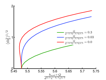
On the other hand, for large longitudinal anisotropy, i.e., $-Q\gg d^{-2/3}\ell^{-2/3}t^{4/3}$, we expect that there is no turning point on the bifurcating branch so that it remains unstable – to the effect that no concertina pattern forms in the first place. The numerical simulations in Figure 36 show a second turning point which coincides with the break-up of the concertina pattern. For even larger longitudinal anisotropy the first turning point is destroyed, cf. Figure 36.

Figure 36: Numerical simulations: Loss of the turning point as strength of longitudinal anisotropy increases

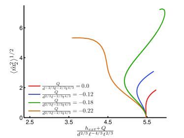
This observation can also be confirmed on the level of domain theory where we take into account anisotropy and the quartic term in the Zeeman energy, cf. (21):

$$e_{\text{domain}}(m_{2}^{0},w)\,=\, 2\left(\ell-\tfrac{w}{m_{2}^{0}}\right)e(m_{2}^{0})+4\,\frac{w}{m_{2}^{0}}\,e\left(\tfrac{m_{2}^{0}}{2}\right)$$

$$-(h_{\text{ext}}+Q)(m_{2}^{0})^{2}t\left(w\ell-\tfrac{w^{2}}{m_{2}^{0}}\right)$$

$$-h_{\text{ext}}\tfrac{1}{4}(m_{2}^{0})^{4}t\left(w\ell-\tfrac{w^{2}}{m_{2}^{0}}\right).$$ (38)

The quartic wall energy cannot compensate the destabilizing quartic Zeeman contribution provided $h_{\text{ext}}\,t\,w\gg\,t^{2}$ (up to a logarithm). Therefore due to $h_{\text{ext}}^{*}\sim-Q$ and $w\sim d^{2/3}\ell^{2/3}t^{-1/3}$ close to the bifurcation there are no (local) minimizers of the energy.

Typical values for our Permalloy samples of strong uniaxial anisotropy range from $\hat{Q}=\frac{|Q|}{4d^{-2/3}\ell^{-2/3}t^{4/3}}\approx 2.1\times 10^{-4}$ to $0.023$ depending on the sample’s width and thickness ($Q=5\times 10^{-4}$, $t=10$nm to $150$nm, $\ell=10\upmu$m to $50\upmu$m). Typical values for CoFeB range from $\hat{Q}=7.8\times\times 10^{-4}$ to $0.011$ ($Q\approx 1.5\times 10^{-3}$, $t=30$nm-$100$nm, $\ell=10\upmu$m-$50\upmu$m). The uniaxial anisotropy is thus too small to cause the weakly non-linear effect. However, although local minimizers of the energy might exist in case of longitudinal anisotropy, still the energy is not coercive as soon as the external field is reversed.

Strongly non-linear effects

for moderate anisotropy $|Q|\gg\ell^{-1}t$. In that case one can distinguish two different scenarios in the formation of the concertina:

• Scenario I: If the amplitude (and shape) of the concertina pattern would not be affected by anisotropy (besides the critical field at which it bifurcates), like in an infinitely extended film, its optimal amplitude would scale as

  $${m_{2}}_{a}\sim\ell t^{-1}(h_{\text{ext}}-h_{\text{ext}}^{*}) \overset{\eqref{smallaniso}}{\approx}\ell t^{-1}(h_{\text{ext}}+Q)$$

  $$=\ell t^{-1}Q(1+Q^{-1}h_{\text{ext}}),$$ (39)

  up to a logarithm for $h_{\text{ext}}-h_{\text{ext}}^{*}\gg d^{2/3}\ell^{-4/3}t^{2/3}$, as we have seen in (23) in Section III.1.

• Scenario II: If the amplitude of the concertina pattern would be dominated by transversal anisotropy, it would behave as

  $${m_{2}}_{a}\overset{\eqref{predaniso2}}{\sim}(1+Q^{-1}h_{\text{ext}})^{1/2}$$ (40)

  for $0<(1+Q^{-1}h_{\text{ext}})\ll 1$.

Hence we expect that for $Q\gg\ell^{-1}t$, the concertina pattern is limited by stray field effects as long as $0<1+Q^{-1}h_{\text{ext}}\ll(Q^{-1}\ell^{-1}t)^{2}$ and by anisotropy effects once $(Q^{-1}\ell^{-1}t)^{2}\ll 1+Q^{-1}h_{\text{ext}}\ll 1$. Loosely speaking, the effect of anisotropy kicks in for a large amplitude and is most prominent close to field strength where the concertina pattern vanishes. We call this the “strongly non-linear effect” of anisotropy. (Also this provides a reason to expand the Zeeman term to higher order.)

We note that we have to take into account the lower order wall energy in Scenario II in order to determine the optimal period. In that case, a minimization of the energy per length yields the following scaling behavior of the optimal period (up to a logarithm)

$$w_{a}\sim(\ell t)^{1/2}Q^{-1/2}(1+Q^{-1}h_{\text{ext}})^{1/4}.$$

As we know from Section III the experimentally more relevant quantity is the marginally stable period, i.e., the largest period (as a function of the external field) for which the minimal energy is convex. At the cross-over we expect that the marginally stable period is of the order $\sim tQ^{-1}$, cf. Figure 39. In fact, due to $(Q^{-1}\ell^{-1}t)^{2}\sim 1+Q^{-1}h_{\text{ext}}$ at the cross-over, we have that $w\sim\ell^{2}t^{-1}Q(1+Q^{-1}h_{\text{ext}})\sim tQ^{-1}$, see (39) together with the fact that $w_{s}\sim\ell{m_{2}}_{a}$. For a period of that order the minimal energy in Scenario II turns out to be convex. Hence we expect that the coarsening stops once $(Q^{-1}\ell^{-1}t)^{2}\ll 1+Q^{-1}h_{\text{ext}}\ll 1$. Still the transversal component of the magnetization grows as $m_{2}\sim(1+Q^{-1}h_{\text{ext}})^{1/2}$ so that size and height of the closure domains decrease.

Figure 37: Experiment: Permalloy samples of width $60\upmu$m to $150\upmu$m of high anisotropy and at the end of the coarsening process. The $6$ samples on the right are of thickness $30$nm, the $6$ samples on the right are of thickness $50$nm. The period of the pattern appears to be independent of the width of the samples, in agreement with our theoretical prediction as an effect of anisotropy.

Figure 39 displays the transition of the scaling behavior in the optimal period, the marginally stable period, and the amplitude of the transversal magnetization component. At the cross-over we have that $m_{2}\sim t(\ell Q)^{-1}\ll 1$ and $w\sim tQ^{-1}\ll\ell$. This is consistent with the assumptions of the reduced model, i.e., the low-angle approximation and the scale separation of the dominant length scales with respect to $x_{1}$ and $x_{2}$. For the same reason and due to the observation that $h_{\text{ext}}+Q\gg d^{2/3}\ell^{-4/3}t^{2/3}$ implies $\hat{h}_{\text{ext}}\gg 1$, also (low-angle) domain theory is applicable up to the cross-over to Scenario II. (As $m_{2}$ tends towards one in Scenario II solely domain theory is applicable, the low-angle approximation has to be dropped – in particular for the wall energy.)

Let us mention another observation supporting the conjecture that anisotropy effects are most prominent close to the field strength where the concertina vanishes: For $Q\gg\ell^{-1}t$, the ground state for vanishing external field $h_{\text{ext}}=0$ is no longer given by the uniform magnetization $m=(\pm 1,0,0)$, but a Landau or Concertina-type pattern, see Figure 38, has lower energy. The optimal periods $w$ of the two latter pattern are determined by a balance of the wall energy and the anisotropy energy in the closure domains, and scale as $w\sim Q^{-1/2}(\ell t)^{1/2}$ up to a logarithm. Hence we expect that in this regime, the concertina does not switch to $m=(-1,0,0)$, but evolves to the pattern in Figure 38.

Figure 38: Continuous transition from the concertina pattern via the Landau state to the reversed concertina. Note that the total length of the walls and the Zeeman energy do not change while the anisotropy energy is smaller in case of the Landau state.

In fact, that type of transition of the concertina pattern can be observed in CoFeB samples – that posses a stronger (transversal) uniaxial anisotropy, cf. Figure 40.

Figure 39: Table of scaling behavior of the optimal and marginally stable period and the amplitude of the transversal component in the regime $t\ell^{-1}\ll Q\ll d^{-2/3}\ell^{-2/3}t^{4/3}$.

Figure 40: Experiment: Hysteresis of a CoFeB sample of $60$nm thickness and $30\upmu$m width. Following the coarsening we observe a transition to a Landau state at $0$ external field which turns into a concertina which degenerates and refines, and finally disappears.

VII Conclusion

In this work, we addressed the concertina pattern in very elongated thin-film elements. We provided an explanation of the formation and the coarsening of this pattern as the external field is reduced from saturation.

We identified a parameter regime in which the uniform magnetization becomes unstable to an oscillatory buckling mode. In this parameter regime, we derived a two-dimensional and thus numerically tractable reduced energy functional from three-dimensional micromagnetics. On the basis of the reduced model, we performed numerical bifurcation analysis: The bifurcation is slightly subcritical, but has a turning point, after which the buckling mode grows into the concertina pattern with its low-angle Néel walls. This is an alternative explanation for the formation of the concertina to the one proposed by van den Berg: An outgrow of an unstable mode instead of an in-grow of closure domains. Over a wide range of sample sizes, there is a good agreement between the explicit period of the unstable mode and the measured average period of the concertina pattern. In particular, the predicted dependence on film thickness and width is confirmed. However, the measured period exceeds the theoretically predicted one by a factor up to approximately two.

We gave an argument for this initial deviation that at the same time explains the coarsening: Domain theory based on the reduced model – where low-angle Néel walls are replaced by sharp discontinuity lines – shows that coarsened configurations are energetically favorable. More importantly, uncoarsened configurations eventually become unstable because the energy per period becomes concave. Based on the reduced model, we argued by a Bloch-wave Ansatz that this concavity indeed translates into a secondary instability of the concertina pattern with respect to long wave-length modulations. These secondary instabilities are confirmed by numerical bifurcation analysis. The long wave-length instabilities are further confirmed by an extended bifurcation analysis that capitalizes on the near-degeneracy of the primary bifurcation. This extended bifurcation analysis also showed that that the long wave-length instability of the primary branch extends all the way down to the turning point. Hence at the moment of its appearance, the concertina pattern already has a resulting period larger than the one of the unstable mode. That qualitatively explains the deviation between the period of the unstable mode and the measured period of the concertina. Incidentally, these secondary instabilities are an asymmetric (with respect to the wave number) version of the Eckhaus instability introduced in the context of convective problems.

We gave yet another argument for the deviation of the period of the unstable mode from the measured period of the concertina at its formation. Based on the reduced model, we established a continuous transition from the magnetization ripple, which is triggered by the polycrystalline structure of the material, and the concertina pattern. On the level of the reduced model, the effect of an easy axis that varies from grain to grain translates into a random transversal external field that smears out the subcritical bifurcation. Hence for a sufficiently strong ripple effect, as the concertina pattern becomes discernible from the ripple, it has already coarsened.

Finally, we investigated the effects of a weak uniaxial material anisotropy on the concertina pattern. We distinguished three effects: 1) a shift of the critical field that changes its sign already for weak anisotropies, 2) a change in the coarsened concertina pattern from “limited by shape anisotropy” to “limited by material anisotropy” that kicks in for somewhat larger anisotropies, 3) a change from a subcritical to a supercritical bifurcation for a sufficiently large transversal anisotropy.

The various analyses render a fairly complete picture of the energy landscape that in particular explains the hysteresis of the concertina pattern.

VIII Acknowledgment

JM, RS, and HW thank R. Mattheis and R. Kaltofen for help with the thin-film deposition. FO and JS thank Alexander Mielke for helpful discussions on the Eckhaus instability and Martin Zimmermann for technical support.

References

- BG [05] D. V. Berkov and N. L. Gorn. Stochastic dynamic simulations of fast remagnetization processes: recent advances and applications. Journal of Magnetism and Magnetic Materials”, 290-291(Part 1):442 – 448, 2005. Proceedings of the Joint European Magnetic Symposia (JEMS’ 04).
- Bro [70] W. Brown. A critical assessment of Hoffmann’s linear theory of ripple. IEEE Transactions on Magnetics, 6:121–129, March 1970.
- BS [89] P. Bryant and H. Suhl. Thin-film magnetic patterns in an external field. Applied Physics Letters, 54(22):2224–2226, 1989.
- [4] R. Cantero-Álvarez and F. Otto. Critical fields in ferromagnetic thin films: identification of four regimes. J. Nonlinear Sci., 16(4):351–383, 2006.
- [5] R. Cantero-Álvarez and F. Otto. Oscillatory buckling mode in thin-film nucleation. J. Nonlinear Sci., 16(4):385–413, 2006.
- CÁOS [07] R. Cantero-Álvarez, F. Otto, and J. Steiner. The concertina pattern: a bifurcation in ferromagnetic thin films. J. Nonlinear Sci., 17(3):221–281, 2007.
- DKM+ [01] A. DeSimone, R. V. Kohn, S. Müller, F. Otto, and R. Schäfer. Two-dimensional modelling of soft ferromagnetic films. R. Soc. Lond. Proc. Ser. A Math. Phys. Eng. Sci., 457(2016):2983–2991, 2001.
- DKMO [05] A. DeSimone, R. V. Kohn, S. Müller, and F. Otto. Recent analytical developments in micromagnetics. In Giorgio Bertotti and Isaak Mayergoyz, editors, The Science of Hysteresis, volume 2, chapter 4, pages 269–381. Elsevier Academic Press, 2005.
- Eck [92] W. Eckhaus. On modulation equations of the Ginzburg-Landau type. In ICIAM 91 (Washington, DC, 1991), pages 83–98. SIAM, Philadelphia, PA, 1992.
- Fel [61] Ernst Feldtkeller. Blockierte drehprozesse in dünnen magnetischen schichten. Elektronische Rechenanlagen, 3(4):167–175, 1961.
- Geo [01] K. Georg. Matrix-free numerical continuation and bifurcation. Numer. Funct. Anal. Optim., 22 (3-4):303–320, 2001.
- GS [02] M. Golubitsky and I. Stewart. The symmetry perspective, volume 200 of Progress in Mathematics. Birkhäuser Verlag, Basel, 2002. From equilibrium to chaos in phase space and physical space.
- Har [68] K. J. Harte. Theory of magnetization ripple in ferromagnetic films. Journal of Applied Physics, 39(3):1503 –1524, 1968.
- Hof [68] H. Hoffmann. Theory of magnetization ripple. IEEE Trans. Magnetics, 4 (1):32–38, 1968.
- HS [98] A. Hubert and R. Schäfer. Magnetic Domains: The Analysis of Magnetic Microstructures. Springer-Verlag, 1998.
- Kre [67] U. Krey. Die mikromagnetische Behandlung lokaler Störungen mit Hilfe der Greenschen Funktion. Physik der Kondensierten Materie, 6:218–228, September 1967.
- OS [10] F. Otto and J. Steiner. The concertina pattern. Calculus of Variations and Partial Differential Equations, 39:139–181, 2010.
- Ste [06] J. Steiner. Reduzierte Modelle für dünne ferromagnetische Filme: Analysis und Numerik. Diploma thesis, University of Bonn, 2006.
- Ste [10] J. Steiner. The formation of the concertina pattern: Experiments, analysis and numerical simulations. Doctoral thesis, University of Bonn, 2010.
- vdBV [82] H. van den Berg and D. Vatvani. Wall clusters and domain structure conversions. Magnetics, IEEE Transactions on, 18(3):880 – 887, 1982.