Impact of Heterogeneous Human Activities on Epidemic Spreading

Abstract

Recent empirical observations suggest a heterogeneous nature of human activities. The heavy-tailed inter-event time distribution at population level is well accepted, while whether the individual acts in a heterogeneous way is still under debate. Motivated by the impact of temporal heterogeneity of human activities on epidemic spreading, this paper studies the susceptible-infected model on a fully mixed population, where each individual acts in a completely homogeneous way but different individuals have different mean activities. Extensive simulations show that the heterogeneity of activities at population level remarkably affects the speed of spreading, even though each individual behaves regularly. Further more, the spreading speed of this model is more sensitive to the change of system heterogeneity compared with the model consisted of individuals acting with heavy-tailed inter-event time distribution. This work refines our understanding of the impact of heterogeneous human activities on epidemic spreading.

, ,

1 Introduction

To explain, predict and control the epidemic spreading, studies on infectious diseases and computer virus attract increasing attention of many branches of science and engineering, ranging from mathematics, physics to biology and sociology [1, 2, 3]. Many ingredients affect the spreading processes, such as the infectivities of biological virus [4, 5] and the multi-dimensional infection mechanisms of mobile virus [6]. Recently, quantitative understanding of human behavior has refined the traditional models and results [7, 8]. These include the structure of human contact networks, the traveling patterns and the temporal regularities of human activities. In a word, all of them display heterogeneous natures, which have remarkable impacts on epidemic spreading.

The inchoate assumptions are limited to spreading on a homogeneous network such as ER network or lattices [9] or ignoring the network structure on the hypothesis that all the individuals in a system are in the vicinity [1, 2]. With the small-world [10] and scale-free networks [11] put forward successively, the development of complex networks breathes new impetus into the study. Increasing empirical data indicate that, not only in the real social networks, but in the virtual webs as well, the degrees of individuals can be better characterized by a heavy-tailed distribution, deviating from the former Poisson assumption. The hub nodes play a role of ‘super-spreaders’, having a striking impact on spreading process [12, 13]. It has been demonstrated that the threshold of spreading on the heterogeneous networks is remarkably smaller than that of the homogeneous networks [14, 15]. Recent empirical study indicates that the displacements of people’s traveling have the similar heterogeneity that short movements are overwhelming majority while long movements essentially sprinkle [16]. The spatial structure and human mobility have great effects on the epidemic spreading [17, 18, 19, 20]. Especially, the heavy-tailed displacement, integrated with the heterogeneity of networks, fasten the rate of spreading especially in the global spatial transportation [21]. In addition to the heterogeneous character materialized in spatial structure, the temporal activities, characterized by the inter-event and response times, have considerable impacts on epidemic spreading and can not be simply approximated by uniform distributions.

Recent empirical studies indicate that the human activities, quantified by both the inter-event time and response time, display a heavy-tailed nature that can not be well characterized by the Poissonian approximation [7, 8]. Examples include the email communication [22], the cell-phone communication [23], the short-message communication [24, 25, 26], the web page visits [27, 28, 29] and some other online activities [30, 31]. To name just a few. The existence of the power-law-like distribution of inter-event time in the population level (i.e., for a crowd of people) has already been well accepted in scientific community, yet the understanding in individual level is still under debate. Although the mainstream opinion is that the individuals also have heavy-tailed temporal activities [22, 33], some scientists, from both theoretical and experimental aspects, pointed that Poissonian individuals with different acting rates and periodical activity can also lead to heavy-tails in the population level [34, 35]. As we know, some attempts have already been made to understand the influence of human dynamics, indicating that the heterogeneity and burstiness of human activities have striking effects on the speed of spreading [36, 37, 38]. These works base on a strong assumption that individuals display heavy-tailed temporal behavior (which will of course lead to heavy-tailed inter-event time distribution in the population level). Although it is reasonable for a number of real systems, it may fail in explaining some other systems with Poissonian-like individuals and mathematically speaking, it is still unclear to us whether the heterogeneity in population level will affect the spreading speed if each individual is homogeneous.

We try to answer the above question according to a toy model where each individual behaves in a constant rate but the rates of different individuals are different, following a power-law distribution. To keep simplicity, we applied the simplest epidemic spreading model, the so-called susceptible-infected (SI) model [39, 40, 41, 42, 43, 44], in a fully mixing environment without consideration of the effects of network structure and spatial locations. Simulation results show that even though every individual is homogeneous, the heterogeneity in the population level has remarkable effects on the epidemic spreading: the larger heterogeneity of individuals’ activities results in the faster spreading. In comparison with another toy model where individuals are identical to each other but each individual displays power-law inter-event time distribution, we can, to some extent, distinguish the effects from population level and individual level. Our simulation results indicate that the heterogeneity in the population level has higher impact rather than that in the individual level, which has refined some previous understanding.

Figure 1: The average inter-event time versus power-law exponent. Each circle corresponds to an average value over $10^{5}$ data points and the value of $M$ is set as 1000.

2 Model

In the SI model, each individual can only be in two discrete states, either susceptible or infected. This model is usually applied to describe early epidemic stages in which no control measures are deployed, and after infected, individuals remain always infective, and cannot go back to the susceptible state. In a fully mixing environment, there is a certain possibility for every infected individual to infect all the susceptible ones at each time step. Speak in images, the infected individual can be associated with gaseous molecules, who can move with freedom to infect all of other individuals in certain probability. In this model, the infectivity rate $\lambda$, at which susceptible individuals acquire the infection from an infected individuals, and the total population $N$ are set as constants.

The susceptible agents are the same to the ones in the traditional model, namely at each time step they are probably infected if some infected agents contact them. In contrast, at a given time step, an infected agent can be inactive, that is to say, she/he will not contact any other susceptible agents at that time step, while if she/he is active, she/he will contact every susceptible agents with infectivity rate $\lambda$. The inter-event time is then defined as the time difference between two consequent active steps of an infected individual. Each infected individual acts in an identical rate with an unchanged inter-event time. Denote by $\Delta t_{i}$ the inter-event time of the $i$th individual, $i$ will be active at the time steps $t_{i0},t_{i0}+\Delta t_{i},t_{i0}+2\Delta t_{i},\cdots$, where $t_{i0}$ is the first active time step for $i$. To avoid the bias caused by synchronized actions, for each individual $i$, the starting time $t_{i0}$ is randomly selected in the interval $[0,\Delta t_{i}-1]$. Through keeping inter-event time of an individual a constant, we can get rid of the influence brought by the temporal heterogeneity in the individual level and concentrate on the impact from the heterogeneity of the inter-event times of different individuals. We assume that the distribution of $\Delta t$ obeys a power-law form as $P(\Delta t)\sim\Delta t^{-\beta}$. Initially, each individual samples an inter-event time from this distribution.

Figure 2: Two typical examples of distributions of generated inter-event times. The black squares and red circles denote the cases of $\beta=2$ and $\beta=3$, respectively. The number of individuals is $N=1000$ and the cell limit is $M=1000$. In this figure, we have not considered the normalization by $m(\beta)$.

Power-law distributions come in two basic favors: continuous distributions govern continuous real numbers and discrete distributions consider integers. The latter form is needed here, but the way to produce it requires us think about the continuous case. Avoiding some strikingly long time steps, we set a cell limit $M$, and the task turns to be the generating of the following probability function

$$P(k)\propto k^{-\beta},$$ (1)

where $k$ is an integer in the range $[1,M]$. Accordingly, the cumulative distribution reads

$$F(k)=\sum_{1}^{k}P(k),$$ (2)

and can be approximated by a continuous form as:

$$F(k)=\int_{1}^{k}P(k).$$ (3)

Denote by $r$ the ratio of $F(\Delta t)$ ($1\leq\Delta t\leq M$) to $F(M)$, as

$$r=\frac{\int_{1}^{\Delta t}x^{-\beta}dx}{\int_{1}^{M}x^{-\beta}dx}=\frac{\frac{\Delta t^{1-\beta}-1}{1-\beta}}{\frac{M^{1-\beta}-1}{1-\beta}}=\frac{\Delta t^{1-\beta}-1}{M^{1-\beta}-1}.$$ (4)

Clearly, $0\leq r\leq 1$ and $\Delta t$ can be obtained by:

$$\Delta t=(r\times(M^{1-\beta}-1)+1)^{\frac{1}{1-\beta}}.$$ (5)

In the large limit of $M$, $M^{1-\beta}$ is close to zero and thus Eq. 5 can be approximated as

$$\Delta t\approx(1-r)^{\frac{1}{1-\beta}},$$ (6)

which is in accordance with the result shown by Clauset, Shalizi and Newman [45].

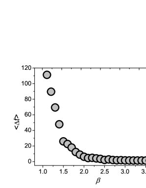
A serious problem in the above method is that for different $\beta$, the average inter-event times $\langle\Delta t\rangle$ are different, and thus it is not fair to compare systems with different $\beta$. In fact, when $\beta\leq 2$, the average inter-event time diverges for the infinite large systems. Figure 1 reports a simulation result for a finite system, from which it is obvious that when $\beta$ decreases from 2 to 1, the average inter-event time grows very fast. To eliminate the biased influence caused by different $\langle\Delta t\rangle$, we introduce a factor $m(\beta)$ to Eq. 5, as

$$\Delta t^{\prime}=m(\beta)\times(r\times(M^{1-\beta}-1)+1)^{\frac{1}{1-\beta}},$$ (7)

where $m(\beta)$ satisfies

$$\frac{\langle\Delta t\rangle_{\beta_{1}}}{\langle\Delta t\rangle_{\beta_{2}}}=\frac{m(\beta_{2})}{m(\beta_{1})}.$$ (8)

Without the loss of generality, we set $m(1)=1$ and thus

$$m(\beta)=\frac{\langle\Delta t\rangle_{1}}{\langle\Delta t\rangle_{\beta}}.$$ (9)

To summarize, in the initialization, given $M$ and $\beta$, $m(\beta)$ can be estimated directly by simulation, and then for each individual $i$, we first generate a random real $r$ in the range $[0,1]$ and then calculate her/his characteristic inter-event time $\Delta t_{i}$ according to Eq. 7.

Figure 3: Impacts of the power-law exponent $\beta$ on the epidemic spreading process. The first three plots show the number of infected nodes $I(t)$ versus the time step $t$, where the parameters are: (a) $N=1000$, $\lambda=3\times 10^{-4}$, (b) $N=2000$, $\lambda=3\times 10^{-4}$ and (c) $N=1000$, $\lambda=5\times 10^{-5}$. The plot (d) displays the first time step $t^{*}$ when the number of infected nodes exceeds half of the population. In plot (d), black squares, red circles and blue triangles correspond to the cases shown in plots (a), (b) and (c), respectively. All the data points are obtained by averaging over 10 independent runs.

Notice that, the generated inter-event time from Eq. 7 may be not well-pleasing for our model since it is generally not an integer. Here, for a real $\Delta t$, we firstly separate its integral and decimal parts as $\Delta t=\lfloor\Delta t\rfloor+b$, $b\in[0,1)$. Then we reset $\Delta t\leftarrow\lfloor\Delta t\rfloor$ with probability $1-b$, while $\Delta t\leftarrow\lfloor\Delta t\rfloor+1$ with probability $b$. For example, if we obtain $\Delta t=3.2$ from Eq. 7, it will be reset as 3 with probability 0.8 while 4 with probability 0.2. Figure 2 shows typical distributions for a system with $N=1000$ individuals for different $\beta$, from which one can see that the generating method for heterogeneous inter-event times well meets the requirement (The fitting exponents, shown as slopes in the figure, are obtained by using the maximum likelihood method [46]).

3 Results and Discussion

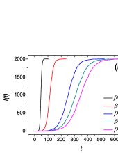
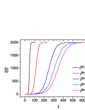
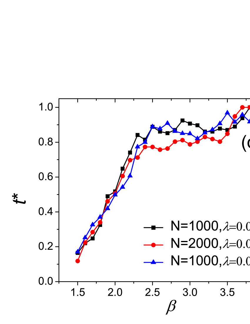
A set of comparative simulations are carried out to show the impacts of heterogeneous activity on spreading speed. Each run starts with one randomly selected node as infected node and the other $N-1$ nodes all susceptible. Figure 3 reports how the spreading speed, characterized by the number of infected nodes $I(t)$, is affected by the heterogeneity of the individual activities. Although each individual behaves in a perfectly uniform pace, the heterogeneity at the population level has remarkably impacts on the epidemic spreading, and the spreading can be accelerated by enhancing the heterogeneity (i.e., reducing the exponent $\beta$). To clearly show the relation between speed and heterogeneity, we further consider the required time steps $t^{*}$ to infect half population from the initialization. We normalize $t^{*}$ by dividing by $t^{*}_{\texttt{max}}$ given a parameter set $(N,\lambda)$, which is helpful in better displaying several $t^{*}(\beta)$ curves with different parameter sets $(N,\lambda)$. One can see from figure 3(d), $t^{*}$ monotonously increases with $\beta$, again indicating that the spreading can be accelerated by reducing $\beta$.

Figure 4: Impacts of the power-law exponent $\beta$ on the epidemic spreading process of the model for comparison. The first three plots show the number of infected nodes $I(t)$ versus the time step $t$, where the parameters are: (a) $N=1000$, $\lambda=3\times 10^{-4}$, (b) $N=2000$, $\lambda=3\times 10^{-4}$ and (c) $N=1000$, $\lambda=5\times 10^{-5}$. The plot (d) displays the first time step $t^{*}$ when the number of infected nodes exceeds half of the population. In plot (d), black squares, red circles and blue triangles correspond to the cases shown in plots (a), (b) and (c), respectively. All the data points are obtained by averaging over 100 independent runs.

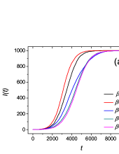
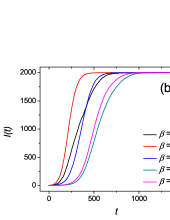
As we have mentioned before, the heavy-tailed distribution of inter-event time at the population level is well accepted, but whether the individual is heterogeneous is still under debate [34, 35]. With the assumption that each individual has heavy-tailed temporal activities, previous works have revealed the non-ignorable impacts on epidemic spreading [36, 37, 38], yet they have not answered the question whether the heterogeneity in population level will affect the spreading speed if each individual is homogeneous. Figure 3 clearly says “YES”!

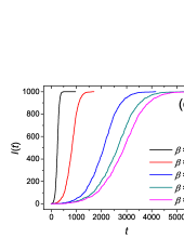
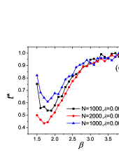
To make a comparison, we next investigate another model where each individual acts with a power-law inter-event time distribution $P(\Delta t)\sim\Delta t^{-\beta}$. Here $\beta$ is a system parameter, namely the inter-event time distributions of all individuals are the same. Of course, at the population level, the inter-event time distribution is also $P(\Delta t)\sim\Delta t^{-\beta}$. This model is closer to the assumption of previous works [36, 37]. As shown in Fig. 4, the exponent $\beta$ also affects the spreading process, but in a more complicated way [47]. In the range $\beta\in[1.5,4]$ and for $N=2000$, subject to $t^{*}$, the fastest spreading is about twofold faster than the slowest one in Fig. 4(d), while in Fig. 3(d), it can be tenfold faster. In a word, whatever the individual activities are homogeneous or not, the heterogeneity at the population level has remarkable impact on epidemic spreading. In comparison, a system consisted of heterogeneous individuals is more sensitive to the temporal heterogeneity of activities at the population level even though each individual acts in a completely periodical way. Qualitatively speaking, the difference between a system of regular agents with different acting rates and a system of non-Poissonian agents with the same statistics is analogous to the difference between quenched and annealed systems. In the former system, a few agents are born with very large $\Delta t$, which play the role of absorbing nodes that are hardly to infect other agents. In the latter system, each agent has the chance to suffer a very large $\Delta t$, but not usual. These two systems can be considered as a quenched system and an annealed system, respectively. We believe that the difference of impacts reported in this paper is similar to the difference of spreading processes in quenched and annealed networks [48, 49], however, to which extent the observed different impacts can be explained by the difference between quenched and annealed systems, as well as how to characterize and understand the difference between quenched and annealed systems are still open questions to us. To summarize, this work provides complementary information to the previous studies and refines our understanding of the impact of heterogeneous human activities on epidemic spreading.

References

- [1] R. M. Anderson, R. M. May, Infectious Diseases of Humans (Oxford University Press, 1991).
- [2] N. T. Bailey, The Mathematics of infectious diseases (Hafner Press, 1975).
- [3] H. W. Hethcote, SIAM Rev. 42, 599 (2000).
- [4] L. A. Meyers, B. Pourbohloul, M. E. J. Newman, D. M. Skowronski, R. C. Brunham, J. Theor. Biol. 242, 71 (2005).
- [5] Y. Yang, J. D. Sugimoto, M. E. Halloran, N. E. Basta, D. L. Chao, L. Matrajt, G. Potter, E. Kenah, I. M. Jr. Longini, Science 326, 729 (2009).
- [6] P. Wang, M. C. González, C. A. Hidalgo, A.-L. Barabási, Science 324, 1071 (2009).
- [7] A.-L. Barabási, IEEE Control Syst. Magazine 27(4), 33 (2007).
- [8] T. Zhou, X.-P. Han, B.-H. Wang, Towards the understanding of human dynamics, in M. Burguete, L. Lam (eds.) Science Matters: Humanities as Complex Systems (Singapore: World Scientific, 2008), arXiv: 0801.1289.
- [9] P. Gallagher, Math. Biosci. 63, 157 (1983).
- [10] D. J. Watts, S. H. Strogatz, Nature 393, 440 (1998).
- [11] A.-L. Barabási, R Albert Science 286, 509 (1999).
- [12] R. Pastor-Satorras, A. Vespignani, Handbook of Graph and Networks, eds. S. Bornholdt and H. G. Schuster (Wiley-VCH, Berlin, 2003).
- [13] T. Zhou, Z.-Q. Fu, B.-H. Wang, Prog. Nat. Sci. 16, 452 (2006).
- [14] A. Barrat, M. Weigt, Eur. Phys. J. B 13, 547 (2000).
- [15] R. Pastor-Satorras, A. Vespignani, Phys. Rev. Lett. 86, 3200 (2001).
- [16] D. Brockmann, L. Hufnagel, T. Geisel, Nature 439, 462 (2006).
- [17] M. C. Gonzálze, H. J. Herrmann, Physica A 340, 741 (2004).
- [18] M. C. Gonzálze, P. G. Lind, H. J. Herrmann, Phys. Rev. Lett. 96, 088702 (2006).
- [19] P. G. Lind, J. S. Jr Andrade, L. R. da Silva, H. J. Herrmann, Phys. Rev. E 76, 036117 (2007).
- [20] M. Tang, Z. Liu, B. Li, EPL 87, 18005 (2009).
- [21] S. Ni and W. Weng, Phys. Rev. E 79, 016111 (2009).
- [22] A.-L. Barabási, Nature 435, 207 (2005).
- [23] J. Candia, M. C. González, P. Wang, T. Schoenharl, G. Madey, A.-L. Barabási, J. Phys. A 41, 224015 (2008).
- [24] W. Hong, X.-P. Han, T. Zhou, B.-H. Wang, Chin. Phys. Lett. 26, 028902 (2009).
- [25] Y. Wu, C. Zhou, J.-H. Xiao, J. Kurths, H. J. Schellnhuber, Proc. Natl. Acad. Sci. U.S.A. 28, 068901 (2011).
- [26] Z.-D. Zhao, H. Xia, M.-S. Shang, T. Zhou, Chin. Phys. Lett. 28, 068901 (2011).
- [27] Z. Dezsö, E. Almaas, A. Lukács, B. Rácz, I. Szakadát, A.-L. Barabási, Phys. Rev. E 73, 066132 (2006).
- [28] B. Gonçalves, J. J. Ramasco, Phys. Rev. E 78, 026123 (2008).
- [29] F. Radicchi, Phys. Rev. E 80, 026118 (2009).
- [30] J. Leskovec, J. Kleinberg, C. Faloutsos, in Proceedings of the SIAM International Conference on Data Mining, 2007.
- [31] T. Zhou, H. A. T. Kiet, B. J. Kim, B.-H. Wang, P. Holme, EPL 82, 28002 (2008).
- [32] Z.-D. Zhao, T. Zhou (unpublished).
- [33] A. Vázquez, J. G. Oliveira, Z. Dezsö, K.-I. Goh, I. Kondor, A.-L.Barabási, Phys. Rev. E 73, 036127 (2006).
- [34] C. A. Hidalgo, Physica A 369, 877 (2006).
- [35] R. D. Malmgren, D. B. Stouffer, A. E. Motter, L. A. N. Amaral, Proc. Natl. Acad. Sci. U.S.A. 105, 18153 (2008).
- [36] J. L. Iribarren, E. Moro, Phys. Rev. Lett. 103, 038702 (2009).
- [37] A. Vázquez, B. Rácz, A. Lukács, A.-L. Barabási, Phys. Rev. Lett. 98, 158702 (2007).
- [38] M. Karsai, M. Kivela, R. K. Pan, K. Kaski, J. Kertész, A.-L. Barabási, J. Saramaki, arXiv: 1006.2125.
- [39] M. Barthélemy, A. Barrat, R. Pastor-Satorras, A. Vespignani, Phys. Rev. Lett. 92, 178701 (2004).
- [40] T. Zhou, G. Yan, B.-H. Wang, Phys. Rev. E 71, 046141 (2005).
- [41] G. Yan, T. Zhou, J. Wang, Z.-Q. Fu, B.-H. Wang, Chin. Phys. Lett. 22, 510 (2005).
- [42] A. Vázquez, Phys. Rev. Lett. 96, 038702 (2006).
- [43] T. Zhou, J.-G. Liu, W.-J. Bai, G. Chen, B.-H. Wang, Phys. Rev. E 74, 056109 (2006).
- [44] W.-J. Bai, T. Zhou, B.-H. Wang, Physica A 384, 656 (2007).
- [45] A. Clauset, C. R. Shalizi, M. E. J. Newman, SIAM Rev. 51, 661 (2009).
- [46] M. L. Goldstein, S. A. Morris, G. G. Yen, Eur. Phys. J. B 41, 255 (2004).
- [47] It is very interesting that the effetc of is not “monotonous”. As shown in Fig. 4(a)-4(c), the process with is the fastest, and more clearly can be found in Fig. 4(d), has an “optimal” value subject to the fastest spreading at about 1.8. This complicated phenomenon has not been observed in the previous models and we will discuss it (with analytical solution on ) in another paper.
- [48] P. L. Doussal, J. Machta, Phys. Rev. B 40, 9427(R) (1989).
- [49] A. Baronchelli, R. Pastor-Satorras, Phys. Rev. E 82, 011111 (2010).